Assessing Light Non-Aqueous Phase Liquids in the Subsurface Using the Soil Gas Rn Deficit Technique: A Literature Overview of Field Studies

Abstract

²²²Radon (Rn) was proposed in the late 1990s as a naturally occurring tracer for light non-aqueous phase liquids (LNAPLs) in the subsurface, due to its preferential partitioning behavior in the non-aqueous phase, resulting in a reduction in Rn activities in areas with LNAPLs in the subsurface compared to unimpacted areas (Rn deficit). The Rn deficit technique emerged as a cost-effective, non-invasive, and sustainable method to rapidly identify and quantify LNAPLs, for the characterization and monitoring of contaminated sites. This paper presents an overview of the technique and its field applications, with a specific focus on the use of the method in the vadose zone based on soil gas Rn measurements. Although various configurations have shown favorable outcomes, limitations persist in the application of the soil gas Rn deficit technique. Deep LNAPL contamination, soil matrix heterogeneity, and temporal variations in Rn emissions pose challenges to quantitative evaluations of LNAPL contamination. Recognizing these factors is crucial for site-specific assessments. This review aims to highlight both the strengths and limitations of the method, providing insights into potential areas for future research while acknowledging the positive outcomes achieved in different configurations over the past decades.

1. Introduction

The hydrocarbon contamination of soil and groundwater, with the presence of light non-aqueous phase liquids (LNAPLs), is a major, global, environmental concern [1,2]. LNAPL results mainly from spills of fuels and oils, and its wide range of constituents represents some of the most commonly encountered organic contaminants in the subsurface environment [3]. The characterization of petroleum-contaminated sites has evolved over time, improving the efficiency of the interventions in terms of time and cost [4]. However, it is worth noting that the assessment of LNAPL occurrence and distribution at these sites typically involves the use of traditional methods, including the collection of soil cores to be analyzed in specialized laboratories and the installation of groundwater monitoring wells to measure the apparent thickness of the potentially present supernatant [5]. However, these methods may not always provide enough information for a complete site assessment and effective remediation planning and monitoring [6,7]. In order to address the challenges posed by both these technological and economic barriers, different techniques have been implemented and tested in real field conditions during the last decades [3,6,7,8,9,10,11,12,13,14,15,16]. A concise summary of these methods is provided in Section 2. The use of tracers to characterize and monitor LNAPL and to evaluate the effectiveness of in situ remediation has been investigated as one of the potential alternative approaches [17]. The potential use of ²²²Radon (Rn), as a natural tracer characterized by a preferential partitioning into LNAPL, has been studied in this regard, as a sustainable alternative, since the late 1990s, e.g., [18,19,20,21,22,23,24,25,26,27,28,29,30].

In 2015, Schubert [22] published a comprehensive review on the suitability of Rn as an NAPL tracer, providing background theoretical information on Rn partitioning behavior and discussing three potential applications of the technique, including NAPL investigations in soils and aquifers and groundwater remediation monitoring. This study provides an update of this review, with a specific focus on the use of the subsurface Rn deficit technique for the assessment of LNAPL contamination in the vadose zone, which was further studied and tested in the last decade. The theoretical background on the potential of soil gas Rn as an environmental indicator of LNAPL contamination is briefly summarized in Section 3. The paper then provides insight into the analytical description of subsurface soil gas Rn activity concentrations, the resulting deficit in the case of LNAPL contamination, and the prediction of LNAPL saturations, considering both subsurface equilibrium conditions and gas transport (Section 4). An overview of the practical application of the method tested over the past two decades, with a focus on field applications involving soil gas Rn measurements, is later discussed (Section 5), with particular emphasis on the different approaches used for sampling and analysis. The review summarizes the findings of the examined papers and the potential of the method, considering the positive results and the limitations that have emerged and that still need to be addressed in future research and experimentation (Section 6).

2. LNAPL Detection

There are two main drivers in the need for site characterization and LNAPL management: understanding the potential risks posed to receptors by current and possible future mobile LNAPL distributions, and comprehending LNAPL constraints on remediation selection, design, and operation [3]. Site characterization is both an initial assessment process and an ongoing process that may remain essential throughout the remediation program for a site. For large and complex sites, it may be advantageous to use an approach that incorporates multiple lines of evidence and various integrated multi-disciplinary techniques to gather high-quality data that can serve as a foundation for the development of management plans [31]. On smaller and less complex projects, the amount of investigation may be scaled down. For the identification of the presence of LNAPL, the determination of the state in which it is found, the extent of the contamination, and the monitoring in terms of spatial evolution and concentration, there are several possible approaches. Table 1 summarizes some of the tools available and highlights the information that can be obtained from their respective uses.

Soil characterization by soil sampling is one of the primary methods used to assess soil contamination and the relative contaminant concentrations. Soil sampling systems were originally developed to sample unconsolidated material from a given depth to characterize lithology and mineralogical composition. Soil contamination characterization typically involves the collection of soil samples at various depths and the laboratory analysis of the samples to determine chemical concentrations and composition, providing a direct quantitative estimate of the contamination [3]. The main advantages of soil characterization by soil sampling relate to its ability to provide a quantitative estimate of contamination and its composition. On the other hand, cost is its main disadvantage because of the expenses associated with drilling, sampling, and quantitative analysis [32]. Groundwater monitoring wells are typically installed at sites contaminated or suspected of being contaminated with petroleum products and are commonly used to monitor the possible presence of free LNAPL as supernatant on top of the water level in the well. However, this method alone is inadequate for quantifying LNAPL saturations or identifying LNAPL in all groundwater and contamination conditions. In fact, the absence of LNAPL in a monitoring well does not necessarily indicate the absence of LNAPL in the soil. The product may be present in concentrations that prevent it from moving freely in the subsurface (residual LNAPL), and, therefore, it may not enter the well screen as a supernatant product. Moreover, if present, the measurable in-well LNAPL thickness (apparent thickness) may differ from the actual thickness of the product in the aquifer [33]. Furthermore, groundwater table fluctuations due to seasonal variations or artificial pumping can bring a redistribution of LNAPL to the affected area of the subsurface (smear zone), affecting the occurrence of LNAPL in both the aquifer and wells [34,35]. In addition to traditional sampling methods, in situ penetration tests have become a popular approach for site investigation [32]. Direct push investigation tools can be coupled with sensors to provide information on subsoil contamination. Specifically, for LNAPL, probes such as the Membrane Interface Probe (MIP), the Laser-induced fluorescence (LIF), and the Optical Image Profiler (OIP) [3,15] are often used. Although promising, these methods are considered to provide screening-level data that need to be supplemented with analytical information and should not be used as a replacement for traditional soil sampling and monitoring wells. Instead, they should be used as an instrument to optimize the number of borings and monitoring wells needed to meet site characterization targets [7]. The use of nonintrusive methods is also considered a valuable alternative, as is the case of geophysical techniques such as electrical resistivity tomography (ERT), ground-penetrating radar (GPR), and induced polarization (IP) [7,8,9,16,36]. Surface geophysical methods are suitable for both large-scale investigations and small-scale site characterization and can be used to map subsurface properties that affect contaminant transport and, under specific conditions, to identify contamination indicators [7]. However, they are not suitable for the direct measurement of concentrations of specific contaminants. The interpretation of data obtained from geophysical methods can often be challenging and lead to unclear results, but the combination of different techniques can resolve potential ambiguities that may arise from the measurement of a single geophysical parameter [37]. It should also be noted that geophysical approaches such as ERT and IP require the installation of electrodes on the ground surface and good ground contact. The inability to drill on the concrete surface of some contaminated sites limits the use of these geophysical methods [7].

Direct soil gas monitoring in the vadose zone is also used as a screening tool for locating potential contamination sources and planning the localization of monitoring wells [6,38]. The results can be considered a qualitative indicator of LNAPL impacts for volatile and semi-volatile hydrocarbons. Soil gas investigation can also be used to investigate natural source zone depletion (NSZD) rates and hydrocarbon degradation [39]. It is important to note that soil gas analysis is considered qualitative or semi-quantitative and generally cannot quantify LNAPL in the source zone, but has been successfully used as a screening technique at many contamination sites and often led to a more focused and cost-effective investigation of source areas [3]. However, these methods can provide misleading results if subsurface contamination conditions are not adequately understood, as the results can be affected by various factors, such as complex vapor transport pathways, and have limitations when dealing with sites containing non-volatile LNAPL [6]. Different tracer-based methods have been developed and tested to determine their ability to estimate the location, amount, and distribution of NAPL contamination in laboratory and field conditions [3]. Various types of tracers have been studied in this context, including interfacial tracers that concentrate at the interface between NAPL and water, biogeochemical tracers used to estimate abiotic and biotic reactions, and partitioning tracers’ selective partitioning behavior into the NAPL [17]. In the latter approach, the partitioning tracers, such as alcohols (e.g., isopropanol and 2,2-dimethyl-3-pentanol), are injected in groundwater together with non-reactive tracers and their retardation factors are determined by measuring their concentrations in one or more control wells [17,40,41]. The migration of these tracers is then monitored at extraction wells. These data, together with specific partitioning characteristics of each tracer, dependent on the aquifer material and NAPL [42], can be used to locate and quantify NAPL contamination [20]. These methods were primarily tested for dense NAPLs (DNAPLs), which are typically found in the deeper zones of the aquifer. It should be noted that this approach involves injecting chemicals as tracers, which can be costly and raise additional environmental concerns [32]. A recently studied, viable alternative is the use of the subsurface naturally occurring ²²²Rn as a partitioning tracer for NAPL detection [15]. The following section provides some additional information on ²²²Rn, with a specific focus on its behavior as a gas in the subsurface.

Table 1. Comparison of the information provided by different LNAPL characterization tools. The solid symbol indicates that the method is capable of providing the information reported in the column. The empty symbol indicates that the method is potentially applicable or that can only provide semi-quantitative information.

Technique	Information Provided
	Mobile LNAPL Presence	Residual LNAPL Presence	LNAPL Saturation	LNAPL Composition	TPH Concentrations in Soil	TPH Concentrations in Water
Soil sampling	○	●	○	○	●
Groundwater sampling (monitoring wells)	●			●		●
Direct push analytical technologies (MIP, LIF, OIP)	●	●	○		○	○
Surface geophysical methods (ERT, IP, GPR)	●	●
Soil gas sampling	○	○			○	○
Tracer techniques	●	●	○			○
Radon	●	●	○		○	○

● The method is capable of providing the information reported in the column; ○ the method is potentially applicable or can only provide semi-quantitative information.

Table 1. Comparison of the information provided by different LNAPL characterization tools. The solid symbol indicates that the method is capable of providing the information reported in the column. The empty symbol indicates that the method is potentially applicable or that can only provide semi-quantitative information.

Technique	Information Provided
	Mobile LNAPL Presence	Residual LNAPL Presence	LNAPL Saturation	LNAPL Composition	TPH Concentrations in Soil	TPH Concentrations in Water
Soil sampling	○	●	○	○	●
Groundwater sampling (monitoring wells)	●			●		●
Direct push analytical technologies (MIP, LIF, OIP)	●	●	○		○	○
Surface geophysical methods (ERT, IP, GPR)	●	●
Soil gas sampling	○	○			○	○
Tracer techniques	●	●	○			○
Radon	●	●	○		○	○

● The method is capable of providing the information reported in the column; ○ the method is potentially applicable or can only provide semi-quantitative information.

3. Radon

Radon is a chemically inert, colorless, and odorless noble gas. It is the heaviest known gas, with a density of 9.72 g L⁻¹ at 0 °C (i.e., 8 times higher than that of air). It is naturally present in the earth’s crust and it is a radiogenic gas, produced by the radioactive decay process of ²²⁶Ra, and is itself naturally radioactive, decaying directly into ²¹⁸Po [43]. Radioactive decay is the phenomenon of emission of energy in the form of ionizing radiation, like alpha particles, beta particles, and/or gamma rays. It occurs in unbalanced atoms called radionuclides, which decay into different atoms, known as decay products. This process continues until a stable state is reached, at which point the atom is no longer radioactive. The radionuclides that undergo multiple decays are known as series radionuclides, and the sequence of decay products they produce is called the decay chain. All decay products within the chain are radioactive, except for the final stable atom. Each radionuclide has a specific decay rate, measured in terms of its half-life, the time required for half of the radioactive atoms present to decay [44].

Several isotopes of radon exist, depending on the referred decay chain. The naturally occurring isotopes that are found in greater quantities are [45]:

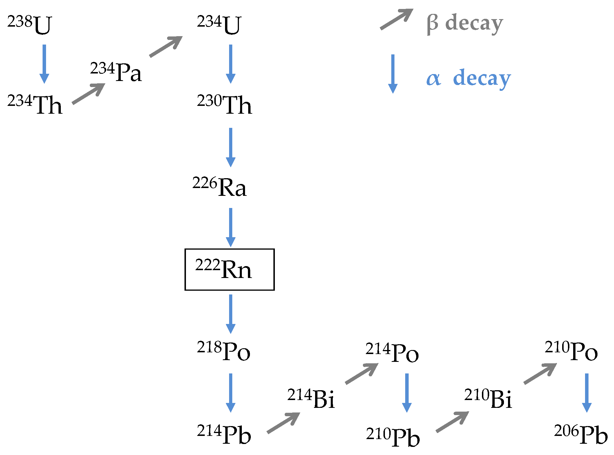
• ²¹⁹Rn, actinon, which belongs to the radioactive series of ²³⁵U, is formed by the decay of ²²³Ra and decays in ²¹⁵Po. It is characterized by a half-life of 3.92 s and is naturally present in very low amounts;
• ²²⁰Rn, thoron, which belongs to the radioactive series of ²³²Th, is formed by the decay of ²²⁴Ra and decays in ²¹⁶Po. Thoron has a half-life of 55.6 s, but the isotope that produces it is instead quite abundant in nature;
• ²²²Rn, radon, a more stable isotope, which belongs to the radioactive series of ²³⁸U, is formed by the decay of ²²⁶Ra and decays in ²¹⁸Po (Figure 1). It has the highest half-life of all isotopes, at 3.825 days, and is present in almost all mineral grains in the soils and rocks of the earth’s crust.

This paper discusses the behavior of the latter isotope, hereafter referred to as radon (Rn), which is the most studied and of interest in several fields due to its higher half-life and abundance in nature compared to the others.

Rn is considered a health hazard since exposure to the gas over a long period increases the risk of developing lung cancer [46]. Soil and rock are the primary sources of Rn exposure for people. The only other relevant sources are building materials [47]. During air inhalation, both Rn and its decay products can be inhaled. While Rn is normally expelled on exhalation due to its chemical properties, some of the decay products may remain in the respiratory system. These decay products emit alpha particles, which can affect the lung tissue and potentially cause the formation of cancer cells. Also, the presence of dissolved Rn in drinking water can cause an increased risk of cancer. However, the majority of the risk associated with Rn in water is due to inhalation of the fraction released into the air, rather than ingestion of the water itself [48].

In addition to its association with human health risks, Rn is also studied for its potential applications in the environmental field. Researchers are studying its behavior in the soil as a potential seismic precursor, and it is used in hydrological research to assess interactions between deep and surface waters due to its rapid dispersion in the air [49]. Additionally, it is being studied as an environmental tracer due to its ubiquitous presence in nature, detectability, and inert behavior. Since radium is present in almost all minerals, Rn is constantly produced in every soil or aquifer matrix [22]. As an environmental tracer, it has the advantage of not creating additional environmental contamination, not altering the physical and chemical balance of the studied medium, and being suitable for large-scale and long-term studies [50]. An overview of Rn applications as an environmental tracer in hydrogeological and geological investigations is provided by Sukanya et al. [51]. One of the applications briefly discussed is the use of Rn as an environmental tracer for the assessment of NAPL contamination [22] in both the saturated [18,24,28,30,52,53,54] and vadose zone [19,21,23,26,29,55,56,57,58,59,60], due to its tendency to preferentially partition into organic phases. To implement and use Rn as a tracer for environmental applications, it is crucial to comprehend the mechanisms of its production and behavior in the subsurface. The following section briefly summarizes these mechanisms.

3.1. Radon Migration Process in the Subsurface and Its Influence Factors

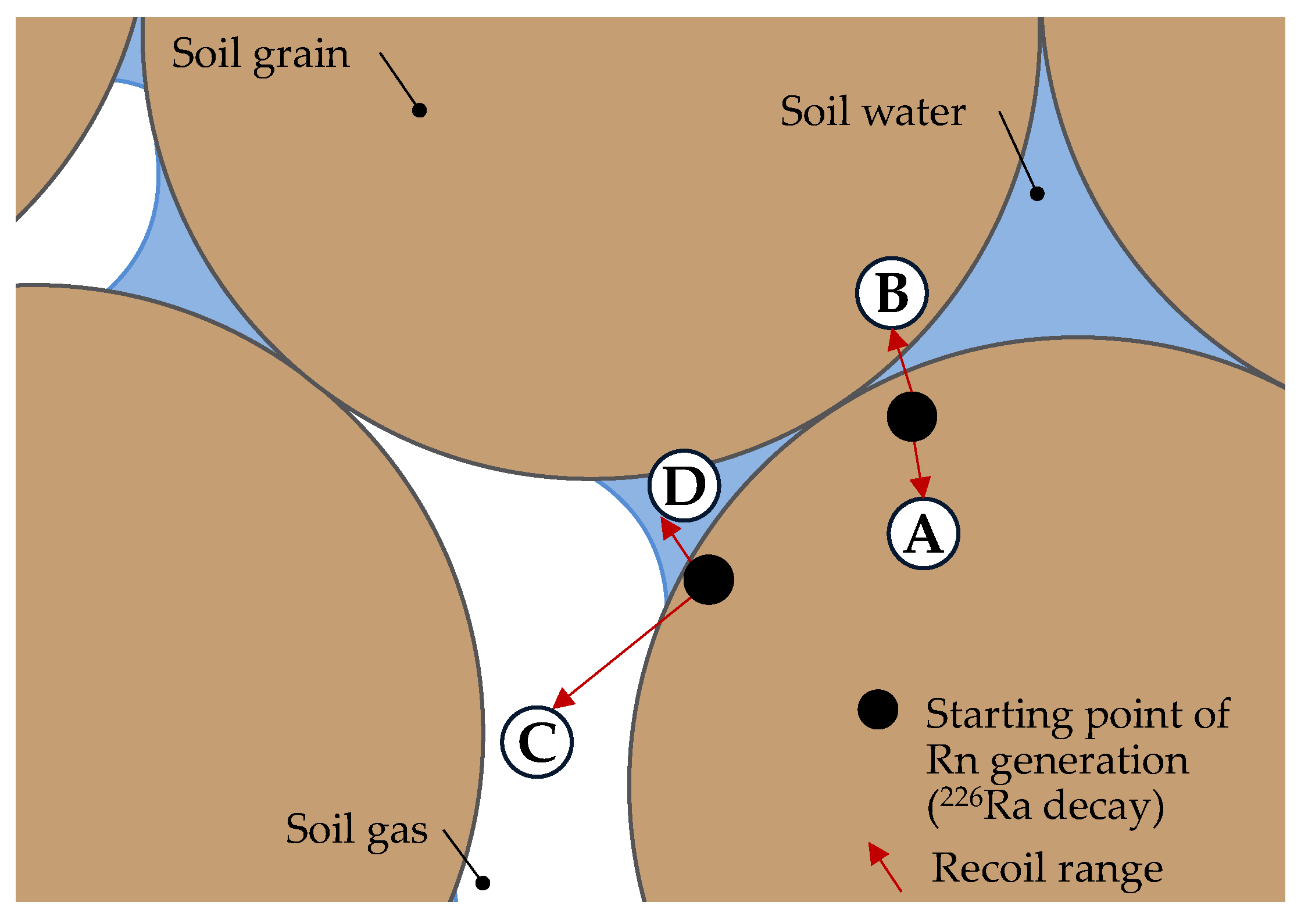
The geological characteristics of a site, such as lithology, porosity, and fluid contents, affect the Rn activity concentrations detectable in the subsoil. The activity of a radioactive sample containing a radionuclide at a determined energetic level is the number of spontaneous disintegrations produced in a unit of time, indicating how fast the substance disintegrates with time [45]. The activity of a radioactive element is measured in units of Becquerels (Bq), which represents the number of atoms required to create one radioactive decay per second. The activity concentration of a radionuclide can be defined in terms of volume, expressed in Bq m⁻³, or mass, expressed in Bq kg⁻¹.

The activity concentration of soil and rock ²²⁶Ra corresponds to a production rate of ²²²Rn per unit mass of the material. The activity concentration A of a radionuclide is determined by the number of atoms N and its radioactive decay constant λ, where A = N·λ [61]. Thus, a ²²⁶Ra content of 1 Bq kg⁻¹ corresponds to a production rate of 1 atom kg⁻¹ s⁻¹ for ²²²Rn, which is equivalent to 2.1 × 10⁻⁶ Bq kg⁻¹ s⁻¹ (using the radioactive decay constant λ for ²²²Rn of 2.1 × 10⁻⁶ s⁻¹). The content of radium and uranium, Rn precursors, varies among different types of rocks (

Table 2. Typical uranium activity concentrations in certain rock types [62].

Rock Type	238U (Bq kg−1)
Igneous—Acidic (e.g., granite)	59.2
Igneous—Intermediate (e.g., diorite)	22.9
Igneous—Mafic (e.g., basalt)	11.5
Igneous—Ultrabasic	0.4
Sedimentary—Limestone	27.7
Sedimentary—Carbonate	26.6
Sedimentary—Sandstones	18.5
Sedimentary—Shale	44.4

). For instance, acid igneous rocks such as granites, some types of bituminous shale, and phosphatic rocks typically exhibit higher average uranium concentrations.

Being an inert gas with no tendency to form chemical bonds, Rn can move through porous materials such as soil even at significant distances from the point of generation. It can migrate in the subsurface by diffusion through the pores in the opposite direction to the concentration gradient, pressure-induced advection, and convective transport by another fluid. As an example, several studies have reported high radon activities in soil gas due to advective transport facilitated by carrier gases through faults and fractured areas, characterized by high permeability, which may be further increased by seismic activity [63,64]. Rn can then be released from the soil surface into the atmosphere or enter buildings through cracks, porous building materials, and other pathways [47] if decay has not yet occurred. The different processes mentioned here, from generation to exhalation from the surface, are detailed below.

3.1.1. Emanation

When a ²²⁶Ra atom decays into a Rn atom, it generates alpha particles that move in the opposite direction of the Rn atom, which continues to move in its direction until it transfers its energy to another material. This distance, called recoil range, is typically 20–70 nm in common solid materials, 100 nm in water, and 63 μm in air [65]. Depending on the point of Rn generation in the soil material, and the geometry of the grains, therefore, three situations can occur: after having traveled a short distance, the atom remains inside the same grain of soil (case A of Figure 2); the atom passes through a pore and enters an adjacent grain (case B of Figure 2); the atom is ejected from the grain, arriving in the interstitial space, and is later expelled by soil gases (case C of Figure 2) or water (case D of Figure 2) [66]. The release of Rn into soil pores is primarily caused by the phenomenon of recoil. Emanation by diffusion can be disregarded due to the extremely low Rn diffusion coefficient in mineral matrices, which ranges from 10⁻³¹ to 10⁻⁶⁹ m² s⁻¹, resulting in diffusion lengths between 10⁻⁷ and 10⁻²⁶ μm [61].

The emanation coefficient is a crucial parameter that characterizes the physical behavior of Rn in the context of emanation. It represents the fraction of Rn atoms that escape from mineral grains into the interstitial space. Various methods exist to determine its value, all based on measuring the maximum Rn concentration emanating from a sample in a closed space after achieving secular equilibrium, along with measuring radium in the same sample [61].

Several factors can affect the emanation coefficient value. For instance, the distribution of ²²⁶Ra is not homogeneous throughout the volume of the soil grain but rather is concentrated on its surface [68]. Because smaller grains have a higher surface area-to-volume ratio, this results in larger amounts of radium and higher values of the emanation coefficient for finer-grained soils. Furthermore, with smaller grains, Rn is more easily carried out of the grain itself in the recoil phenomenon [61]. Additionally, as the water content increases, there is an increase in emission due to the smaller recoil range of Rn in water compared to air. This reduces the fraction of Rn atoms that enter an adjacent grain by recoil and increases the fraction of atoms that remain in the water and thus in the interstitial space [66]. It was also shown that, with a high water content in the soil, close to saturation conditions, the emission coefficient remains almost constant [47]. It was observed that the emanation coefficient reaches a maximum value for water content of 5% for general soil type, 1–2% for gravel, and 10–15% for clay [69].

It must be considered that there is a direct relationship between the Rn emanation coefficient in the soil and temperature. An increase in temperature causes a decrease in the physical adsorption of Rn onto grains. Consequently, the Rn diffusion coefficient increases, and its concentration in pore air increases as well [25,70]. The emanation coefficient at different temperatures can be estimated using the following equation [71]:

$$\mathsf{\epsilon }={\mathsf{\epsilon }}_{\mathrm{m}}+0.0021·(\mathrm{T}-{\mathrm{T}}_{\mathrm{m}})$$

(1)

where ε (-) is the calculated emanation coefficient at the temperature T (°C), ε_m (-) is the measured or known emanation coefficient, and T_m (°C) is the soil temperature at the time of sampling.

3.1.2. Partitioning in Soil Pores

In the case of uncontaminated soil, the distribution of Rn atoms in the soil can be classified into four states: incorporated into solid soil grains, sorbed to the surface of soil particles, dissolved in the pore water, and dispersed in the pore gas phase. As discussed in the previous section, the diffusion of Rn inside the soil grain is extremely slow and can be neglected. The exchange of Rn atoms among the remaining three states may be rapid relative to the half-life of Rn [61]. Rn displays moderate solubility in water, with a value of 230 cm³ kg⁻¹ at 20 °C and 1 atm [72]. As a result, it can dissolve in subsoil pore water and be transported by groundwater in the saturated zone. However, Rn absorption in water is reversible, and its tendency to be desorbed, considering the value of the water/air partition coefficient, is quite high. At a temperature of 20 °C, the dimensionless partition coefficient of Rn between water and air k_w/g is in fact approximately 0.25. Therefore, the equilibrium Rn concentration in air is about four times that of Rn in water [19]. The dimensionless Henry’s constant for Rn, H (-), which is the inverse of k_w/g, is a function of temperature T, following the relationship [61,73]

$$\mathrm{H}\left(\mathrm{T}\right)=\frac{1}{(0.105+0.403·{\mathrm{e}}^{-0.0502·\mathrm{T}})}$$

(2)

where T is expressed in °C. Note that the empirical relationship is consistent with experimental results, resulting in the coefficient values reported in

Table 3. Dimensionless Henry’s constant values for Rn [74].

Temperature °C	Dimensionless Henry’s Constant (H)
0	1.875 ± 0.155
10	2.365 ± 0.255
20	3.65 ± 0.27
30	5.27 ± 0.34

[74].

The interaction of Rn with the surface of soil grains can be a relevant factor in emanation and transport processes in dry soil conditions [61]. The partitioning of Rn between the gas and sorbed phases can be described by a linear sorption isotherm, and by the partition coefficient between the sorbed phase and gas phase k_s/g (k_s/g of 1.4 × 10⁻⁵ m³ kg⁻¹ [75], for example, for a sandy clay loam). However, for typical environmental soil moisture levels, sorption effects are expected to be smaller and are often neglected [61].

3.1.3. Transport

On long-term averages, existing information indicates that Rn transport from the soil to the atmosphere occurs primarily via diffusion [61]. Due to the higher Rn concentrations in soil gas compared to the atmosphere, Rn atoms diffuse through interstitial pores and migrate toward the soil surface. Fick’s law describes the diffusive flux J_diff (Bq m⁻² s⁻¹), directly proportional to the concentration gradient ∇Rn:

$${\mathrm{J}}_{\mathrm{d}\mathrm{i}\mathrm{f}\mathrm{f}}=-{\mathrm{D}}_{\mathrm{e}}·\nabla \mathrm{R}\mathrm{n}$$

(3)

where Rn (Bq m⁻³) is the Rn activity concentration and D_e (m² s⁻¹) is the Rn effective diffusion coefficient. The effective diffusion coefficient in the subsoil generally varies with the properties of the species being diffused, the pore structure, the types of fluids present in the pores, the degree of fluid saturation, the temperature, and the adsorption properties of the solid matrix. Various models can be utilized to estimate its value, depending on these parameters, as those of Penman [76,77], Marshall [78], Millington and Quirk [79], and Millington and Shearer [80]. The soil’s water content significantly affects the effective diffusion coefficient of Rn in an inversely proportional manner since the Rn diffusion coefficient in water is about four orders of magnitude lower than that in air. Both values are shown below in

Table 4. Rn diffusion coefficients in air and water at 20 °C.

Parameter	Value	Reference
Rn diffusion coefficient in air Dmg	1.2 × 10−5 m2 s−1	[82]
Rn diffusion coefficient in water Dmw	1.16 × 10−9 m2 s−1	[83]

. Note that when the soil is drier, Rn’s ability to migrate into the soil increases even though the rate of emanation decreases. Instead, when the water content increases, the rate of emanation also increases but the diffusivity and permeability of the soil are significantly reduced [81].

It is also observed that the Rn diffusion coefficient decreases as the soil and sand grain size decrease, due to the decrease in porosity and increase in the bulk density [84].

It is important to note that advective transport can occur in the subsurface under the influence of pressure gradients, in addition to diffusive transport, which is typically considered predominant [85,86]. Darcy’s Law can be used to describe the advective transport of fluids in porous media when the flow is laminar and viscosity dominates the resistance to flow. From Darcy’s Law differential form, Rn advective flow J_adv (Bq m⁻² s⁻¹) can be expressed as

$${\mathrm{J}}_{\mathrm{a}\mathrm{d}\mathrm{v}}=-\mathrm{R}\mathrm{n}·\frac{{\mathrm{k}}_{\mathrm{g}}}{\mathsf{\mu }}·\nabla \mathrm{p}$$

(4)

where Rn (Bq m⁻³) represents the Rn activity concentration, k_g (m²) is the gas permeability of the soil, μ (kg m⁻¹ s⁻¹) is the dynamic viscosity of the fluid, and ∇p (kg m⁻² s⁻²) is the pressure gradient. Advection may be significant, particularly in the surface layer (approximately the first meter) of the soil due to barometric pressure gradients [87,88]. At greater depths, advection is typically caused by the presence of faults and fractures with the presence of gas carriers, such as CO₂ and CH₄ [89,90]. Local advection can also occur in conditions such as significant fluctuations of the groundwater table level [91,92,93] and can be enhanced in soil materials with high permeability and fractures that create preferential pathways in the soil gas [86,94].

3.1.4. Exhalation

Soil gas Rn is transported through the soil toward the surface and released into the atmosphere in a process known as exhalation. The exhalation rate is the number of Rn atoms released from a surface unit into the atmosphere that can be expressed per unit time (Bq m⁻² s⁻¹) or as a mass exhalation rate (Bq kg⁻¹ s⁻¹). Rn’s exhalation rate J_exh (Bq m⁻² s⁻¹) can be calculated as [67]

$${\mathrm{J}}_{\mathrm{e}\mathrm{x}\mathrm{h}}={\mathsf{\rho }}_{\mathrm{s}}·\mathsf{\epsilon }{·\mathrm{C}}_{\mathrm{R}\mathrm{a}}{·\left(\mathsf{\lambda }·{\mathrm{D}}_{\mathrm{e}}\right)}^{\frac{1}{2}}$$

(5)

where ρ_s (kg m⁻³) is the soil density, ε (-) is the Rn emanation coefficient, C_Ra (Bq kg⁻¹) is the radium activity concentration in the soil, λ (s⁻¹) is the Rn decay constant, and D_e (m² s⁻¹) is the Rn effective diffusion coefficient.

The process of exhalation is influenced by various factors. Some of these, such as soil water content, porosity, grain size, and temperature, have an influence on the Rn emanation and diffusion coefficient and, therefore, indirectly affect the exhalation rate [67]. On the other hand, other factors, such as the pressure difference between the ground surface and the soil, have a more direct impact on the exhalation phenomenon. A negative pressure difference occurs when the pressure at the ground surface is lower than the deep soil pressure. This results in an increase in Rn exhalations, as soil gas is transported towards the surface from deeper layers, where Rn concentration is higher. Conversely, a positive pressure difference occurs oppositely, causing a downward advective motion of gas. Other external parameters that influence the exhalation rate include wind (which is directly proportional) and rainfall (which is inversely proportional in the case of heavy rainfall) [67,90]. Daily variations in the Rn flux are mainly attributed to soil temperature. It was observed that the Rn flux is highest in the afternoon when temperatures are at their highest and soil water content is at its lowest [90,95]. High exhalation rates are typically found in seasons characterized by lower precipitation and low water content [96,97,98,99].

4. Radon as a Natural Tracer for the Identification of LNAPL Contamination

As described in the previous section, Rn activity concentration in the subsoil tends to reach equilibrium conditions as a result of constant emission and decay mechanisms [61]. This equilibrium is governed by the soil matrix and can be perturbed by the existence of LNAPL in the soil pores [18]. In fact, Rn in soil pores tends to be partitioned into the LNAPL, leading to a decrease in Rn activity in both aqueous and gaseous interstitial phases (Figure 3). Studies [18,20,21,22,23,24,25] have shown that in areas of the subsurface contaminated with LNAPLs, a local reduction in Rn activity concentration in groundwater or soil gas occurs, compared to unaffected areas. This decrease is known as the Rn deficit. Thus, the Rn deficit technique [18] has been studied to assess the existence of LNAPL in the subsurface. With this approach, the mean Rn activity concentration in an unpolluted area can be assumed as the background value of the site. Note that the background value is a function of soil properties such as the radium content (from which Rn derives), the dimensionless Rn emanation coefficient, soil porosity, and soil density [100]. In the presence of LNAPL, Rn partitions between soil pores containing water, gas, and LNAPL phases [19]. Assuming linear partitioning, it is theoretically possible to estimate the activity of Rn in soil gas or groundwater in the presence of a known amount of LNAPL. Reciprocally, under real conditions, it is possible to derive the amount of LNAPL from the Rn activities determined in the field. Concerning soil gas, different approaches can be used to describe the relationship between the predicted or measured Rn deficit in soil gas and the subsurface LNAPL saturation in the investigated area. Two approaches, which have been used for both theoretical studies and practical applications, are described below. The first approach considers equilibrium conditions in the subsurface and does not account for the variation of soil gas Rn activity concentration in the vertical soil profile, while the second approach instead includes the transport of Rn in soil gas.

4.1. Radon Deficit in the Subsurface in Equilibrium Conditions

Under the assumption of equilibrium conditions, Rn activity concentration in the soil pores, in an uncontaminated (background) area Rn₀ (Bq m⁻³), can be described as [100]

$$\mathrm{R}{\mathrm{n}}_0=\frac{\mathsf{\epsilon }{·\mathrm{C}}_{\mathrm{R}\mathrm{a}}·{\mathsf{\rho }}_{\mathrm{s}}}{{\mathsf{\theta }}_{\mathrm{t}}}$$

(6)

where ε (-) is the Rn emanation coefficient, C_Ra is the ²²⁶Ra concentration of the solids (Bq kg⁻¹), ρ_s is the dry soil bulk density (kg m⁻³), and θ_t is the soil porosity (-). Given the coexistence of water and gas in soil pores, the following relationship can be written [18]:

$$\mathrm{R}{\mathrm{n}}_0=\mathrm{R}{\mathrm{n}}_{\mathrm{w},\mathrm{b}}{·\mathrm{S}}_{\mathrm{w},\mathrm{b}}+\mathrm{R}{\mathrm{n}}_{\mathrm{b}}·{\mathrm{S}}_{\mathrm{g},\mathrm{b}}$$

(7)

where Rn_w,b (Bq m⁻³) and Rn_b (Bq m⁻³) are, respectively, the Rn activity concentration in equilibrium conditions in the water and gas, and S_w,b (-) and S_g,b (-) are, respectively, the water and gas saturations in the soil in the background area, related to each other as follows, if only two fluids are present in the system:

$${\mathrm{S}}_{\mathrm{g},\mathrm{b}}=1-{\mathrm{S}}_{\mathrm{w},\mathrm{b}}$$

(8)

Water and gas saturations can be calculated from the volumetric content of water and gas in the soil, respectively, as follows:

$${\mathrm{S}}_{\mathrm{w},\mathrm{b}}=\frac{{\mathsf{\theta }}_{\mathrm{w},\mathrm{b}}}{{\mathsf{\theta }}_{\mathrm{t}}}$$

(9)

$${\mathrm{S}}_{\mathrm{g},\mathrm{b}}=\frac{{\mathsf{\theta }}_{\mathrm{g},\mathrm{b}}}{{\mathsf{\theta }}_{\mathrm{t}}}$$

(10)

Considering a linear repartition between water and gas, the Rn partition coefficient k_w/g (-) can be introduced:

$${\mathrm{k}}_{\frac{\mathrm{w}}{\mathrm{g}}}=\frac{\mathrm{R}{\mathrm{n}}_{\mathrm{w}}}{\mathrm{R}\mathrm{n}}$$

(11)

Equation (7) can be written as

$$\mathrm{R}{\mathrm{n}}_0=\mathrm{R}{\mathrm{n}}_{\mathrm{b}}·({\mathrm{k}}_{\frac{\mathrm{w}}{\mathrm{g}}}{·\mathrm{S}}_{\mathrm{w},\mathrm{b}}+{\mathrm{S}}_{\mathrm{g},\mathrm{b}})$$

(12)

By combining Equations (6) and (12), Rn activity in the soil gas within a volume of soil, Rn_b (Bq m⁻³), can be described as [101]

$$\mathrm{R}{\mathrm{n}}_{\mathrm{b}}=\frac{\mathsf{\epsilon }{·\mathrm{C}}_{\mathrm{R}\mathrm{a}}{·\mathsf{\rho }}_{\mathrm{s}}}{{\mathsf{\theta }}_{\mathrm{t}}·({\mathrm{k}}_{\frac{\mathrm{w}}{\mathrm{g}}}{·\mathrm{S}}_{\mathrm{w},\mathrm{b}}+{\mathrm{S}}_{\mathrm{g},\mathrm{b}})}$$

(13)

All terms in the equation depend on soil characteristics. Therefore, assuming a homogeneous medium, the concentration of Rn in soil gas should remain constant, except for seasonal fluctuations caused mainly by variations in the emanation coefficient or for the decrease in Rn activity in the surface layers due to exhalation. Spatial or temporal variations in Rn values may indicate the existence of conditions affecting Rn distribution in the subsurface, including, for example, the local occurrence of LNAPL. Schubert et al. [19] derived an expression to determine the equilibrium Rn activity in soil pores in a NAPL-contaminated soil, Rn₀ (Bq m⁻³).

When there are three phases present in the soil pores, namely water, gas, and NAPL, Equation (7) can be expressed as follows:

$$\mathrm{R}{\mathrm{n}}_0=\mathrm{R}{\mathrm{n}}_{\mathrm{w}}{·\mathrm{S}}_{\mathrm{w}}+\mathrm{R}\mathrm{n}·{\mathrm{S}}_{\mathrm{g}}+\mathrm{R}{\mathrm{n}}_{\mathrm{N}}·{\mathrm{S}}_{\mathrm{N}}$$

(14)

where Rn_w (Bq m⁻³), Rn (Bq m⁻³), and Rn_N (Bq m⁻³) are, respectively, the Rn activity concentration in equilibrium conditions in the water, gas, and NAPL and S_w (-), S_g (-), and S_N (-) are, respectively, the water, gas, and NAPL saturations in the NAPL-contaminated soil. Note that the following equation applies:

$${\mathrm{S}}_{\mathrm{g}}=1-{\mathrm{S}}_{\mathrm{w}}-{\mathrm{S}}_{\mathrm{N}}$$

(15)

Combining Equations (6) and (14), the following is obtained [19,101]:

$$\mathrm{R}\mathrm{n}=\frac{\mathsf{\epsilon }{·\mathrm{C}}_{\mathrm{R}\mathrm{a}}{·\mathsf{\rho }}_{\mathrm{s}}}{{\mathsf{\theta }}_{\mathrm{t}}·({\mathrm{k}}_{\frac{\mathrm{w}}{\mathrm{g}}}{·\mathrm{S}}_{\mathrm{w}}+{\mathrm{S}}_{\mathrm{g}}+{\mathrm{k}}_{\frac{\mathrm{N}}{\mathrm{g}}}·{\mathrm{S}}_{\mathrm{N}})}$$

(16)

The following, k_N/g (-), is the NAPL/gas partition coefficient:

$${\mathrm{k}}_{\frac{\mathrm{N}}{\mathrm{g}}}=\frac{\mathrm{R}{\mathrm{n}}_{\mathrm{N}}}{\mathrm{R}\mathrm{n}}$$

(17)

Rn deficit D (-) can be defined as the ratio between the Rn activity concentration in soil gas in the NAPL zone and the Rn activity concentration in the background area.

$$\mathrm{D}=\frac{\mathrm{R}\mathrm{n}}{{\mathrm{R}\mathrm{n}}_{\mathrm{b}}}$$

(18)

This can also be written, from the ratio of Equation (16) to Equation (13), as [101]

$$\mathrm{D}=\frac{1+{\mathrm{S}}_{\mathrm{w},\mathrm{b}}·({\mathrm{k}}_{\frac{\mathrm{w}}{\mathrm{g}}}-1)}{1+{\mathrm{S}}_{\mathrm{w}}·({\mathrm{k}}_{\frac{\mathrm{w}}{\mathrm{g}}}-1)+{\mathrm{S}}_{\mathrm{N}}·({\mathrm{k}}_{\frac{\mathrm{N}}{\mathrm{g}}}-1)}$$

(19)

This model, initially proposed by Semprini et al. [18] for groundwater and later expanded to the unsaturated zone by Schubert et al. [19], is based on the assumptions of Rn equilibrium, linear partitioning, and neglecting Rn sorption to the solid matrix. It also assumes uniform mineralogy and emanation throughout the investigated area, including both contaminated and uncontaminated zones.

Figure 4 provides an example of the theoretical relationship between Rn deficit and LNAPL saturation for sandy soil in the vadose zone (θ_w = 0.054, θ_t = 0.375, and from the ratio between the two S_w = 0.14 [5]) using two different partition coefficient values, corresponding to LNAPL with a typical composition of gasoline and diesel mixtures [53]. It can be observed that the Rn deficit varies greatly for low values of LNAPL saturation, and even a small change in the deficit value can result in large changes in S_N. As S_N increases, the Rn deficit tends asymptotically to zero. Therefore, the model is not sensitive to high LNAPL saturations [19].

The relationship for determining LANPL saturation in the subsurface S_N (%), based on the measured Rn deficit, is derived from Equation (19) [101]:

$${\mathrm{S}}_{\mathrm{N}}=\frac{\left(1-\mathrm{D}\right)+\left({\mathrm{S}}_{\mathrm{w},\mathrm{b}}-\mathrm{D}\cdot {\mathrm{S}}_{\mathrm{w}}\right)\cdot \left({\mathrm{k}}_{\frac{\mathrm{w}}{\mathrm{g}}}-1\right)}{\mathrm{D}\left({\mathrm{k}}_{\frac{\mathrm{N}}{\mathrm{g}}}-1\right)}\cdot 100$$

(20)

The LNAPL saturation can also be given as a total petroleum hydrocarbons (TPH) concentration C (mg kg⁻¹), using [102]

$$\mathrm{C}=\frac{{\mathsf{\theta }}_{\mathrm{t}}\cdot {\mathsf{\rho }}_{\mathrm{N}}}{{\mathsf{\rho }}_{\mathrm{S}}}\cdot \frac{{\mathrm{S}}_{\mathrm{N}}}{100}\cdot 10^6$$

(21)

where ρ_N is LNAPL density (g cm⁻³) and S_N (%) is expressed in percentage.

The presented model describes the Rn activity concentration in the pores of a homogeneous soil under equilibrium conditions. However, it is rare to find uniform homogeneous formations in real-site conditions. Identifying a Rn deficit caused by LNAPL presence becomes more complex in heterogeneous areas. In fact, site heterogeneity greatly influences Rn measurements, as the presence of distinct horizons and formations in the site lithography, such as clay lenses, alters the characteristic diffusion length and production rate of Rn.

4.2. Soil Gas Radon Transport in the Presence of LNAPL—Modeling Approaches

The governing equation for Rn transport in unsaturated, uncontaminated soil is provided by van der Spoel et al. [103,104]. The governing equation for Rn transport in unsaturated soil with the presence of LNAPL is based on equations used for diffusion tracer transport [105], modified to take into account the Rn production and radioactive decay [61,103]. The equation is based on the assumption that each considered layer of unsaturated soil is a homogeneous porous medium with constant and uniform properties. It is assumed that ²²⁶Ra activity is uniform, and, therefore, that Rn is uniformly produced. The porous medium consists of soil gas, soil water, LNAPLs (all assumed to be immobile), and the solid matrix. Rn partitioning between the soil phases is described assuming instantaneous, reversible, linear equilibrium between the phases. Radioactive decay is considered the only reaction and is described by a single first-order rate constant. For analytical modeling, a steady state is assumed for both gas transport and radioactive decay.

The governing equation for one-dimensional Rn diffusion-dominated transport in the porous medium in the presence of NAPL can be written as follows [21]:

$${\mathrm{f}}_{\mathrm{i}}{·\mathrm{D}}_{\mathrm{e},\mathrm{i}}·\frac{{\partial }^2\mathrm{R}\mathrm{n}}{\partial {\mathrm{z}}^2}-\mathsf{\lambda }·\mathrm{R}\mathrm{n}+{\mathrm{f}}_{\mathrm{i}}{·\mathrm{P}}_{\mathrm{i}}=0$$

(22)

For Rn diffusive–advective transport in the porous medium in the presence of NAPL, the equation can be written as [106]

$${\mathrm{f}}_{\mathrm{i}}·{\mathrm{D}}_{\mathrm{e},\mathrm{i}}·\frac{{\partial }^2\mathrm{R}\mathrm{n}}{\partial {\mathrm{z}}^2}-{\mathrm{f}}_{\mathrm{i}}{·\mathrm{u}}_{\mathrm{i}}·\frac{\partial \mathrm{R}\mathrm{n}}{\partial \mathrm{z}}-\mathsf{\lambda }·\mathrm{R}\mathrm{n}+{\mathrm{f}}_{\mathrm{i}}{·\mathrm{P}}_{\mathrm{i}}=0$$

(23)

where Rn is the Rn activity concentration in soil gas (Bq m⁻³); z is the vertical direction (m); P_i is the Rn production rate in the pore space in the layer i (Bq m⁻³ s⁻¹); f_i (-) is the fraction of Rn in the air phase of the layer i; D_e,i is the effective diffusion coefficient of Rn in the layer i (m² s⁻¹); u_i is the soil gas velocity (m s⁻¹); and λ is the Rn first-order decay constant (s⁻¹). The Rn production rate in the pore space in the layer i, P_i (Bq m⁻³ s⁻¹), is related to the ²²⁶Ra activity concentration of the solids, which corresponds to the number of Rn atoms produced per unit of mass and time, and can be expressed in terms of Rn activity considering a Rn radioactive decay constant λ. P_i (Bq m⁻³ s⁻¹) can be written as [103]

$${\mathrm{P}}_{\mathrm{i}}=\frac{{\mathrm{C}}_{\mathrm{R}\mathrm{a}}·\mathsf{\lambda }·\mathsf{\epsilon }·{\mathsf{\rho }}_{\mathrm{s}}·(1-{\mathsf{\theta }}_{\mathrm{t},\mathrm{i}})}{{\mathsf{\theta }}_{\mathrm{g},\mathrm{i}}}$$

(24)

where C_Ra is the ²²⁶Ra activity concentration of the solids (Bq kg⁻¹), ε (-) is the Rn emanation coefficient, ρ_s is the solid density (kg m⁻³), θ_t,i is the soil porosity of the layer i, and θ_g,i is the volumetric gas-filled soil porosity of the layer i. The fraction of Rn in the air phase of the layer i, fi (-), can be calculated as follows [105]:

$${\mathrm{f}}_{\mathrm{i}}=\frac{1}{1+\frac{{\mathsf{\rho }}_{\mathrm{s}}·(1-{\mathsf{\theta }}_{\mathrm{t},\mathrm{i}})·{\mathrm{k}}_{\mathrm{s}/\mathrm{w}}}{{\mathrm{k}}_{\mathrm{g}/\mathrm{w}}{·\mathsf{\theta }}_{\mathrm{g},\mathrm{i}}}+\frac{{\mathsf{\theta }}_{\mathrm{w},\mathrm{i}}}{{\mathrm{k}}_{\mathrm{g}/\mathrm{w}}·{\mathsf{\theta }}_{\mathrm{g},\mathrm{i}}}+\frac{{\mathrm{k}}_{\mathrm{N}/\mathrm{g}}{·\mathsf{\theta }}_{\mathrm{N},\mathrm{i}}}{{\mathsf{\theta }}_{\mathrm{g},\mathrm{i}}}}$$

(25)

where θ_N,i is the volumetric NAPL content of the layer i, θ_w,i is the volumetric water content of the layer i, k_s/w is the partition coefficient of Rn between the solid and water phase, k_g/w is the partition coefficient of Rn between the gas and water phases (i.e., Henry’s dimensionless constant), and k_N/g is the partition coefficient of Rn between gas phase and NAPL.

The effective diffusion coefficient D_e is usually described, in this context, using the Millington and Quirk [79] model:

$${\mathrm{D}}_{\mathrm{e}}={\mathrm{D}}_{\mathrm{a}}·\frac{{\mathsf{\theta }}_{\mathrm{g}}^{\raisebox{1ex}{$10$}\!\left/ \!\raisebox{-1ex}{$3$}\right.}}{{\mathsf{\theta }}_{\mathrm{t}}^2}+\frac{{\mathrm{D}}_{\mathrm{w}}}{{\mathrm{k}}_{\mathrm{g}/\mathrm{w}}}·\frac{{\mathsf{\theta }}_{\mathrm{w}}^{\raisebox{1ex}{$10$}\!\left/ \!\raisebox{-1ex}{$3$}\right.}}{{\mathsf{\theta }}_{\mathrm{t}}^2}$$

(26)

where D_a and D_w are the diffusion coefficients in air and water, respectively (m² s⁻¹).

The soil gas velocity u can be estimated using the following equation [86]:

$${\mathrm{u}}_{\mathrm{i}}=\frac{{\mathrm{k}}_{{\mathrm{g}}_{\mathrm{i}}}}{\mathsf{\mu }}·\frac{\mathrm{d}{\mathrm{p}}_{\mathrm{i}}}{\mathrm{d}\mathrm{z}}$$

(27)

where k_g,i (m²) is the effective permeability to soil gas flow, μ (kg m⁻¹ s⁻¹) is the dynamic viscosity of soil gas, and dp_i/dz (kg m⁻² s⁻²) is the pressure variation in the soil profile.

For a two-layer profile, the diffusive transport Equation (22) was solved analytically using mathematics-based software by Höhener and Surbeck [21]. They also used the analytical solution for a 3-layer model, although the solution was not shown for the sake of brevity. The objective was to predict Rn soil gas profiles for homogeneous and heterogeneous sandy profiles where LNAPL contamination was restricted to selected depth intervals. An analytical solution for a 3-layer model was provided by Cecconi et al. [107]. The solution was used to investigate the feasibility of using soil gas data collected at some distance from the source zone for the application of the Rn deficit technique, considering the influence of different site-specific parameters. For a two-layer profile, the diffusive–advective transport Equation (22) was solved analytically and it is reported in Cecconi et al. [106]; the solution was used to evaluate the applicability of the soil gas Rn deficit technique in the presence of local advective fluxes resulting from groundwater fluctuations or biodegradation processes in the source zone.

Concerning numerical simulations for Rn diffusive transport, Cohen et al. [60] utilized the MIN3P reactive transport code [108], which was enhanced to account for Rn production, phase partitioning, and decay in the gas phase. The simulations were used to assess Rn profiles in both uncontaminated and NAPL-contaminated heterogeneous vadose zones, investigating the effect of different Rn production and/or NAPL distributions. Barrio-Parra et al. [109] have developed and made available a multilayer model of Rn production–partition–diffusion in unsaturated porous media using Matlab^®. The modeling effort aimed to evaluate the effect of influential parameters on the interpretation of the results of the Rn deficit technique. These parameters include lithological variations and heterogeneities, changes in NAPL and water saturations along the soil profile, and fluctuations in air and soil temperatures. The original Matlab^® code developed by Barrio-Parra et al. [109] has then been adapted to account also for Rn advective transport in the subsurface [106], and compared with the analytical solution presented in the same work.

4.3. Rn Partition Coefficients

The theoretical aspects described above demonstrate the importance of understanding the mechanisms of Rn partitioning between the liquid, gas, and separated phases in the soil. The distribution of Rn between water and air is a well-known phenomenon governed by the distribution coefficient k_w/g, which can be determined as the inverse of the value of Henry’s constant (see Section 3.1.2). The distribution of Rn between water or air and LNAPL can still be described as linear. The literature values are available for the partition coefficients of Rn in pure organic compounds, while it is more difficult to find the same unique and established data for the partition in NAPL mixtures, due to the variability in their composition. In studies investigating the Rn partition coefficient between LNAPL and water k_N/w, researchers have examined the behavior of Rn with LNAPL samples of different compositions, such as gasoline and diesel. In their laboratory experiments to determine k_N/w, Hunkeler et al. [52] used a diesel mixture and reported a value of 40 ± 2.3. Schubert et al. [53] proposed instead a value of 60 ± 1.3, which was similar to the value of 60.7 ± 6.1 found by Le Meur et al. [110] for fresh diesel. Briganti et al. [54] obtained intermediate values (47.7) using LNAPL sampled from a diesel-contaminated site for their experiments. Höhener and Surbeck [21] used a similar value of the partition coefficient k_N/w, of about 51.5, resulting from a value of 11.7 for the partition coefficient between diesel and air (k_N/g), and considering a value of 4.4 [111] for the dimensionless Henry’s constant. Furthermore, Le Meur et al. [110] studied the effect of different physical processes that could potentially lead to a change in diesel composition over time by evaluating differences in partition coefficients in altered diesel sample. The results showed partition coefficient values ranging from 25.1 ± 2.5 to 74.8 ± 7.5, considering phenomena such as evaporation and UV degradation. Le Meur et al. [110] found a minor variability in the coefficient value, due to the alteration of the LNAPL sample by these phenomena, also considering gasoline for their experiments. The k_N/w for fresh gasoline resulted, in fact, in 37.4 ± 5.6, while with the alteration effects, they were in the range of 30.8 ± 4.6 and 37.4 ± 5.6. Comparable results were obtained by Schubert et al. [53], who suggested a value of 38.9 ± 0.9 for a typical gasoline fuel mixture. Based on the information above, it is believed that a range of values for k_N/w between 30 and 60 is appropriate for both diesel and gasoline, as suggested by Le Meur et al. [110]. The values of the Rn partition coefficient between LNAPL and water reported in the literature for some pure compounds and some LNAPL mixtures are summarized in Table 5.

Table 5. Dimensionless Rn partition coefficient between LNAPL and water (k_N/w) measured for some pure LNAPL components and LNAPL mixtures; dimensionless Rn partition coefficient between LNAPL and gas phase (k_N/g), derived by dividing the reported k_N/w values by the dimensionless Henry’s constant H (calculated using Equation (2) at 20 °C, unless otherwise noted).

Substance	kN/w (-)	kN/g (-)
Hexane	57.2 ± 3.1 [53]	14.45 ± 0.8
Ethanol	27.9 ± 0.4 [112]	7.05 ± 0.1
Benzene	40.8 ± 5.7 [53]	10.31 ± 1.4
Toluene	42 (10 °C) [52]	14.66 (10 °C)
	46.8 ± 0.4 [53]	11.82 ± 0.1
Gasoline	30.8 ± 4.6 (evaporated) [110]	7.78 ± 1.2 (evaporated)
	33 ± 4.9 (UV-degraded) [110]	8.34 ± 1.2 (UV-degraded)
	37.4 ± 5.6 (fresh) [110]	9.45 ± 1.4 (fresh)
	38.9 ± 0.9 [53]	9.83 ± 0.2
	50.9 ± 5.8 [19]	12.86 ± 1.5
Kerosene	40.6 ± 8.3 [19]	10.26 ± 2.1
	47.4 ± 0.2 [53]	11.98 ± 0.1
Diesel	25.1 ± 2.5 (evaporated) [110]	6.34 ± 0.6 (evaporated)
	40 ± 2.3 (12 °C) [52]	13.03 ± 0.7 (12 °C)
	43.8 ± 4.6 [19]	11.07 ± 1.2
	47.7 [54]	12.05
	60.0 ± 1.3 [53]	15.16 ± 0.3
	60.7 ± 6.1 (fresh) [110]	15.34 ± 1.5 (fresh)
	74.8 ± 7.5 (UV-degraded) [110]	18.90 ± 1.9 (UV-degraded)
Crude oil	38.5 ± 2.9 [113]	9.73 ± 0.7

Table 5. Dimensionless Rn partition coefficient between LNAPL and water (k_N/w) measured for some pure LNAPL components and LNAPL mixtures; dimensionless Rn partition coefficient between LNAPL and gas phase (k_N/g), derived by dividing the reported k_N/w values by the dimensionless Henry’s constant H (calculated using Equation (2) at 20 °C, unless otherwise noted).

Substance	kN/w (-)	kN/g (-)
Hexane	57.2 ± 3.1 [53]	14.45 ± 0.8
Ethanol	27.9 ± 0.4 [112]	7.05 ± 0.1
Benzene	40.8 ± 5.7 [53]	10.31 ± 1.4
Toluene	42 (10 °C) [52]	14.66 (10 °C)
	46.8 ± 0.4 [53]	11.82 ± 0.1
Gasoline	30.8 ± 4.6 (evaporated) [110]	7.78 ± 1.2 (evaporated)
	33 ± 4.9 (UV-degraded) [110]	8.34 ± 1.2 (UV-degraded)
	37.4 ± 5.6 (fresh) [110]	9.45 ± 1.4 (fresh)
	38.9 ± 0.9 [53]	9.83 ± 0.2
	50.9 ± 5.8 [19]	12.86 ± 1.5
Kerosene	40.6 ± 8.3 [19]	10.26 ± 2.1
	47.4 ± 0.2 [53]	11.98 ± 0.1
Diesel	25.1 ± 2.5 (evaporated) [110]	6.34 ± 0.6 (evaporated)
	40 ± 2.3 (12 °C) [52]	13.03 ± 0.7 (12 °C)
	43.8 ± 4.6 [19]	11.07 ± 1.2
	47.7 [54]	12.05
	60.0 ± 1.3 [53]	15.16 ± 0.3
	60.7 ± 6.1 (fresh) [110]	15.34 ± 1.5 (fresh)
	74.8 ± 7.5 (UV-degraded) [110]	18.90 ± 1.9 (UV-degraded)
Crude oil	38.5 ± 2.9 [113]	9.73 ± 0.7

5. Applications of the Rn Deficit Technique

Theoretical and practical aspects of the Rn deficit technique were studied through laboratory experiments [20,53,55,57,60,110], modeling approaches [18,21,59,60,109], and field experiences [19,25,26,29,30,54,56,59,114,115,116]. This section presents an overview of the technique’s utilization in soil gas, especially from a field perspective. A brief discussion of groundwater applications is also provided. A summary of the field applications included in this overview is given in

Table 6. Summary of the reviewed Rn deficit technique field applications.

Authors	Application	Sampling	NAPL	Soil	Rn Measurement	Main Results
[52]	GW—FS	GW-MW	LNAPL	Coarse	LSC	Rn deficit (ranging between 0.54 and 0.69) in MW within LNAPL zone, and with dissolved HC. No quantitative correlations.
[18]	GW—Controlled test site	GW-MW	DNAPL	Coarse	LSC	Rn deficit (ranging between 0.3 and 0.5) in the NAPL zone (with a saturation of 4.5%). Rn downgradient re-equilibrated within a few meters to the upgradient value.
[19,117]	UZ—FS	T-SGP	LNAPL	Fine	IC	Area of Rn deficit (down to 0.2) closely matches the LNAPL zone.
[19,117]	UZ—Military site	T-SGP	LNAPL	Coarse	IC	Area of Rn deficit (down to 0.3) closely matches the LNAPL zone.
[20,118]	GW—Former IS	In-well push–pull tests with tracers	LNAPL	Coarse	LSC	Higher Rn retardation in test in the LNAPL zone. Uncertainty in estimated saturations. Research is needed to investigate the differences between injection and extraction-phase retardation factors.
[55]	UZ—Former airfield	T-SGP	LNAPL	Coarse	IC	Rn deficit (down to 0.1) area closely matches the LNAPL zone.
[28]	GW—IS	GW-MW	LNAPL	Heterogeneous	LSC	Rn deficit (around 0.31) found in MW within the LNAPL zone. LNAPL saturation (around 5.18%) from Rn deficit agrees with soil chemical analysis. To effectively use the technique, Rn emanation rate must be virtually homogeneous in the aquifer.
[112]	GW—Former FS	GW-MW	LNAPL	Heterogeneous; coarse aquifer	On-site stripping from GW samples + IC + LSC	Estimated LNAPL saturation (around 1.5%) from Rn deficit (around 0.55) agrees with chemical analysis. No Rn deficit in areas with only dissolved BTEX.
[119]	GW—IS	GW-MW	LNAPL	Heterogeneous; coarse aquifer	On-site stripping from GW samples + IC	Rn data allowed differentiation between LNAPL source zone (deficit of 0.18–0.4) and LNAPL plume (not possible by GW samples alone). LNAPL quantification (saturations of 8.1–2.7%) was possible but complicated by mineralogical heterogeneities.
[29]	UZ—FS	T-SGP	LNAPL	Heterogeneous	SC	Rn deficit (ranging between 0.1 and 0.2) in soil gas above accumulations of HC but with uncertainty in Rn background value.
[120]	GW—FS	GW-MW	LNAPL	Heterogeneous	Laboratory stripping from GW samples + IC	Dissolved HC tends to increase Rn concentration in water, due to the preferential partition. Rn can indicate the dissolved plume, but it did not provide information on residual concentrations.
[30]	GW—IS	GW-MW	DNAPL	Heterogeneous	LSC	Low correlation between TCE concentration in GW and Rn, reflecting the local heterogeneity of the aquifer.
[56]	UZ—FS	T-SGP	LNAPL	Fine	IC	No significant correlation between Rn and VOCs, but the ratio between the minimum and maximum Rn values indicates that Rn near the fuel leak the Rn deficit is around 0.15 with respect to upstream areas.
[95]	GW—IS	GW-MW	DNAPL	Backfill soil over bedrock	SC in closed-loop mode	The variation in the Rn activities with respect to the associated contaminant concentrations can be a helpful tool for tracing residual contamination but may give ambiguous results in case of heterogeneity of the subsurface matrix.
[58]	UZ—Former IS	SSNTD	LNAPL	Heterogeneous	SSNTD	Rn deficit (down to 0.02) found within the LNAPL zone. No correlation for the second contaminated location.
[113]	GW	GW-MW	LNAPL	Coarse over fine	SC in closed-loop mode	Rn was measured successfully when a pump-and-skim system was active. Low Rn activities suggest zones of good recovery, while high activities were not always related to poor recovery. Rn deficit was down to 0.03 with estimated LNAPL saturations up to 68% but with large uncertainties in quantification of residual contamination based on Rn
[59]	UZ—Railway site	T-SGP	LNAPL	Heterogeneous	Scintillation + photomultiplier + scale count	Low correlation between Rn and LNAPL lens, due to the heterogeneity of the sediment. Also, for VOC, O2, CO2, and CH4, diffusive gas transfer is locally restricted
[114]	UZ	T-SGP	LNAPL	Coarse	Two SCs in series	Residual LNAPL saturation (1.7–24.1%) from Rn deficit (0.65–0.06) agreed with direct determination of HC concentrations. Estimated saturations from very high deficits can be affected by large uncertainties (high errors from Rn measurements).
[23]	UZ	T-SGP	LNAPL	Coarse	SC	Direct correlation between Rn deficit and the highest electrical resistivity but no correlation with induced polarization. VOC concentrations were not linked with Rn reduction (old spillage).
[23]	UZ	T-SGP	LNAPL	Heterogeneous	SC	Rn deficit (about 0.61 and 0.16 for two areas) found within a contaminated zone, but the LNAPL saturation (about 0.71 and 11.6% for two areas) was influenced by seasonal soil conditions. Direct correlation between Rn deficit at shallow depth and the highest electrical resistivity at greater depth.
[115]	UZ—IS	T-SGP	LNAPL	Fractured system (active fault)	Portable α monitors	Rn reduction in one section responds to a discontinuity in the subsurface (not to LNAPL). Rn deficit (0.5–0.7) in the other section suggests possible LNAPL contamination. Rn emanation above background levels due to co-advective transport in the fractured system.
[24]	GW—Former FS	GW-MW	LNAPL	Backfill soil over bedrock	Laboratory stripping from GW samples + SC	Rn deficit (ranging from 0.21 to 0.75) allowed for the identification of areas with residual LNAPL after 15 years of the spill. No realistic evaluation of saturation was possible because the required assumptions of aquifer homogeneity were not respected.
[121]	GW—IS	GW-MW	DNAPL	Backfill soil over fractured bedrock	Laboratory stripping from GW samples	Rn measurements were not successful in characterizing residual TCE because of the heterogeneity of the fractured bedrock. Other noble gases (Ne, Ar, and Xe) could be useful for the characterization of the TCE-contaminated site.
[26]	UZ—Former IS	P-SGP	DNAPL	Heterogeneous	Pulse IC	Rn deficits correspond with contamination hotspots obtained using standard direct and indirect prospecting techniques and are coherent with the location of historical pollution sources.
[116]	GW—FS	GW-MW	LNAPL	Backfill soil over bedrock	Laboratory stripping from GW samples + SC	Rn deficit (0.49–0.88) areas corresponded to the highest dissolved concentrations areas and described the residual source zone. Low Rn levels were detected downstream of the recharge wells, possibly due to the injection of treated GW, depleted in Rn.
[25]	UZ—Former IS	T-SGP	DNAPL	Heterogeneous	Pulse IC	Rn measurements dependent on atmospheric temperature. Negative spatial correlation of rescaled Rn and contaminant load in the upper layers. Inability to detect deep DNAPL.
[27]	UZ—FS	P-SGP	LNAPL	Backfill soil over ignimbrites	Laboratory SC	Inverse correlation between Rn and VOC agrees with the Rn deficit. Rn deficit in SG (down to 0.01) allowed for the identification of areas with residual LNAPL.
[27]	GW—FS	GW-MW	LNAPL	Alluvial deposits	Laboratory stripping from GW samples + SC	Rn deficit validated with multi-parameter monitoring (Rn, LNAPL, and GW levels) and chemical analysis. Rn deficit in GW (down to 0.01) allowed for the identification of areas with residual LNAPL. LNAPL saturation (up to 54%) estimated based on GW Rn deficit values.
[101]	UZ—Active FS	SG-MW	LNAPL	Heterogeneous	SC	Rn measures in the headspace of MW are a promising approach for detecting mobile and residual LNAPL. Rn deficits in MW ranged from 0.05 to 0.82 for different sites. The quantitative assessment is still to be evaluated.
[54]	GW—Active FS	PDMS-AC in MW in GW	LNAPL	Heterogeneous	Passive accumulators	PDMS-AC passive accumulators can be useful to determine Rn vertical variations in the soil profile. For GW, quantitative estimations (LNAPL saturations of 1.2–2.5%) were also possible.
[54]	UZ—Active FS	PDMS-AC in MW in UZ	LNAPL	Heterogeneous fractured system	Passive accumulators	PDMS-AC passive accumulators can be useful to determine Rn vertical variations in the soil profile. For UZ, quantitative estimations were considered not feasible.

FS: fuel station; GW: groundwater; GW-MW: groundwater samples from monitoring wells; HC: hydrocarbons; IC: ionization chamber portable Rn detector; IS: industrial site; LSC: liquid scintillation counting of water samples; MW: monitoring well; PDMS-AC: polydimethylsiloxane + activated carbon; P-SGP: permanent soil gas probes; SC: semiconductor portable Rn detector; SG: soil gas; SG-MW: soil gas samples from the headspace of monitoring wells; T-SGP: temporary soil gas probes; UZ: unsaturated zone; and α: alpha spectroscopy.

.

5.1. Groundwater Applications of the Rn Deficit Technique

The first theoretical and practical studies of the Rn deficit technique focused on identifying NAPL in the saturated zone of the subsurface. The initial studies on the use of Rn as a partitioning tracer for the detection and quantification of NAPL contamination date back to the 1990s [52,122,123]. Hunkeler et al. [52] applied the Rn deficit technique to detect diesel contamination in aquifers. The research involved laboratory experiments with quartz sand contaminated with diesel fuel, to determine the diesel–water partition coefficient, as well as field observations in a diesel fuel-contaminated aquifer. The results from the laboratory experiments and field observations showed, as expected, a decrease in Rn activity in the water phase in the presence of LNAPL contamination. This decrease was used to estimate the average diesel fuel saturation in the aquifer, with the calculated values aligning with those found in excavated aquifer material. Semprini et al. [18] developed a steady-state Rn partitioning model, useful to predict residual NAPL saturation from the theoretical Rn deficit in the aquifer. They also presented a one-dimensional flow and transport model, illustrating the response of Rn concentration as groundwater flows through a zone of residual NAPL contamination in the aquifer. Their simulations showed a reduction in Rn concentration as groundwater flows through the NAPL-contaminated zone. They also observed that Rn concentration gradually returned to background levels, leaving the contaminated zone, due to the continued Rn emanation from the aquifer solids.

In the field application of this technique, Rn is analyzed in groundwater samples collected from wells located at sites with confirmed or presumed NAPL presence [121]. Groundwater samples were collected from both affected and non-impacted areas to establish average background Rn activity concentrations for the tested site. With this approach, the activity of Rn in groundwater sampled in the field is typically measured in the laboratory rather than at the site [20,24,28,30,113]. The time from sample collection to analysis can be different depending on the sampling and analytical method used (i.e., less than 4 h for Fan et al. [28] or between 3 and 36 h in the case of Ponsin et al. [113]). However, field-based techniques that allow for the direct analysis of collected samples can also be applied [119,124]. Using a different approach, Davis et al. [20,118] assessed the potential of single-well “push–pull” tracer tests employing Rn as a natural partitioning tracer to quantitatively determine NAPL saturations and found that the method has the potential to be a cost-effective alternative to traditional inter-well partitioning tracer tests. Based on the results of various field studies [24,28,30,112,119,120], the overall suitability of the use of Rn as a natural partitioning tracer for the detection of residual NAPL source zones in the saturated zone has been confirmed.

5.2. Soil Gas Applications of the Technique

Höhener and Surbeck [21] conducted an experimental and theoretical study on a soil gas application for the technique. They observed a decrease in Rn in soil gas, measured as a result of the increase in n-Dodecane (chosen as a model LNAPL) in alluvial sand in batch experiments. Additionally, they developed a one-dimensional analytical reactive transport model to derive Rn profiles for homogeneous and heterogeneous soil profiles with LNAPL at selected depths. The authors compared the modeled results with those obtained from lysimeter experiments with positive outcomes. They concluded that Rn can be effectively used as a tracer in the vadose zone, provided that the contamination level is sufficient, and the site can be assumed to have a uniform Rn production.

Regarding the field applications, different configurations were developed and successfully applied to assess the occurrence of residual LNAPL also in the unsaturated portion of the aquifer (vadose and smear zones) [23,25,26,29,56,58,115,117]. Radon activity can be monitored in soil gas with different approaches, depending on the equipment used, the sampling method selected, and the characteristics of the site under investigation.

The following text provides a brief overview of the most commonly used measurement methods for these applications. It then proceeds to describe the field applications of the technique and the methods used in the literature reviewed.

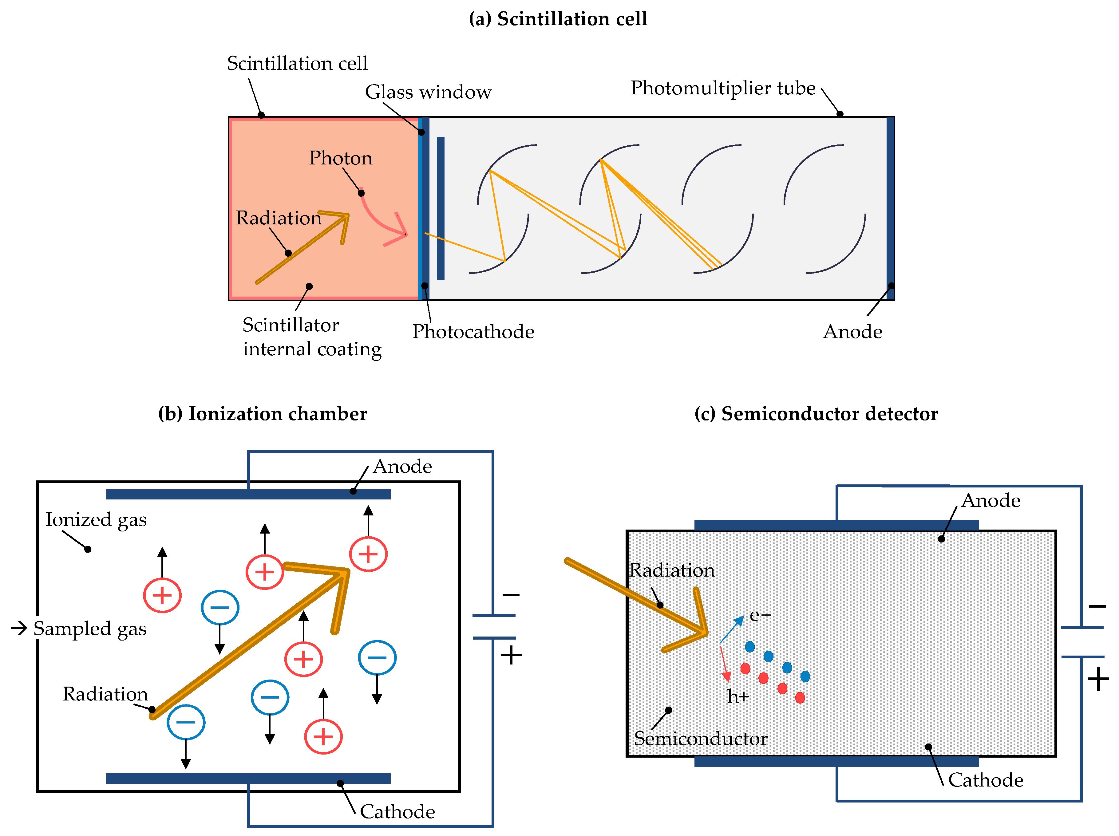
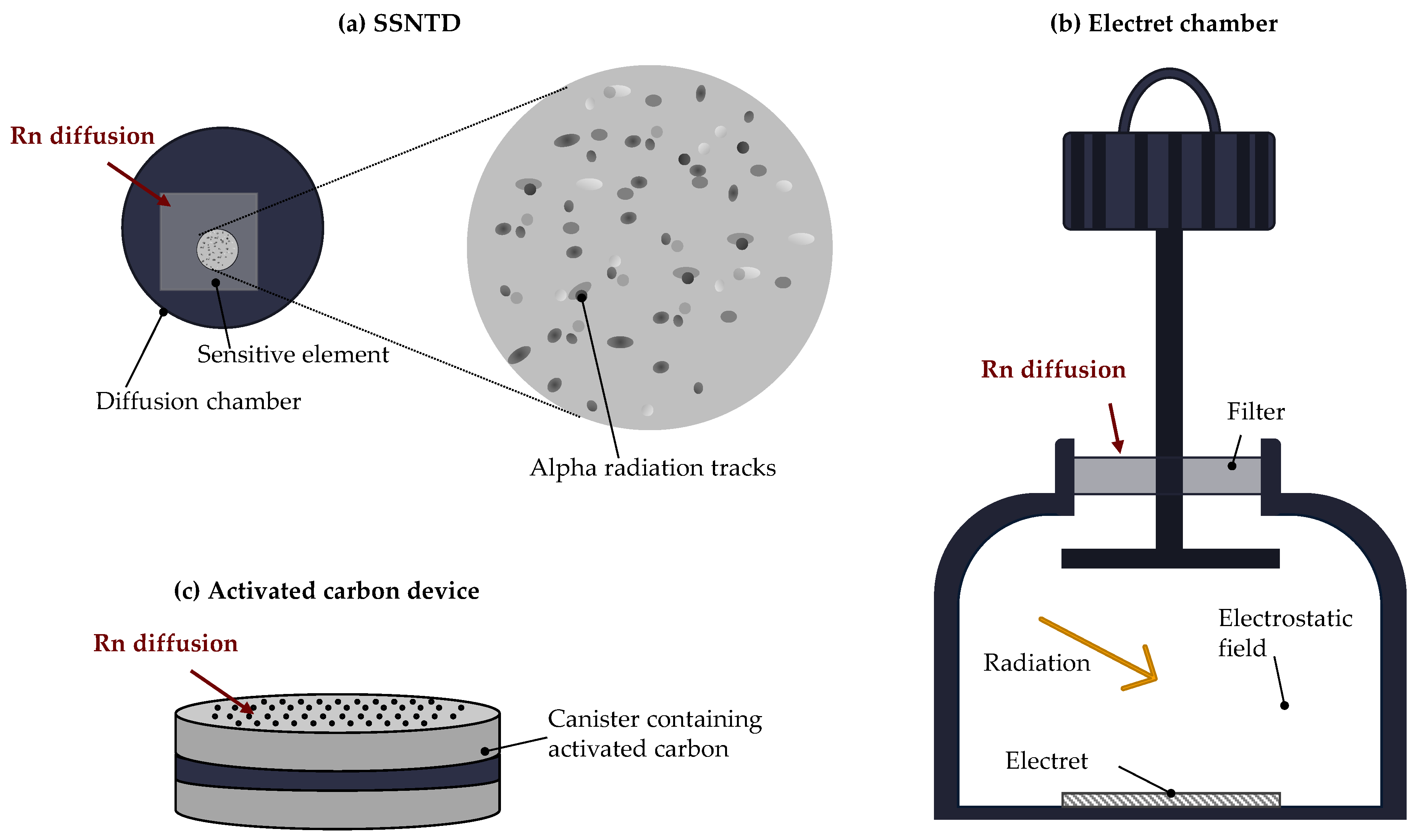
5.2.1. Soil Gas Radon Measurements

The identification and estimation of Rn activity concentration in environmental matrices typically involves procedures that utilize its alpha emitter properties. The energy of alpha particles, emitted from Rn itself or its decay products, varies between 5.5 and 7.7 MeV [43]. Two main sampling approaches are generally used to detect Rn gas: passive mode, where Rn enters the instrument through natural diffusion, and active mode, where Rn is pumped into a Rn-detecting device [125]. Furthermore, three types of Rn sampling methods can be employed: instantaneous or grab sampling, continuous sampling, and integration techniques [126]. Instantaneous techniques involve the collection of samples over a short period, such as 10 min, to be analyzed shortly thereafter, usually within 4 h [127]. For each sample, it provides a single activity concentration value, valid for the specific conditions at the time of the survey. It can be performed on-site using a portable instrument that allows for the sampling and quick measurement of Rn activity concentration, or by taking samples in special containers to be later analyzed in specialized laboratories [128]. The detectors commonly used for this type of application are scintillation cells, ionization chambers, and semiconductor detectors. The signals are then converted into measurable pulses using appropriate processing electronics and algorithms. Measuring Rn or Rn progeny continuously involves simultaneous sampling and analysis, providing real-time results. This is particularly useful in situations where Rn activity concentrations can change significantly and rapidly. Measurement intervals typically range from 15 to 60 min, with useful results obtained after 2 to 3 h of continuous sampling and counting. Continuous Rn and Rn progeny monitors offer real-time Rn concentration data and can measure other parameters such as temperature, pressure, or humidity. Additionally, they allow for the analysis of time trends in real-time recorded parameters. However, these instruments are expensive and complex, requiring trained personnel to operate [127]. Integrating methods provide a single Rn activity concentration value that is representative of the average activity concentration over an observation period that can range from a few days to a year [51]. Integrated measurement with passive instrumentation is usually the most commonly used.

Other criteria that differentiate them are the applicability of field measurements, portability, and cost. Various technologies can be used to measure Rn in the different configurations mentioned above. Some examples of this technology with further details are given below, classified according to the type of sampling.

Active mode measurement methods, such as scintillation cells, ionization chambers, and semiconductor detectors, are typically utilized for field measurements or in situations where continuous measurement is required.

Scintillation cells (Figure 5a), also known as Lucas cells [129], are hermetically sealed containers that are filled with a sample containing the Rn gas, or the emanated Rn from water, to be analyzed. Rn gas can be collected inside the cell either using a pre-evacuated scintillation cell or flow mode. A filter is typically included to prevent dust and Rn decay products from entering the cell and affecting the counting process [126]. The internal coating of the scintillation cell is made of silver-activated zinc sulfide ZnS, which scintillates when alpha particles resulting from Rn decay strike it. Light photons are produced when alpha particles from Rn and its decay products interact with zinc sulfide in the cell [130]. The photons can then be counted using, for instance, a photomultiplier tube, and the resulting data, usually expressed in terms of Bq m⁻³, are sent to a digital data logger.

Ionization chambers (Figure 5b) typically comprise cylindrical volumes with metal walls and two electrodes: one consisting of the walls themselves and the other of a central wire acting as an anode. An electrical field is established between the electrodes. Filtered air is either allowed to diffuse into the chamber or is pumped in. Electrons are produced through the ionization of sampled air by alpha particles of Rn and its decay products [131]. The charged electret collects the ions, and the charge decreases as a function of the integrated Rn activity over the exposed time. The measurement can be performed either by measuring the total ionization in the chamber or by counting the pulses caused by individual alpha particles separately [51]. These instruments are adequate for high-precision measurements but are usually complex and expensive [132].

Semiconductor detectors (Figure 5c) use a semiconductor material (usually silicon) that is sensitive to the presence of charged particles, in particular transforming alpha radiation into an electrical signal. Charged particles passing through the device generate electron–lacuna pairs and are collected by the electrodes, creating ionization currents [133]. The detector material converts the stored energy into an electrical signal from the electrostatic collection of Rn and its decay products. The sample gas is introduced into the detector chamber either passively (by diffusion) or actively (by pumping). These detectors’ major advantage is their ability to distinguish each incoming alpha particle in terms of emitted energy [126].

Passive instrumentation is commonly used for integrated measurement. Commonly used devices for different fields and applications are solid-state nuclear track detectors (SSNTDs), electret ionization chambers, or activated carbon. Although passive instrumentation has not been widely used, SSNTDs are the most extensively studied and tested method in the field of Rn deficit technique. Additionally, new carbon-based devices have also been tested (see Section 5.2.3).

SSNTD (Figure 6a) relies on the use of materials that are sensitive to alpha radiation, which causes damage to the chemical bonds of the material itself, leaving traces known as tracks [134]. These traces are distinguishable from the intrinsic irregularity and damage to the crystal structure and can be made visible under an optical microscope by chemically treating them with a basic solution [135]. The traces can then be analyzed using optical or electronic techniques. SSNTDs are suitable for long-term measurements and provide a measure of the average Rn activity concentration during the exposure period [132]. Several sensitive materials are used for this purpose, such as LR-115 (cellulose nitrate), CR-39 (polyallydiglycol carbonate), and Makrofol (polycarbonate) [136].

Electret ionization chambers (Figure 6b) consist of an electrically conducting chamber with an electret at the bottom and a filtered inlet at the top. The electret is usually a piece of polytetrafluoroethylene that has been electrically charged and processed to exhibit a stable charge. It collects ions generated by Rn and its associated decay products inside the chamber, causing a drop in the surface voltage of the electret [137]. The detector acts as a time integrator of Rn exposure.

The method of activated carbon (Figure 6c) utilizes passive diffusion to collect Rn from the environment by adsorbing it onto activated charcoal, which has an affinity for many gases, including Rn. The collector, containing charcoal with adsorbed Rn and decay products, is sealed after exposure. Counting is typically performed at least 3 h after exposure to ensure equilibrium between Rn and its progenitors [127]. The measure can be performed employing two detection methods: gamma counting and liquid scintillation. Rn activity concentration can be determined by counting gamma rays emitted by Rn progeny during the decay process [138], using a standard gamma-ray spectrometer equipped with high-purity germanium HPGe or sodium iodide doped with thallium NaI (Tl) detectors [51]. Liquid scintillation uses the high solubility of Rn in aromatic solvents such as toluene. To analyze charcoal exposed to Rn using this technology, it is mixed with a liquid scintillation cocktail in which Rn readily dissolves. The sample is stored for three hours before the measurement to allow for equilibrium between Rn and its decay products [139]. The activity of Rn and its progeny is determined by detecting the photon count from the scintillation fluid.

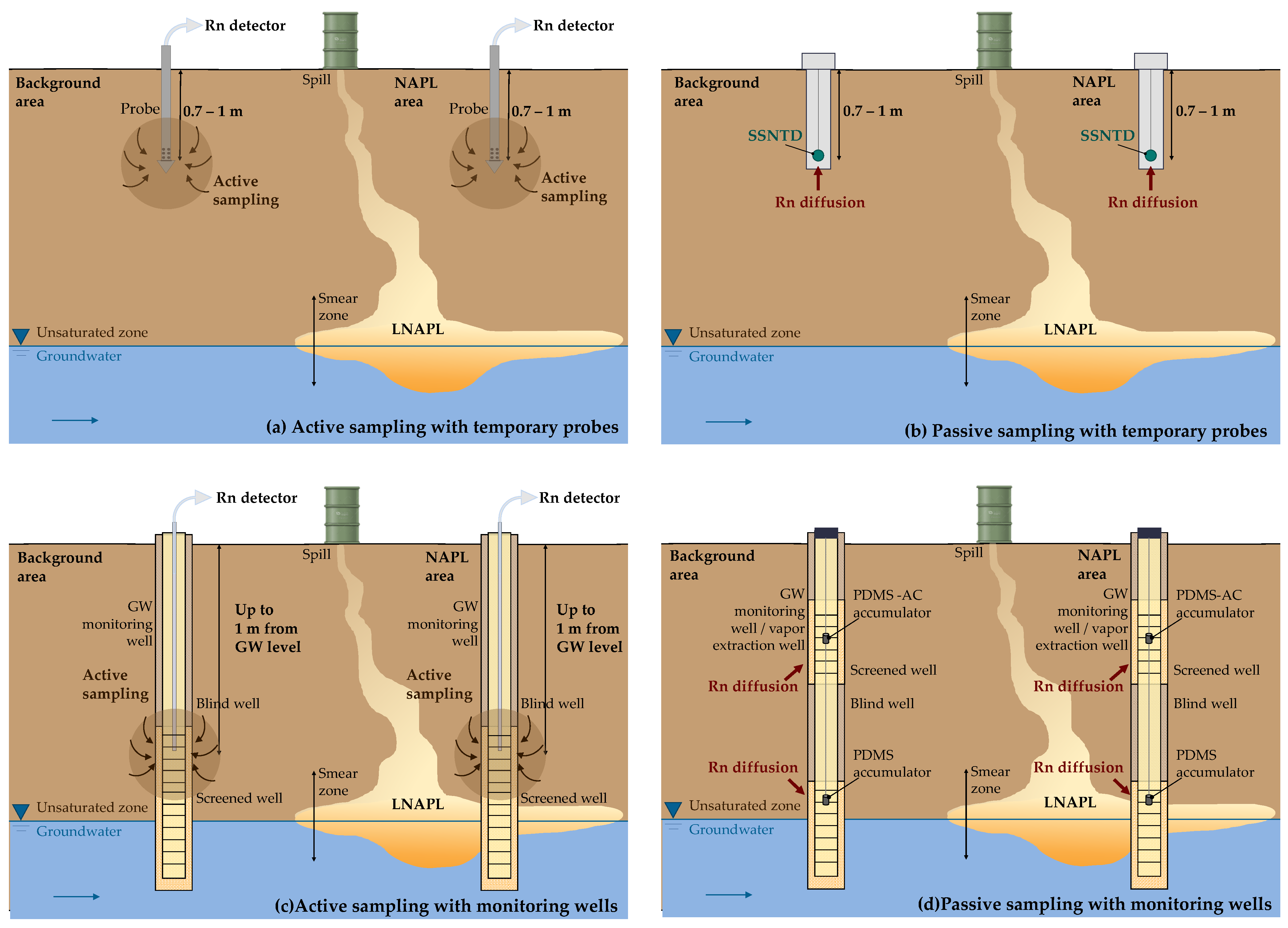
5.2.2. Soil Gas Applications Using Active Sampling

One of the most frequently used methods for soil gas sampling involves the utilization of temporary soil gas probes (refer to Figure 7a). These probes are constructed from stainless-steel hollow bars with free, pointed bottom ends (“lost” tips). The probes are then installed to a depth of 0.7–1 m, either manually or using tools such as electric drills [19,23,25,29,115]. This depth range is typical when using temporary probes and is mainly defined by the necessity to sample soil gas at a depth that will be minimally affected by atmospheric variables, such as temperature, atmospheric pressure, and wind velocity. However, it is important to take into account the feasibility of temporary probe installation [140], since the penetration of a hollow probe to depths beyond those mentioned above may not be practical, depending on the properties of the soil or the existence of subsurface facilities [29]. Schubert et al. [19,117] conducted some field experiments to test the use of soil gas Rn activity concentration to detect LNAPL contamination using this configuration. In particular, three sites contaminated with petroleum and kerosene with the presence of floating LNAPL were chosen. These sites had previously been investigated to delineate the LNAPL plumes. For the Rn surveys, a grid of soil gas sampling points was installed at each site using temporary soil gas probes. Soil gas samples were collected at a depth of 70 cm, and Rn activity concentrations were measured using a pulsed ionization chamber mobile Rn monitor. The results showed that the minimum Rn activity concentrations detected matched the respective LNAPL plumes previously traced by conventional means, highlighting the limitations related to geological complexities and the characteristic diffusion length of Rn. During the blind field test conducted by García-González et al. [29], soil gas was collected using a stainless-steel hollow probe that was inserted into the soil to a depth of 75–100 cm. Rn in soil gas was measured with a semiconductor detector. The data from eight monitoring wells have been used to determine the subsurface extent of the LNAPL plume. Despite the uncertainties associated with the map of mobile product thickness, there is a clear inverse correlation between the thickness of free product in the subsurface and Rn activity concentration in soil gas. Despite its simplicity, cost-effectiveness, and good reproducibility, the authors note that emanometry revealed some limitations during field trials, such as the need to ensure low humidity conditions to ensure good instrument performance or the potential problem of inserting the hollow probe into the ground. In a field test performed by Barbosa et al. [56], soil gas data were collected at a gas station using ten temporary soil gas probes to investigate the correlation between Rn activity and VOC concentrations in the subsurface soil. Over the entire survey area, there was no significant correlation between Rn and VOC concentrations in soil gas. However, the area near the fuel leak showed the highest VOC concentration and the lowest Rn activity. Castelluccio et al. [23] used a multi-method approach to monitor LNAPL contamination in two study areas in Italy and India. They performed soil gas Rn measurements at a depth of 80 cm using a semiconductor Rn monitor connected to a hollow probe. The Rn activity concentration was measured by counting the decay of Rn daughters after the soil gas was collected, dried, and filtered. The extent of contamination in the upper part of the unsaturated aquifers was determined by deriving the Rn deficit through a comparison with average soil Rn in reference to unpolluted areas. Additionally, residual fractions of contaminants in the vadose zone were estimated using the measurements. A direct correlation was found between the Rn deficit at shallow depths and the highest electrical resistivity at greater depths, which increases the reliability of the results of the methods. De Miguel et al. [115] used temporary soil gas probes to measure soil gas Rn through hollow rods buried 75–100 cm in the subsoil, at a site with lithological discontinuities through a blind test. Rn was measured using alpha spectroscopy monitors, following a regular sampling design with a 20 m² grid and adding some external points to assess the background Rn activity concentration in soil gas at the site. Although the soil gas Rn activity concentration was primarily influenced by the possible path of a fault and a lithologic discontinuity, the characterization of the background emission in each lithologic unit allowed for the identification of areas that may be impacted by LNAPL. Cohen et al. [59] compared the performance of multiple in situ gas measurements over soil coring for defining LNAPL source zones in the subsurface characterized by limited diffusion potential due to the presence of fine-grained soils. They used a network of gas probes at a depth of approximately 1 m and analyzed VOCs, O₂, CO₂, CH₄, and Rn, comparing the results to independent LNAPL analysis by coring at the site. Rn monitoring was conducted using scintillation vials placed under vacuum to sample soil gas from dedicated soil gas probes in the field, and a photomultiplier. The data suggested that O₂, CO₂, and CH₄ have longer diffusion lengths and provide a clearer indication of the presence of LNAPL at the site, while the migration of VOCs and Rn did not show a strong correlation with LNAPL, probably because it only occurs over short distances in such heterogeneous media. In the same study, numerical simulations were performed using a code for flow and reactive transport in variably saturated media [108] to characterize the production and transport processes of the studied gas in the vadose zone. The simulations aim to understand the role of the presence of LNAPL on gas profiles, using simplified scenarios. This modeling approach was then further explored in a following paper [60] in order to enhance the comprehension of the suitability of the Rn deficit technique in soil gas for the identification of subsurface LNAPL contamination in heterogeneous vadose zones and to determine the critical factors that affect the field implementation of the technique. The performance of the soil gas Rn deficit technique was also evaluated by Barrio-Parra et al. [25,109] at a site where a complex DNAPL mixture contaminated the soil profile. Soil gas samples were collected using a syringe and introduced into a previously vacuumed ionization chamber. Samples were collected using hollow rods at two depths (0.8 m and 1.7 m) and purged to prevent dilution effects due to atmospheric air. Rn measurements were performed using a pulse ionization detector. A negative spatial correlation was found between soil gas Rn activity concentrations and organic contaminant levels in the top layers of the soil profile, indicating that the method correctly identified surface contaminant hotspots at the site. However, the same correlations were not found for deeper contamination, which is the typical location of DNAPL in the aquifer. Therefore, according to the authors, the inability to describe the deeper vertical profile of contaminant concentration along the soil profile using only shallow soil gas samples likely invalidates the Rn deficit technique as a screening tool for deep DNAPL accumulations. Barrio-Parra et al. [109] developed a numerical multilayer model of Rn production–partitioning–diffusion in unsaturated porous media. They also included a laboratory protocol to obtain site-specific input parameters for the model. The model predictions were compared with field information obtained from sampling campaigns measuring soil gas Rn at a site where the vadose zone was affected by the presence of a DNAPL mixture. The model successfully predicted the vertical profile of soil gas Rn activity concentrations, including the effects of soil moisture, which varied due to water table fluctuations and soil temperature.

In other contexts where soil gas monitoring may be necessary, such as in vapor intrusion assessments, it is common to install dedicated soil gas probes for extended periods of time. One option for installing these probes is by excavating a pre-drilled hole to the desired depth and installing a PVC or stainless-steel pipe inside. Alternatively, it is possible to use direct push drilling methods to insert the pipe directly into the ground [141]. The borehole is filled with coarse sand at the bottom and sealed with bentonite for the rest of its length [142], and the head of the probe is usually provided with a gas-tight connection that can be directly attached to the sampling hose. For the application of the soil gas Rn deficit technique, this setup usually does not provide substantial benefits in data quality over the temporary probe sampling method. De Miguel et al. [26] proposed an adaptation of the conventional method using PVC pipes installed directly in the soil, designed with a perforated base for the entry of soil gas into the probe, and fitted with an airtight top valve that can be opened for the purge of the system and the sampling phase. This configuration was applied in a blind field test, conducted to evaluate the performance of the Rn deficit technique for a complex mixture of organic contaminants. The results obtained with this approach were comparable to those obtained in other studies that used temporary probes. For the area investigated by De Miguel et al. [26], the pollution hotspots inferred from the Rn campaigns aligned with the analytical data on the location of the pollution source zones obtained from traditional sampling campaigns. However, the authors identified the variation of Rn activity concentrations with diurnal changes in ground-level air temperature and the maximum depth of the investigation as limitations to the applicability of the technique. According to the authors, for an effecting application of the Rn deficit technique, the influence of temperature can be accounted for and minimized by averaging replicated measurements during different days. Regarding the maximum depth of investigation, the authors concluded that variations in soil gas Rn activity concentrations are spatially correlated with changes in soil contamination only if the depth of the sampling point is within the maximum diffusion radius of Rn from the source zone. This latter limitation was considered statistically significant only if no significant advective or co-advective transport of Rn in soil gas is assumed at the site. Mattia et al. [27] measured Rn in soil gas by extracting it from two vapor extraction wells from a Soil Vapor Extraction (SVE) system, at different depths, and analyzing the samples in the laboratory using a semiconductor detector connected in a closed loop. Rn deficit observed in soil gas was used together with the more abundant Rn data obtained from groundwater sampling from the wells at the site, to identify the location of residual LNAPL. Soil gas samples were not used for quantitative estimations due to their lower abundance compared to groundwater samples.

With respect to the specific aspect of the vertical distance between soil gas probes for Rn measurements and the LNAPL source zone in the subsoil, an alternative method was proposed [101] for the use of the soil gas Rn deficit technique, utilizing the headspace of groundwater monitoring wells (Figure 7b). This protocol is based on the use of portable active Rn detectors for the rapid determination of Rn soil gas activity in the smear zone, which allows for measurements to be made in the unsaturated soil where residual LNAPL is typically present. A first evaluation of the applicability of this method was performed at two Italian sites where an accidental release into the subsurface of gasoline and diesel from fuel tanks occurred. Despite the limited number of tests conducted, the results indicate that measuring Rn in the headspace of monitoring wells is a reasonably viable option for measuring Rn near the LNAPL source zone.

5.2.3. Soil Gas Applications Using Passive Sampling

Another approach is to use solid-state nuclear track detectors (Figure 7c). The detectors are exposed for a variable period (days or weeks) before being analyzed to determine the average Rn activity for the exposure period. Schubert et al. [55] conducted a soil gas Rn survey using solid-state nuclear track detectors LR-115. The purpose was to evaluate the efficiency of these instruments as a cost-effective method for the application of the technique. At the field site, the detectors were exposed for 8 days inside samplers buried in the soil at a depth of 70 cm. After exposure, all detectors were etched with a NaOH solution to reveal the alpha particle impacts as etching tracks. The resulting Rn distribution pattern indicated areas with concentrations at least 90% lower than the local background level, spatially matching the LNAPL contamination present in the subsurface. Mateus and Pecequilo [58] evaluated the Rn deficit technique in soil gas using passive detection methodology with CR-39 solid-state nuclear track detectors. The method was tested by placing the detectors inside special diffusion chambers within 1 m long PVC tubes buried in the soil. The detector was suspended inside the PVC pipe at a depth of 70 cm, together with a permeable bag containing silica gel, to prevent moisture, which can complicate alpha particle interactions. After 20 days of exposure, the detectors were removed and analyzed to obtain track densities and the relative Rn activity concentrations. For the monitoring points assumed as contaminated locations, Rn activity concentrations diminished in a range from 92% to 98% when compared with the results for the non-contaminated areas. The authors discovered that the monitoring point with the lowest Rn activity concentration was located outside the LNAPL area estimated with classical environmental investigation techniques. However, during additional excavation in the area, evidence of oil-impregnated soil was found, confirming the results of the Rn monitoring technique.

Briganti et al. [54] conducted a study to evaluate the feasibility of determining the vertical distribution of Rn at various soil depths to detect LNAPL contamination, using the passive Rn accumulator proposed by Voltaggio et al. [143] (Figure 7d). These passive accumulators, made of polydimethylsiloxane (PDMS) mixed with activated carbon (AC), were designed to measure Rn in both soil gas and groundwater due to the water-impermeable (PDMS) and Rn-adsorbing (AC) properties of the two materials. The accumulators were inserted at varying depths into monitoring wells and left inside for two weeks to absorb ambient Rn that diffuses within the material. After the recovery process, each sample was counted in the laboratory using a high-resolution gamma spectrometer equipped with an HPGe detector. These experimental results appear to be consistent with the presence of residual LNAPL in the vadose zone, also indicated by detected peaks of VOC. From this initial field test, the authors found that PDMS-AC passive accumulators yielded positive results for environmental Rn sampling.

Based on the results presented in the above studies, passive samplers appear to be an adequate and less expensive tool for determining Rn distribution patterns in the upper soil.

6. Conclusions, Limitations, and Future Research

The Rn deficit technique has emerged as a useful method for the initial assessment of sites impacted by complex organic compound mixtures associated with the occurrence of non-aqueous phases. The results obtained with different applications of the technique, in terms of identifying the location of NAPL contamination hotspots, were often consistent with those obtained using standard direct and indirect exploration techniques or with historical information about the site’s contamination sources, e.g., [22,25,28,29,51,53,111]. Compared to conventional investigation tools such as drilling and soil groundwater sampling and analysis, Rn measurements can provide nearly real-time results with the potential for much higher spatial density at a lower cost [26,51]. Furthermore, the method can detect the presence of LNAPL in the subsurface even when it exists in residual phase [24], which is usually more challenging since, unlike the free product, it cannot be detected by conventional monitoring of groundwater wells at the site. Similarly, it may be useful to distinguish areas of pure dissolved phase plume from areas of actual separate phase presence [112,119].

Although the setups described in the previous section have yielded positive results, there are still some limitations to the applicability of the soil gas Rn deficit technique. Published work on the subject has identified different categories of limitations, mostly associated with the fluctuations of Rn activity in the soil over time and space and the distance between the soil gas measurement point and LNAPL depth. Modeling efforts have been utilized to evaluate the performance of the use of Rn monitoring for subsurface LNAPL detection under different site-specific conditions, either by considering the more typical case of diffusive-only transport in soil gas or by including advective transport in the evaluations [21,25,60,106,107]. The results of these works provided suggestions for both field workers and researchers on the practical application of the technique and the interpretation of the resulting data. However, analytical models may be limited in their ability to model complex scenarios due to the assumptions required. For future research opportunities, new numerical modeling developments could be beneficial in these circumstances and may help to identify potential areas for improvement over current field approaches. Nevertheless, the key parameters identified by the modeling work also resulted from the field investigations conducted with different configurations.

Different authors [19,24,26,59,112,117] highlighted that Rn activity concentrations in the field may be affected by the geochemical, lithological, granulometric, and mineralogical characteristics of the soil. This may be due to the uneven distribution of ²²⁶Ra, from which Rn originates, in the soil, and to variations in the emanation mechanism based on soil characteristics. Specifically, the concentration of ²²⁶Ra can vary significantly among different rock types. For instance, granites (acidic igneous rocks), some types of bituminous shales, and phosphate rocks typically have higher average radioactivity concentrations [61]. Therefore, variations in Rn activity concentrations may arise due to heterogeneities in lithostratigraphic units, and not necessarily be related to the presence of LNAPL in the subsoil. As an example, Rn measurements were performed in soil gas in a site characterized by a significant heterogeneity of the subsurface and did not find a clear pattern in Rn concentrations above the LNAPL zone [59]. Additionally, the characteristics of the soil matrix, such as grain size and permeability affect both Rn emanation and soil gas transport, and, therefore, its activity concentration in soil gas along soil profiles. These latter aspects can also complicate the application of the method in identifying the appropriate area to use as the reference Rn background value for the site for estimating the deficit. The development of strategies that consider the heterogeneity of the soil matrix is crucial for the future advancement of the technique. To this end, additional field investigations in a wide range of geological settings are necessary to increase the availability of field data, and thereby increase its applicability in different scenarios.

Another important consideration in the application of this technique is the possible temporal variability of Rn measurements. Soil gas behavior in the shallowest soil layers, specifically those less than 1 m deep, is affected by weather conditions such as temperature, atmospheric pressure, and wind speed [86]. Concerning pressure, a consistent Rn variability was not observed with the diurnal variation in barometric pressure [25]. It has been assumed in various applications that measuring Rn down to a depth of 75–100 cm can minimize the influence of atmospheric factors [25,29,55,115]. However, temperature was found to have a significant effect on Rn concentrations in surface soils to varying degrees depending on the sampling and measurement methods used [25,26,144]. It was also observed that the vertical temperature gradient in the soil may have an influence on depths around 1 m, which is typical of the method’s application [25]. If not properly accounted for, the thermal effect can result in a confounding effect in the interpretation of Rn deficits. To avoid this effect on Rn concentration measurements in surface soil gas, it was recommended [25] to use the arithmetic mean of the data set for each campaign. Passive instruments, such as SSNTDs, could be considered as an alternative option for Rn measurement, as they integrate Rn activity concentrations over a longer exposure time, flattening out some of the possible variability. It is important to account for the temperature effect when comparing the results of different field campaigns, as seasonal and diurnal variations may also be relevant [145,146]. Future research could aim to determine if the observed variability is predictable and to develop new monitoring methods that account for temporal fluctuations in Rn. This could potentially improve the consistency and reliability of the technique results.

Although the soil gas Rn method has shown positive qualitative results in most tested cases for identifying zones with LNAPL presence in the subsurface, there are still few studies related to quantifying LNAPL contamination using this technique in the unsaturated zone [22,23]. In fact, the quantification of the extent of the contamination requires a greater knowledge of subsurface characteristics, the nature and composition of the contaminant, and overall site-specific parameters. In this context, an important aspect to consider is the variability of the partition coefficient value depending on the composition of the LNAPL and the possible degradation phenomena it may have undergone over time [110].

Another factor that can impact the effectiveness of the Rn deficit method in the vadose zone is the distance of the Rn measurement point from the LNAPL source zone. In the case of deep contamination or of inhibited Rn transport, e.g., for a low soil permeability or higher water content, there may be a decrease in the characteristic gas diffusion length of Rn, thus restricting the capability of the Rn deficit technique [19,21,22,26,115,147]. For instance, Schubert et al. [117] described a positive outcome of the method to delineate an area with mobile subsurface kerosene but pointed out the difficulties associated with the lithological complexity and the reduced Rn diffusion distance. A further example is the outcome of different field campaigns performed by Barrio Parra et al. [25], which demonstrated a clear correlation between low Rn activities and the major contaminant concentrations in the upper soil. However, there was no evidence of the same correlations for the contamination found in the underlying soil layers. It should be noted that some authors [26,115] have suggested that the existence of a fractured system can promote Rn transport in the subsurface through possible co-advective transport mechanisms, thus modifying soil gas and Rn dynamics in the subsurface. To directly measure soil gas Rn activity at the source zone, headspace Rn measurements in groundwater monitoring wells have been proposed and tested as an alternative to permanent or temporary soil gas probes, with successful qualitative outcomes [101].

Based on the available information and knowledge summarized in this overview, it is believed that the method has the potential to be used as a rapid, inexpensive, minimally invasive, and sustainable approach to subsurface LNAPL investigation, even in the presence of residual phase, for an initial screening during the site characterization, as well as for LNAPL monitoring over time and during remediation activities. Despite the method’s promise for qualitative identification, challenges such as soil matrix heterogeneity (with both passive and active instrumentation) and temporal variations in Rn emissions (with active instrumentation) have been recognized to affect quantitative evaluations. In this view, future research, and collaboration among researchers and industry professionals, should aim to refine both established and emerging methods under diverse site-specific conditions, addressing limitations associated with soil matrix heterogeneity and temporal Rn variability to improve the reliability and applicability of the technique for the assessment of LNAPL contamination. Furthermore, improving the technique with advanced and smart-oriented approaches, as well as refining current methodologies to enhance their sustainability, can help reduce environmental impacts and more efficiently manage concerns related to LNAPL contamination.

References

1. US EPA. Ground Water Issue: Light Nonaqueous Phase Liquids; US EPA: Washington, DC, USA, 1995. [Google Scholar]
2. Alden, D.F.; García-Rincón, J.; Rivett, M.O.; Wealthall, G.P.; Thomson, N.R. Complexities of Petroleum Hydrocarbon Contaminated Sites. In Advances in the Characterisation and Remediation of Sites Contaminated with Petroleum Hydrocarbons; García-Rincón, J., Gatsios, E., Lenhard, R.J., Atekwana, E.A., Naidu, R., Eds.; Environmental Contamination Remediation and Management; Springer International Publishing: Cham, Switzerland, 2024; pp. 1–19. ISBN 978-3-031-34447-3. [Google Scholar]
3. CL:AIRE. An Illustrated Handbook of LNAPL Transport and Fate in the Subsurface; CL:AIRE: London, UK, 2014. [Google Scholar]
4. Sweeney, R.E.; Ririe, G.T. Small Purge Method to Sample Vapor from Groundwater Monitoring Wells Screened across the Water Table. Groundw. Monit. Remediat. 2017, 37, 51–59. [Google Scholar] [CrossRef]
5. US EPA. A Decision-Making Framework for Cleanup of Sites Impacted with Light Non-Aqueous Phase Liquids (LNAPL); US EPA: Washington, DC, USA, 2004. [Google Scholar]
6. ITRC. LNAPL Site Management: LCSM Evolution, Decision Process, and Remedial Technologies; ITRC: Washington, DC, USA, 2018. [Google Scholar]
7. ITRC. Implementing Advanced Site Characterization Tools; ITRC: Washington, DC, USA, 2019. [Google Scholar]
8. Bertolla, L.; Porsani, J.L.; Soldovieri, F.; Catapano, I. GPR-4D Monitoring a Controlled LNAPL Spill in a Masonry Tank at USP, Brazil. J. Appl. Geophys. 2014, 103, 237–244. [Google Scholar] [CrossRef]
9. McCall, W.; Christy, T.M.; Pipp, D.A.; Jaster, B.; White, J.; Goodrich, J.; Fontana, J.; Doxtader, S. Evaluation and Application of the Optical Image Profiler (OIP) a Direct Push Probe for Photo-Logging UV-Induced Fluorescence of Petroleum Hydrocarbons. Environ. Earth Sci. 2018, 77, 374. [Google Scholar] [CrossRef]
10. Shao, S.; Guo, X.; Gao, C. Fresh Underground Light Non-Aqueous Liquid (LNAPL) Pollution Source Zone Monitoring in an Outdoor Experiment Using Cross-Hole Electrical Resistivity Tomography. Environ. Sci. Pollut. Res. 2019, 26, 18316–18328. [Google Scholar] [CrossRef] [PubMed]
11. Teramoto, E.H.; Isler, E.; Polese, L.; Baessa, M.P.M.; Chang, H.K. LNAPL Saturation Derived from Laser Induced Fluorescence Method. Sci. Total Environ. 2019, 683, 762–772. [Google Scholar] [CrossRef] [PubMed]
12. García-Rincón, J.; Gatsios, E.; Rayner, J.L.; McLaughlan, R.G.; Davis, G.B. Laser-Induced Fluorescence Logging as a High-Resolution Characterisation Tool to Assess LNAPL Mobility. Sci. Total Environ. 2020, 725, 138480. [Google Scholar] [CrossRef] [PubMed]
13. Lu, Q.; Wang, Y.; Li, H. GPR Attribute Analysis for the Detection of LNAPL Contaminated Soils. IOP Conf. Ser. Earth Environ. Sci. 2021, 660, 012033. [Google Scholar] [CrossRef]
14. Meng, J.; Dong, Y.; Xia, T.; Ma, X.; Gao, C.; Mao, D. Detailed LNAPL Plume Mapping Using Electrical Resistivity Tomography inside an Industrial Building. Acta Geophys. 2022, 70, 1651–1663. [Google Scholar] [CrossRef]
15. Mineo, S. Groundwater and Soil Contamination by LNAPL: State of the Art and Future Challenges. Sci. Total Environ. 2023, 874, 162394. [Google Scholar] [CrossRef] [PubMed]
16. St. Germain, R. High-Resolution Delineation of Petroleum NAPLs. In Advances in the Characterisation and Remediation of Sites Contaminated with Petroleum Hydrocarbons; García-Rincón, J., Gatsios, E., Lenhard, R.J., Atekwana, E.A., Naidu, R., Eds.; Environmental Contamination Remediation and Management; Springer International Publishing: Cham, Switzerland, 2024; pp. 213–286. ISBN 978-3-031-34447-3. [Google Scholar]
17. Rao, P.S.C.; Annable, M.D.; Kim, H. NAPL Source Zone Characterization and Remediation Technology Performance Assessment: Recent Developments and Applications of Tracer Techniques. J. Contam. Hydrol. 2000, 45, 63–78. [Google Scholar] [CrossRef]
18. Semprini, L.; Hopkins, O.S.; Tasker, B.R. Laboratory, Field and Modeling Studies of Radon-222 as a Natural Tracer for Monitoring NAPL Contamination. Transp. Porous Media 2000, 38, 223–240. [Google Scholar] [CrossRef]
19. Schubert, M.; Freyer, K.; Treutler, H.-C.; Weiß, H. Using the Soil Gas Radon as an Indicator for Ground Contamination by Non-Aqueous Phase-Liquids. J. Soils Sediments 2001, 1, 217–222. [Google Scholar] [CrossRef]
20. Davis, B.M.; Istok, J.D.; Semprini, L. Push–Pull Partitioning Tracer Tests Using Radon-222 to Quantify Non-Aqueous Phase Liquid Contamination. J. Contam. Hydrol. 2002, 58, 129–146. [Google Scholar] [CrossRef] [PubMed]
21. Höhener, P.; Surbeck, H. Radon-222 as a Tracer for Nonaqueous Phase Liquid in the Vadose Zone: Experiments and Analytical Model. Vadose Zone J. 2004, 3, 1276–1285. [Google Scholar] [CrossRef]
22. Schubert, M. Using Radon as Environmental Tracer for the Assessment of Subsurface Non-Aqueous Phase Liquid (NAPL) Contamination—A Review. Eur. Phys. J. Spec. Top. 2015, 224, 717–730. [Google Scholar] [CrossRef]
23. Castelluccio, M.; Agrahari, S.; De Simone, G.; Pompilj, F.; Lucchetti, C.; Sengupta, D.; Galli, G.; Friello, P.; Curatolo, P.; Giorgi, R.; et al. Using a Multi-Method Approach Based on Soil Radon Deficit, Resistivity, and Induced Polarization Measurements to Monitor Non-Aqueous Phase Liquid Contamination in Two Study Areas in Italy and India. Environ. Sci. Pollut. Res. 2018, 25, 12515–12527. [Google Scholar] [CrossRef]
24. Briganti, A.; Tuccimei, P.; Voltaggio, M.; Carusi, C.; Galli, G.; Lucchetti, C. Assessing Methyl Tertiary Butyl Ether Residual Contamination in Groundwater Using Radon. Appl. Geochem. 2020, 116, 104583. [Google Scholar] [CrossRef]
25. Barrio-Parra, F.; Izquierdo-Díaz, M.; Díaz-Curiel, J.; De Miguel, E. Field Performance of the Radon-Deficit Technique to Detect and Delineate a Complex DNAPL Accumulation in a Multi-Layer Soil Profile. Environ. Pollut. 2021, 269, 116200. [Google Scholar] [CrossRef] [PubMed]
26. De Miguel, E.; Barrio-Parra, F.; Izquierdo-Díaz, M.; Fernández, J.; García-González, J.E.; Álvarez, R. Applicability and Limitations of the Radon-Deficit Technique for the Preliminary Assessment of Sites Contaminated with Complex Mixtures of Organic Chemicals: A Blind Field-Test. Environ. Int. 2020, 138, 105591. [Google Scholar] [CrossRef] [PubMed]
27. Mattia, M.; Tuccimei, P.; Ciotoli, G.; Soligo, M.; Carusi, C.; Rainaldi, E.; Voltaggio, M. Combining Radon Deficit, NAPL Concentration, and Groundwater Table Dynamics to Assess Soil and Groundwater Contamination by NAPLs and Related Attenuation Processes. Appl. Sci. 2023, 13, 12813. [Google Scholar] [CrossRef]
28. Fan, K.; Kuo, T.; Han, Y.; Chen, C.; Lin, C.; Lee, C. Radon Distribution in a Gasoline-Contaminated Aquifer. Radiat. Meas. 2007, 42, 479–485. [Google Scholar] [CrossRef]
29. García-González, J.E.; Ortega, M.F.; Chacón, E.; Mazadiego, L.F.; Miguel, E.D. Field Validation of Radon Monitoring as a Screening Methodology for NAPL-Contaminated Sites. Appl. Geochem. 2008, 23, 2753–2758. [Google Scholar] [CrossRef]
30. Yoon, Y.Y.; Koh, D.C.; Lee, K.Y.; Cho, S.Y.; Yang, J.H.; Lee, K.K. Using 222Rn as a Naturally Occurring Tracer to Estimate NAPL Contamination in an Aquifer. Appl. Radiat. Isot. 2013, 81, 233–237. [Google Scholar] [CrossRef] [PubMed]
31. CL:AIRE. Site Characterisation in Support of Monitored Natural Attenuation of Fuel Hydrocarbons and MTBE in a Chalk Aquifer in Southern England; CL:AIRE Case Study Bulletin, CSB 1; CL:AIRE: London, UK, 2002. [Google Scholar]
32. Tsai, Y.-J.; Chou, Y.-C.; Wu, Y.-S.; Lee, C.-H. Noninvasive Survey Technology for LNAPL-Contaminated Site Investigation. J. Hydrol. 2020, 587, 125002. [Google Scholar] [CrossRef]
33. Lenhard, R.J.; Parker, J.C. Estimation of Free Hydrocarbon Volume from Fluid Levels in Monitoring Wells. Groundwater 1990, 28, 57–67. [Google Scholar] [CrossRef]
34. Kemblowski, M.W.; Chiang, C.Y. Hydrocarbon Thickness Fluctuations in Monitoring Wells. Groundwater 1990, 28, 244–252. [Google Scholar] [CrossRef]
35. Atteia, O.; Palmier, C.; Schäfer, G. On the Influence of Groundwater Table Fluctuations on Oil Thickness in a Well Related to an LNAPL Contaminated Aquifer. J. Contam. Hydrol. 2019, 223, 103476. [Google Scholar] [CrossRef] [PubMed]
36. Arato, A.; Wehrer, M.; Biró, B.; Godio, A. Integration of Geophysical, Geochemical and Microbiological Data for a Comprehensive Small-Scale Characterization of an Aged LNAPL-Contaminated Site. Environ. Sci. Pollut. Res. 2014, 21, 8948–8963. [Google Scholar] [CrossRef] [PubMed]
37. Biosca, B.; Arévalo-Lomas, L.; Barrio-Parra, F.; Díaz-Curiel, J. Application and Limitations of Time Domain-Induced Polarization Tomography for the Detection of Hydrocarbon Pollutants in Soils with Electro-Metallic Components: A Case Study. Environ. Monit. Assess. 2020, 192, 115. [Google Scholar] [CrossRef] [PubMed]
38. Mercer, J.W.; Cohen, R.M. A Review of Immiscible Fluids in the Subsurface: Properties, Models, Characterization and Remediation. J. Contam. Hydrol. 1990, 6, 107–163. [Google Scholar] [CrossRef]
39. Karimi Askarani, K.; Sale, T.; Palaia, T. Natural Source Zone Depletion of Petroleum Hydrocarbon NAPL. In Advances in the Characterisation and Remediation of Sites Contaminated with Petroleum Hydrocarbons; García-Rincón, J., Gatsios, E., Lenhard, R.J., Atekwana, E.A., Naidu, R., Eds.; Environmental Contamination Remediation and Management; Springer International Publishing: Cham, Switzerland, 2024; pp. 113–138. ISBN 978-3-031-34447-3. [Google Scholar]
40. Setarge, B.; Danzer, J.; Klein, R.; Grathwohl, P. Partitioning and Interfacial Tracers to Characterize Non-Aqueous Phase Liquids (NAPLs) in Natural Aquifer Material. Phys. Chem. Earth Part B Hydrol. Oceans Atmos. 1999, 24, 501–510. [Google Scholar] [CrossRef]
41. Annable, M.D.; Rao, P.S.C.; Hatfield, K.; Graham, W.D.; Wood, A.L.; Enfield, C.G. Partitioning Tracers for Measuring Residual NAPL: Field-Scale Test Results. J. Environ. Eng. 1998, 124, 498–503. [Google Scholar] [CrossRef]
42. US EPA. Cost and Performance Report for LNAPL Characterization and Remediation Partition Interwell Tracer Testing (PITT) and Rapid Optical Screening Tool (ROSTTM). In Characterization and Evaluation of the Feasibility of Surfactant Enhanced Aquifer Remediation (SEAR) at the Chevron Cincinnati Facility; US EPA: Hooven, OH, USA, 2005. [Google Scholar]
43. Stacks, A.M. Radon: Geology, Environmental Impact and Toxicity Concerns; Nova Publishers: Hauppauge, NY, USA, 2015; p. 280. ISBN 978-1-63463-777-0. [Google Scholar]
44. Rösch, F. The Basics of Nuclear Chemistry and Radiochemistry: An Introduction to Nuclear Transformations and Radioactive Emissions. In Radiopharmaceutical Chemistry; Lewis, J.S., Windhorst, A.D., Zeglis, B.M., Eds.; Springer International Publishing: Cham, Switzerland, 2019; pp. 27–61. ISBN 978-3-319-98947-1. [Google Scholar]
45. Gutiérrez Villanueva, J.-L.G. Radon Concentrations in Air, Soil, and Water in a Granitic Area: Instrumental Development and Measurements. Doctoral Dissertation, Universidad de Valladolid, Valladolid, Spain, 2008. [Google Scholar]
46. NRC. Risk Assessment of Radon in Drinking Water; National Research Council (US) Committee on Risk Assessment of Exposure to Radon in Drinking Water; National Academies Press (US): Washington, DC, USA, 1999; ISBN 978-0-309-06292-3. [Google Scholar]
47. Nazaroff, W.; Moed, B.; Sextro, R.; Revzan, K.; Nero, A. Factors Influencing Soil as a Source of Indoor Radon: Framework for Assessing Radon Source Potential; Lawrence Berkeley National Laboratory: Berkeley, CA, USA, 1989; p. LBL-20645. [Google Scholar]
48. WHO. Guidelines for Drinking-Water Quality, 3rd ed.; WHO: Geneva, Switzerland, 2008; Volume 1. [Google Scholar]
49. Baskaran, M. Radon: A Tracer for Geological, Geophysical and Geochemical Studies; Springer: Basel, Switzerland, 2016; ISBN 978-3-319-21329-3. [Google Scholar]
50. Quindos Poncela, L.S.; Sainz Fernandez, C.; Fuente Merino, I.; Gutierrez Villanueva, J.L.; Gonzalez Diez, A. The Use of Radon as Tracer in Environmental Sciences. Acta Geophys. 2013, 61, 848–858. [Google Scholar] [CrossRef]
51. Sukanya, S.; Noble, J.; Joseph, S. Application of Radon (222Rn) as an Environmental Tracer in Hydrogeological and Geological Investigations: An Overview. Chemosphere 2022, 303, 135141. [Google Scholar] [CrossRef] [PubMed]
52. Hunkeler, D.; Hoehn, E.; Höhener, P.; Zeyer, J. 222Rn as a Partitioning Tracer To Detect Diesel Fuel Contamination in Aquifers:  Laboratory Study and Field Observations. Environ. Sci. Technol. 1997, 31, 3180–3187. [Google Scholar] [CrossRef]
53. Schubert, M.; Lehmann, K.; Paschke, A. Determination of Radon Partition Coefficients between Water and Organic Liquids and Their Utilization for the Assessment of Subsurface NAPL Contamination. Sci. Total Environ. 2007, 376, 306–316. [Google Scholar] [CrossRef]
54. Briganti, A.; Voltaggio, M.; Rainaldi, E.; Carusi, C. Vertical Light Non-Aqueous Phase Liquid (LNAPL) Distribution by Rn Prospecting in Monitoring Wells. Environ. Monit. Assess. 2024, 196, 19. [Google Scholar] [CrossRef] [PubMed]
55. Schubert, M.; Pena, P.; Balcazar, M.; Meissner, R.; Lopez, A.; Flores, J.H. Determination of Radon Distribution Patterns in the Upper Soil as a Tool for the Localization of Subsurface NAPL Contamination. Radiat. Meas. 2005, 40, 633–637. [Google Scholar] [CrossRef]
56. Barbosa, E.Q.; Galhardi, J.A.; Bonotto, D.M. The Use of Radon (Rn-222) and Volatile Organic Compounds in Monitoring Soil Gas to Localize NAPL Contamination at a Gas Station in Rio Claro, São Paulo State, Brazil. Radiat. Meas. 2014, 66, 1–4. [Google Scholar] [CrossRef]
57. De Simone, G.; Galli, G.; Lucchetti, C.; Tuccimei, P. Using Natural Radon as a Tracer of Gasoline Contamination. Procedia Earth Planet. Sci. 2015, 13, 104–107. [Google Scholar] [CrossRef]
58. Mateus, C.; Pecequilo, B.R.S. Preliminary Results of NAPL Contamination in a Disused Industry in the City of São Paulo, Brazil, by Radon Evaluation with CR-39 Detectors. In Proceedings of the INAC 2015: International Nuclear Atlantic Conference, Sao Paulo, SP, Brazil, 4–9 October 2015. [Google Scholar]
59. Cohen, G.J.V.; Jousse, F.; Luze, N.; Höhener, P.; Atteia, O. LNAPL Source Zone Delineation Using Soil Gases in a Heterogeneous Silty-Sand Aquifer. J. Contam. Hydrol. 2016, 192, 20–34. [Google Scholar] [CrossRef] [PubMed]
60. Cohen, G.J.V.; Bernachot, I.; Su, D.; Höhener, P.; Mayer, K.U.; Atteia, O. Laboratory-Scale Experimental and Modelling Investigations of 222Rn Profiles in Chemically Heterogeneous LNAPL Contaminated Vadose Zones. Sci. Total Environ. 2019, 681, 456–466. [Google Scholar] [CrossRef] [PubMed]
61. Nazaroff, W.W. Radon Transport from Soil to Air. Rev. Geophys. 1992, 30, 137–160. [Google Scholar] [CrossRef]
62. UNSCEAR. Sources and Effects of Ionizing Radiation; UNSCEAR: Vienna, Austria, 1977. [Google Scholar]
63. Lombardi, S.; Voltattorni, N. Rn, He and CO2 Soil Gas Geochemistry for the Study of Active and Inactive Faults. Appl. Geochem. 2010, 25, 1206–1220. [Google Scholar] [CrossRef]
64. Davidson, J.R.J.; Fairley, J.; Nicol, A.; Gravley, D.; Ring, U. The Origin of Radon Anomalies along Normal Faults in an Active Rift and Geothermal Area. Geosphere 2016, 12, 1656–1669. [Google Scholar] [CrossRef]
65. Tanner, A.B. Radon Migration in the Ground: A Supplementary Review; US Geological Survey: Reston, VA, USA, 1980; pp. 5–56. [Google Scholar]
66. Sakoda, A.; Ishimori, Y.; Yamaoka, K. A Comprehensive Review of Radon Emanation Measurements for Mineral, Rock, Soil, Mill Tailing and Fly Ash. Appl. Radiat. Isot. 2011, 69, 1422–1435. [Google Scholar] [CrossRef] [PubMed]
67. Hassan, N.M.; Hosoda, M.; Ishikawa, T.; Sorimachi, A.; Sahoo, S.K.; Tokonami, S.; Fukushi, M. Radon Migration Process and Its Influence Factors; Review. Jpn. J. Health Phys. 2009, 44, 218–231. [Google Scholar] [CrossRef]
68. Krishnaswami, S.; Seidemann, D.E. Comparative Study of 222Rn, 40Ar, 39Ar and 37Ar Leakage from Rocks and Minerals: Implications for the Role of Nanopores in Gas Transport through Natural Silicates. Geochim. Cosmochim. Acta 1988, 52, 655–658. [Google Scholar] [CrossRef]
69. Markkanen, M.; Arvela, H. Radon Emanation from Soils. Radiat. Prot. Dosim. 1992, 45, 269–272. [Google Scholar] [CrossRef]
70. Stranden, E.; Kolstad, A.K.; Lind, B. The Influence of Moisture and Temperature on Radon Exhalation. Radiat. Prot. Dosim. 1984, 7, 55–58. [Google Scholar] [CrossRef]
71. Iskandar, D.; Yamazawa, H.; Iida, T. Quantification of the Dependency of Radon Emanation Power on Soil Temperature. Appl. Radiat. Isot. 2004, 60, 971–973. [Google Scholar] [CrossRef] [PubMed]
72. NCRP. Measurement of Radon and Radon Daughters in Air; National Council on Radiation Protection and Measurements: Bethesda, MD, USA, 1988. [Google Scholar]
73. Perrier, F.; Richon, P.; Sabroux, J.-C. Temporal Variations of Radon Concentration in the Saturated Soil of Alpine Grassland: The Role of Groundwater Flow. Sci. Total Environ. 2009, 407, 2361–2371. [Google Scholar] [CrossRef] [PubMed]
74. Lee, K.Y.; Yoon, Y.Y.; Ko, K.S. Determination of the Emanation Coefficient and the Henry’s Law Constant for the Groundwater Radon. J. Radioanal. Nucl. Chem. 2010, 286, 381–385. [Google Scholar] [CrossRef]
75. Schery, S.D.; Whittlestone, S. Desorption of Radon at the Earth’s Surface. J. Geophys. Res. 1989, 94, 18297–18304. [Google Scholar] [CrossRef]
76. Penman, H.L. Gas and Vapour Movements in the Soil: I. The Diffusion of Vapours through Porous Solids. J. Agric. Sci. 1940, 30, 437–462. [Google Scholar] [CrossRef]
77. Penman, H.L. Gas and Vapour Movements in the Soil: II. The Diffusion of Carbon Dioxide through Porous Solids. J. Agric. Sci. 1940, 30, 570–581. [Google Scholar] [CrossRef]
78. Marshall, T.J. A Relation Between Permeability and Size Distribution of Pores. J. Soil Sci. 1958, 9, 1–8. [Google Scholar] [CrossRef]
79. Millington, R.J.; Quirk, J.P. Permeability of Porous Solids. Trans. Faraday Soc. 1961, 57, 1200–1207. [Google Scholar] [CrossRef]
80. Millington, R.J.; Shearer, R.C. Diffusion in Aggregated Porous Media. Soil Sci. 1971, 111, 372–378. [Google Scholar] [CrossRef]
81. Strong, K.P.; Levins, D.M. Effect of Moisture Content on Radon Emanation from Uranium Ore and Tailings. Health Phys. 1982, 42, 27–32. [Google Scholar] [CrossRef] [PubMed]
82. Tanner, A.B. Radon Migration in the Ground: A Review. In Natural Radiation Environment; University of Chicago Press: Chicago, IL, USA, 1964; pp. 161–190. [Google Scholar]
83. Broecker, W.S.; Peng, T.H. Gas Exchange Rates between Air and Sea1. Tellus 1974, 26, 21–35. [Google Scholar] [CrossRef]
84. Chauhan, R.P.; Nain, M.; Kant, K. Radon Diffusion Studies through Some Building Materials: Effect of Grain Size. Radiat. Meas. 2008, 43, S445–S448. [Google Scholar] [CrossRef]
85. Hillel, D. Introduction to Soil Physics; Academic Press: Cambridge, MA, USA, 1982; ISBN 978-0-08-091869-3. [Google Scholar]
86. Scanlon, B.R.; Nicot, J.P.; Massmann, J.W. Soil Gas Movement in Unsaturated Systems. Soil Phys. Companion 2002, 389, 297–341. [Google Scholar]
87. Auer, L.H.; Rosenberg, N.D.; Birdsell, K.H.; Whitney, E.M. The Effects of Barometric Pumping on Contaminant Transport. J. Contam. Hydrol. 1996, 24, 145–166. [Google Scholar] [CrossRef]
88. Forde, O.N.; Cahill, A.G.; Beckie, R.D.; Mayer, K.U. Barometric-Pumping Controls Fugitive Gas Emissions from a Vadose Zone Natural Gas Release. Sci. Rep. 2019, 9, 14080. [Google Scholar] [CrossRef] [PubMed]
89. Etiope, G.; Lombardi, S. Evidence for Radon Transport by Carrier Gas through Faulted Clays in Italy. J. Radioanal. Nucl. Chem. 1995, 193, 291–300. [Google Scholar] [CrossRef]
90. Čeliković, I.; Pantelić, G.; Vukanac, I.; Nikolić, J.K.; Živanović, M.; Cinelli, G.; Gruber, V.; Baumann, S.; Ciotoli, G.; Poncela, L.S.Q.; et al. Overview of Radon Flux Characteristics, Measurements, Models and Its Potential Use for the Estimation of Radon Priority Areas. Atmosphere 2022, 13, 2005. [Google Scholar] [CrossRef]
91. Qi, S.; Luo, J.; O’Connor, D.; Wang, Y.; Hou, D. A Numerical Model to Optimize LNAPL Remediation by Multi-Phase Extraction. Sci. Total Environ. 2020, 718, 137309. [Google Scholar] [CrossRef] [PubMed]
92. Man, J.; Wang, G.; Chen, Q.; Yao, Y. Investigating the Role of Vadose Zone Breathing in Vapor Intrusion from Contaminated Groundwater. J. Hazard. Mater. 2021, 416, 126272. [Google Scholar] [CrossRef] [PubMed]
93. Cavelan, A.; Golfier, F.; Colombano, S.; Davarzani, H.; Deparis, J.; Faure, P. A Critical Review of the Influence of Groundwater Level Fluctuations and Temperature on LNAPL Contaminations in the Context of Climate Change. Sci. Total Environ. 2022, 806, 150412. [Google Scholar] [CrossRef]
94. Cunningham, R.E.; Williams, R.J.J. Diffusion in Gases and Porous Media; Springer: Boston, MA, USA, 1980; ISBN 978-1-4757-4985-4. [Google Scholar]
95. Yang, C.; Wang, Z.; Hollebone, B.P.; Brown, C.E.; Yang, Z.; Landriault, M. Chromatographic Fingerprinting Analysis of Crude Oils and Petroleum Products. In Handbook of Oil Spill Science and Technology; John Wiley & Sons, Ltd.: Hoboken, NJ, USA, 2014; pp. 93–163. ISBN 978-1-118-98998-2. [Google Scholar]
96. Kitto, M.E. Interrelationship of Indoor Radon Concentrations, Soil-Gas Flux, and Meteorological Parameters. J. Radioanal. Nucl. Chem. 2005, 264, 381–385. [Google Scholar] [CrossRef]
97. Zhuo, W.; Chen, B.; Li, D.; Liu, H. Reconstruction of Database on Natural Radionuclide Contents in Soil in China. J. Nucl. Sci. Technol. 2008, 45, 180–184. [Google Scholar] [CrossRef]
98. Hirao, S.; Yamazawa, H.; Moriizumi, J. Estimation of the Global 222Rn Flux Density from the Earth’s Surface. Jpn. J. Health Phys. 2010, 45, 161–171. [Google Scholar] [CrossRef]
99. López-Coto, I.; Mas, J.L.; Bolivar, J.P. A 40-Year Retrospective European Radon Flux Inventory Including Climatological Variability. Atmos. Environ. 2013, 73, 22–33. [Google Scholar] [CrossRef]
100. Andrews, J.N.; Wood, D.F. Mechanism of Radon Release in Rock Matrices and Entry into Groundwaters. Inst. Min. Met. Trans. Sect B 1972, 81, 198–209. [Google Scholar]
101. Cecconi, A.; Verginelli, I.; Baciocchi, R.; Lanari, C.; Villani, F.; Bonfedi, G. Using Groundwater Monitoring Wells for Rapid Application of Soil Gas Radon Deficit Technique to Evaluate Residual LNAPL. J. Contam. Hydrol. 2023, 258, 104241. [Google Scholar] [CrossRef] [PubMed]
102. Brost, E.J.; DeVaull, G.E. Non-Aqueous Phase Liquid (NAPL) Mobility Limits in Soil; American Petroleum Institute: Washington, DC, USA, 2000. [Google Scholar]
103. Van Der Spoel, W.H.; Van Der Graaf, E.R.; De Meijer, R.J. Diffusive Transport of Radon in a Homogeneous Column of Dry Sand. Health Phys. 1997, 72, 766–778. [Google Scholar] [CrossRef] [PubMed]
104. Van Der Spoel, W.H.; Van Der Graaf, E.R.; De Meijer, R.J. Combined Diffusive and Advective Transport of Radon in a Homogeneous Column of Dry Sand. Health Phys. 1998, 74, 48–63. [Google Scholar] [CrossRef] [PubMed]
105. Werner, D.; Höhener, P. Diffusive Partitioning Tracer Test for Nonaqueous Phase Liquid (NAPL) Detection in the Vadose Zone. Environ. Sci. Technol. 2002, 36, 1592–1599. [Google Scholar] [CrossRef] [PubMed]
106. Cecconi, A.; Verginelli, I.; Barrio-Parra, F.; De Miguel, E.; Baciocchi, R. Influence of Advection on the Soil Gas Radon Deficit Technique for the Quantification of LNAPL. Sci. Total Environ. 2023, 875, 162619. [Google Scholar] [CrossRef]
107. Cecconi, A.; Verginelli, I.; Baciocchi, R. Modeling of Soil Gas Radon as an in Situ Partitioning Tracer for Quantifying LNAPL Contamination. Sci. Total Environ. 2022, 806, 150593. [Google Scholar] [CrossRef] [PubMed]
108. Mayer, K.U.; Frind, E.O.; Blowes, D.W. Multicomponent Reactive Transport Modeling in Variably Saturated Porous Media Using a Generalized Formulation for Kinetically Controlled Reactions. Water Resour. Res. 2002, 38, 13-1–13-21. [Google Scholar] [CrossRef]
109. Barrio-Parra, F.; Hidalgo, A.; Izquierdo-Díaz, M.; Arévalo-Lomas, L.; De Miguel, E. 1D_RnDPM: A Freely Available 222Rn Production, Diffusion, and Partition Model to Evaluate Confounding Factors in the Radon-Deficit Technique. Sci. Total Environ. 2022, 807, 150815. [Google Scholar] [CrossRef] [PubMed]
110. Le Meur, M.; Cohen, G.J.V.; Laurent, M.; Höhener, P.; Atteia, O. Effect of NAPL Mixture and Alteration on 222Rn Partitioning Coefficients: Implications for NAPL Subsurface Contamination Quantification. Sci. Total Environ. 2021, 791, 148210. [Google Scholar] [CrossRef] [PubMed]
111. Wilhelm, E.; Battino, R.; Wilcock, R.J. Low-Pressure Solubility of Gases in Liquid Water. Available online: https://pubs.acs.org/doi/pdf/10.1021/cr60306a003 (accessed on 19 July 2023).
112. Schubert, M.; Paschke, A.; Lau, S.; Geyer, W.; Knöller, K. Radon as a Naturally Occurring Tracer for the Assessment of Residual NAPL Contamination of Aquifers. Environ. Pollut. 2007, 145, 920–927. [Google Scholar] [CrossRef] [PubMed]
113. Ponsin, V.; Chablais, A.; Dumont, J.; Radakovitch, O.; Höhener, P. 222Rn as Natural Tracer for LNAPL Recovery in a Crude Oil-Contaminated Aquifer. Groundw. Monit. Remediat. 2015, 35, 30–38. [Google Scholar] [CrossRef]
114. De Simone, G.; Lucchetti, C.; Pompilj, F.; Galli, G.; Tuccimei, P.; Curatolo, P.; Giorgi, R. Soil Radon Survey to Assess NAPL Contamination from an Ancient Spill. Do Kerosene Vapors Affect Radon Partition? J. Environ. Radioact. 2017, 171, 138–147. [Google Scholar] [CrossRef] [PubMed]
115. De Miguel, E.; Barrio-Parra, F.; Elío, J.; Izquierdo-Díaz, M.; García-González, J.E.; Mazadiego, L.F.; Medina, R. Applicability of Radon Emanometry in Lithologically Discontinuous Sites Contaminated by Organic Chemicals. Environ. Sci. Pollut. Res. 2018, 25, 20255–20263. [Google Scholar] [CrossRef] [PubMed]
116. Mattia, M.; Tuccimei, P.; Soligo, M.; Carusi, C. Radon as a Natural Tracer for Monitoring NAPL Groundwater Contamination. Water 2020, 12, 3327. [Google Scholar] [CrossRef]
117. Schubert, M.; Freyer, K.; Treutler, H.C.; Weiss, H. Using Radon-222 in Soil Gas as an Indicator of Subsurface Contamination by Non-Aqueous Phase-Liquids (NAPLs). Geofísica Int. 2002, 41, 433–437. [Google Scholar]
118. Davis, B.M.; Istok, J.D.; Semprini, L. Numerical Simulations of Radon as an in Situ Partitioning Tracer for Quantifying NAPL Contamination Using Push–Pull Tests. J. Contam. Hydrol. 2005, 78, 87–103. [Google Scholar] [CrossRef] [PubMed]
119. Schubert, M.; Balcázar, M.; Lopez, A.; Peña, P.; Flores, J.H.; Knöller, K. Combination of Radon and Stable Isotope Analysis as a Tool for Decision Support Concerning the Remediation of NAPL-Contaminated Sites. Isot. Environ. Health Stud. 2007, 43, 215–226. [Google Scholar] [CrossRef] [PubMed]
120. Galhardi, J.A.; Bonotto, D.M. Radon in Groundwater Contaminated by Dissolved Hydrocarbons in Santa Bárbara d’Oeste, São Paulo State, Brazil. Appl. Radiat. Isot. 2012, 70, 2507–2515. [Google Scholar] [CrossRef] [PubMed]
121. Cho, I.; Ju, Y.; Lee, S.-S.; Kaown, D.; Lee, K.-K. Characterization of a NAPL-Contaminated Site Using the Partitioning Behavior of Noble Gases. J. Contam. Hydrol. 2020, 235, 103733. [Google Scholar] [CrossRef] [PubMed]
122. Semprini, L.; Broholm, K.; McDonald, M. Radon-222 Deficit Method for Locating and Quantifying NAPL Contamination in the Subsurface. EOS Trans Am. Geophys Union 1993, 74, 299. [Google Scholar]
123. Semprini, L.; Hopkins, O.S.; Gottipati, S.; Tasker, B.R. Field, Laboratory and, Modeling Studies of Radon-222 as a Natural Tracer for Detecting NAPL Contamination in the Subsurface and Monitoring the Progress of Remediation. EOS Trans. Am. Geophys. Union 1995, 76, F276. [Google Scholar]
124. Wang, X.; Li, H.; Zhang, Y.; Qu, W.; Schubert, M. Submarine Groundwater Discharge Revealed by 222Rn: Comparison of Two Continuous on-Site 222Rn-in-Water Measurement Methods. Hydrogeol. J. 2019, 27, 1879–1887. [Google Scholar] [CrossRef]
125. Janik, M.; Ishikawa, T.; Omori, Y.; Kavasi, N. Invited Article: Radon and Thoron Intercomparison Experiments for Integrated Monitors at NIRS, Japan. Rev. Sci. Instrum. 2014, 85, 022001. [Google Scholar] [CrossRef] [PubMed]
126. Sumesh, C.G.; Jha, S.K.; Patra, A.C.; Aswal, D.K. Evolution of Analytical Methods for Radon Measurement in India. MAPAN 2024, 39, 181–192. [Google Scholar] [CrossRef]
127. George, A.C. An Overview of Instrumentation for Measuring Environmental Radon and Radon Progeny. IEEE Trans. Nucl. Sci. 1990, 37, 892–901. [Google Scholar] [CrossRef]
128. Papastefanou, C. Measuring Radon in Soil Gas and Groundwaters: A Review. 2007. Available online: http://hdl.handle.net/2122/3870 (accessed on 19 July 2023).
129. Lucas, H.F. Improved Low-Level Alpha-Scintillation Counter for Radon. Rev. Sci. Instrum. 1957, 28, 680–683. [Google Scholar] [CrossRef]
130. Sethy, N.K.; Jha, V.N.; Ravi, P.M.; Tripathi, R.M. A Simple Method for Calibration of Lucas Scintillation Cell Counting System for Measurement of 226Ra and 222Rn. J. Radiat. Res. Appl. Sci. 2014, 7, 472–477. [Google Scholar] [CrossRef]
131. Fortmann, R.C. Measurement Methods and Instrumentation. In Radon; ASTM International: West Conshohocken, PA, USA, 1993. [Google Scholar]
132. Nunes, L.J.R.; Curado, A.; Lopes, S.I. The Relationship between Radon and Geology: Sources, Transport and Indoor Accumulation. Appl. Sci. 2023, 13, 7460. [Google Scholar] [CrossRef]
133. Dalla Betta, G.-F.; Ye, J. Silicon Radiation Detector Technologies: From Planar to 3D. Chips 2023, 2, 83–101. [Google Scholar] [CrossRef]
134. Nikezic, D.; Yu, K.N. Formation and Growth of Tracks in Nuclear Track Materials. Mater. Sci. Eng. R Rep. 2004, 46, 51–123. [Google Scholar] [CrossRef]
135. Miles, J.C.H.; Sinnaeve, J. The Performance of Different Types of Etched-Track Radon Dosemeters in Two International Intercomparisons. Int. J. Radiat. Appl. Instrum. Part Nucl. Tracks Radiat. Meas. 1986, 12, 735–738. [Google Scholar] [CrossRef]
136. Gewali, J.P.; Sheron, P.; Thakur, A.; Jaishy, B. Study of Radiation Interactions in Makrofol-E and LR-115 Detectors Using SSNTD Technique. In Selected Progresses in Modern Physics; Sengupta, S., Dey, S., Das, S., Saikia, D.J., Panda, S., Podila, R., Eds.; Springer: Singapore, 2021; pp. 375–385. [Google Scholar]
137. Kotrappa, P.; Brubaker, T.; Dempsey, J.C.; Stieff, L.R. Electret Ion Chamber System for Measurement of Environmental Radon and Environmental Gamma Radiation. Radiat. Prot. Dosim. 1992, 45, 107–110. [Google Scholar] [CrossRef]
138. ISO 11665-1:2019; Measurement of Radioactivity in the Environment—Air: Radon-222—Part 1: Origins of Radon and Its Short-Lived Decay Products and Associated Measurement Methods. ISO: Geneva, Switzerland, 2019.
139. L’Annunziata, M.F. Handbook of Radioactivity Analysis; Academic Press: Cambridge, MA, USA, 2012; ISBN 978-0-12-384874-1. [Google Scholar]
140. Neznal, M.; Matolín, M.; Just, G.; Turek, K. Short-Term Temporal Variations of Soil Gas Radon Concentration and Comparison of Measurement Techniques. Radiat. Prot. Dosim. 2004, 108, 55–63. [Google Scholar] [CrossRef] [PubMed]
141. ITRC. The Use of Direct Push Well Technology for Long-Term Environmental Monitoring in Groundwater Investigations; ITRC: Washington, DC, USA, 2006. [Google Scholar]
142. CalEPA, (California Environmental Protection Agency Department of Toxic Substances Control). Advisory: Active Soil Gas Investigations; CalEPA: Sacramento, CA, USA, 2015. [Google Scholar]
143. Voltaggio, M.; Spadoni, M. Determination of 222Rn in Water by Absorption in Polydimethylsiloxane Mixed with Activated Carbon and Gamma-Ray Spectrometry: An Example Application in the Radon Budget of Paterno Submerged Sinkhole (Central Italy). Appl. Geochem. 2013, 34, 65–74. [Google Scholar] [CrossRef]
144. Schubert, M.; Schulz, H. Diurnal Radon Variations in the Upper Soil Layers and at the Soil-Air Interface Related to Meteorological Parameters. Health Phys. 2002, 83, 91–96. [Google Scholar] [CrossRef] [PubMed]
145. King, C.-Y.; Minissale, A. Seasonal Variability of Soil-Gas Radon Concentration in Central California. Radiat. Meas. 1994, 23, 683–692. [Google Scholar] [CrossRef]
146. Hutter, A.R. Spatial and Temporal Variations of Soil Gas 220Rn and 222Rn at Two Sites in New Jersey. Environ. Int. 1996, 22, 455–469. [Google Scholar] [CrossRef]
147. Castelluccio, M.; De Simone, G.; Lucchetti, C.; Moroni, M.; Salvati, F.; Tuccimei, P. A New Technique to Measure in Situ Soil Gas Permeability. J. Geochem. Explor. 2015, 148, 56–59. [Google Scholar] [CrossRef]
Figure 1. 238U decay series. Only the main decays are shown. Gamma emitters are not indicated.
Sustainability 16 03317 g001
Figure 2. Scheme of Rn emanation phenomenon. Cases C and D represent the emanation phenomena. Cases A and B non-emanation. The black dots indicate the starting point of Rn generation, from 226Ra decay. The red arrows represent an indication of the recoil range, not in scale (after [67]).
Sustainability 16 03317 g002
Figure 3. Conceptual representation of the behavior of Rn in the subsurface, illustrating the reduction in Rn activity (expressed in % of the local background activity) expected in the LNAPL-affected area of the subsoil (LNAPL zone), due to the Rn partitioning in LNAPL, compared to the higher Rn activity in the unaffected area (background zone). The figure also includes two illustrations at the soil porosity level, which show the mechanisms of Rn emanation and partitioning (between the gas phase, aqueous phase, and LNAPL, if present), both in the background zone and in the LNAPL zone (after Schubert et al. [19]).
Sustainability 16 03317 g003
Figure 4. Theoretical relationship between Rn deficit and LNAPL saturation, from Equation (19), for sandy soil in the vadose zone both in the background and LNAPL area, for two different LNAPL compositions characterized by different LNAPL/gas partition coefficients, typical of a gasoline (kN/g = 9.8) and diesel composition (kN/g = 15.2), according to Schubert et al. [53] (see also Table 5).
Sustainability 16 03317 g004
Figure 5. Schematics of technologies that can be used to detect Rn in soil gas by active sampling: a scintillation cell coupled with a photomultiplier tube (a), an ionization chamber (b), and a semiconductor detector (c).
Sustainability 16 03317 g005
Figure 6. Schematics of technologies that can be used to detect Rn in soil gas by passive sampling: solid-state nuclear track detector (a), electret ionization chamber (b), and activated carbon devices (c).
Sustainability 16 03317 g006
Figure 7. Schematic of soil gas Rn sampling methods for the application of the soil gas Rn deficit technique: active sampling using temporary probes (a), passive sampling using solid-state nuclear track detectors (b), active sampling using the headspace of groundwater monitoring wells (c), and passive sampling using PDMS-AC accumulators in vapor/groundwater wells (d).
Sustainability 16 03317 g007