Article

Analysis of the Factors Influencing the Spatial Distribution of PM2.5 Concentrations (SDG 11.6.2) at the Provincial Scale in China

1
College of Geomatics and Geoinformation, Guilin University of Technology, Guilin 541006, China
2
International Research Center of Big Data for Sustainable Development Goals, Beijing 100094, China
3
Key Laboratory of Digital Earth Science, Aerospace Information Research Institute, Chinese Academy of Sciences, Beijing 100094, China
*
Author to whom correspondence should be addressed.
Sustainability 2024, 16(8), 3394; https://doi.org/10.3390/su16083394
Submission received: 3 March 2024 / Revised: 13 April 2024 / Accepted: 15 April 2024 / Published: 18 April 2024
(This article belongs to the Special Issue Win-Win Strategies for Climate Resilience and Air Pollution Control)

Abstract

:
This study investigated the spatiotemporal characteristics and influencing factors of PM2.5 concentrations at the provincial scale in China. The findings indicate significant spatial autocorrelation, with notable high–high agglomerations in East and North China and mixed patterns in the northwest. The spatial Durbin model (SDM) with fixed effects, validated through comprehensive tests, was utilized to analyze data on 31 provincial scale regions from 2000 to 2020, addressing spatial autocorrelation and ensuring model reliability. The research delved into the effects of 21 variables on PM2.5 concentrations, identifying synergistic and trade-off effects among environmental and socioeconomic indicators. Environmental measures like vegetation protection and sulfur dioxide emission reduction correlate with lower PM2.5 levels, whereas economic growth and transport volume often align with increased pollution. The analysis reveals regional variances in these effects, suggesting the need for region-specific policies. The study underscores the intricate relationship between environmental policies, economic development, and air quality, advocating for an integrated approach to air quality improvement. It highlights the necessity of balancing industrial growth with environmental sustainability and suggests targeted, region-specific strategies to combat PM2.5 pollution effectively. This study offers crucial insights for policymakers, emphasizing that enhancing air quality requires comprehensive strategies that encompass environmental, economic, and technological dimensions to foster sustainable development.

1. Introduction

Particulate matter 2.5 (PM2.5) constitutes a form of inhalable particulate matter pervasive in the atmospheric milieu, exerting a pronounced impact on human health through its association with respiratory, cardiovascular, and even dementia diseases [1,2,3]. Beyond its health ramifications, PM2.5 adversely affects vegetation growth and soil and water quality, thereby disrupting ecological balance, biodiversity, and contributing to climate change [4], impacting the economic and social development [5]. Consequently, the United Nations has officially designated PM2.5 as a key indicator within the framework of Sustainable Development Goals, specifically identified as SDG 11.6.2 [6].
Over the years, research has primarily focused on the meteorological factors responsible for the formation of PM2.5 [7,8] and its health impacts [3]. However, in recent years, there has been an increasing attention on the influence of socioeconomic factors [9]. Amid ongoing urbanization and industrialization, a combination of socioeconomic factors including industry, transportation, energy consumption, agriculture, combustion, and vegetation collectively influences localized PM2.5 levels [10,11]. Studies show that PM2.5 concentrations, characterized by its spatial attributes, exhibit a distinct degree of spatial heterogeneity [12]. For example, some research findings underscore the exacerbating impact of urbanization on air pollution, with economic urbanization exhibiting a particularly heightened influence on PM2.5 compared to land-based and population-based urbanization [13]. The correlation between China’s PM2.5 levels and economic development aligns with the environmental Kuznets curve (EKC) hypothesis, depicting an inverted U-shaped relationship with per capita GDP [14,15]. Furthermore, scholarly investigations reveal that green technological innovation, foreign investment, and expanded green vegetation areas are crucial in reducing PM2.5 concentration in both local and adjacent areas [16,17]. In China, a provincial-scale study indicates that economic activity is still the main factor to promote the increase of PM2.5 emissions, but its effect decreases [18]. Moreover, PM2.5 is influenced not only by various local factors but also by meteorological conditions such as air diffusion, leading to inter-regional air quality impacts and demonstrating a pronounced spatial correlation [19].
Many models have been used to analysis these factors of PM2.5 concentrations, such as the correlation analysis method [12], machine learning method [20], geographical detector [21,22,23], spatial econometric model (SEM) [24], geographically weighted regression model [25,26,27], spatial regression model [28], land-use regression model [29], and other models [30]. This study focuses on the spatiotemporal differentiation characteristics of PM2.5 at provincial scale in China and investigates the spatial spillover effect intensity of potential socioeconomic factors affecting PM2.5 concentrations across different provincial units. Among the above models, SEMs are highlighted as key in addressing issues of spatial heterogeneity, spillover effects, and their influencing factors. Scholars have employed the spatial error model (SEM) to study the heterogeneous impact of the secondary industry on PM2.5 [31], and the spatial Durbin model(SDM) to calculate the effect of urbanization on PM2.5 concentrations [32]. Furthermore, SEMs have been utilized to discover that the deployment and usage of natural gas pipelines can effectively mitigate PM2.5 concentrations [33]. Current research primarily employs traditional spatial weight matrices such as contiguity, economic, inverse distance, and nested matrices [34], focusing on the overall calculation of the spatial spillover effect of independent variables on dependent variables, yet lacking a quantitative analysis within regions. Therefore, to quantitatively calculate the spatial spillover effects of PM2.5 and its potential influencing factors among multiple factors and across several provinces in China, this study iteratively reduces the traditional inverse distance matrix, retaining the spatial distance weights between a single region and other regions [35]. Based on the new inverse distance matrix, the study calculates the spatial spillover effect values of multiple indicators between provinces on PM2.5 and conducts an analysis. This refined approach enables a detailed analysis of the spatial spillover effects of PM2.5 and its influencing factors at the provincial scale in China, providing robust support for the governance of air pollution and the promotion of sustainable development practices.
This manuscript is structured as follows. Section 2 details the data and methodology, covering data collection, preprocessing, and the steps to construct the spatial inverse distance matrix, as well as the implementation of Moran’s I test and the SDM. Section 3 delves into the empirical findings regarding the spatial spillover effects of PM2.5, and analyses conducted from the perspectives of indicators and provinces. It identifies the directions of the spillover effects of various provinces and influencing factors on PM2.5. We also tried to analyze the reasons for the occurrence of trade-off effects by focusing on the most significant influencing factors and provinces with apparent spillover effects. In Section 4, we summarize the experimental results and discuss their limitations. Additionally, some policy recommendations are proposed.

2. Data and Methods

2.1. Data Selection and Preprocessing

This study utilized statistical panel data from 2000 to 2020, covering 31 provincial-scale administrative regions in China (excluding Hong Kong, Macao, and Taiwan). The data originate from several authoritative sources, including the National Statistical Yearbook, China Environmental Statistical Yearbook, China Energy Statistical Yearbook, and information from the Ministry of Civil Affairs of the People’s Republic of China. In this study, the concentration of PM2.5 (SDG 11.6.2) was selected as the dependent variable. To identify the factors influencing PM2.5 levels, we meticulously selected a suite of explanatory variables based on their potential impact. This selection process was informed by a thorough review of relevant literature and the invaluable insights of experts in the field. Our methodical approach ensured the inclusion of the most pertinent factors affecting PM2.5 concentrations, establishing a robust foundation for further analysis. Due to the accessibility of the data, the variables we have selected, while not fully aligned with the specific nuances of the official United Nations SDG indicators, can to a certain extent represent the corresponding SDG indicators or targets. Consequently, we annotated each variable with the SDG indicators it supports. We ultimately selected 21 explanatory variables, with Table 1 presenting a detailed list of these indicators. In this table, a positive designation in the Direction column signifies advancement towards a more sustainable world, while a negative designation implies a trajectory that is antithetical to the attainment of sustainable development goals. For example, an increased “industrial water reuse rate” denotes a positive shift towards sustainability, thus the direction for this indicator is deemed positive. In contrast, a higher concentration of PM2.5 is detrimental to progressing towards a sustainable world; hence, the direction for this indicator is considered negative.
For the incomplete portions of the data, which do not exceed 5% for any given year, linear interpolation was employed to fill in the gaps [36]. Furthermore, to mitigate the effects of different dimensions of statistical data and outliers on the results, the original data were subjected to min-max normalization after trimming the extreme values at the 2.5% level [37]. Additionally, the direction of the negative indicator was adjusted to facilitate the analysis of the experimental result, as detailed in Formulas (1) and (2). Table 2 presents the descriptive analysis results of the normalized data, including the number of observations, mean, and standard deviation. Among the 22 variables, SDG 15.4 (protecting mountain ecology) exhibits the largest standard deviation of 29.52, while SDG 11.3.1 (land consumption) has the lowest standard deviation of 15.87. Generally, the normalized variable data show minimal fluctuation.
The forward normalization formula used was:
X = X X m i n X m a x X m i n × 100
The inverse normalization formula used was:
X = X m a x X X m a x X m i n × 100
In (1) and (2), X is original data of any given variable, Xmax and Xmin represent the 2.5% maximum and 2.5% minimum value of the variable. X′ is the normalized result of X.
To assess whether there is a multicollinearity problem between variable data, which would interfere with the experimental results, this study calculated the variance inflation factor (VIF) for each variable.
V I F = 1 ( 1 R 2 )
In Formula (3), R2 represents the correlation coefficient between this variable and other independent variables [38]. VIF can quantify how much the variance of an independent variable is inflated due to its correlation with other independent variables [38]. A VIF value of 10 or greater typically indicates significant multicollinearity among variables [38,39]. Table 2 presents the VIF of each variable studied in the last column, with the maximum value recorded at 5.76. This suggests that there is no significant multicollinearity among the variables selected for this experiment.

2.2. Method

2.2.1. Spatial Moran Index

The multi-year local Moran index can be used to assess the presence of spatial autocorrelation and to detect changes in its autocorrelation state over time [40,41]. For the i-th region, the local Moran index Ii is defined as follows:
I i = x i x ¯ S 2 j = 1 n w i j x j x ¯ ,   a n d   i j
S 2 = 1 n i = 1 n x i x ¯ 2  
In Formulas (4) and (5), n represents the total number of spatial regions of the research variable, xi represents the variable value of the i-th region, xj represents the variable value of the j-th region, x ¯ represents the average value of all variable values, w i j is the spatial weight matrix, and S2 represents the sample variance.
When I i > 0 , it indicates the presence of positive spatial correlation, typically manifested as either a high–high agglomeration (areas with high values surrounded by areas with high values) or a low–low agglomeration (areas with low values surrounded by areas with low values); conversely, when I i < 0 , it indicates negative spatial correlation, which is manifested as either a low–high agglomeration (areas with low values are surrounded by areas with high values) or a high–low agglomeration (areas with high values are surrounded by areas with low values).

2.2.2. Spatial Econometric Models (SEMs)

This study used SEMs to study spatial spillover effects. The currently popular SEMs include the spatial Durbin model (SDM), spatial lag model (SLM), and spatial error model (SEM), et al. The SDM studies the variable relationship between adjacent observation areas by processing spatially weighted spatial panel data. The formula of the SDM model is as follows [42,43]:
y = λ W y + X β + W X δ + ε
In (6), y is the explained variable, X represents the explanatory variable, W is the spatial weight matrix, and λ is the spatial regression coefficient for the dependent variable, quantifying the influence of neighboring values of (y). β represents the regression coefficient of the independent variable within the region, reflecting how changes in (X) influence (y) locally. δ is the spatial regression coefficient of the independent variable, capturing the impact of neighboring values of (X) on (y). ε represents the error term; λ W y represents the influence of dependent variables from adjacent areas. X β represents the influence of independent variables in this area, W X δ represents the influence of independent variables from adjacent areas. When λ 0 , β 0 , δ = 0 , the model is identified as SLM; when λ = 0 , β 0 ,   δ 0 , it is classified as SEM [43].
The spatial weight matrix plays an important role in spatial econometric models, particularly in studying spatial spillover effects. Typical spatial weight matrices include proximity matrix, inverse distance matrix, economic matrix, and nested (economic, distance) matrix. Due to the significant distance-related characteristics of PM2.5 spatial overflow, this study adopted an inverse distance weight matrix. Additionally, to capture the differentiated spatial distribution characteristics of PM2.5 across various provincial scale regions, 31 inverse distance weight matrices were constructed for the 31 provincial administrative units in the study. Each matrix was uniquely modified to focus solely on the spatial relationships between a given area (i) and other areas, ensuring that weights between non-focal areas were zero [35]. This modification was crucial for accurately calculating the spatial overflow relationships between area (i) and other areas, as detailed in Formula (7).
W i j = 0 w 1 i 0 w i 1 0 w i n 0 w n i 0

2.3. Model Validity Test

2.3.1. Lagrange Multiplier Test

The Lagrange multiplier test (LM test) is used to determine the presence of spatial autocorrelation in the data, which informs the applicability of spatial econometric models. The test operates under the null hypothesis that there is no serial correlation in the data residual, versus the alternative hypothesis of p-order autocorrelation [44]. When the significance level value of the statistic is less than 0.05, the null hypothesis should be rejected. indicating autocorrelation and the suitability of SEMs. Conversely, acceptance of the null hypothesis suggests an absence of autocorrelation, and SEMs are not recommended. Formula (8) calculates the LM test statistic, where T represents the time period, R ¯ u 2 is the goodness of fit for the model with explanatory variables, and R ¯ u r 2 includes both explanatory variables and individual random effects. The LM test was used in this study to preliminarily determine the suitability of the data for spatial econometric modeling.
L M = T × R ¯ u 2 R ¯ u r 2

2.3.2. Hausman Test

The Hausman test is employed to evaluate and compare the estimation results of two distinct models, characterized by either fixed or random parameters. The foundational null hypothesis posits that both the random effects model and the fixed effects model yield consistent estimates concerning the systematic error term, indicating an absence of systematic difference in their parameter estimates [45]. When the significance level attains a value of p < 0.05 or p < 0 [46], the null hypothesis is consequently rejected, prompting the adoption of fixed effects in the model. Otherwise, the null hypothesis is accepted and random effects are used. The Hausman statistic, calculated as Formula (9), where β ^ R E and β ^ F E represent the estimated outcomes of the random effects model and the fixed effects model, respectively, guides the decision on whether to adopt fixed or random effects in the model. This methodology was integral to this study’s approach to model selection between fixed and random effects.
H = ( β ^ R E β ^ F E )   [ Var ( β ^ R E β ^ F E ) ] 1 ( β ^ R E β ^ F E )

2.3.3. Likelihood Ratio Test

The likelihood ratio test (LR test) is a statistical test method commonly used to compare the adequacy of two models under different constraints. The null hypothesis asserts estimated likelihood function values from the unconstrained and constrained models are substantially equivalent [47]. When the significance value of p < 0.05 is achieved, preference is given to the constrained model; otherwise the unconstrained model is favored. In this study, the LR test was applied to assess the efficacy of model selection involving individual, time, and dual fixed effects, as well as to determine whether SDM would reduce to SLM and SEM.

3. Results and Analysis

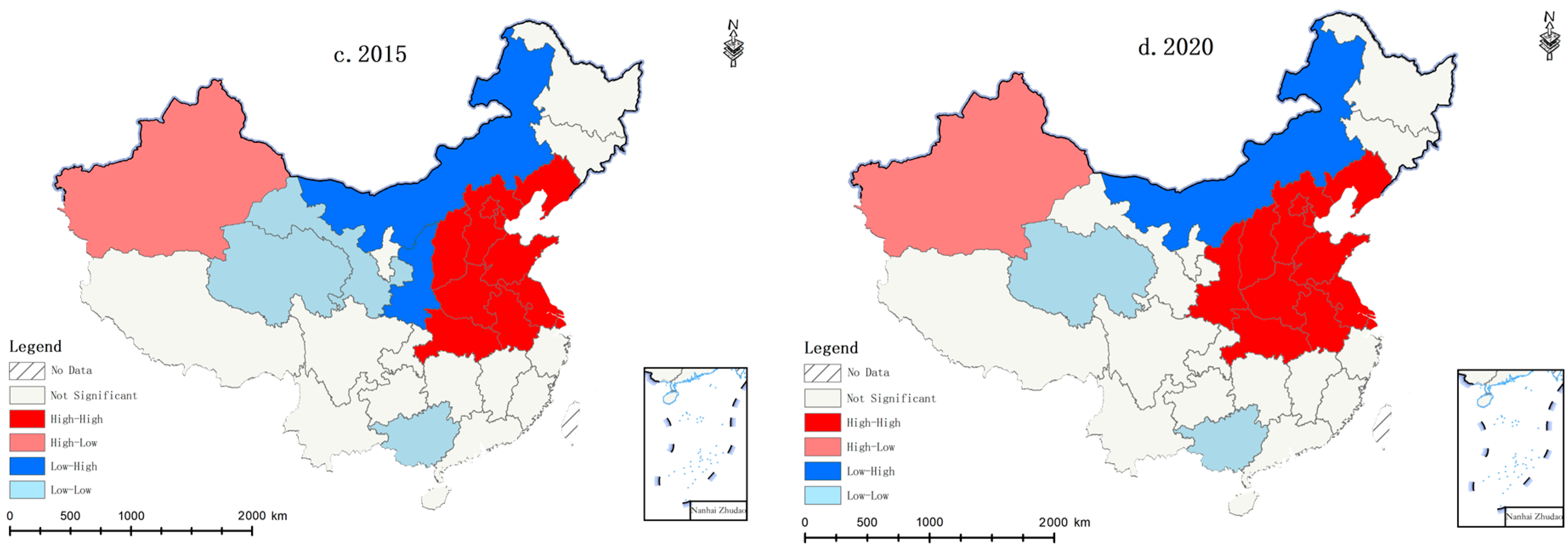
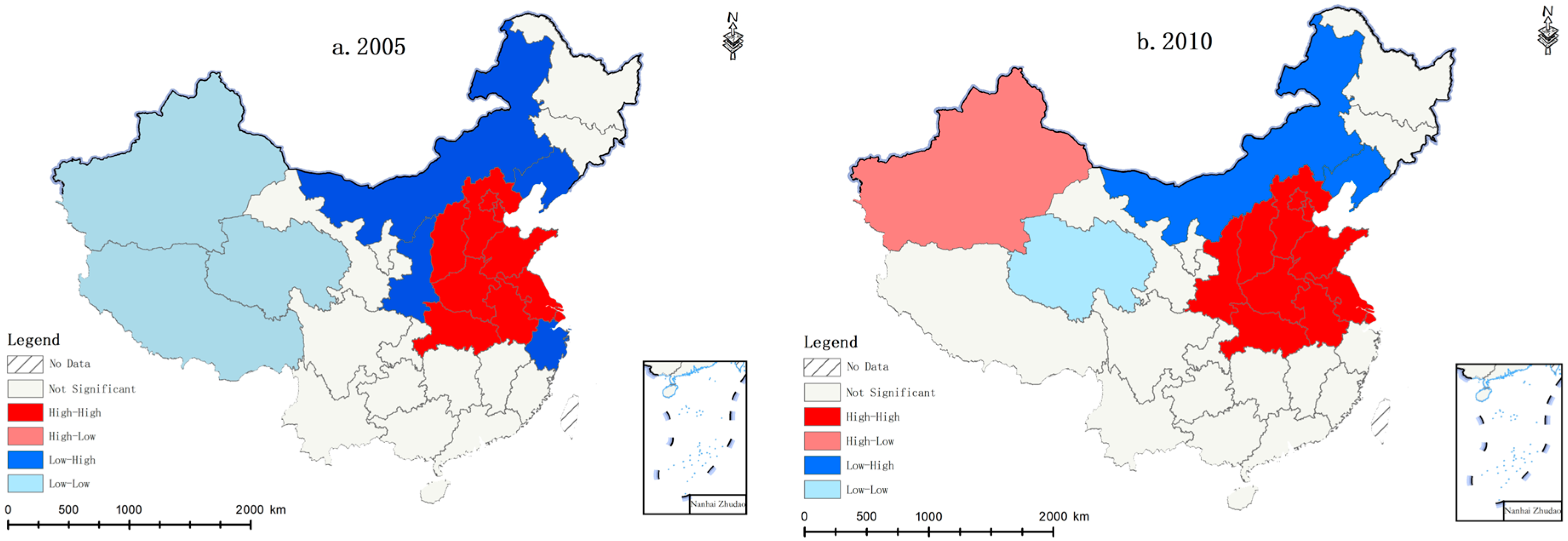
3.1. PM2.5 Spatial Aggregation Characteristics

Figure 1 presents the local Moran indicators of spatial association index (LISA) for PM2.5 concentrations in the years 2005, 2010, 2015, and 2020, demonstrating significant spatial autocorrelation. Notably, regions of high–high agglomeration are predominantly observed in East and North China, whereas both low–low and high–low agglomerations are prevalent in the northwest. These observations highlight the persistent nature of PM2.5 spatial agglomeration throughout the specified period, emphasizing the stable spatial relationships of PM2.5 concentrations across different regions.

3.2. Determination of Spatial Econometric Model

Table 3 presents the detailed model validity test results obtained using 31 spatial inverse distance matrices. The significance levels (P values) are provided in parentheses. Notably, the LM test or robust LM test rejected the null hypothesis at the 5% significance level, indicating that there was spatial autocorrelation between variables [48], so the spatial econometric model could be used for preliminary judgment. The results of the Hausman test all rejected the null hypothesis at the 5% significance level, proving that the model had better results when using fixed effects, so the spatial econometric model used fixed effects. The LR test also rejected the null hypothesis at the 5% significance level, confirming that SDM would not degenerate into SLM and SEM, so SDM was selected in this study.
The panel data constructed for this study had a temporal dimension of 20 years and a cross-sectional dimension covering 31 provincial scale regions, which was a short panel [49]. Therefore, it was challenging to ascertain the presence of autocorrelation within the random disturbance terms associated with reaction time effects. Consequently, these terms were assumed to be independent and identically distributed, and the SDM was employed using individual effects to achieve better results [50]. To confirm the validity of this assumption, the LR test was utilized to compare the model fit of individual fixed effects against dual fixed effects (individual and time). The results indicated that the model employing individual fixed effects demonstrated superior performance compared to the dual fixed effects (Table 4). Accordingly, this study adopted SDM with individual fixed effects.

3.3. Analysis of the Factors Influencing the Spatial Distribution of PM2.5

The direct, indirect, and total effects of 21 independent variable indicators on the dependent variable SDG11.6.2 (concentration of PM2.5) across provincial scale administrative regions in China are shown in Supplementary Figures S1–S21. In the subsequent section, the analysis of the results from the perspectives of both indicators involved and provincial scale regions will be detailed.

3.3.1. Analysis of the Results from the Perspectives of Relevant Indicators Involved

The majority of the results were consistent with the conclusions of previous studies or traditional understanding. For example, the indicators SDG11.7.1 (open space for public use, Figure S16a), SDG15.1.1 (forest area, Figure S19a) and SDG6.6 (water-related ecosystems, Figure S4a) exhibited a synergistic relationship on the direct effect with SDG11.6.2 (concentration of PM2.5) in almost all the regions, suggesting that enhancing the vegetation protection and afforestation can reduce the PM2.5 concentrations for the local areas. The indicators SDG8.1.1 (real GDP per capita growth rate, Figure S8a) and SDG9.1.2 (passenger and freight volume, Figure S9a) exhibited a trade-off relationship on the direct effect with SDG11.6.2 (concentration of PM2.5) in some regions, suggesting that the economic growth and social development of these areas might have negatively impacted on the air quality of these local regions (such as Nei Mongol, Jilin, Hubei, Anhui Sichuan, and Guangxi Province). For SDG6.4.1 (water-use efficiency), some of the regions except Jilin Province exhibited a synergistic relationship on the indirect and total effect (Figure S2b,c) with SDG11.6.2 (concentration of PM2.5), suggesting that improving water use efficiency of local and surrounding areas had contributed to the improvement of air quality for these areas. Similarly, for SDG12.2.1 (material footprint), Beijing and its surrounding areas displayed a synergistic relationship on the indirect and total effect (Figure S17b,c) with SDG11.6.2 (concentration of PM2.5), suggesting that reducing sulfur dioxide emissions of local and surrounding areas had also contributed to the improvement of air quality for these areas.
Additionally, some indicators exhibited varying spatial interrelationships with SDG 11.6.2 (concentration of PM2.5) across different geographical regions. For example, SDG9.1.2 (passenger and freight volume) demonstrated a synergistic effect in both the indirect and overall impact with SDG11.6.2 (concentration of PM2.5) within some southern regions of China, yet manifested a trade-off relationship in some northern regions, including Nei Mongol, Xinjiang, and Tianjin (Figure S9b,c). This divergence may be attributed to the accelerated adoption of new energy vehicles within the passenger and freight sectors in the southern provinces compared to the northern provinces. Such discrepancies could potentially result in a spillover effect, adversely impacting the air quality of the northern regions and their surrounding areas. Therefore, intensifying the promotion of new energy vehicles is essential to realize their potential impact on reducing PM2.5 levels [51]. SDG12.5.1 (national recycling rate) displayed a synergistic effect in both the indirect and overall impact with SDG11.6.2 (concentration of PM2.5) in Sichuan and Nei Mongol, yet manifested a trade-off relationship in Beijing, Tianjin, Hebei, Jiangsu, Henan, and Chongqing (Figure S18b,c). The data used in this study to measure SDG12.5.1 were the comprehensive utilization rates of industrial solid waste, which primarily impacts soil, water, and air quality. This trade-off relationship observed in several economically advanced regions such as Beijing, Tianjin, Jiangsu, Chongqing suggests that the off-site recycling and processing of industrial solid waste can still impact the environmental quality of these areas, owing to spatial spiller over. Enhanced recycling and processing technologies for industrial solid waste are crucial to mitigate further negative impacts. Inappropriate waste disposal methods, such as direct incineration, exacerbate air pollution [52,53]. Table 5 presents the average coefficients of direct, indirect, and total effects of 21 indicators on SDG 11.6.2 (concentration of PM2.5) in all provincial scale regions. From the analysis of average indirect and total effect coefficients, some indicators exhibited significant synergistic effects (an average effect value greater than 1.00), including SDG 15.4 (conservation of mountain ecosystems), SDG 9.4 (sustainable & clean industries), and SDG 6.3 (water quality), and some indicators displayed slightly synergistic effects (an average effect value greater than 0 and less than 1.00), including SDG 6.4.1 (water-use efficiency), SDG6.a (wastewater treatment, recycling, and reuse), SDG7.1.2 (reliance on clean energy), SDG9.1.2 (passenger and freight volume), SDG11.6.1 (municipal solid waste), SDG11.7.1 (open space for public use), SDG12.2.1 (material footprint) and SDG15.1.1 (forest area). Most of these indicators are directly related to the environment, indicating that improvement of natural environment-related indicators can promote the quality of the air environment in the local and surrounding regions. Conversely, indicators showing a trade-off on average indirect and total effect coefficients including SDG6.4.2 (water stress), SDG6.6 (water-related ecosystems), SDG 7.3.1 (energy intensity), SDG 9.2.1 (manufacturing value added), SDG9.b.1 (medium and high-tech industry value added), SDG11.2.1 (convenient access to public transport), SDG 11.3.1 (land consumption), SDG 12.5.1 (national recycling rate), and SDG15.2 (sustainable forests management) are mostly social and economic related indicators. This suggests that the enhancement of socioeconomic-related indicators may, to a certain extent, be achieved at the detriment of air quality in the region and its surrounding areas, an issue that warrants close attention in future development initiatives. Regarding the average direct effect, 11 of the 21 indicators exhibited an insignificant impact on SDG 11.6.2 (concentration of PM2.5) in all provincial-scale regions. The reason for this phenomenon can be attributed to the complexity of the factors influencing PM2.5 concentrations. Despite the potential impact of the 21 indicators selected for this study on PM2.5 concentrations, the variability across different regions—owing to disparities in socioeconomic development and natural resource allocations—necessitates a more granular analysis. This is further compounded by the intricate interplay of regional policy effects, underscoring the need for a broader array of sample sizes. The observational data’s limitations, encompassing a 21-year span from 2000 to 2020 for each region, hinder the ability to conclusively ascertain the influence of each indicator. In contrast, when considering the indirect and total effects, the number of observed indicators escalated to 651, due to the inclusion of elements from neighboring areas, thereby unearthing certain significant correlations.

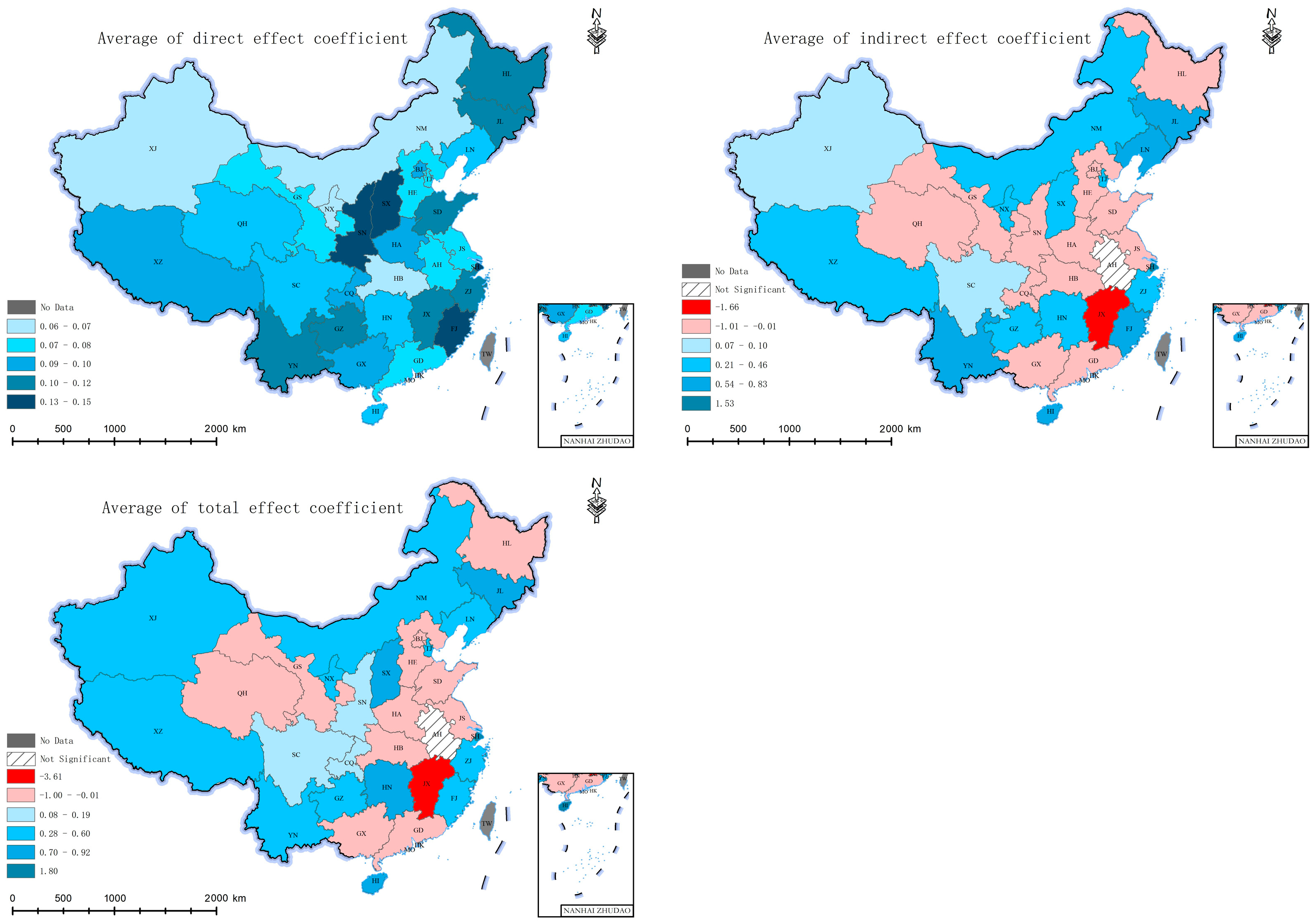
3.3.2. Analysis of the Results from the Provincial-Scale Regions

Table 6 presents the maximal, minimal, and average coefficients of the 21 indicators for their direct, indirect, and total effects on SDG 11.6.2 (concentration of PM2.5) across all provincial-level regions of China. Figure 2 also presents these average values in map form. The results reveal that all 31 observed provincial-scale regions demonstrated a synergistic effect on the average direct effect, which suggests that holistic enhancement of various indicators has had a positive impact on the improvement of PM2.5 in all the local region. This indicates that the policies and measures implemented by the Chinese government have generally played a positive role in reducing PM2.5 levels. Particularly noteworthy is the government’s promulgation in 2011 of the “Weight Method for the Determination of PM10 and PM2.5 in Ambient Air”, marking a significant step forward in environmental regulation. Subsequently, a series of policy documents has been issued to provide guidance to local governments on air quality management. These include the “Technical Specification for the Installation and Acceptance of Continuous Automatic Ambient Air Particulate Matter (PM10 and PM2.5) Monitoring Systems” in 2013, the “Technical Guidance for the Development of Primary Source Emission Inventories of Atmospheric Respirable Particulates (Trial)” in 2014, and the “Technical Requirements and Test Methods for Continuous Monitoring Systems for Flue Gas (SO2, NOX, Particulate Matter) Emissions from Stationary Sources” in 2018. These initiatives demonstrate a comprehensive approach to controlling air pollution and underscore the proactive stance of the Chinese government in enhancing air quality. This aligns with the overarching conclusions drawn from previous research [54,55].
For the indirect and total effects, regions with a larger average of synergy effects included Shanghai, Hainan, Jilin, Hunan, etc. Among these regions, Shanghai has a developed economy and exhibited the largest synergy on the average total effect. The China Statistical Yearbook data showed that tertiary industry’s added value accounted for 73.1% in 2020. Shanghai has significantly enhanced its environmental protection and urban development, following a seven-round, 3-year environmental protection action plan through 2020. The area of green space in Shanghai has expanded from 6561 hectares in 1995 to 171,200 hectares in 2021. Meanwhile, environmental investment soared from RMB 4.65 billion in 1995 to RMB 92.35 billion in 2017. Additionally, there were reductions in smoke emissions and sulfur dioxide exhaust, decreasing from 207.8 thousand tons and 534.1 thousand tons, respectively [56]. Successful industrial transformation has promoted the improvement of air quality. On the other hand, the regions with larger trade-off effects on the average of total effect included Jiangxi, Guangdong, Hebei, Shandong, etc. Most of these are regions with a large proportion of industry and manufacturing. Therefore, while promoting industrial transformation, it is necessary to improve technology and strengthen pollutants, harmless treatment, and secondary utilization [24].
Through the analysis of maximum and minimum indicators related to PM2.5 across 31 province-scale regions in China, it was observed that indicators manifesting maximum values on three or more occasions included SDG6.3 (water quality), SDG6.4.1 (water-use efficiency), SDG6.6 (water-related ecosystems), SDG7.3.1 (energy intensity), SDG9.4 (sustainable and clean industries), SDG15.1.1 (forest area), and SDG15.4 (conservation of mountain ecosystems). Conversely, indicators presenting minimum values more than three times were SDG6.6 (water-related ecosystems), SDG9.2.1 (manufacturing value added), SDG11.2.1 (convenient access to public transport), and SDG15.1.1 (forest area). This highlights the imperative of prioritizing these indicators in the trajectory towards sustainable development.

4. Conclusions and Discussion

This study investigated the spatial autocorrelation and agglomeration characteristics of SDG11.6.2 (concentration of PM2.5) across China from 2000 to 2020, employing spatial econometric models to analyze the influence of various socioeconomic and environmental indicators on PM2.5 distribution. The study’s findings highlight significant spatial autocorrelation in PM2.5 concentrations, with pronounced high–high agglomerations in East and North China, indicating that local governments in this region particularly need to strengthen cooperation to control and prevent air pollution. Using 31 spatial inverse distance matrices for model validation, the study adopted the SDM with individual fixed effects, justified by various model validity tests (LM, robust LM, Hausman, and LR tests) that confirmed the presence of spatial autocorrelation between variables and the superiority of fixed effects in capturing these relationships. The chosen SDM model, applied to panel data encompassing 20 years and 31 provincial regions, effectively addressed the challenges of autocorrelation in the disturbance terms, thereby ensuring model reliability.
In contrast to previous studies, this research systematically analyzed the direct, indirect, and total effects of various influencing factors on PM2.5 at the provincial scale in China. The results reveal the individual influencing factors for each provincial unit, providing auxiliary support for differentiated policymaking in each province. Overall, in all regions with significant results, environmental indicators such as vegetation protection, afforestation, water-use efficiency, and sulfur dioxide emission reduction exhibited synergistic direct effects in lowering PM2.5 levels. Conversely, indicators linked to economic growth and social development, including SDG8.1.1 (real GDP per capita growth rate) and SDG9.1.2 (passenger and freight volume,) showed trade-off direct effects, particularly in regions like Nei Mongol and Jilin, where they correlated with poorer air quality. These regions are primarily characterized by underdeveloped economies, indicating that economic growth in some of China’s less developed provinces still comes at the expense of the environment to a certain extent, without having reached the inflection point of the environmental Kuznets curve.
The study further explored the spatial variance of these effects across provincial-scale regions, revealing a complex phenomenon where some indicators demonstrated synergistic effects in certain regions while exhibiting trade-offs in others. For instance, the adoption of new energy vehicles in southern provinces showed a positive indirect and total effect on air quality improvement, in contrast to northern regions. Similarly, the study identified a trade-off in the comprehensive utilization rate of industrial solid waste in economically advanced areas, suggesting a need for improved recycling and waste processing technologies. Analysis of average coefficients for direct, indirect, and total effects of the indicators underscores the nuanced influence of environmental and socioeconomic factors on SDG11.6.2 (concentration of PM2.5). Some indicators, such as SDG 15.4 (conservation of mountain ecosystems), SDG 9.4 (sustainable and clean industries), and SDG 6.3 (water quality) consistently showed significant positive impacts, advocating for their prioritization in sustainable development efforts. In contrast, certain socioeconomic indicators revealed negative effects, highlighting the critical need for industrial transformation, technological advancement, and effective pollution control measures, especially in industrial-heavy regions. The provincial scale analysis further accentuated the diverse impacts of these indicators across China, with regions like Shanghai showing significant synergies in improving air quality due to successful economic and industrial transformation. On the other hand, provinces with a heavy industrial base face challenges in air quality management, necessitating a balanced approach to industrial growth and environmental sustainability.
However, it is necessary to recognize the potential limitations that may exist in this study. In an effort to quantitatively ascertain the spatial spillover effects of PM2.5, along with its potential influencing factors across a multiplicity of variables and throughout provincial-scale regions in China, this study adopted an iterative approach to refine the conventional inverse distance matrix. This method preserved spatial distance weights between a singular region and its counterparts, thereby generating discrepancies in the outcomes of the direct effect when compared to the indirect and total effects across certain regions and indicators. While such variances might mirror real-world scenarios, they could also stem from biases induced by an inadequate sample size for observation, which was underscored by the pervasive presence of non-significant outcomes in the direct effects observed. Therefore, confirming the reliability of the conclusions derived from this study necessitates further observed data and methodological enhancements for adequate support and verification in the future.

5. Policy Recommendations

The study’s comprehensive analysis illustrates the intricate interplay between environmental policies, socioeconomic development, and air quality. It underscores the importance of a holistic approach to air quality improvement that integrates environmental conservation, economic transformation, and technological innovation. Tailored policies that consider the unique characteristics and needs of each region are imperative for effectively mitigating PM2.5 pollution across China. This nuanced understanding of the factors influencing PM2.5 distribution provides valuable insights for policymakers, suggesting that enhancing air quality necessitates not only environmental measures but also socioeconomic adjustments to foster sustainable development. Based on the study’s findings, here are some policy recommendations to reduce PM2.5 concentrations in China.
  • Enhance inter-regional collaboration: Develop mechanisms for stronger cooperation among local governments, especially in East and North China, to address the high–high agglomerations of PM2.5. This could involve sharing technologies, strategies, and information on successful pollution control measures.
  • Promote environmental conservation measures: Prioritize environmental indicators that have shown synergistic effects in lowering PM2.5 levels, such as vegetation protection, afforestation, water-use efficiency, and sulfur dioxide emission reduction. Implement national and local programs to expand green spaces and urban forests, enhance water conservation practices, and accelerate the shift to cleaner energy sources.
  • Adjust economic and industrial policies: For regions with underdeveloped economies showing a trade-off between economic growth and air quality, policies should encourage industries to adopt cleaner and more sustainable practices. This includes investing in new energy vehicles in the northern provinces, improving the comprehensive utilization rate of industrial solid waste with better recycling and waste processing technologies, and supporting the transition towards sustainable and clean industries.
  • Tailor policies to regional needs and characteristics: Recognize the diverse impact of socioeconomic and environmental indicators across provinces. Implement policies that are customized to the specific needs and challenges of each region, considering their economic, environmental, and social contexts. This may involve differential strategies for regions with heavy industrial bases versus those undergoing economic and industrial transformation.

Supplementary Materials

The following supporting information can be downloaded at: https://www.mdpi.com/article/10.3390/su16083394/s1, Figures S1–S21: Direct effect, indirect effect, and total effect for different explanatory variables on the dependent variable SDG11.6.2 (PM2.5 concentration).

Author Contributions

Conceptualization, Y.C.; methodology, J.L. and Y.C.; formal analysis, Y.C.; data curation, J.L. and Y.C.; writing—original draft preparation, J.L.; writing—review and editing, Y.C. and F.C.; supervision, F.C. All authors have read and agreed to the published version of the manuscript.

Funding

This study was supported by the National Key R&D Program of China (Grant No. 2022YFC3800703), the International Research Centre of Big Data for Sustainable Development Goals (CBAS) [grant numbers CBASYX0906] and the key project of sustainable development international cooperation program by NSFC (Grant No. 42361144883).

Institutional Review Board Statement

Not applicable.

Informed Consent Statement

Not applicable.

Data Availability Statement

The data presented in this study are available on request from the corresponding author.

Conflicts of Interest

The authors declare no conflict of interest.

References

  1. Chen, H.; Zhang, Z.; van Donkelaar, A.; Bai, L.; Martin, R.V.; Lavigne, E.; Kwong, J.C.; Burnett, R.T. Understanding the Joint Impacts of Fine Particulate Matter Concentration and Composition on the Incidence and Mortality of Cardiovascular Disease: A Component-Adjusted Approach. Environ. Sci. Technol. 2020, 54, 4388–4399. [Google Scholar] [CrossRef] [PubMed]
  2. Wilker, E.H.; Osman, M.; Weisskopf, M.G. Ambient air pollution and clinical dementia: Systematic review and meta-analysis. BMJ 2023, 381, e071620. [Google Scholar] [CrossRef] [PubMed]
  3. Requia, W.J.; Adams, M.D.; Arain, A.; Papatheodorou, S.; Koutrakis, P.; Mahmoud, M. Global Association of Air Pollution and Cardiorespiratory Diseases: A Systematic Review, Meta-Analysis, and Investigation of Modifier Variables. Am. J. Public Health 2018, 108, S123–S130. [Google Scholar] [CrossRef] [PubMed]
  4. Wu, W.; Zhang, Y. Effects of particulate matter (PM2.5) and associated acidity on ecosystem functioning: Response of leaf litter breakdown. Environ. Sci. Pollut. Res. Int. 2018, 25, 30720–30727. [Google Scholar] [CrossRef] [PubMed]
  5. Andrei, J.V.; Cristea, D.S.; Nuta, F.M.; Petrea, S.-M.; Nuta, A.C.; Tudor, A.T.; Chivu, L. Exploring the causal relationship between PM 2.5 air pollution and urban areas economic welfare and social-wellbeing: Evidence form 15 European capitals. Sustain. Dev. 2024. early view. [Google Scholar] [CrossRef]
  6. United Nations. Transforming Our World: The 2030 Agenda for Sustainable Development; Department of Economic and Social Affairs Sustainable Development: New York, NY, USA, 2015. [Google Scholar]
  7. Huang, R.-J.; Zhang, Y.; Bozzetti, C.; Ho, K.-F.; Cao, J.-J.; Han, Y.; Daellenbach, K.R.; Slowik, J.G.; Platt, S.M.; Canonaco, F.; et al. High secondary aerosol contribution to particulate pollution during haze events in China. Nature 2014, 514, 218–222. [Google Scholar] [CrossRef] [PubMed]
  8. Chen, Z.; Xie, X.; Cai, J.; Chen, D.; Gao, B.; He, B.; Cheng, N.; Xu, B. Understanding meteorological influences on PM2.5 concentrations across China: A temporal and spatial perspective. Atmos. Chem. Phys. 2018, 18, 5343–5358. [Google Scholar] [CrossRef]
  9. Huang, H.; Jiang, P.; Chen, Y. Analysis of the Social and Economic Factors Influencing PM2.5 Emissions at the City Level in China. Sustainability 2023, 15, 16335. [Google Scholar] [CrossRef]
  10. Ji, X.; Yao, Y.; Long, X. What causes PM2.5 pollution? Cross-economy empirical analysis from socioeconomic perspective. Energy Policy 2018, 119, 458–472. [Google Scholar] [CrossRef]
  11. Yang, D.; Wang, X.; Xu, J.; Xu, C.; Lu, D.; Ye, C.; Wang, Z.; Bai, L. Quantifying the influence of natural and socioeconomic factors and their interactive impact on PM2.5 pollution in China. Environ. Pollut. 2018, 241, 475–483. [Google Scholar] [CrossRef]
  12. Mi, K.; Zhuang, R.; Zhang, Z.; Gao, J.; Pei, Q. Spatiotemporal characteristics of PM2.5 and its associated gas pollutants, a case in China. Sustain. Cities Soc. 2019, 45, 287–295. [Google Scholar] [CrossRef]
  13. Du, Y.; Wan, Q.; Liu, H.; Liu, H.; Kapsar, K.; Peng, J. How does urbanization influence PM2.5 concentrations? Perspective of spillover effect of multi-dimensional urbanization impact. J. Clean. Prod. 2019, 220, 974–983. [Google Scholar] [CrossRef]
  14. Lin, B.; Zhu, J. Changes in urban air quality during urbanization in China. J. Clean. Prod. 2018, 188, 312–321. [Google Scholar] [CrossRef]
  15. Hao, Y.; Liu, Y.-M. The influential factors of urban PM2.5 concentrations in China: A spatial econometric analysis. J. Clean. Prod. 2016, 112, 1443–1453. [Google Scholar] [CrossRef]
  16. Yi, M.; Lu, Y.; Wen, L.; Luo, Y.; Xu, S.; Zhang, T. Whether green technology innovation is conducive to haze emission reduction: Empirical evidence from China. Environ. Sci. Pollut. Res. Int. 2022, 29, 12115–12127. [Google Scholar] [CrossRef] [PubMed]
  17. Lin, Y.; Yang, X.; Li, Y.; Yao, S. The effect of forest on PM2.5 concentrations: A spatial panel approach. For. Policy Econ. 2020, 118, 102261. [Google Scholar] [CrossRef]
  18. Li, J.; Ding, T.; He, W. Socio-economic driving forces of PM2.5 emission in China: A global meta-frontier-production-theoretical decomposition analysis. Environ. Sci. Pollut. Res. 2022, 29, 77565–77579. [Google Scholar] [CrossRef] [PubMed]
  19. Ma, Y.-R.; Ji, Q.; Fan, Y. Spatial linkage analysis of the impact of regional economic activities on PM2.5 pollution in China. J. Clean. Prod. 2016, 139, 1157–1167. [Google Scholar] [CrossRef]
  20. Nuta, F.M.; Nuta, A.C.; Zamfir, C.G.; Petrea, S.-M.; Munteanu, D.; Cristea, D.S. National Carbon Accounting-Analyzing the Impact of Urbanization and Energy-Related Factors upon CO2 Emissions in Central-Eastern European Countries by Using Machine Learning Algorithms and Panel Data Analysis. Energies 2021, 14, 2775. [Google Scholar] [CrossRef]
  21. Ding, Y.; Zhang, M.; Qian, X.; Li, C.; Chen, S.; Wang, W. Using the geographical detector technique to explore the impact of socioeconomic factors on PM2.5 concentrations in China. J. Clean. Prod. 2019, 211, 1480–1490. [Google Scholar] [CrossRef]
  22. Yun, G.; He, Y.; Jiang, Y.; Dou, P.; Dai, S. PM2.5 Spatiotemporal Evolution and Drivers in the Yangtze River Delta between 2005 and 2015. Atmosphere 2019, 10, 55. [Google Scholar] [CrossRef]
  23. Dong, J.; Liu, P.; Song, H.; Yang, D.; Yang, J.; Song, G.; Miao, C.; Zhang, J.; Zhang, L. Effects of anthropogenic precursor emissions and meteorological conditions on PM2.5 concentrations over the “2+26” cities of northern China. Environ. Pollut. 2022, 315, 120392. [Google Scholar] [CrossRef]
  24. Wang, Y.; Duan, X.; Wang, L. Spatial-Temporal Evolution of PM2.5 Concentration and its Socioeconomic Influence Factors in Chinese Cities in 2014–2017. Int. J. Environ. Res. Public Health 2019, 16, 985. [Google Scholar] [CrossRef] [PubMed]
  25. Jin, Y.; Zhang, H.; Shi, H.; Wang, H.; Wei, Z.; Han, Y.; Cong, P. Assessing Spatial Heterogeneity of Factor Interactions on PM2.5 Concentrations in Chinese Cities. Remote Sens. 2021, 13, 5079. [Google Scholar] [CrossRef]
  26. Zhu, M.; Yan, J.; Cheng, X.; Li, F. Investigating the spatiotemporal PM2.5 dynamic and socioeconomic driving forces in beijing based on geographical weighted regression. J. Nonlinear Convex Anal. 2021, 22, 2331–2345. [Google Scholar]
  27. She, Y.; Chen, Q.; Ye, S.; Wang, P.; Wu, B.; Zhang, S. Spatial-temporal heterogeneity and driving factors of PM2.5 in China: A natural and socioeconomic perspective. Front. Public Health 2022, 10, 1051116. [Google Scholar] [CrossRef]
  28. Wei, G.; Sun, P.; Jiang, S.; Shen, Y.; Liu, B.; Zhang, Z.; Ouyang, X. The Driving Influence of Multi-Dimensional Urbanization on PM2.5 Concentrations in Africa: New Evidence from Multi-Source Remote Sensing Data, 2000–2018. Int. J. Environ. Res. Public Health 2021, 18, 9389. [Google Scholar] [CrossRef] [PubMed]
  29. Kong, L.; Tian, G. Assessment of the spatio-temporal pattern of PM2.5 and its driving factors using a land use regression model in Beijing, China. Environ. Monit. Assess. 2020, 192, 95. [Google Scholar] [CrossRef] [PubMed]
  30. Zhang, Y.; Zhou, R.; Hu, D.; Chen, J.; Xu, L. Modelling driving factors of PM2.5 concentrations in port cities of the Yangtze River Delta. Mar. Pollut. Bull. 2022, 184, 114131. [Google Scholar] [CrossRef]
  31. Yan, D.; Ren, X.; Zhang, W.; Li, Y.; Miao, Y. Exploring the real contribution of socioeconomic variation to urban PM(2.5) pollution: New evidence from spatial heteroscedasticity. Sci. Total Environ. 2022, 806, 150929. [Google Scholar] [CrossRef]
  32. Du, Y.; Sun, T.; Peng, J.; Fang, K.; Liu, Y.; Yang, Y.; Wang, Y. Direct and spillover effects of urbanization on PM2.5 concentrations in China’s top three urban agglomerations. J. Clean. Prod. 2018, 190, 72–83. [Google Scholar] [CrossRef]
  33. Nan, Y.; Fan, X.; Bian, Y.; Cai, H.; Li, Q. Impacts of the natural gas infrastructure and consumption on fine particulate matter concentration in China’s prefectural cities: A new perspective from spatial dynamic panel models. J. Clean. Prod. 2019, 239, 117987. [Google Scholar] [CrossRef]
  34. Ledyaeva, S. Spatial econometric analysis of foreign direct investment determinants in Russian regions. World Econ. 2009, 32, 643–666. [Google Scholar] [CrossRef]
  35. Zhang, T.; Zhang, L.; Zhao, D.; Chu, G. Study on the Spatial Spillover Effect of Economic Performance of Public Education Expenditure in China. Educ. Econ. 2021, 3, 20–30. [Google Scholar]
  36. Song, L.; Wan, J. Comparative Research on Interpolation Method of Missing Data. Stat. Decis. 2020, 36, 10–14. [Google Scholar] [CrossRef]
  37. Yang, H.; Zhao, X.; WANG, L. Review of Data Normalization Methods. Comput. Eng. Appl. 2023, 59, 13–22. [Google Scholar] [CrossRef]
  38. Craney, T.A.; Surles, J.G. Model-Dependent Variance Inflation Factor Cutoff Values. Qual. Eng. 2002, 14, 391–403. [Google Scholar] [CrossRef]
  39. Zhang, N.; Yu, K.; Chen, Z. How does urbanization affect carbon dioxide emissions? A cross-country panel data analysis. Energy Policy 2017, 107, 678–687. [Google Scholar] [CrossRef]
  40. Anselin, L. Local Indicators of Spatial Association—LISA. Geogr. Anal. 1995, 27, 93–115. [Google Scholar] [CrossRef]
  41. Sokal, R.R.; Oden, N.L.; Thomson, B.A. Local Spatial Autocorrelation in a Biological Model. Geogr. Anal. 1998, 30, 331–354. [Google Scholar] [CrossRef]
  42. Elhorst, J.P. Dynamic spatial panels: Models, methods, and inferences. J. Geogr. Syst. 2012, 14, 5–28. [Google Scholar] [CrossRef]
  43. LeSage, J.; Pace, R.K. Introduction to Spatial Econometrics; CRC: Boca Raton, FL, USA, 2009. [Google Scholar]
  44. Elhorst, J.P. Applied Spatial Econometrics: Raising the Bar. Spat. Econ. Anal. 2010, 5, 9–28. [Google Scholar] [CrossRef]
  45. Elhorst, J.P. Matlab Software for Spatial Panels. Int. Reg. Sci. Rev. 2014, 37, 389–405. [Google Scholar] [CrossRef]
  46. Lian, Y.-J.; Wang, W.-D.; Ye, R.-C. The Efficiency of Hausman Test Statistics:A Monte-Carlo Investigation. J. Appl. Stat. Manag. 2014, 33, 830–841. [Google Scholar]
  47. Baltagi, B.H. Econometric Analysis of Panel Data; Wiley: Chichester, UK, 2005. [Google Scholar]
  48. Kang, Y.-Q.; Zhao, T.; Yang, Y.-Y. Environmental Kuznets curve for CO2 emissions in China: A spatial panel data approach. Ecol. Indic. 2016, 63, 231–239. [Google Scholar] [CrossRef]
  49. Chen, Q. Advanced Econometrics and Stata Applications; Higher Education Press: Beijing, China, 2010. [Google Scholar]
  50. Ma, L.; Zhang, X. The Spatial Effect of China’s Haze Pollution and the Impact from Economic Change and Energy Structure. China’s Ind. Econ. 2014, 4, 19–31. [Google Scholar]
  51. Su, C.-W.; Yuan, X.; Tao, R.; Umar, M. Can new energy vehicles help to achieve carbon neutrality targets? J. Environ. Manag. 2021, 297, 113348. [Google Scholar] [CrossRef]
  52. Mahato, D.K.; Sankar, T.K.; Ambade, B.; Mohammad, F.; Soleiman, A.A.; Gautam, S. Burning of Municipal Solid Waste: An Invitation for Aerosol Black Carbon and PM2.5 Over Mid-Sized City in India. Aerosol. Sci. Eng. 2023, 7, 341–354. [Google Scholar] [CrossRef]
  53. Nagar, P.K.; Singh, D.; Sharma, M.; Kumar, A.; Aneja, V.P.; George, M.P.; Agarwal, N.; Shukla, S.P. Characterization of PM2.5 in Delhi: Role and impact of secondary aerosol, burning of biomass, and municipal solid waste and crustal matter. Environ. Sci. Pollut. Res. 2017, 24, 25179–25189. [Google Scholar] [CrossRef]
  54. Wu, S.; Yao, J.; Wang, Y.; Zhao, W. Influencing factors of PM2.5 concentration in the typical urban agglomerations in China based on wavelet perspective. Environ. Res. 2023, 237, 116641. [Google Scholar] [CrossRef]
  55. Yang, X.; Wang, J.; Caona, J.; Renna, S.; Ran, Q.; Wu, H. The spatial spillover effect of urban sprawl and fiscal decentralization on air pollution: Evidence from 269 cities in China. Empir. Econ. 2022, 63, 847–875. [Google Scholar] [CrossRef]
  56. Chen, Y.; Bai, Y.; Liu, H.; Alatalo, J.M.; Jiang, B. Temporal variations in ambient air quality indicators in Shanghai municipality, China. Sci. Rep. 2020, 10, 11350. [Google Scholar] [CrossRef] [PubMed]
Figure 1. Local Moran LISA, (a) 2005 (b) 2010 (c) 2015 (d) 2020.
Sustainability 16 03394 g001aSustainability 16 03394 g001b
Figure 2. Average coefficients of the 21 indicators for direct, indirect, and total effects on SDG 11.6.2 (concentration of PM2.5) across all provincial-level regions of China. (AH: Anhui; BJ: Beijing; FJ: Fujian; GS: Gansu; GD: Guangdong; GX: Guangxi; GZ: Guizhou; HI: Hainan; HE: Hebei; HA: Henan; HL: Heilongjiang; HB: Hubei; HN: Hunan; JL: Jilin; JS: Jiangsu; JX: Jiangxi; LN: Liaoning; NM: Nei Mongol; NX: Ningxia; QH: Qinghai; SD: Shandong; SX: Shanxi; SN: Shaanxi; SH: Shanghai; SC: Sichuan; TJ: Tianjing; XZ: Xizang; XJ: Xinjiang; YN: Yunnan; ZJ: Zhejiang; CQ: Chongqing; MO: Macao; HK: Hong Kong; TW: Taiwan).
Sustainability 16 03394 g002
Table 1. Meaning of variables.
VariablesIndicator/
Target
Indicator/Target Short NameIndicator Construction MethodDirection
Explained variableSDG11.6.2Concentration of PM2.5Concentration of PM2.5Negative
Explanatory variablesSDG6.3Water qualityIndustrial water reuse ratePositive
SDG6.4.1Water-use efficiency(total GDP/total water consumption + industrial GDP/industrial water consumption)/2Positive
SDG6.4.2Water stressTotal water consumption/total water resourcesNegative
SDG6.6Water-related ecosystemsNature reserve areaPositive
SDG6.aWastewater treatment, recycling and reuseInvestment in wastewater treatment projectPositive
SDG7.1.2Reliance on clean energyGas penetration ratePositive
SDG7.3.1Energy intensityElectricity consumption per 10,000 yuan of GDPNegative
SDG8.1.1Real GDP per capita growth ratePer capita GDP growth ratePositive
SDG9.1.2Passenger and freight volumeAverage freight volume and passenger volumePositive
SDG9.2.1Manufacturing value addedSecondary industry value added/GDPPositive
SDG9.4Sustainable and clean industriesCarbon dioxide emissionsNegative
SDG9.b.1Medium and high-tech industry value addedTertiary industry value added/GDPPositive
SDG11.2.1Convenient access to public transportNumber of buses per 10,000 peoplePositive
SDG11.3.1Land consumptionUrban built-up area growth rate/population growth rateNegative
SDG11.6.1Municipal solid wastePer capita solid waste generationNegative
SDG11.7.1Open space for public usePer capita park green space areaPositive
SDG12.2.1Material footprintPer capita sulfur dioxide emissionsNegative
SDG12.5.1National recycling rateComprehensive utilization rate of industrial solid wastePositive
SDG15.1.1Forest areaForest coverage ratePositive
SDG15.2Sustainable forests managementArtificial afforestation areaPositive
SDG15.4Conservation of mountain ecosystemsProportion of protected areas to jurisdiction areaPositive
Table 2. Descriptive analysis of variables and VIF of explanatory variables.
VariableSample SizeMeanStdVIF
SDG11.6.265149.0522.8/
SDG6.365171.3129.52.25
SDG6.4.165120.3322.792.34
SDG6.4.265188.220.132.49
SDG6.665111.2420.953.13
SDG6.a65126.3423.982.04
SDG7.1.265172.7127.863.19
SDG7.3.165175.2822.62.67
SDG8.1.165145.9423.931.49
SDG9.1.265138.7925.162.45
SDG9.2.165164.424.555.19
SDG9.465166.9926.953.42
SDG9.b.165129.6221.75.76
SDG11.2.165134.6920.372.6
SDG11.3.165136.5915.871.08
SDG11.6.165181.5721.682.59
SDG11.7.165125.5122.322.94
SDG12.2.165171.3822.623.2
SDG12.5.165161.0224.391.31
SDG15.1.165113.5318.532.15
SDG15.265127.9325.561.64
SDG15.465144.0829.522.54
Table 3. Model validity test results.
TestLM Spatial ErrorRobust LM Spatial ErrorLM Spatial LagRobust LM Spatial LagHausmanLR Test SDM SLMLR Test SDM SEM
Province
Anhui35.592.9753.7821.16−20.33108.95119.55
(0)(0.085)(0)(0)(<0)(0)(0)
Beijing130.15.19129.14.153−38.99179.32185.72
(0)(0.023)(0)(0.042)(<0)(0)(0)
Fujian30.8428.5516.6114.31−40.26205.12178.81
(0)(0)(0)(0)(<0)(0)(0)
Gansu8.670.00211.492.8247.79259.18275.79
(0.003)(0.964)(0.001)(0.093)(0.0012)(0)(0)
Guangdong17.5813.3941.2137.01−23.14169.32152.95
(0)(0)(0)(0)(<0)(0)(0)
Guangxi26.75.55644.9923.85−21.91172.3156.6
(0)(0.018)(0)(0)(<0)(0)(0)
Guizhou30.560.43432.592.466−21.89141.77143.17
(0)(0.51)(0)(0.116)(<0)(0)(0)
Hainan2.09533.2413.4844.6347.02244.74271.82
(0.148)(0)(0)(0)(0.0015)(0)(0)
Hebei61.674.89694.0737.3−12.1575.5473.04
(0)(0.027)(0)(0)(<0)(0)(0)
Henan77.6633.6651.337.327−31.44152.49153.59
(0)(0)(0)(0.007)(<0)(0)(0)
Heilong jiang0.85820.930.51220.58−10.06348347.89
(0.354)(0)(0)(0)(<0)(0)(0)
Hubei49.290.00258.28.912−17.71134.09127.02
(0)(0.967)(0)(0.003)(<0)(0)(0)
Hunan25.787.51249.3931.12−23.9147.37137.21
(0)(0.006)(0)(0)(<0)(0)(0)
Jilin1.13546.7725.0170.65−26.48211.54306.08
(0.287)(0)(0)(0)(<0)(0)(0)
Jiangsu38.1210.2366.8138.91−18.8134.71158.67
(0)(0.001)(0)(0)(<0)(0)(0)
Jiangxi13.956.8145.2388.14−95.63139.38125.57
(0)(0)(0)(0)(<0)(0)(0)
Liaoning6.81822.3330.5746.08−13.16212.74262.84
(0.009)(0)(0)(0)(<0)(0)(0)
Nei Mongol3.3432.432.26131.35−127327.52400.1
(0.068)(0)(0)(0)(<0)(0)(0)
Ningxia3.4129.9710.9317.48139.2348.65354.94
(0.065)(0.002)(0.001)(0)(0)(0)(0)
Qinghai0.2535.6561.2336.635−115.8399.63297.6
(0.615)(0.017)(0.267)(0.01)(<0)(0)(0)
Shandong48.250.38563.5715.71−14.32181.13185.45
(0)(0.535)(0)(0)(<0)(0)(0)
Shanxi7.79413.3426.9432.49−25.56266.21241.61
(0.005)(0)(0)(0)(<0)(0)(0)
Shaanxi3.2626.53813.1116.38−19.79260.29298.36
(0.071)(0.011)(0)(0)(<0)(0)(0)
Shanghai61.192.26959.810.889−3.69281.47274.72
(0)(0.132)(0)(0.346)(<0)(0)(0)
Sichuan3.1665.58511.2413.66−23.54220.31236.99
(0.075)(0.018)(0.001)(0)(<0)(0)(0)
Tianjing22.555.72847.9631.14−6.8119.37129.15
(0)(0.017)(0)(0)(<0)(0)(0)
Xizang0.0460.2580.0020.214−229.9461.58403.97
(0.029)(0.611)(0.063)(0.644)(<0)(0)(0)
Xinjiang2.28923.060.89121.6641.68357.28337.12
(0.13)(0)(0)(0)(0.00680)(0)(0)
Yunnan27.6631.579.41813.332.93275.63286.55
(0)(0)(0)(0)(1)(0)(0)
Zhejiang47.910.19449.531.812−45.64130.13125.76
(0)(0.66)(0)(0.178)(<0)(0)(0)
Chongqing28.189.98453.1934.99−21.85172.61147.2
(0)(0.002)(0)(0)(<0)(0)(0)
Note: The p value is in parentheses.
Table 4. Model goodness of fit for individual and dual fixed effects.
ProvinceIndBoth
Anhui0.66790.0068
Beijing0.7036\
Fujian0.68490.0537
Gansu0.69580.0276
Guangdong0.68680.1608
Guangxi0.69250.0071
Guizhou0.69420.0508
Hainan0.62090.1727
Hebei0.69050.3943
Henan0.66950.0162
Heilong jiang0.67720.1642
Hubei0.68190.3182
Hunan0.69630.1046
Jilin0.56960.021
Jiangsu0.69180.0856
Jiangxi0.6850.0357
Liaoning0.68350.3069
Nei Mongol0.68360.0225
Ningxia0.69910.1531
Qinghai0.69910.0012
Shandong0.69720.4073
Shanxi0.68570.2835
Shaanxi0.69740.1732
Shanghai0.694\
Sichuan0.69660.03
Tianjing0.68450.3102
Xizang0.7141\
Xinjiang0.69440.2579
Yunnan0.69870.0002
Zhejiang0.68660.15
Chongqing0.69440.0034
Note: \ indicates that the model has no goodness of fit.
Table 5. Average coefficients of direct, indirect, and total effects of 21 indicators on SDG 11.6.2 (concentration of PM2.5) in all provincial-scale regions.
IndicatorAverage of Direct EffectAverage of Indirect EffectAverage of Total Effect
SDG6.3−0.0731 1.08921.0800
SDG6.4.1\0.98630.8947
SDG6.4.2\−0.6270−0.6630
SDG6.60.3213−5.3188−4.2059
SDG6.a\0.13960.1403
SDG7.1.2\0.16070.0918
SDG7.3.10.0858−0.2974−0.1009
SDG8.1.1−0.03380.0463−0.0306
SDG9.1.2−0.04190.19260.1813
SDG9.2.10.1119−0.9859−0.8227
SDG9.4\1.33281.4353
SDG9.b.10.1338 −0.2971−0.1134
SDG11.2.1\−0.5387−0.5223
SDG11.3.1\0.16550.1705
SDG11.6.1\0.68280.8798
SDG11.7.10.0922 −0.02900.2980
SDG12.2.1\0.43580.7830
SDG12.5.1\−0.5060−0.5488
SDG15.1.10.2703 0.08700.6032
SDG15.2\−0.1080−0.0715
SDG15.4−0.26303.53403.3798
Note: \ means the result is not significant.
Table 6. The maximal, minimal, and average coefficients of the 21 indicators for their direct, indirect, and total effects on SDG 11.6.2 (concentration of PM2.5) across all provincial-level regions of China.
ProvinceMaximumMinimumAverage
IndicatorValueEffect TypeIndicatorValueEffect TypeDirect EffectIndirect EffectTotal Effect
AnhuiSDG15.1.10.29DirectSDG6.3−0.0669Direct 0.0707 //
BeijingSDG12.2.11.328Total SDG7.3.1−2.647Indirect 0.0910 −0.2538−0.1874
FujianSDG6.4.11.312Total SDG9.2.1−1.03Indirect 0.1304 0.54300.5670
GansuSDG6.4.10.71Indirect SDG9.2.1−1.209Indirect 0.0767 −0.0989−0.0974
GuangdongSDG15.1.10.264DirectSDG11.6.1−1.623Indirect 0.0727 −1.0108−1.0018
GuangxiSDG11.6.11.715Total SDG6.4.2−3.292Indirect 0.0937 −0.4343−0.4075
GuizhouSDG9.42.235Indirect SDG9.2.1−0.769Indirect 0.1061 0.30040.3190
HainanSDG9.42.365Total SDG15.1.1−1.66Indirect 0.0806 0.77840.9211
HebeiSDG15.48.056Indirect SDG6.6−10.63Indirect 0.0714 −0.6027−0.6017
HenanSDG15.412.4Indirect SDG6.6−15.29Indirect 0.0912 −0.2632−0.2365
HeilongjiangSDG6.4.11.182Indirect SDG7.3.1−1.866Indirect 0.1111 −0.4598−0.5265
HubeiSDG11.6.12.146Total SDG6.3−1.936Total 0.0611 −0.0138−0.0194
HunanSDG9.42.633Total SDG15.1.1−1.115Indirect 0.0784 0.20582.6330
JilinSDG6.68.23Total SDG6.4.2−2.43Total 0.1114 0.83400.9050
JiangsuSDG15.43.477IndirectSDG12.5.1−0.573Indirect 0.0757 0.54610.1183
JiangxiSDG6.60.351DirectSDG15.4−3.551Total 0.1140 −1.6323−3.5510
LiaoningSDG6.32.166Indirect SDG11.2.1−0.85Indirect 0.0836 0.61000.6020
Nei mongolSDG15.1.12.932Total SDG9.b.1−0.788Total 0.0573 0.43500.5924
NingxiaSDG7.3.10.654Total SDG15.2−0.249Direct 0.0646 0.23220.3098
QinghaiSDG6.61.248Total SDG15.1.1−2.026Indirect 0.0799 −0.6404−0.5391
ShandongSDG6.35.409Indirect SDG6.6−11.28Indirect 0.1233 −0.6105−0.5888
ShanxiSDG9.41.903Total SDG9.2.1−0.774Indirect 0.1509 0.45830.7027
ShaanxiSDG7.3.10.939Total SDG15.1.1−1.198Indirect 0.1302 −0.04750.1953
ShanghaiSDG6.37.424Indirect SDG11.2.1−0.174Indirect 0.1457 1.52971.7957
SichuanSDG7.3.11.5Total SDG9.2.1−1.227Indirect 0.0838 0.13750.1884
TianjingSDG6.31.568Indirect SDG6.4.1−0.304Total 0.0714 0.34260.3526
XizangSDG15.44.412Indirect SDG6.6−3.52Indirect 0.0942 0.19340.2478
XinjiangSDG9.41.142Indirect SDG9.b.1−0.471Indirect 0.0651 0.04130.3476
YunnanSDG9.41.42Indirect SDG11.2.1−0.942Indirect 0.1043 0.55680.4674
ZhejiangSDG6.4.10.873Indirect SDG11.7.1−0.476Indirect 0.1115 0.30980.5063
ChongqingSDG6.4.10.913Indirect SDG12.5.1−0.664Indirect 0.0995 −0.09800.1285
Disclaimer/Publisher’s Note: The statements, opinions and data contained in all publications are solely those of the individual author(s) and contributor(s) and not of MDPI and/or the editor(s). MDPI and/or the editor(s) disclaim responsibility for any injury to people or property resulting from any ideas, methods, instructions or products referred to in the content.

