Abstract
As a new urban model, the 15-min city has gradually become a touchstone with which to measure the future sustainability of cities. With a time-limited planning of urban living circles, urban residents can be allowed to access basic daily needs, such as food, health and education, while walking or cycling, thus reducing motor traffic and carbon dioxide emissions and contributing to the improvement of people’s well-being and the environmental climate. Within the temporal and spatial confines of the 15-min living sphere, governmental authorities and community bodies commonly integrate public art installations into public spaces to enrich spatial dynamics, cultivate cultural identities, enhance environmental aesthetics, elevate service quality, and foster communal interactions. This study aims to probe into the impact of public art on encouraging urban pedestrianism within the specific context of the 15-min community living sphere along the Suzhou River in northern Shanghai. Drawing upon Stimulus–Organism–Response (SOR) theory, a theoretical framework is constructed to unravel the mechanisms by which public art influences residents’ propensity for walking, encompassing the attributes of public art, perceived value, and walking intention. Employing Confirmatory Factor Analysis (CFA), the model is analyzed to scrutinize the proposed hypotheses. Through this research, we establish and substantiate a novel and pertinent theoretical perspective for advancing human-centric and sustainable urban regeneration. The findings underscore that integrating public art within the framework of constructing 15-min community living spheres contributes to catalyzing proactive urban pedestrianism by enhancing its value proposition.
1. Introduction
With the continuous advancement of urbanization, it is projected that by 2025 over 70% of the global population will reside in cities [1]. The significant concentration of populations in urban areas poses multifaceted challenges in areas such as transportation, sustainability, and energy. Consequently, urban planners are increasingly alerted to the inadequacy of the traditional “car-centric” approach to transportation planning for future urban development scenarios. Against this backdrop, the concept of “Living Circles” has been introduced. This concept delineates the spatial scope required for daily activities, such as work, shopping, leisure, education, and healthcare, around residents’ places of residence, defining this scope as the fundamental spatial unit of living circles. Emphasizing proximity in providing all essential services to reduce reliance on automobiles, it advocates for the establishment of green transportation networks primarily focused on walking or cycling, thereby promoting the sustainable development of urban ecology [2]. Currently, cities such as Shanghai, Paris, Melbourne, and Ottawa have initiated “temporal urbanism” planning practices to actively address urban challenges. In 2016, Shanghai proposed the strategy of constructing 15-min Community Living Circles (CLC) in its development blueprint for 2017–2035 [3], subsequently releasing guidelines and standards, such as the Shanghai 15-Minute Community Living Circle Planning Guide [4], Spatial Planning Guidelines, and Community Living Units. The goal is to create a space environment that is conducive to living, working, leisure, aging, and learning, as well as to establishing a sustainable community life. To achieve this, Shanghai has gradually embarked on progressive and incremental urban renewal practices in recent years.
As early as the 1960s, public art emerged as a cultural tool for addressing urban issues in many countries, gradually forming a comprehensive interdisciplinary field that incorporates contributions from disciplines such as architecture, landscape architecture, urban design, and art history [5]. Presently, the definition of public art is diverse, encompassing not only specific art pieces or activities but also permeating various aspects of public life, enriching public spaces for the community. In September 2021, Shanghai organized the third Urban Space Art Season under the theme of “15-Minute Community Living Circles—People’s City”. This event utilized 21 communities as exhibition venues, placing various types of public art at key locations within these communities. Citizens were invited to explore, experience, and participate in community building and public art activities, showcasing the integration of urban spaces and art. Against the backdrop of constructing 15-min CLCs, public art serves as a cultural tool that connects the public in the construction of public domains. It enhances people’s experiences of urban environments, stimulates spatial production, and fosters cultural identity and community solidarity. To a certain extent, it represents the demands of public interests, engaging stakeholders in collaborative models and attracting broad public participation, thus exploring possibilities for creating more effective and sustainable cultural communities.
According to surveys, individuals’ choice of walking in urban settings tends to align with their immediate interests [6]. It has been observed that, in most cases, community residents choose their mode of transportation based on the distance between their origin and destination [7]. Within a certain spatial range, if walking is feasible, people’s willingness to walk significantly increases [8,9]. However, beyond a certain spatial threshold, coupled with considerations of transportation routes, the propensity for walking decreases. Given the current achievements in the construction of 15-min CLCs, the convenience of daily travel for individuals has been increasingly enhanced. Governments are placing greater emphasis on the development of green transportation networks during urban renewal processes. Against this backdrop, the question arises: can the installation of public art, aimed at environmental improvement, cultural shaping, service improvement and public interaction, enhance the appeal of urban spaces and promote pedestrian activity?
Exploring this perspective can assist urban decision makers in taking targeted measures by setting up relevant public art projects based on people’s needs, encouraging public participation, enhancing spatial attractiveness, and thus promoting walking choices. However, existing literature on addressing this issue through public art has certain limitations. Firstly, most studies focus on public art itself, neglecting its perspective as a public service. Secondly, theoretical studies suggest that public art influences people’s willingness to engage in interaction, but there is a lack of actual sample studies, particularly quantitative research. Thirdly, existing research mainly concentrates on the macro-level impacts of public art on urban culture, economy, and ecology, but pays little attention to the specific interactive relationships between public art and individuals at the micro-level.
Therefore, this study poses the research question: can public art within the 15-min CLC in Shanghai promote people’s active choices regarding urban walking? We adopt a case study analysis as the primary research method, selecting the area along the north Suzhou River in Jing’an District, Shanghai, as the research area and focusing on the public art projects within this scope. The research framework of this paper is based on Stimulus–Organism–Response (SOR) theory and employs quantitative research structured into five main sections. The first part provides a brief overview of relevant factors and literature reviews regarding how public art influences people’s choices of urban walking within the context of constructing 15-min CLCs. The second part examines the research question through a literature review, surveys, and web data, proposing the research model and hypothesis propositions. The third part describes the case study area, research methods, and data collection procedures. The fourth part employs CFA structural equation modeling to examine 346 questionnaires collected from residents in the area, of which 315 were valid. The final section discusses the positive impacts and practical significance of public art installations within the 15-min CLC on people’s choices regarding urban walking, reflects on the limitations of the study, and suggests future research directions.
2. Literature Review
2.1. 15-Min CLCs
At present, urban development is facing multiple challenges caused by climate change and social ecology. In this context, reconsidering the sustainable urban development model and urban transformation has been regarded as the future direction and inevitable choice of global urban development [10]. As early as the 1950s and 1960s, Japan put forward the concept of the “life circle” in a broad sense for the first time in response to urban problems such as resource concentration, regional differences and environmental pollution [11]. The concept defines the space scope of work, shopping, leisure, education and medical care required for daily life based on residence, and defines this scope as the basic space unit of the life circle. Subsequently, South Korea and Taiwan (China) in Asia have also carried out research and practice concerning the concept of the life circle. In the 1980s, North America witnessed the emergence of the New Urbanism planning movement, which prioritized livable spaces as a fundamental principle. This movement advocated for locating commercial and municipal centers within walking distance of the majority of households and emphasized the integration of public spaces with community life [12]. Urban planners gradually recognized the necessity for a more sustainable transportation model to replace automobile-dominated urban sprawl.
At the Paris Climate Summit in 2016, Carlos Moreno first put forward the concept of a 15-min city based on “chrono-urbanism” [13]. This concept emphasizes the proximity of all basic services to break the dependence on cars, thus promoting ecological sustainability, social interaction and public participation [14]. In the same year, Shanghai formulated planning guidelines for the construction of the “15-min CLC” and proposed the community as the platform for urban basic life. The goal is to build Shanghai into a sustainable, safe, friendly and comfortable smart city. Residents can meet their needs for education, culture, medical care, elderly care, sports, commerce and other public service facilities within a 15-min walking range. From the perspective of radiation scope, these all radiate outward from the center, emphasizing the accessibility of space within the time limit, whether using the concept of the life circle proposed by Japan in the early years, the 15-min city proposed by Carlos Moreno, or the 15-min CLC plan implemented in Shanghai. Due to the ongoing renewal of, and transition phases in, urban environments and infrastructure development, there are evident shortcomings when looking at the current status and the set goals of community convenience. Therefore, within this context, urban planning does not solely consider the perspective of people’s choices of urban walking. This paper adopts a more nuanced approach by selecting public art that combines public accessibility and artistic qualities within the living circle range as a medium. Specifically, it explores the impact of community spaces on people’s behavior, aiming to complement the research into and practice of future 15-min city visions.
2.2. Public Art
Influenced by 19th-century architectural beautification policies, early forms of public art predominantly consisted of murals, sculptures, and architectural embellishments [15]. In 1959, Philadelphia passed the first Percent for Art [16] legislation in the United States, mandating a fixed percentage of building budgets for the creation of art in conjunction with architectural and public space enhancement, aiming to strengthen urban character and enhance public welfare [17]. By the 1970s and 1980s, Western countries had entered a period of de-urbanization transition, gradually undergoing structural adjustments in urban industries, with the tertiary sector. focusing on tourism, services, and knowledge. experiencing rapid growth. Urban spaces urgently required the infusion of cultural vitality and improvement of spatial quality. Subsequently, numerous cities in the United States, such as Seattle, Chicago, New York, Los Angeles and Washington, began implementing public art programs, making it a consensus to shape the city’s cultural brand and gradually diversify its development path [18]. The scope of public art expanded to include architectural decoration, lighting art, plaza sculptures, public facilities, and artistic events. In 1991, American artist Suzanne Lacy introduced the concept of a new type of public art oriented toward public issues, involving public participation, interaction, and collaboration, broadening the scope of public art to encompass tangible and intangible, permanent and temporary forms [19]. The extension of the public art category allowed more cities to see its potential in boosting urban cultural development. In 1994, Australia’s Creative Nation [20] policy declared, “Cultural policy is economic policy, culture creates wealth”. That same year, the City of Sydney introduced the Public Art Policy, aiming to transform Sydney into a vibrant city characterized by a ubiquitous artistic and cultural presence, thereby stimulating urban vitality [21]. The concept of activating urban spaces through cultural development via public art has been continuously validated through concrete, practical endeavors, affirming its value in the process.
Streets and public spaces are crucial sites for individuals to experience urban environments and culture, regarded as having “clear social purposes, aimed at encouraging pedestrian activity to strengthen community connections and promote a sense of place” [22]. However, empirical research supporting the notion that the installation of public art in streets and public spaces can support pedestrian activity has yet to be confirmed by social science studies. While observing pedestrian activity, Kellerman pointed out that “whether walking on the street, interacting with space or companions, encourages or inhibits any form of social contact has always been questionable” [23]. The main reason for this uncertainty lies in the diversity and complexity of influencing factors, making it difficult to attribute the encouragement of pedestrian behavior solely to public art’s influence on urban environments, community awareness, or neighborhood attachment. Therefore, this paper aims to delve into specific case studies to explore whether public art, as an artistic medium, can inject vitality into spaces and attract public participation by improving spatial environments, enhancing community services, and perpetuating cultural genes. This exploration seeks to encourage urban walking by revitalizing spaces and engaging the public.
2.3. City Walk
In the field of urban planning and design, the concept of walkable cities has garnered widespread acknowledgment and application by academia and governmental planning departments alike, aiming to achieve the goals of sustainable urban development. From Ebenezer Howard’s conception of “Garden Cities” [24] in the late 19th century to Le Corbusier’s vision of “Modern Cities” [25] and from Clarence Perry’s formulation of the Neighborhood Unit theory in 1929 to the emergence of the New Urbanism planning movements in the postmodern era, all these theories and movements share a common belief that cities should be conducive to walking. Some scholars emphasize the dual nature of walkable cities, delineating physical elements (streets, spaces, proximity, and convenience) and perceptual elements (comfort, safety, enjoyment) [26,27,28], thus affirming that urban walking encompasses purposeful transportation, leisure, recreation and social interaction. Numerous studies have classified different walking behaviors based on varying purposes. Among the most classic is Gehl’s categorization of outdoor activities into three types: necessity activities, spontaneous activities, and social activities [29]. Gehl also proposes how cities can be planned in a more human-centric manner, considering “walkability” and “transforming public life through public spaces” as goals of urban planning.
2.4. The Stimulus–Organism–Response (S–O–R) Theory
The Stimulus–Organism–Response (S–O–R) theory primarily stems from the Stimulus–Response (S–R) theory [30]. The S–R theory posits that individual behavioral responses are outcomes influenced by external stimuli. However, the S–R theory does not account for the impact of external stimuli on internal consciousness and psychological activities [31]. Recognizing this limitation, psychologist Woodworth first introduced the SOR model in 1926 [32]. Woodworth proposed that stimuli from the external environment influence human emotional consciousness, subsequently affecting individual behavioral responses. Therefore, responses to external stimuli are not mechanical and passive; organisms can process external stimuli and generate behavioral responses that reflect individual will. The SOR model has been widely applied in cognitive and developmental psychology, behaviorism, and other fields, covering various behaviors. such as cognitive responses, behavioral choices, participation, and consumption reviews. To study someone’s behavioral responses, we must explore the effects of different stimuli on the organism’s cognitive and emotional consciousness [33]. Thus, employing the SOR model is applicable for empirically verifying the impact of public art within a 15-min accessible spatial range on people’s choices regarding urban walking.
3. Research Framework and Hypothesis
3.1. Theoretical Framework and Variables
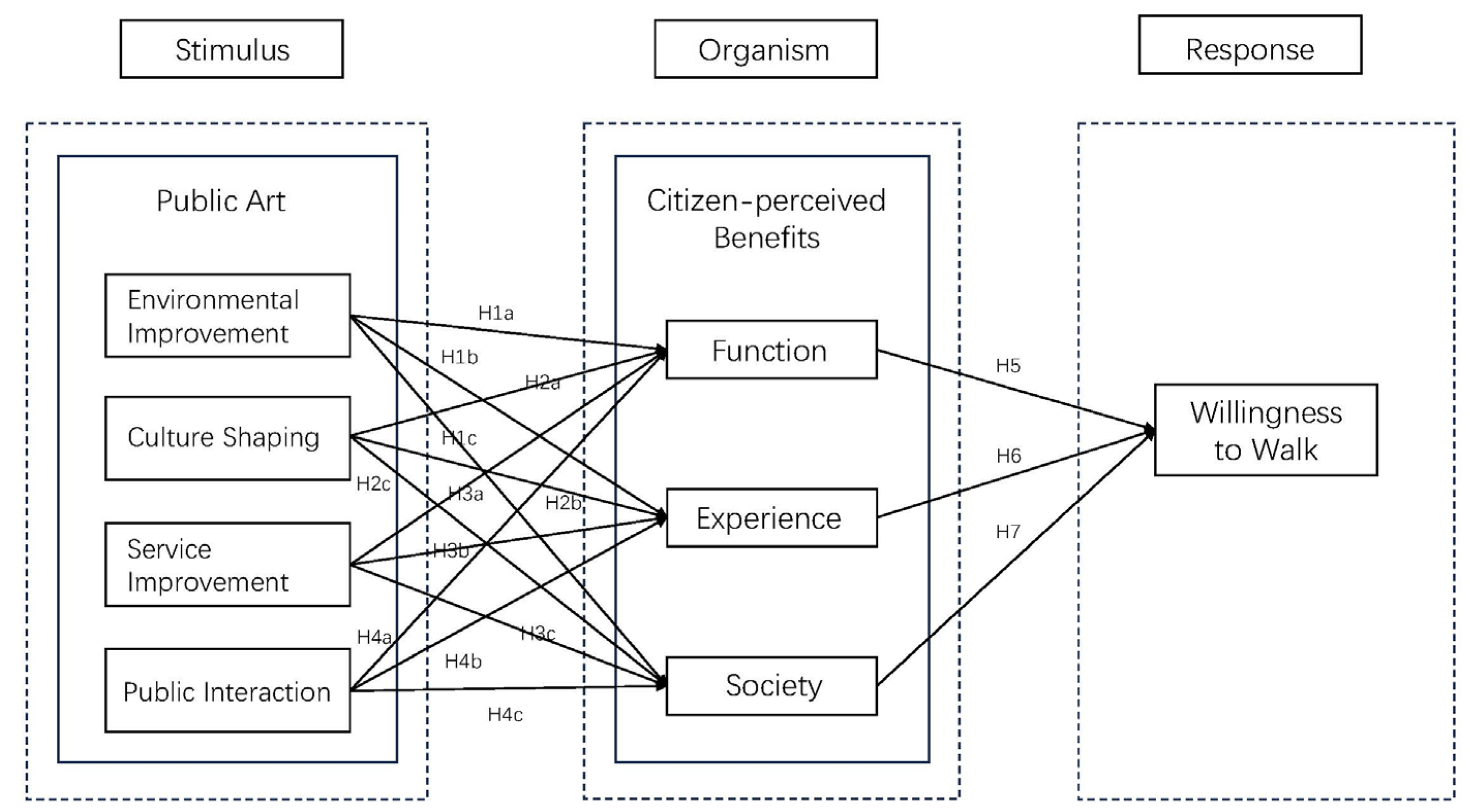
The research framework of this study is based on the Stimulus–Organism–Response (SOR) theory (see Figure 1), which posits the existence of external stimuli that elicit behavioral responses involving either approach or avoidance, influenced by the organism’s internal psychological processes. To investigate an individual’s behavioral responses, it is imperative to explore how different stimuli affect cognitive and emotional states [34]. The research model integrates discussions on the value theory of public art and field surveys conducted in the 15-min CLC in Shanghai. Building upon this foundation, the SOR model is utilized to empirically examine the impact of public art on urban walking within these living circles. The evaluation is based on the influence of public art on the environment, focusing primarily on four dimensions: environmental improvement, cultural shaping, service enhancement, and public interaction. These four dimensions are studied as independent variables to assess the influence of public art on individuals’ willingness to engage in walking, with residents’ perceptions of the functional, experiential, and social values of walking routes serving as mediators.
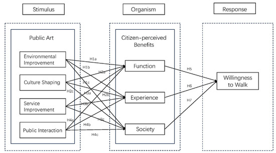
Figure 1.
Proposed research model diagram (arrows indicate positive relationships. H1a: The arrow from Environmental Improvement to Function indicates that environmental improvement has a positive and significant impact on urban function).
In this study, we have distilled four main aspects of the impact of public art on the environment: environmental improvement, cultural shaping, service enhancement, and public participation. These four primary aspects are widely regarded as encompassing the functional characteristics of public art [35], as evidenced in numerous literature sources. Therefore, they are considered as the four independent variables. Perceived benefits refer to individuals’ perceptions of the positive consequences of their specific behaviors [36]. Citizen-perceived benefits are distinguished by three dimensions: functional value, experiential value, and social value. These dimensions stem from preliminary research and literature review findings, indicating that people’s perceptions of environmental space and travel provide not only spatial experience and functional services but also significant social and psychological benefits [37], such as perceived social interaction and ecological benefits. Thus, this study considers the three dimensions of citizen perceived value as mediating variables between public art and people’s willingness to walk. Walking willingness refers to people’s preference for walking as a mode of transportation within a certain spatio-temporal range, which is often influenced by various factors. For example, high-quality sidewalks have a positive impact on walking willingness [38], and the spatio-temporal range of destinations affects walking willingness. Given that the study sets walking willingness within a 15-min spatial range and focuses on the influence of walking environment, it is reasonable to expect that walking willingness will be influenced by public art and citizens’ perceived benefits.
3.2. Hypothetical Proposition
The installation of public art in a space contributes to the enhancement of its public and artistic aspects [39], thus influencing the overall spatial environment. Firstly, from a material perspective, the placement of public art aids in improving the spatial environment, exemplified by the beautification effect of landscapes, murals, and sculptures. Secondly, from a cultural standpoint, public art can play a significant role in cultural-led urban revitalization, cultural shaping, and fostering diverse and inclusive communities [40]. Thirdly, from a functional service perspective, composite public art facilities can provide residents and tourists with amenities, such as rest areas, wayfinding, and a range of public service functions. Lastly, from a social perspective, strengthening public interaction and participation has positive effects on social cohesion and the development of democratic cities [41]. Theoretically, it is believed that environmental improvement, cultural shaping, service enhancement, and public participation have varying degrees of influence on citizens perceived benefits, primarily manifested in the dimensions of functional value, experiential value, and social value.
Therefore, we hypothesized the following:
- Hypothesis 1a (H1a). Environmental improvement has a positive and significant influence on Function.
- Hypothesis 1b (H1b). Environmental improvement has a positive and significant influence on Experience.
- Hypothesis 1c (H1c). Environmental improvement has a positive and significant influence on Society.
- Hypothesis 2a (H2a). Cultural shaping has a positive and significant influence on Function.
- Hypothesis 2b (H2b). Cultural shaping has a positive and significant influence on Experience.
- Hypothesis 2c (H2c). Cultural shaping has a positive and significant influence on Society.
- Hypothesis 3a (H3a). Service improvement has a positive and significant influence on Function.
- Hypothesis 3b (H3b). Service improvement has a positive and significant influence on Experience.
- Hypothesis 3c (H3c). Service improvement has a positive and significant influence on Society.
- Hypothesis 4a (H4a). Public interaction has a positive and significant influence on Function.
- Hypothesis 4b (H4b). Public interaction has a positive and significant influence on Experience.
- Hypothesis 4c (H4c). Public interaction has a positive and significant influence on Society.
Within the 15-min walkable neighborhood radius, theoretically, we posit that citizen-perceived benefits are significantly associated with the functionality of services, the convenience of travel experiences, and the effectiveness of social interactions. Functional deficiencies and poor pedestrian experiences may influence citizens perceived benefits and diminish people’s willingness to walk. It is anticipated that citizens’ perceptions of the functional, experiential, and social values of the pedestrian environment serve as mediators between public art and walking intentions.
Therefore, we hypothesized the following:
- Hypothesis 5 (H5). The function has a positive and significant influence on Willingness to walk.
- Hypothesis 6 (H6). Experience has a positive and significant influence on Willingness to walk.
- Hypothesis 7 (H7). Society has a positive and significant influence on Willingness to walk.
4. Research Case and Methods
4.1. Case Study: North Suzhou River Community in Shanghai
Shanghai stands for China as the pioneer and fastest-growing, most mature city in advocating city walks. Since 2018, the Shanghai Municipal Administration of Culture and Tourism has introduced multiple city walk routes and organized various activities to encourage both residents and tourists to stroll through the city. Additionally, in conjunction with the construction of the 15-min CLC and urban spatial art activities in Shanghai, this study selects the North Suzhou River community in the Jing’an District, which represents the waterfront spaces as the most significant research area for investigation.
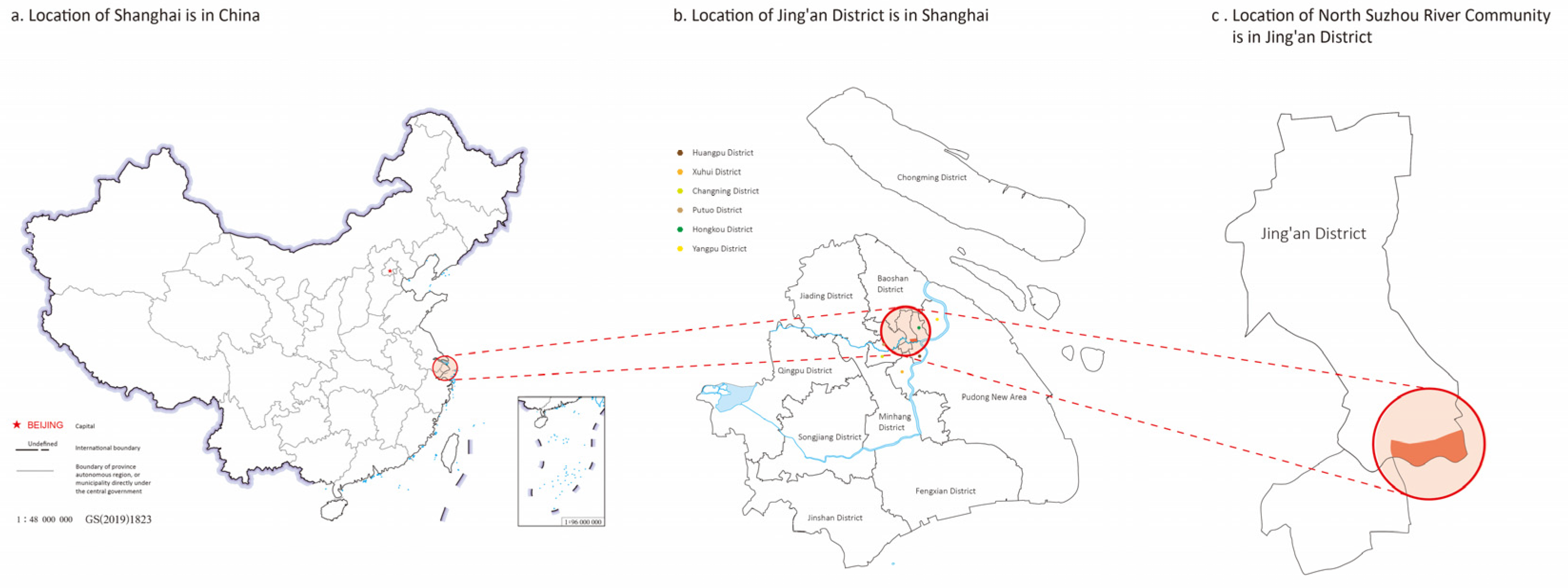
The North Suzhou River community, under the jurisdiction of the Beizhan Sub-district, is located in the southeastern part of the Jing’an District, along the northern bank of the Suzhou River (see Figure 2), adjacent to the central business district of the Bund [42]. The waterfront spans approximately 6.3 km, encompassing over 30 outstanding historically protected buildings such as the Shanghai Chamber of Commerce, the Sihang Warehouse, the Shanghai Postal Building, and the Riverside Building, making it a key route for city walking in Shanghai. According to the statistics from the sixth national population census in 2010 [43], the total population of the area is 78,000, with 32,538 permanent residents from outside the area, resulting in a 100% urbanization rate. Among the total population, the majority are of Han ethnicity, with 39,549 males (50.72%) and 38,419 females (49.28%). The age group between 15 and 64 accounts for 81.67% of the population, while those aged 65 and above comprise 11.64%. Due to its proximity to the central business district, the resident population consists mostly of employees of companies and institutions, facilitating their daily commutes. Furthermore, the Jing’an District, with the design vision of “Jing’an Suzhou Bay, the New Landmark of Shanghai,” has renovated the surrounding riverside trails, rest areas, spaces under bridges, and green landscapes. Multiple public art pieces are installed in this area to improve the quality of the space and release a more inclusive waterfront activity.
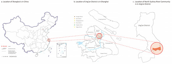
Figure 2.
The location of North Suzhou River Community. (Source: compiled by the researcher).
This is a selection of 30 public art installations in the North Suzhou River Community of Jing’an District (see Figure 3). We divided the public art into specific types and marked their locations on the map. The selected public art is mainly distributed along the north bank of Suzhou River and is located in waterfront space, historical and cultural space, green squares and commercial space. It basically includes the public art functions of environmental improvement, cultural shaping, functional services and public interaction, and is representative of both sexes.
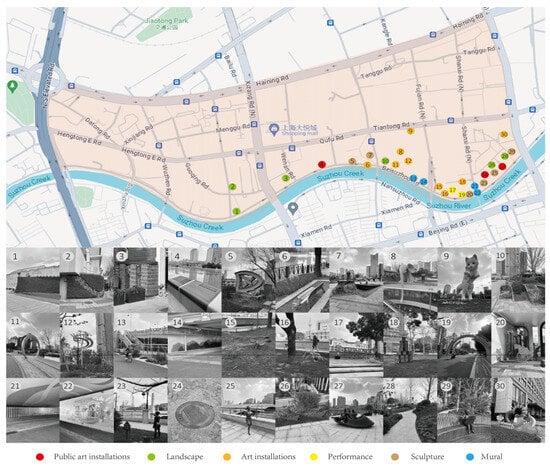
Figure 3.
The Public Art Map of North Suzhou River Community (Source: Compiled by the researcher).
4.2. Methods
Based on the literature review on the relationship between public art and pedestrian willingness, as well as field investigations, we theoretically propose that public art has a positive and significant impact on pedestrian willingness, with citizen perceived benefits serving as a mediator. The framework of this study is based on the Stimulus–Organism–Response (SOR) model, which is employed to examine how environmental stimuli generated by public art affect citizens’ perceived value, consequently influencing their urban walking choices. To validate the hypotheses, we conducted a questionnaire survey among residents of Shanghai, China, and performed a quantitative analysis based on the collected data. This study utilized CFA, a statistical analysis technique applied to social survey data [44]. Its advantage lies in allowing researchers to clearly describe the details of a theoretical model and testing whether the relationship between a factor and its corresponding measurement items conform to the theoretical relationships designed by the researchers [45]. This process is often conducted through Structural Equation Modeling (SEM). Currently, CFA is widely used in the field of sociological research.
4.3. Data Collection
As part of the empirical analysis, field research was conducted in October 2023 within the study area, specifically focusing on understanding the placement of public art and participating in public art activities within the community. The raw data used for analysis were collected through an on-site questionnaire survey conducted from 20 February to 6 March 2024. A total of 346 questionnaires were randomly distributed, out of which 315 were deemed valid. To confirm whether the respondents met the minimum sample size required for the structural equation model, the Soper [46] online free statistic calculator was utilized, based on the calculation of 29 observed variables and 10 latent variables included in the research model. The model considered an expected anticipated effect size of 0.3, a probability level of 0.05, and a desired statistical power level of 0.8. The minimum sample size for detecting effects was determined to be 190, while for the model structure it was 216, with a recommended minimum sample size of 216. Therefore, the 315 valid questionnaires exceeded the minimum sample size for respondents, meeting the requirements of the research model. One part of the questionnaire contains the basic information on the respondents, and the other part involves 10 indicators of public art, citizens’ perceived benefits, and walking intention, using a five-point Likert scale for investigation.
Based on the frequency analysis of the questionnaire data collected in Table 1, the data illustrate four distinct age groups: 15–30 years, 31–45 years, 46–60 years, and 61–75 years. Among these, the 46–60 age group constitutes the largest proportion at 36.51%, closely followed by the 31–45 age group at 31.43%. This indicates that middle-aged individuals make up the majority of the survey participants. The 15–30 and 61–75 age groups are relatively smaller, accounting for only 16.19% and 15.87%, respectively, reflecting a tendency toward middle-aged respondents. Regarding gender distribution, there is a slightly higher participation of females compared to males, but the overall difference is not significant. Analysis of occupations reveals that corporate employees constitute the largest group of survey participants, accounting for 25.08%, likely attributed to the proximity to the central business district. Regarding residency status in Shanghai, the majority of participants (77.46%) are permanent residents of Shanghai, while only 22.54% indicate non-permanent residency, mainly comprising visiting tourists. Overall, the distribution characteristics of respondents in terms of age, gender, occupation, and residency status align with the characteristics of the research area, indicating the representativeness of the sample.

Table 1.
Respondent Demographic Characteristics.
5. Empirical Results
CFA (confirmatory factor analysis) research methods and SPSS 26.0 and AMOS 24. 0 software were used for the analysis of the data from questionnaires.
5.1. Variable Descriptive Analysis
Upon analyzing the data (see Table 2), we found that the average score for the dimensions of public art was 45.181, with a median of 46, indicating a generally positive overall evaluation of public art, albeit with some variation (standard deviation of 12.961). Sub-dimensions, including environmental improvement, cultural shaping, service enhancement, and public interaction, had average scores ranging from 11.092 to 11.550, suggesting a relatively consistent perception among individuals in these aspects, leaning towards improvement. The standard deviations (ranging from 3.685 to 3.904) indicate some degree of opinion divergence, yet most individuals hold positive views regarding improvements in these areas. Regarding citizens’ perceived benefits, the average score for the functional dimension was 8.327, which is relatively high compared to the total score. The average score for willingness to walk was 11.216, with a median of 11 and a standard deviation of 3.749, indicating a preference for walking.
Table 2.
Basic indicators.
5.2. Reliability and Validity Analysis
The results of Cronbach’s reliability analysis indicate [47] that the scales of public art, citizen perceived benefits, and walking intention, along with their internal dimensions, all exhibit good to excellent internal consistency (see Table 3). The Cronbach’s α coefficients for each dimension exceed 0.8, with the scale for public art reaching over 0.9, reflecting a high level of consistency among the various indicators within the scales. This suggests that, whether assessing the impact of public art, citizen perceptions of public spaces, or measuring walking intentions, these scales demonstrate robust and reliable characteristics, providing trustworthy tools and foundations for related research endeavors.
Table 3.
Cronbach’s alpha.
The validity analysis reveals (see Table 4) that the Kaiser–Meyer–Olkin (KMO) values for the scales of public art, citizen perceived benefits, and walking intention are 0.913, 0.875, and 0.775, respectively, indicating that these data are highly suitable for factor analysis. The high KMO values imply strong correlations among the variables within these scales, facilitating the exploration of underlying factors through factor analysis [48]. Particularly noteworthy are the high KMO values for the scales of public art and citizen-perceived benefits, underscoring their suitability for probing the latent factor structure. Although the suitability of the walking intention scale is slightly lower, it still possesses a high KMO value, enabling factor analysis to delve into its underlying factors. These findings provide robust data foundations for further research endeavors.
Table 4.
Validity analysis.
5.3. Confirmatory Factor Analysis
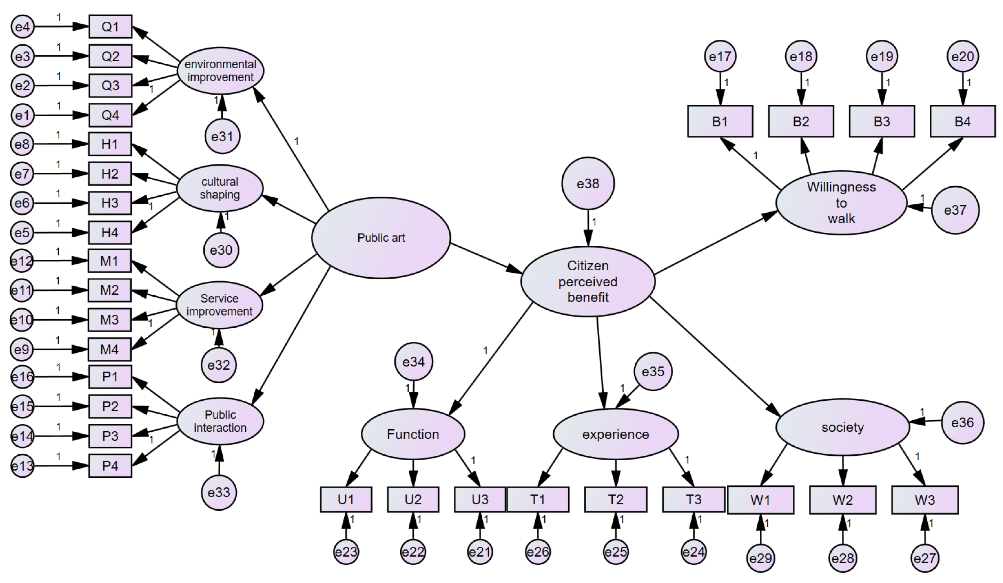
The data presented herein indicate a CFA (see Figure 4) aimed at assessing the relationships among multiple constructs (such as public art, citizen perceived benefits, and walking intention) and their respective observed variables (such as environmental improvement, cultural shaping, service enhancement and public interaction). CFA is a key component of SEM, used to verify whether the preconceived theoretical structure holds true in the observed data.
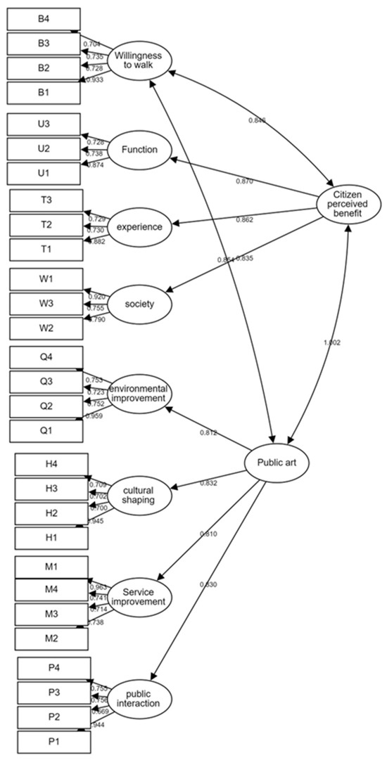
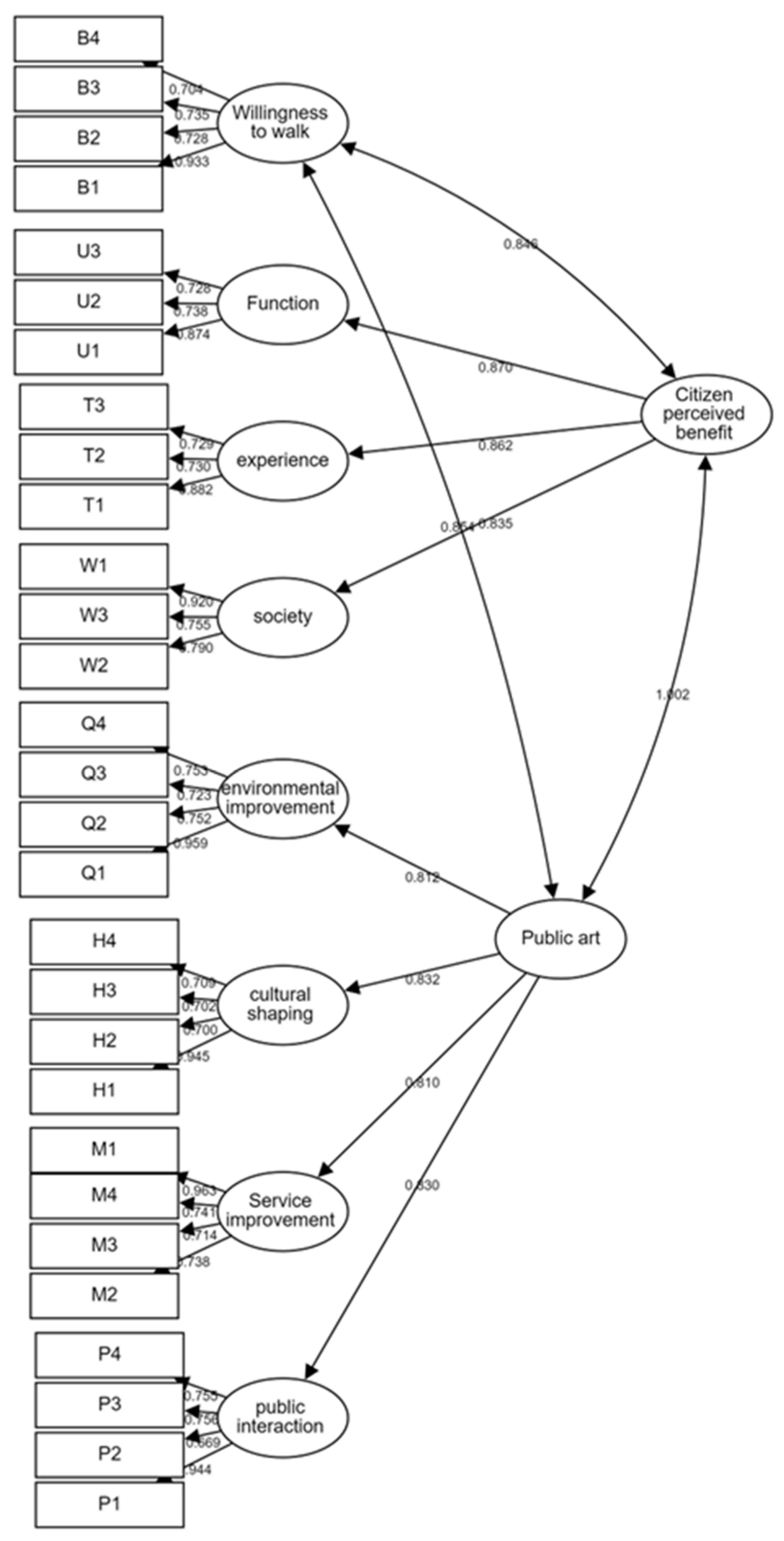
Figure 4.
Unstandardized estimate of the SEM model. (The arrows denote the direction of influence or causality, indicating the association between latent variables and observed variables. The numbers represent the standardized regression coefficients).
The construct of public art exhibits strong influences on its downstream variables (environmental improvement, cultural shaping, service enhancement, public interaction), with standardized regression coefficients (β) ranging from 0.81 to 0.832 (see Table 5). The overall average variance extracted (AVE) value is 0.674, and the composite reliability (CR) value is 0.892, indicating good convergent validity and reliability. Similarly, the construct of citizen-perceived benefits demonstrates significant impacts on the functional, experiential, and social dimensions (standardized regression coefficients ranging from 0.835 to 0.87), with an AVE value of 0.732 and a CR value of 0.891, also indicating good convergent validity and internal consistency.
Table 5.
Confirmatory Factor Analysis.
Regarding the downstream variables, each dimension shows strong explanatory power for its observed variables. Particularly noteworthy are the high standardized regression coefficients (β) for environmental improvement in Q1, cultural shaping in H1, and service enhancement in M1, all approaching or exceeding 0.9, indicating strong associations with their corresponding constructs.
Overall, most constructs exhibit AVE values exceeding the threshold of 0.5, and CR values surpassing the acceptable standard of 0.7, indicating good convergent validity and internal consistency of the data, thereby validating the adaptability of the theoretical model to the data. The results of this CFA support the hypothesized relationships between the predefined constructs and their corresponding observed variables in the research model, demonstrating a solid theoretical foundation and empirical support for the model.
The table presents correlation coefficients among a series of variables (see Table 6), along with the square root of the Average Variance Extracted (AVE) for each variable, commonly used in SEM to assess the discriminant validity of constructs. Discriminant validity refers to the distinction between different constructs and whether each construct captures information distinct from other constructs. A commonly used criterion is that the square root of the AVE for each construct should be greater than the correlations of that construct with other constructs in the model in order to demonstrate good discriminant validity [49].
Table 6.
Discriminant validity: Pearson correlation and AVE square root value.
The values on the diagonal represent the square root of the AVE for each construct. This value should be greater than the correlation of that construct with any other construct in order to demonstrate discriminant validity [50]. Correlation coefficients between constructs, denoted by asterisks (**), indicate statistically significant correlations. It can be observed from the table that the square roots of the AVE for the constructs of public art, citizen-perceived benefits, and walking intention are 0.821, 0.787, and 0.780, respectively. Moreover, all correlations associated with these constructs are lower than the square roots of the corresponding AVEs, meeting the requirements for discriminant validity. These constructs are effectively differentiated, each capturing unique information, aiding in a clear interpretation of different factors in the research model. Such clarity in differentiation is crucial for understanding the relationships between different variables and how they influence research outcomes.
The comprehensive analysis reveals that the model fits well and is applicable (see Table 7). The model’s χ2 value is 485.307 with 366 degrees of freedom, resulting in a chi-square to degrees of freedom ratio of 1.326. The ratio of χ2/df, being below three, indicates a good fit of the model. Although the p-value of the χ2 test is significant, in the case of large samples, this value may be overly sensitive to minor deviations. The Goodness-of-Fit Index (GFI) exceeds 0.9, the Root Mean Square Error of Approximation (RMSEA) is well below 0.10, and the Root Mean Square Residual (RMR) is close to the threshold for a good fit, indicating a good fit of the model to the data. The Comparative Fit Index (CFI), Normed Fit Index (NFI), Non-Normed Fit Index (NNFI), Tucker–Lewis Index (TLI), and Incremental Fit Index (IFI) all exceed the standard of 0.9 for good model fit, while the Adjusted Goodness-of-Fit Index (AGFI) is slightly lower but still close to the good fit criterion. The Parsimonious Goodness-of-Fit Index (PGFI), Parsimonious Normed Fit Index (PNFI), and Parsimonious Comparative Fit Index (PCFI) all exceed the standard of 0.5, indicating good parsimony of the model. The Standardized Root Mean Square Residual (SRMR) is below 0.1, and the 90% confidence interval for RMSEA further confirms the stability and excellence of the results. In summary, the model is deemed appropriate for practical application.
Table 7.
Model fit indices.
5.4. Correlation Analysis
The table (see Table 8) presents correlation coefficients among different variables, with values of 1 along the diagonal, indicating perfect correlation of each variable with itself. The asterisks (**), appearing in the table, denote statistically significant correlations, suggesting meaningful relationships between these variables. Analyzing these correlations allows for a deeper understanding of the relationships among variables.
Table 8.
Correlation analysis.
Public art exhibits generally high correlations with other dimensions, particularly with EI (0.854) and CPB (0.855), indicating a close association between public art and these domains. This suggests that the development of public art significantly influences environmental enhancement and the social benefits perceived by citizens. EI shows correlations with CS, SI, and PI (around 0.632), all of which are statistically significant, indicating a certain degree of connection between environmental improvement and cultural, service, and public interaction aspects. Citizen-perceived benefits exhibit correlations with functionality and experience, indicating that citizens’ perception of social benefits depends on improved functionality and positive experiences. The correlation coefficients between WTW and other dimensions are relatively consistent, ranging from 0.631 to 0.742. This reflects a certain association between WTW and aspects such as PA, EI, and CS.
5.5. Path Analysis
χ2/df: The value of 1.317, significantly below the standard threshold of three, indicates a good model fit. This is an important indicator for evaluating the overall goodness of fit of the model, with values below three typically indicating a good fit between the model and the data (see Figure 5).
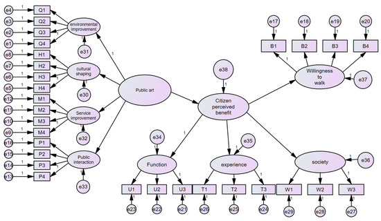
Figure 5.
Path analysis diagram. (The arrows represent the direction of influence or causality between variables).
GFI: With a value of 0.909, meeting the criterion of >0.9 for good fit, indicates a well-fitted model with the observed data.
RMSEA: At 0.032, well below the threshold of 0.10, suggests a small model error and excellent fit.
RMR: With a value of 0.050, close to the ideal threshold of <0.05, indicates small residuals and a high degree of fit between the model and the data.
CFI, NFI, NNFI: These indices all exceed the threshold of 0.9 for good fit, with values of 0.980, 0.922, and 0.978, respectively, indicating very good relative fit of the model.
TLI and IFI: Similar to NNFI, TLI has a value of 0.978, and IFI has a value of 0.980, both surpassing the good fit threshold of 0.9, further confirming the excellent fit of the model.
AGFI: Slightly increased to 0.893, and slightly below the ideal value of 0.9 but close to it, this indicates a good fit between the model and the data even after considering model complexity.
PGFI, PNFI, and PCFI: These indices consider the parsimony of the model, with values of 0.769, 0.836, and 0.888, respectively, all exceeding the threshold of 0.5, indicating good fit of the model while maintaining reasonable complexity.
SRMR: With a value of 0.041, below the threshold of 0.1, this indicates small residuals and good fit.
RMSEA 90% CI (RMSEA 90% Confidence Interval): Ranging from 0.023 to 0.039, this narrow confidence interval further confirms the stability and excellence of the RMSEA results.
Based on these fit indices (see Table 9), it can be concluded that the model has an excellent fit. Almost all indices meet or exceed their respective criteria for good fit, indicating that the model adequately reflects the structural relationships in the data. Although the p-value from the χ2 test indicates a statistically significant difference between the model and perfect fit, this is common in large-sample studies [51]. Considering that other fit indices all demonstrate good model fit, it can be deemed that this model is appropriate for practical application.
Table 9.
Model fit index.
The summary table of regression coefficients (Table 10) provides a detailed overview of the relationships between variables, including Standard Error (SE), CR, p-values, and standardized regression coefficients. Analyzing these data allows us to understand how variables interact within the model, as well as the statistical significance and strength of these interactions [52].
Table 10.
Model regression coefficient summary table.
Standardized regression coefficients indicate the change in the standard deviation of the dependent variable Y when the independent variable X changes by one standard deviation [53]. Higher values suggest a stronger impact. Standard Error (SE) reflects the precision of the estimates, while CR is used to test hypotheses, with higher z-values indicating statistically significant regression coefficients [54]. The p-value is used to assess the significance of the regression coefficients, typically with p < 0.05 indicating statistical significance [55].
The impact of public art on citizens perceived benefits is manifested by a standardized regression coefficient of 1, indicating a very strong positive effect, and it is highly significant statistically (p = 0). The effect of citizen perceived benefits on walking intention is represented by a standardized regression coefficient of 0.84, indicating a strong positive effect, and similarly it is highly significant statistically (p = 0).
In other aspects, the influence of public art on environmental improvement, cultural shaping, service enhancement, and public interaction is highly significant, with standardized regression coefficients of 0.802, 0.829, 0.807, and 0.826, respectively. Similarly, the impact of citizens’ perceived benefits on functionality, experience, and social aspects is also highly significant, with standardized regression coefficients of 0.86, 0.857, and 0.83, respectively.
6. Discussion
The empirical findings indicate that these data reveal significant and intricate associations among various social and environmental dimensions, such as public art, environmental improvement, and citizen-perceived benefits. Particularly, the high correlation between public art and environmental improvement, as well as citizen-perceived benefits, underscores the crucial role of art in urban development and resident well-being. Additionally, the association between citizens’ perceived benefits and functionality and experience highlights the importance of these factors in enhancing the quality of urban life. Life circle planning with a 15-min radius emphasizes the connection between production, living space and behavior habits, effectively allocates public resources, improves service efficiency, inspires a new low-carbon lifestyle in the post-epidemic era, and enhances the climate adaptability of urban development and public life [56]. So far, the practice of the “15-min” CLC in Shanghai has made good progress. However, in terms of building a sustainable urban system in the future, the current practice in Shanghai is still in the early stages. Building upon this foundation, to encourage individuals to actively choose urban walking as a response to energy and emissions challenges and to achieve sustainable urban development, this study offers important practical insights. Firstly, in the realm of public art, attention should be directed towards enhancing perceived functionality to elevate overall citizen satisfaction. Secondly, considering the proximity of scores between pedestrian willingness and public interaction, this may imply that public space design and activities have a positive impact on community walking and interaction. Further exploration of the correlation between these and the enhancement of pedestrian willingness through improved public space design and services are warranted. Lastly, enhancing the score of the cultural shaping dimension through measures such as boosting art exhibitions and cultural activities, or increasing convenience facilities and services to elevate satisfaction in the functionality dimension, should be considered.
Public art and citizen-perceived benefits play central roles in the model, exhibiting significant positive effects on other variables and being closely associated with citizen-urban empowerment and community engagement. The findings from our study underscore the critical importance of integrating public art into urban environments to foster healthy lifestyle choices, particularly in promoting activities like walking. Encouraging walking frequency through the incorporation of public art not only contributes to individual well-being but also holds broader implications for urban sustainability efforts. By reducing reliance on cars, walking promotes a greener and healthier urban lifestyle, aligning with objectives aimed at mitigating carbon emissions and enhancing environmental sustainability. Furthermore, the integration of public art into urban spaces provides valuable insights for urban planners and policymakers in designing effective intervention measures. By strategically placing art installations in pedestrian-friendly areas, cities can not only enhance the aesthetic appeal of public spaces but also encourage active modes of transportation, thereby contributing to the promotion of green and healthy lifestyles. These findings offer valuable perspectives on urban sustainable planning, emphasizing the importance of incorporating artistic elements into urban design strategies. By leveraging public art as a tool for community engagement and empowerment, cities can create more vibrant and livable environments while simultaneously advancing efforts to reduce carbon emissions and promote sustainable urban development.
In this study, we employed the SOR model to construct and validate a conceptual framework for the influence of public art on urban walking choices, providing a novel perspective on the study of pedestrian willingness. Using the CFA analysis method, we empirically tested the impact of the dimensions of public art and citizen perception on pedestrian willingness, thereby expanding the scope of research on public art. However, regarding the future establishment of sustainable urban transportation networks and 15-min CLCs, the current practice in Shanghai is still in its infancy. There are several issues concerning the installation of public art, such as the lack of systematic management procedures, uneven distribution across regions, low citizen awareness, and weak participation. Therefore, there is a need for strengthened policy incentives to systematically support diverse development of public art, encouraging community residents to participate in the selection, planning, and management processes of public art, thereby enhancing residents’ perception of the benefits of public art and increasing its attractiveness. This will help further highlight the locality, public nature, and participatory characteristics of public art, promoting urban sustainable development and the creation of more livable urban environments.
7. Conclusions
This study investigates the influence of public art on urban walking choices through a case analysis of the North Suzhou River Community Living Circle in Jing’an District, Shanghai. A conceptual framework based on the SOR theory is constructed. Empirical results demonstrate that, in the construction of the 15-min CLC, the installation of public art positively influences people’s walking choices, with citizen perception acting as a crucial mediator. Thus, enhancing urban residents’ experiences, functional satisfaction, and perception of social value in the urban environment will promote the likelihood of people choosing walking as a mode of transportation. This, in turn, will facilitate the bottom-up formation of dense green transportation networks to address climate challenges and promote urban sustainable development.
Future research will delve deeper into the relationship between public art and urban walking choices, exploring various aspects. Firstly, the research will investigate the mechanism through which public art influences urban walking choices, including factors such as the design features of public art, its placement, artistic forms, and how these factors affect urban residents’ willingness and behavior to walk. Secondly, attention will be given to understanding the differential impact of public art on walking choices in different community environments, considering factors such as geographical conditions, population structure, and cultural atmosphere to provide a basis for tailored strategies for public art installation. Lastly, interdisciplinary collaboration will be emphasized to integrate expertise from fields such as art, urban planning, sociology, etc., to advance the deep integration of public art and urban sustainable development, contributing to the creation of green, healthy, and livable urban environments. These research directions will provide theoretical guidance and practical support for achieving sustainable urban development and constructing more livable urban environments.
Author Contributions
Conceptualization, R.T.; materials and methods, R.T. and Y.W.; formal analysis, R.T. and Y.W.; writing—original draft preparation, R.T.; writing—review and editing, R.T., Y.W. and S.Z.; supervision, S.Z.; funding acquisition, S.Z. All authors have read and agreed to the published version of the manuscript.
Funding
This research has received funding from Art Project of the National Social Science Foundation [No.18BG116].
Institutional Review Board Statement
Not applicable.
Informed Consent Statement
Informed consent was obtained from all subjects involved in the study.
Data Availability Statement
The data presented in this study are available on request from the corresponding author. Data are not publicly available due to the privacy terms signed by the respondents in the informed consent.
Conflicts of Interest
The authors declare no conflicts of interest.
References
- United Nations. World Urbanization Prospects: The 2007 Revision Population Database; United Nations: New York, NY, USA, 2008. [Google Scholar]
- Moreno, C.; Allam, Z.; Chabaud, D.; Gall, C.; Pratlong, F. Introducing the “15-Minute City”: Sustainability, Resilience and Place Identity in Future Post-Pandemic Cities. Smart Cities 2021, 4, 93–111. [Google Scholar] [CrossRef]
- Shanghai Municipal People’s Government. Shanghai Master Plan (2017–2035); Shanghai Municipal People’s Government: Shanghai, China, 2018.
- Shanghai Urban Planning and Land Resources Administration Bureau. Shanghai Planning Guidance of 15-Minute Community-Life Circle; Shanghai Urban Planning and Land Resources Administration Bureau: Shanghai, China, 2016. [Google Scholar]
- Cartiere, C.; Willis, S. The Practice of Public Art; Taylor Francis: Oxfordshire, UK, 2008; Available online: https://books.google.com.au/books?id=f6mTAgAAQBAJ (accessed on 10 July 2023).
- Southworth, M. Designing the Walkable City. J. Urban Plan. Dev. 2005, 131, 246–257. [Google Scholar] [CrossRef]
- Páez, A.; Whalen, K. Enjoyment of commute: A comparison of different transportation modes. Transp. Res. Part A Policy Pract. 2010, 44, 537–549. [Google Scholar] [CrossRef]
- Giles-Corti, B.; Broomhall, M.H.; Knuiman, M.; Collins, C.; Douglas, K.; Ng, K.; Lange, A.; Donovan, R.J. Increasing walking: How important is distance to, attractiveness, and size of public open space? Am. J. Prev. Med. 2005, 28 (Suppl. S2), 169–176. [Google Scholar] [CrossRef]
- Owen, N.; Humpel, N.; Leslie, E.; Bauman, A.; Sallis, J.F. Understanding environmental influences on walking: Review and research agenda. Am. J. Prev. Med. 2004, 27, 67–76. [Google Scholar] [CrossRef] [PubMed]
- Jabareen, Y. Planning the resilient city: Concepts and strategies for coping with climate change and environmental risk. Cities 2013, 31, 220–229. [Google Scholar] [CrossRef]
- Xiao, Z.; Chai, W.; Yan, Z. Overseas Life Circle Planning And Practice. Planners 2014, 30, 89–95. [Google Scholar]
- Al-Hindi, K.F.; Till, K.E. (RE)Placing the New Urbanism Debates: Toward an Interdisciplinary Research Agenda. Urban Geogr. 2001, 22, 189–201. [Google Scholar] [CrossRef]
- Mulíček, O.; Osman, R.; Seidenglanz, D. Urban rhythms: A chronotopic approach to urban timespace. Time Soc. 2014, 24, 304–325. [Google Scholar] [CrossRef]
- Moreno, C. La ville du Quart D’heure: Pour un Nouveau Chrono-Urbanisme! 2016. Available online: https://www.latribune.fr/regions/smart-cities/la-tribune-de-carlos-moreno/la-ville-du-quart-d-heure-pour-un-nouveau-chrono-urbanisme-604358.html (accessed on 5 February 2022).
- Kecheng, Z.; Hussain, M. The Historical Origin and Public Manifestation of Public Art. Pak. Soc. Sci. Rev. 2023, 7, 61–71. [Google Scholar] [CrossRef]
- Becker, J. Public Art: An Essential Component of Creating Communities; Americans for the Arts: Washington, DC, USA, 2004. [Google Scholar]
- Cervero, R.; Transit Cooperative Research Program. Transit-Oriented Development in the United States: Experiences, Challenges, and Prospects; Transportation Research Board: Washington, DC, USA, 2004; Available online: https://books.google.com.au/books?id=a6__pNpM44MC (accessed on 15 October 2023).
- Knight, C.K. Public Art: Theory, Practice and Populism; Wiley: Hoboken, NJ, USA, 2011; Available online: https://books.google.com.au/books?id=qkxClDeTCbQC (accessed on 20 July 2023).
- Finkelpearl, T.; Acconci, V. Dialogues in Public Art; MIT Press: Cambridge, MA, USA, 2000; Available online: https://books.google.com.au/books?id=T51F3wYglToC (accessed on 20 July 2023).
- Communications, D.O.; Arts, T. Creative Nation: Commonwealth Cultural Policy, October 1994. 2003. Available online: https://webarchive.nla.gov.au/awa/20031203235148/http://www.nla.gov.au/creative.nation/contents.html (accessed on 20 May 2022).
- Stevenson, D.; Magee, L. Art and space: Creative infrastructure and cultural capital in Sydney, Australia. J. Sociol. 2017, 53, 839–861. [Google Scholar] [CrossRef]
- Talen, E. Sense of Community and Neighbourhood Form: An Assessment of the Social Doctrine of New Urbanism. Urban Stud. 1999, 36, 1361–1379. [Google Scholar] [CrossRef]
- Kellerman, A. Personal Mobilities; Taylor Francis: Oxfordshire, UK, 2006; Available online: https://books.google.com.au/books?id=ta1-AgAAQBAJ (accessed on 20 July 2023).
- Howard, E. Garden Cities of To-Morrow, 1st ed.; Osborn, F.J., Ed.; Routledge: London, UK, 2016. [Google Scholar] [CrossRef]
- Corbusier, L. The City of To-Morrow and Its Planning; Dover: Grove, IL, USA, 1987; Available online: https://books.google.com.au/books?id=FknLsAm7R_YC (accessed on 15 October 2023).
- Dempsey, N.; Brown, C.; Bramley, G. The key to sustainable urban development in UK cities? The influence of density on social sustainability. Prog. Plan. 2012, 77, 89–141. [Google Scholar] [CrossRef]
- Guan, C.; Keith, M.; Hong, A. Designing walkable cities and neighborhoods in the era of urban big data. Urban Plan. Int. 2020, 34. [Google Scholar] [CrossRef]
- Kopec, D. Environmental Psychology for Design: With STUDIO; Bloomsbury Publishing: London, UK, 2018; Available online: https://books.google.com.au/books?id=YdHWEAAAQBAJ (accessed on 3 June 2023).
- Gehl, J.; He, R. Life between Buildings; China Architecture Building Press: Beijing, China, 1992. [Google Scholar]
- Mehrabian, A.; Russell, J.A. A verbal measure of information rate for studies in environmental psychology. Environ. Behav. 1974, 6, 233. [Google Scholar]
- Foa, E.B.; Steketee, G.; Rothbaum, B.O. Behavioral/cognitive conceptualizations of post-traumatic stress disorder. Behav. Ther. 1989, 20, 155–176. [Google Scholar] [CrossRef]
- Koppes, L.L. Historical Perspectives in Industrial and Organizational Psychology; Taylor Francis: Oxfordshire, UK, 2014; Available online: https://books.google.com.au/books?id=vJ3KAgAAQBAJ (accessed on 20 July 2023).
- Panksepp, J. Affective consciousness: Core emotional feelings in animals and humans. Conscious. Cogn. 2005, 14, 30–80. [Google Scholar] [CrossRef]
- Ledoux, J.E. Cognitive-Emotional Interactions in the Brain. Cogn. Emot. 1989, 3, 267–289. [Google Scholar] [CrossRef]
- Sharp, J.; Pollock, V.; Paddison, R. Just art for a just city: Public art and social inclusion in urban regeneration. In Culture-Led Urban Regeneration; Routledge: London, UK, 2020; pp. 156–178. [Google Scholar]
- Nguyen, M.H.; Khoa, B.T. Perceived Mental Benefit in Electronic Commerce: Development and Validation. Sustainability 2019, 11, 6587. [Google Scholar] [CrossRef]
- Chiesura, A. The role of urban parks for the sustainable city. Landsc. Urban Plan. 2004, 68, 129–138. [Google Scholar] [CrossRef]
- Larranaga, A.M.; Arellana, J.; Rizzi, L.I.; Strambi, O.; Cybis, H.B.B. Using best–worst scaling to identify barriers to walkability: A study of Porto Alegre, Brazil. Transportation 2019, 46, 2347–2379. [Google Scholar] [CrossRef]
- Miles, M. Art, Space and the City; Routledge: London, UK, 2005. [Google Scholar]
- McCarthy, J. Regeneration of Cultural Quarters: Public Art for Place Image or Place Identity? J. Urban Des. 2006, 11, 243–262. [Google Scholar] [CrossRef]
- Deutsche, R. Art and Public Space: Questions of Democracy. Soc. Text 1992, 33, 34–53. [Google Scholar] [CrossRef]
- Jing’an District People’s Government, Shanghai Municipality. Profile of Jing’an; Jing’an District People’s Government, Shanghai Municipality: Shanghai, China, 2023. Available online: https://english.jingan.gov.cn/qq/004001/foreign-singledetail.html (accessed on 15 June 2023).
- National Bureau of Statistics of China. Regional Division of Beizhan Street in 2021; National Bureau of Statistics of China: Beijing, China, 2021. Available online: https://www.stats.gov.cn/tjsj/tjbz/tjyqhdmhcxhfdm/2021/31/01/06/310106016.html (accessed on 5 May 2022).
- Brown, T.A. Confirmatory Factor Analysis for Applied Research, 2nd ed.; Guilford Publications: New York, NY, USA, 2015. [Google Scholar]
- Hurley, A.E.; Scandura, T.A.; Schriesheim, C.A.; Brannick, M.T.; Seers, A.; Vandenberg, R.J.; Williams, L.J. Exploratory and Confirmatory Factor Analysis: Guidelines, Issues, and Alternatives. J. Organ. Behav. 1997, 18, 667–683. [Google Scholar] [CrossRef]
- Soper, D.S. A-Priori Sample Size Calculator for Structural Equation Models [Software]. 2024. Available online: https://www.danielsoper.com/statcalc (accessed on 15 October 2023).
- Peterson, R.A. A Meta-analysis of Cronbach’s Coefficient Alpha. J. Consum. Res. 1994, 21, 381–391. [Google Scholar] [CrossRef]
- Watkins, M.W. Exploratory Factor Analysis: A Guide to Best Practice. J. Black Psychol. 2018, 44, 219–246. [Google Scholar] [CrossRef]
- Henseler, J.; Ringle, C.M.; Sarstedt, M. A new criterion for assessing discriminant validity in variance-based structural equation modeling. J. Acad. Mark. Sci. 2015, 43, 115–135. [Google Scholar] [CrossRef]
- Ab Hamid, M.R.; Sami, W.; Mohmad Sidek, M.H. Discriminant Validity Assessment: Use of Fornell & Larcker criterion versus HTMT Criterion. J. Phys. Conf. Ser. 2017, 890, 012163. [Google Scholar] [CrossRef]
- Schermelleh-Engel, K.; Moosbrugger, H.; Müller, H. Evaluating the fit of structural equation models: Tests of significance and descriptive goodness-of-fit measures. Methods Psychol. Res. Online 2003, 8, 23–74. [Google Scholar]
- Menard, S. Applied Logistic Regression Analysis; SAGE Publications: Washington, DC, USA, 2002; Available online: https://books.google.com.au/books?id=EAI1QmUUsbUC (accessed on 30 July 2023).
- Clogg, C.C.; Petkova, E.; Haritou, A. Statistical Methods for Comparing Regression Coefficients Between Models. Am. J. Sociol. 1995, 100, 1261–1293. [Google Scholar] [CrossRef]
- Franzese, R.; Kam, C. Modeling and Interpreting Interactive Hypotheses in Regression Analysis; University of Michigan Press: Ann Arbor, MI, USA, 2009; Available online: https://books.google.com.au/books?id=1RTNDZcreVkC (accessed on 30 July 2023).
- Greenland, S.; Senn, S.J.; Rothman, K.J.; Carlin, J.B.; Poole, C.; Goodman, S.N.; Altman, D.G. Statistical tests, P values, confidence intervals, and power: A guide to misinterpretations. Eur. J. Epidemiol. 2016, 31, 337–350. [Google Scholar] [CrossRef] [PubMed]
- Pozoukidou, G.; Chatziyiannaki, Z. 15-Minute City: Decomposing the New Urban Planning Eutopia. Sustainability 2021, 13, 928. [Google Scholar] [CrossRef]

Disclaimer/Publisher’s Note: The statements, opinions and data contained in all publications are solely those of the individual author(s) and contributor(s) and not of MDPI and/or the editor(s). MDPI and/or the editor(s) disclaim responsibility for any injury to people or property resulting from any ideas, methods, instructions or products referred to in the content. |
© 2024 by the authors. Licensee MDPI, Basel, Switzerland. This article is an open access article distributed under the terms and conditions of the Creative Commons Attribution (CC BY) license (https://creativecommons.org/licenses/by/4.0/).