Measuring Labor Market Status Using Remote Sensing Data

Abstract

In this study, we utilize remote sensing data to estimate employment in Bangladesh. Since labor force surveys are only conducted occasionally in Bangladesh, total employment is measured statistically based on scarce survey data. To exploit the real-time availability and regionally subdivided characteristic of remote sensing data, we estimated annual employment in terms of job quality in 64 districts using interpolation. Using the employment data interpolated by job quality, which show how many people have good-quality employment, such as a good employer or regular-paid job, we constructed a forecasting model for annual employment data with mixed frequency control variables in quarterly frequency, as well as remote sensing data. Then, we extended the model for estimating quarterly employment status using a monthly series, which included remote sensing data such as nighttime light and enhanced vegetation index. Since there was no true observation in our target variable, there was no way to verify the accuracy of the forecasting model. Instead, we extended our approach to perform an out-of-sample forecast, since we had real-time data up to the first half of 2022. As a result, the remote sensing data may not have captured the overall trend of employment due to the domination of control variables such as industrial production. However, the remote sensing data showed idiosyncratic movement by districts. Therefore, our result is helpful for policymakers in implementing labor policies for specific districts because it allows for observing remote sensing data trends in real time.

1. Introduction

Ensuring decent work and economic growth, as emphasized by United Nations Sustainable Development Goal (SDG) 8, is a crucial aspect of sustainable development. However, in many low- and middle-income countries, labor market indicators are published with considerable time lags or are based on infrequent, small-scale surveys. Bangladesh, in particular, faces significant challenges in obtaining timely labor market statistics due to relatively weak statistical infrastructure and limited resources for frequent nationwide surveys. Consequently, policymakers often lack near-real-time data to detect shifts in employment status or job quality—a limitation that can hinder timely interventions for equitable development.

In response to these data challenges, remote sensing techniques have emerged as a promising alternative or complement to traditional statistical sources. Satellite-derived measures including nighttime light (NTL) and the enhanced vegetation index (EVI) offer granular, regularly updated information on economic and environmental changes, which can be mapped at local levels and aggregated as needed. These remote sensing proxies have demonstrated potential in various domains, including monitoring deforestation [1], estimating regional production [2], and gauging economic activity where official data are sparse [3]. Recent studies in Bangladesh also suggest the feasibility of correlating remotely sensed indicators with labor or population trends [4,5].

Building on these insights, this study leverages remote sensing data and established macroeconomic indicators to measure and forecast the labor market conditions in Bangladesh. Specifically, we focus on three main objectives:

• Interpolation of Sparse Survey Data. As Bangladesh’s Labor Force Survey (LFS) has only been conducted intermittently (e.g., 2005–2006, 2013, and 2015–2016) [6,7,8] we employ interpolation strategies [9] to generate more continuous annual and quarterly proxies for labor market outcomes, allowing us to fill data gaps and gain insights into trends that are potentially overlooked by traditional methods.
• Integration of High-Frequency Remote Sensing Data. To capitalize on the real-time capabilities of remote sensing, we incorporate monthly observations of NTL and EVI into our forecasting framework. While macroeconomic series like industrial production indices are updated quarterly or annually, satellite imagery is often available at much higher frequencies, enabling us to detect sudden shifts in local economic conditions.
• Mixed-Frequency Forecasting (MIDAS) and Comparison with Traditional Models. We adopt a MIDAS approach [10], which integrates various data frequencies into a single model, enabling higher-resolution tracking of employment trends. Additionally, we compare our forecasts to a traditional ARIMA baseline, emphasizing how remote sensing variables can reveal district-level idiosyncrasies often overlooked by aggregate-only models.

1.1. Research Purpose and Motivation

This study addresses the policy need for timelier and spatially disaggregated labor market statistics. Policymakers in Bangladesh frequently require up-to-date metrics of employment trends to shape public initiatives, especially in regions where structural transformations—from agriculture to manufacturing or services—are accelerating. Relying solely on sporadic national surveys risks underestimating rapid local changes or missing critical early signals of evolving employment quality.

Furthermore, addressing labor market data gaps through remote sensing aligns with broader sustainability objectives. If local authorities can monitor which districts experience sudden declines in formal employment (e.g., due to climate disruptions or policy changes), they can allocate resources, more effectively foster the creation of decent work opportunities, and reduce economic vulnerabilities, thereby supporting SDG 8. In this context, real-time satellite observations complement official data and strengthen the foundation for sustainable labor policies at both the national and subnational levels.

1.2. Organization of This Paper

Following the Introduction, Section 2 details the data sources, including survey-based labor market variables, satellite-derived indicators, and macroeconomic controls. Section 3 outlines the methodological framework, discussing the interpolation of limited LFS data, the MIDAS setup, the rationale for incorporating remote sensing and standard macroeconomic variables. Section 4 presents the empirical results, including in-sample estimates, out-of-sample forecasts extending to 2022, and a comparative discussion contrasting the mixed-frequency approach with a simpler ARIMA model. Section 5 concludes by summarizing the key findings, reflecting on the limitations of out-of-sample predictions in data-scarce settings and proposing avenues for future research, such as integrating climate or thermal remote sensing indices to analyze informal and agricultural employment.

This study integrates high-frequency satellite imagery, macroeconomic indicators, and LFS data to reveal how real-time spatial data can enhance policy responsiveness in labor markets that are otherwise handicapped by reporting delays and incomplete statistics. The following section presents the datasets and explains their assembly for the subsequent mixed-frequency analysis.

2. Data

To forecast the labor market status in Bangladesh, we assemble multiple survey-based and remotely sensed data sources. Our overarching goal is to construct a time series of employment indicators that captures the country’s intrayear dynamics while also supporting sustainable development strategies under SDG 8. This section describes how we address the limitations inherent in sporadic data availability by combining (i) LFS data and other socioeconomic statistics, (ii) satellite-based indicators, and (iii) macroeconomic controls to address the limitations inherent in sporadic data availability.

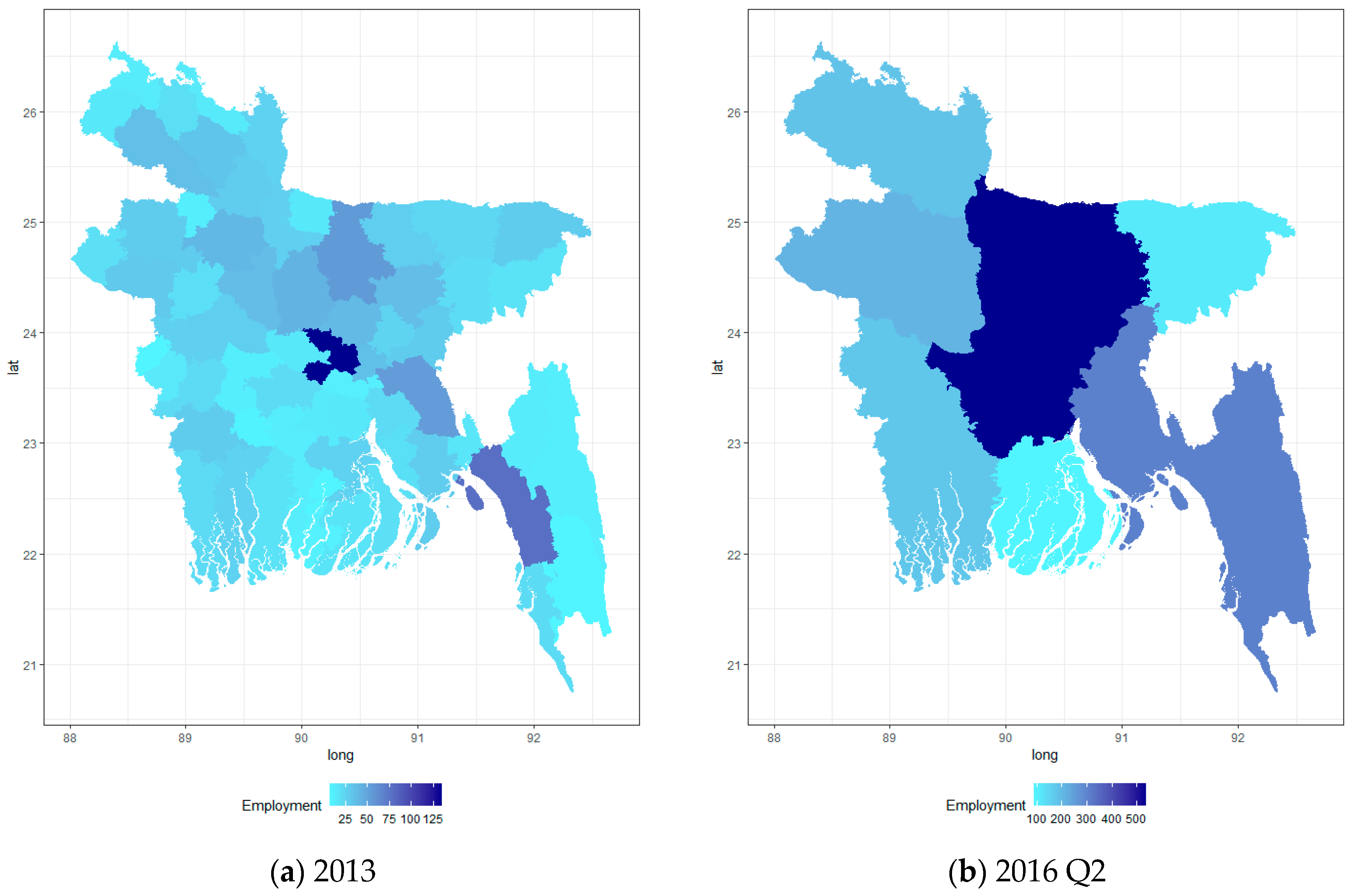
2.1. Survey-Based Employment Measures

Our target variable is employment obtained from the LFS conducted by the Bangladesh Bureau of Statistics (BBS) in three periods, 2005–2006, 2013, and 2015–2016, for 64 districts (zila). Additionally, we identified more socioeconomic variables, such as per capita income, per capita expenditure, and housing type by territory, from the Income and Expenditure Survey (HIES). Figure 1 illustrates total employment by division based on the LFS in 2013 and the second quarter of 2016 (note that there are no district-level data and the province “Mymensingh” is missing in the survey of 2016). Employment levels are highest in Dhaka because Dhaka is the most densely populated district. Chittagong, the second-most-populated district of Bangladesh, also has a high employment level. In the more populated areas, we anticipate better employment opportunities, defined as a regularly paid job, self-employment opportunities (not in agriculture) or employers (not in agriculture); thus, we also expect those areas to reflect more NTLs.

Figure 2 illustrates the Bangladesh population in the 2011 census and the expected population for 2021. It is confirmed that Figure 1 and Figure 2 show almost similar shapes, when compared with the 2013 LFS.

2.2. Satellite-Derived Indicators

To capture real-time or near-real-time changes in local economic activity, we incorporate the following remote sensing data:

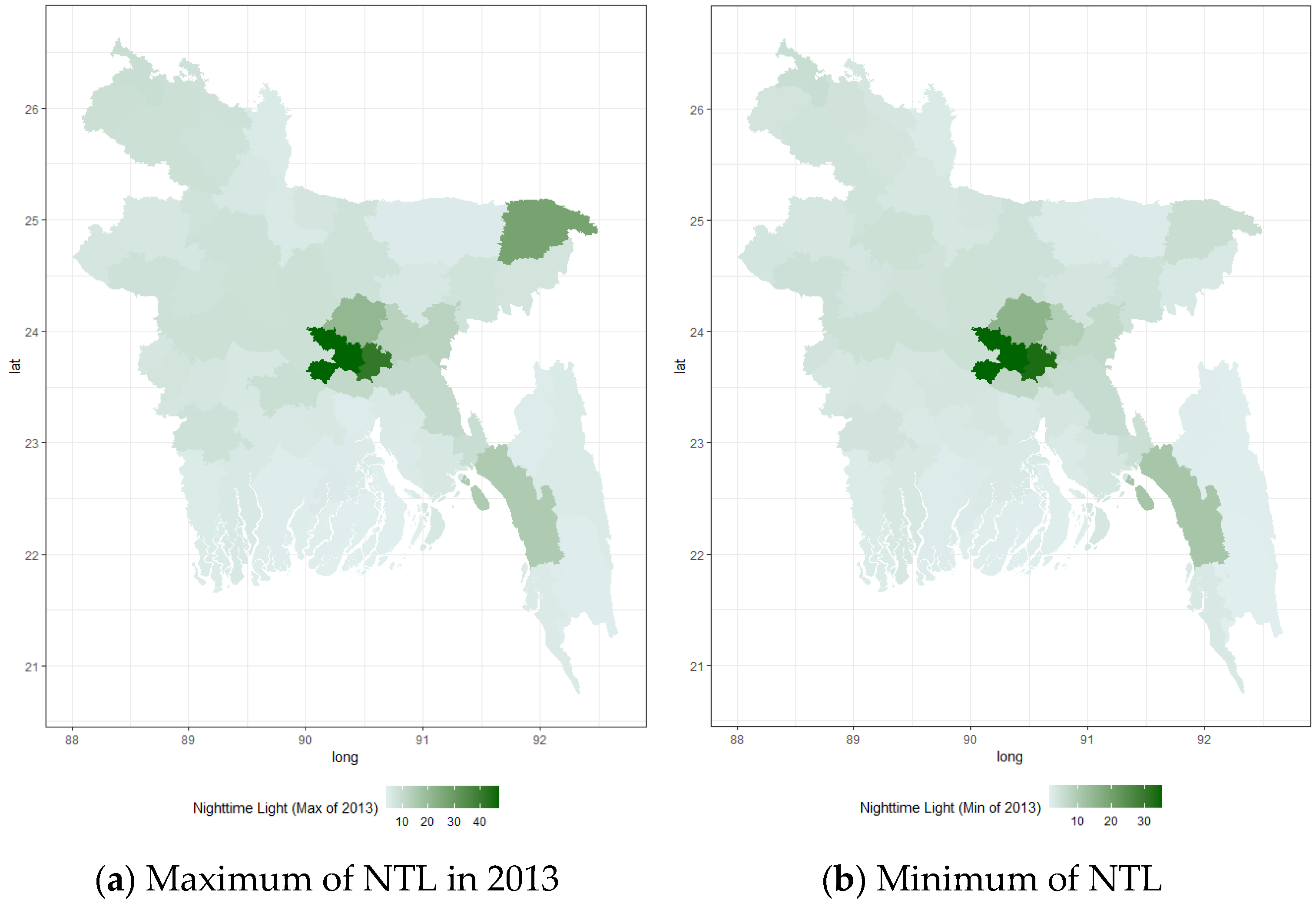
• Nighttime Lights (NTL): Obtained from the Visible Infrared Imaging Radiometer Suite (VIIRS) and, historically, from DMSP-OLS archives. These data are available at relatively high frequency (monthly composites or better) and provide a proxy for overall economic intensity.
• Enhanced Vegetation Index (EVI): Derived from Landsat imagery and updated biweekly or monthly, EVI tracks vegetation cover changes that can correspond to shifts in agricultural or other land-use activities.

By linking satellite image pixels to the administrative boundaries of each district, we computed aggregated measures of NTL and EVI intensity per district and their intra-year volatility (standard deviations). As Keola et al. (2015) [11] and others indicated, coupling NTL with land-cover or vegetation data can yield more robust approximations of local economic conditions, particularly in rural or partially urbanized areas.

2.2.1. Nighttime Lights (NTL)

NTL values represent the radiance detected in the visible band during evening overpasses. While these values are generally stable, certain anomalies—resulting from natural phenomena such as lightning or localized measurement errors—can create outliers in monthly or weekly composites. Rather than discarding these anomalies outright, we occasionally track them as potential indicators of unusual local events. For annualized analysis, we typically average the monthly readings; however, we retain higher-resolution data for mixed-frequency approaches (Section 3) to capture seasonality or short-term disruptions.

2.2.2. Enhanced Vegetation Index (EVI)

The EVI is particularly relevant for regions undergoing transitions from agriculture to nonagricultural sectors, as it reflects plant health and canopy density. In heavily urbanized districts, EVI fluctuations may be minimal, in contrast with districts undergoing deforestation or expanding built-up areas. The EVI can provide early signs of structural changes in land use. Thus, we incorporate the EVI means and volatility over monthly or quarterly windows to detect rapid adjustments in agricultural or periurban zones.

We extracted the NTLs from the VIIRS (VIIRS collects visible and infrared images and global observations of the land, atmosphere, cryosphere, and oceans) archive, which is available from 1992 and the EVI using Landsat data. Although we extracted the remote sensing data from VIIRS and Landsat, there are other sources for obtaining the data.

Table 1. Possible application of satellite image.

Source	Economics Applications	Highest Resolution	Pricing	Availability by Years	Examples	Address
Landsat	Urban land cover, beaches, forest cover, mineral deposits	30 m	Free	1972—(8 satellites)	[12,13]	https://goo.gl/Xhqya5, accessed on 16 March 2025
MODIS	Airborne pollution, fish abundance	250 m	Free	1999—(Terra); 2002—(Aqua)	[1,14]	https://goo.gl/NhHU6x, accessed on 16 March 2025
Night lights (DMSP-OLS, VIIRS)	Income, electricity use	~1 km	Free digital annual (DMSP-OLS) and monthly (VIIRS) composites	Digital archive 1992–2013+ (VIIRS 2012–; film archive 1972–1991)	[2,3]	https://goo.gl/vdIksu, accessed on 16 March 2025
SRTM	Elevation, terrain roughness	30 m	Free	2000 (static)	Ref. [15] via Global AgroEcological Zones (GAEZ) data	https://goo.gl/6zKR4x, accessed on 16 March 2025
DigitalGlobe (including Quickbird, Ikonos)	Urban land cover, forests	<1 m	Not free	1999—(6 satellites)	[16,17]	https://goo.gl/0rL1nW, accessed on 16 March 2025

Source: Donaldson and Storeygard (2016) [18].

presents the data sources we considered in an earlier version of this draft

The DMSP (Defense Meteorological Satellite Program) has been operated by the U.S. Air Force since the 1970s to detect the visible and near-infrared (VNIR) emissions from cities and towns. The DMSP-OLS (Operational Linescan System) is a system for acquiring global daytime and nighttime imagery of the Earth. According to Table 1, DMSP-OLS and VIIRS are available sources. DMSP’s satellites overpass at local time in the 7 p.m. to 9 p.m. range in each region, and they collect nighttime lights, which are defined as a class of derived products of the low-light imaging data in spectral bands, where electric light emissions are observed. According to Hu and Yao (2019) [19], VIIRS nighttime lights have several advantages compared to DMSP/OLS, including greater radiometric accuracy, finer geographical resolution, etc., though the satellite’s overpass time is after midnight, when outdoor lights are arguably less related to residential economic activity than DMSP/OLS nighttime lights. Each pixel of the DMSP-OLS nighttime light images is a 30 arc-second grid. It is associated with a numerical value of radiance from 0 to 63 that increases with brightness.

For the map of Bangladesh, the Database of Global Administrative Areas (known as GADM) provides administrative shape files for all sub-areas in Bangladesh. For each area in each year, we clip the nighttime lights map down to the area borders and sum up the numerical values of the radiance of all pixels within their borders.

2.3. Macroeconomic Control Variables

In addition to the remote sensing metrics, we incorporate macro-level indicators published by the BBS and international sources (e.g., the IMF, World Bank) where available. Notable examples include the following:

• Gross Domestic Product (GDP): Annual aggregates, occasionally extrapolated or back-casted for earlier years.
• Industrial Production Index: Typically reported quarterly, reflecting trends in manufacturing output.
• Property Rental Index, Wage Rate Index: When data are disaggregated by district or urban/rural area, we utilize them to enhance the interpolation of missing labor figures.
• CPI, Inflation, and Compensation of Employees: Annual or quarterly measures that proxy macroeconomic climate and wage conditions.

These established macroeconomic variables may, in certain contexts, overshadow remote sensing indicators (e.g., a nationwide increase in GDP may obscure local heterogeneity). Nevertheless, they remain essential for monitoring overall economic trends and calibrating the out-of-sample forecasts (see Section 4 for model comparisons, including ARIMA as a benchmark).

Table 2. List of variables.

Dependent	Explanatory		Sources
Employment (From the survey)	Remote Sensing data	Daily - Night Time Lights (NTL) Biweekly - Enhanced Vegetation Index (EVI)	- VIIRS - Landsat
	From the survey (as control variables)	- Employment-to-population ratio - Employment total - Labor force participation rate	- Labor Force Survey (2005-06, 2013, 2015-16)
	Formal data (as control variables)	Annual - GDP (real, 2015 prices) - GDP per Capita (in USD, real) - Consumer Price Index - Expenditure - Compensation of Employees Quarterly - Industrial Production Index - Property Rental Index Monthly - Avg Daily Wage - Building Construction Cost Index - Consumer Price Index: National - Electricity Generation - Electricity Sales Value/Volume - Wage Rate Index	- Bangladesh Bureau of Statistics

presents the variables considered in this study, including control variables. Formal data, such as GDP, GDP per capita, CPI (inflation), expenditure, and employee compensation, are available annually. Although the GDP-related series are available from 1974, the CPI is collected from 2006. The industrial production and the property rental indices are reported quarterly, from the first quarter of 2005. Data on daily wages, building construction costs, electricity generation, and wage rate are collected monthly. Daily wage and electricity data are available from January 2000, whereas data for the other indicators have been recorded since 2007. Wage rate data are collected at the provincial level, and average daily wage data are obtained from 23 districts classified as “urban” areas. These district-level variables are essential for interpolating employment data from the survey. As we previously discussed, because the LFS was conducted occasionally, we must interpolate those variables to construct the forecasting model. The selected series from the survey, the employment-to-population ratio, total employment, and labor force participation rate were provided in 64 districts; however, many of the observations are missing. The interpolation strategy is introduced in the next section.

2.4. Data Assembly and Preprocessing

• District Boundaries: We used shape files from the GADM to align the remote sensing grids with the administrative districts. This step is critical for ensuring consistency between the LFS-based data (originally categorized by district) and the satellite-based measures (which need pixel-level clipping or summation).
• Time Alignment: LFS data points exist only for specific years (2005–2006, 2013, 2015–2016), while remote sensing and macroeconomic series are available at monthly or quarterly intervals. Consequently, each dataset must be resampled or aggregated carefully to create consistent time series for annual, quarterly, or monthly analyses.
• Outlier Detection and Cleaning: Outliers in NTL data outliers (e.g., from ephemeral lighting or sensor drift) and EVI data (e.g., cloud cover misclassification) are flagged and treated cautiously. Consistent with our sustainability emphasis, extreme variations might indicate localized shocks, such as floods, droughts, or industrial booms rather than a measurement error.
• Interpolation: Due to the sparsity of LFS data, we employ interpolation methods [9] in conjunction with ILO-estimated labor figures, wage indices, and other auxiliary series. This procedure yields more frequent estimates (annual or quarterly) of district-level employment rates, distinguishing between “decent” and “non-decent” jobs. Section 3.3 discusses this in detail.

From the Labor Force Survey in 2016, we derived employment status, as shown in

Table 3. Employment by status and industry in 2016 survey.

Employment Status	Agriculture	Industry	Service	Not Specified	Total
1 [Employer (Self-employed with paid employee)]	612,116	310,375	750,686	7565	1,680,742
2 [Self—employed]	11,727,356	2,008,217	11,614,597	72,823	25,422,993
3 [Contributing family member]	7,278,337	280,103	926,659	16,313	8,501,412
4 [Paid Employee]	265,633	5,892,673	7,169,274	56,904	13,384,483
5 [Day laborer]	4,489,995	4,253,450	1,494,065	9888	10,247,398
6 [Apprentices/intern/trainees (If paid)]	—	26,270	41,224	134	67,628
7 [Domestic worker]	13,146	36,483	503,511	2074	555,214
9 [Others (Specify)]	58,732	87,234	129,928	1759	277,653
Subtotal	24,445,315	12,894,805	22,629,944	167,459	60,137,523
Not employed(including Not in Labor Force)	—	—	—	98,345,011	120,275,046

. As expected, the share of agriculture is high, considering the dropping rate of the agriculture share in other developing countries in Asia. According to the World Bank, for agriculture, forestry, and fishing, value added (% of GDP), East Asia and the Pacific are dropping gradually. Without high-income countries such as Korea, Japan, and Singapore, the rate was 14.4% in 2000 but dropped to 10.3% in 2010 and 8.3% in 2020.

In this sense, we focus on the quality of employment considering the density of population and employment by district and the nighttime light, as explained. Among employment status, we select “employer”, “self-employed(non-agriculture)”, “employee” as a decent job in the sense that we expect that those factors could guarantee a regular salary. We count the share of this job status out of total population of those over age 15. Figure 3 depicts the quality of employment following the above criteria. In both panels, as the color becomes richer, the ratio of decent jobs increases. As we expected, Dhaka and Chittagong, which include more urban area, have more decent jobs, but the rural areas have higher non-decent job levels.

Figure 4 depicts nighttime light during 2013. We collect nighttime light daily by removing noise and then converting to a weekly average. This figure shows the mean and the standard deviation of nighttime lights from this weekly average. As we expected, the means of lights are strong in urban areas, such as Dhaka and Chittagong. Sylhet district shows strong standard deviation in 2013; however, this is due to one outlier in February 2013. Excluding that exception, the standard deviation of this district dropped to a level similar to that of neighborhood districts. We can see a similar pattern in Panel (a) of Figure 3 and Figure 4, respectively.

Although there are high deviations in one district, typically, there is no significant fluctuation over a year. Figure 3, Figure 4 and Figure 5 depict the maximum and minimum nighttime lights during 2013. This type of outlier may be due to lightning or volcanic activity. Instead of removing the outlier, this kind of high volatility is used to track climate disasters or abnormalities. As shown, the distribution of lights is consistent across districts, with the exception of one district. Figure 6 illustrates the monthly average of night lights by district from 2010 to 2021. The monthly average is calculated as the mean of the weekly value based on the calendar date.

2.5. Linking Data to Sustainability Goals

Given the relevance of labor statistics to SDG 8 (Decent Work and Economic Growth), high-frequency data from satellite imagery help pinpoint district-level changes that annual macro aggregates might obscure. For instance, a district undergoing rapid industrialization may show a spike in nighttime lights that precedes the formal reporting of increased manufacturing employment. Promptly detecting such trends supports sustainable policy measures: local governments can develop tailored skill-training programs or invest in infrastructure enhancements to foster inclusive growth.

3. Model

3.1. MIDAS Framework

To predict Bangladesh’s employment, we follow the baseline setup of [19]. Let $y_{i,t}^{*}$ denote the true real GDP per capita in logarithm for country $i$ in year $t$. It is measured as $y_{i,t}$ with error. Let $s_{i,t}$ stand for the statistical capacity of country $i$ in year $t$. Let $z_{i,t}$ denote nighttime lights per capital in the logarithm. It is related to the true real GDP per capita but also contains a measurement error. Let $l_i$ stand for the latitude of the country. We assume that the reported GDP contains an additive measurement error, whose distribution may vary with a different statistical capacity as follows:

$$y_{i,t}=y_{i,t}^{*}+{\epsilon }_{i,t}^y(s_{i,t})$$

(1)

Meanwhile, the nighttime lights are related to the true latent GDP through an unknown production function $m\left(\cdot \right)$ and an additive error term:

$$z_{i,t}=m\left(y_{i,t}^{*}\right)+{\epsilon }_{i,t}^z\left(l_i\right)$$

(2)

The distribution of this error term also varies with the geographical locations.

This setup is not appropriate to nowcast macro variables directly because, if we follow [19], more frequent nighttime lights should be aggregated as an annual one or make an annual average. Using the monthly frequency property of satellite images, we nowcast the target variable such as GDP on a monthly basis of country A, which is categorized as a ‘low’-statistical-capacity country by the World Bank (World Bank, Bulletin Board on Statistical Capacity (https://bbsc.worldbank.org, accessed on 16 March 2025)). In this sense, we nowcast GDP using MIDAS (MIxed DAta Sampling), which enables us to estimate long-frequency variables with short-frequency explanatory variables. Specifically, let $x_{t_m}$ be sampled $m$ times faster, if it is sampled monthly, $m=12$ with annual data, in which case the basic MIDAS model for forecasting $h_q$ a quarter ahead can be described as

$$y_{t_a+h_a}={\beta }_0+{\beta }_{1}B\left(L^{\frac{1}{m}},\theta \right){\widehat{x}}_{t_m}^{\left(12\right)}+{\epsilon }_{t_a}$$

(3)

where

$$B\left(L^{\frac{1}{m}},\theta \right)=\sum _{j=0}^{j^{\max }}b\left(j,\theta \right)L^{\frac{j}{m}}$$

is the exponential Almon lag, where

$$b\left(j,\theta \right)=\frac{\exp ({\theta }_{1}j+{\theta }_2{j}^2)}{{\sum }_{\mathrm{j}=0}^{{\mathrm{j}}^{\max }}\exp ({\theta }_{1}j+{\theta }_2{j}^2)}$$

${\widehat{x}}_{t_m}^{\left(3\right)}$ is skip sampled from the monthly variable, ${\widehat{x}}_{t_m}$. It is proposed by [10] to enable forecasters to include various indicators in a single model.

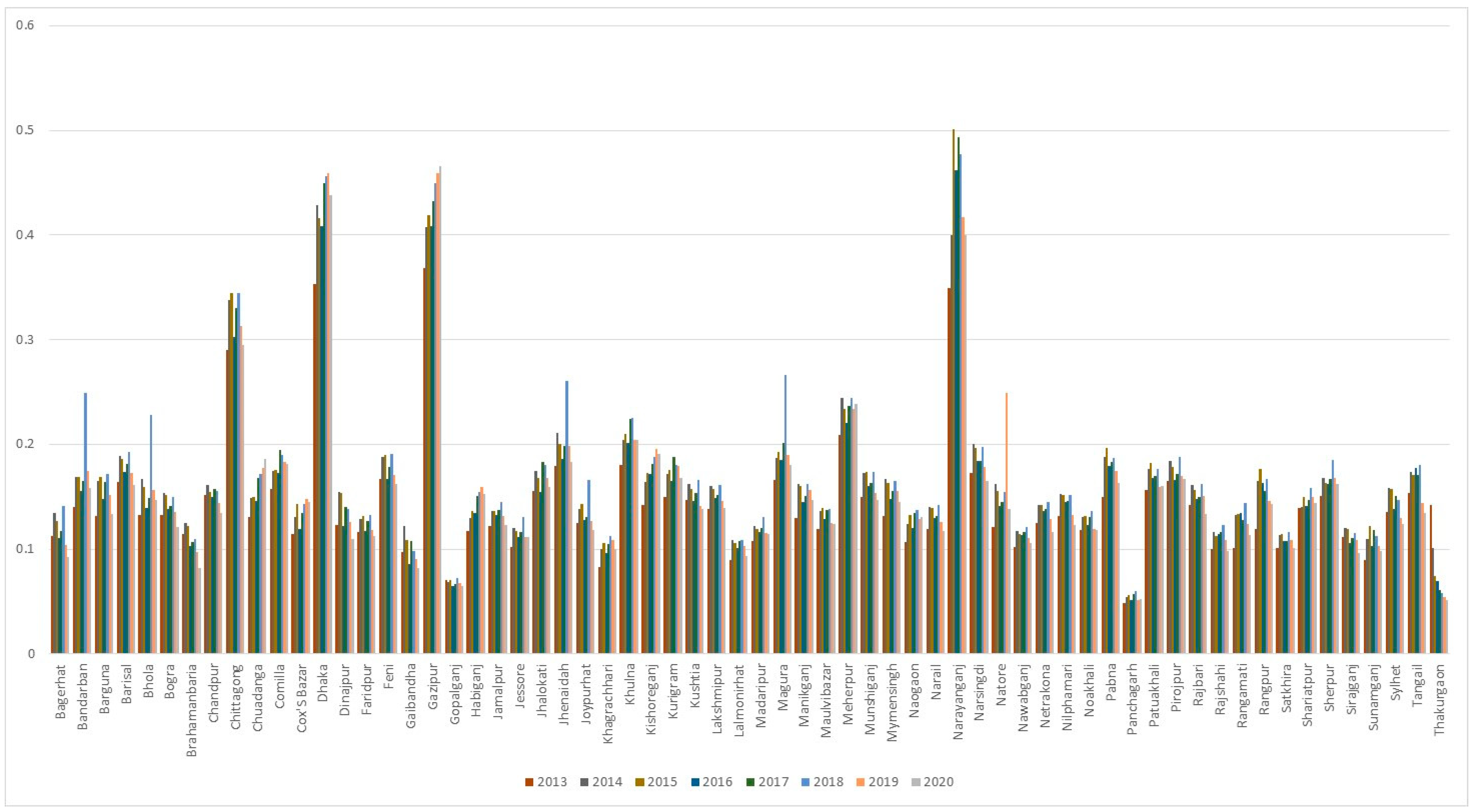
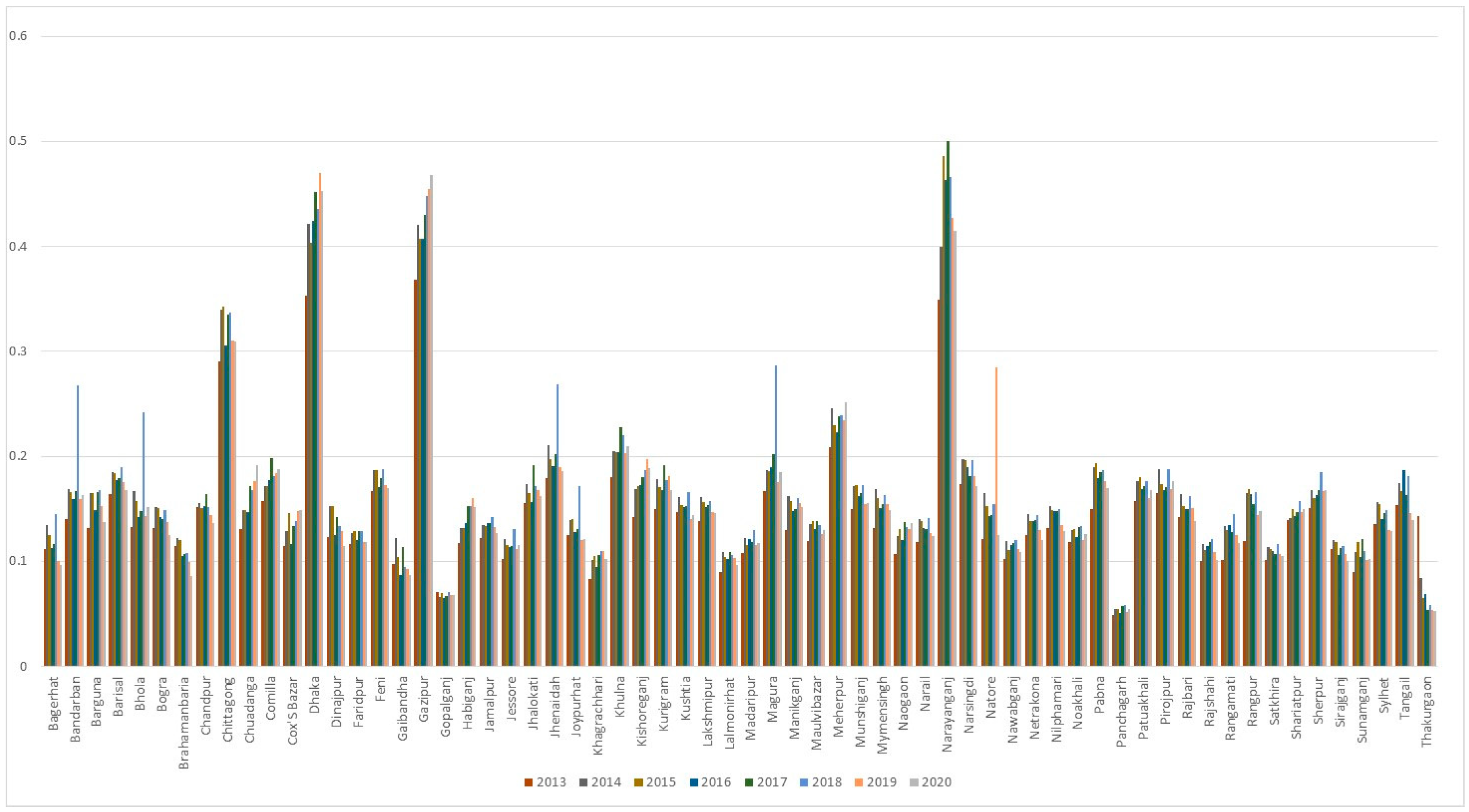
3.2. Target Variable

Here, we specify our target variables in the forecasting model as employment status, $y_t$, defined as a decent job status against total employment. Our principal outcome variable is a district-level measure of “decent” employment, constructed using the LFS classifications:

• Employer (self-employed with paid employees)
• Self-employed (non-agriculture)
• Paid employee (non-agriculture)

We group these job statuses under the umbrella of “decent work”, as they are typically more stable and better remunerated than agricultural jobs or informal/day labor. Following the ILO guidelines and consistent with the BBS categorization, we exclude agricultural day laborers, contributing family workers, domestic workers, and apprentices from our “decent” share. This categorization aligns with SDG 8’s emphasis on quality employment and also accommodates the structure of the Bangladesh labor force data.

Mathematically, let $D_{i,t}$ be the count of individuals in “decent” categories in district $i$ at time $t$, and $P_{i,t}$ the total working-age population, defined as follows:

$$DecentShar{e}_{i,t}={\displaystyle \frac{D_{i,t}}{P_{i,t}}}$$

We similarly define a complementary metric of non-decent work, though our models focus primarily on explaining and forecasting $DecentShar{e}_{i,t}$. Using the ratio instead of the level series can prevent sample bias resulting from the mean effect. Moreover, nowcasting with remote sensing data is not intended to measure employment but, rather, to capture the employment quality trend by districts over time. This target variable is more appropriate than the employment level itself. Among three survey-based data, we derive the job quality in 2005–2006, 2013, and Q3 2015~Q2 2016. Annual data are available for 2006, 2013, 2015 and 2016; thus, interpolation is necessary to generate an annual frequent series. First, good job quality is measured by the number of employments in ‘employer’, ‘self-employed (non-agriculture)’, ‘employee (non-agriculture)’ among ten job statuses collected from the survey. Other employment statuses, such as self-employed (agriculture), day laborer (both agriculture and non-agriculture), contributing family helper, apprentice and domestic worker, are believed to generate lower salaries than the others. As observed, good-quality jobs are condensed more in urban areas. However, we can assume that as towns become more developed, the quality of employment improves. Accordingly, more nighttime lights and a less enhanced Vegetation Index would be shown in more industrialized areas, which have more good-quality jobs. We need to extend these at least to annual variables. Therefore, the first thing to do is to construct these sparse employment data from the LFS to be annual data. In this regard, we interpolate them using ILO-estimated employment-related variables estimated by ILO, such as employment occupation, employment-to-pop ratio, and labor participation. All these are available from ILO statistics (https://ilostat.ilo.org/about/get-started/, accessed on 16 March 2025).

3.3. Interpolation Strategy

First, we interpolate the quality of job status, which is available only in 2006, 2013, 2015 and 2016 using the following reference variables: employment total (by type), employment-to-population ratio, and labor participation rate. The interpolation method we apply is Chow and Lin (1976) [9], which is used for temporal disaggregation or also known as temporal distribution. Temporal disaggregation is the process of deriving high-frequency data from low-frequency data. In addition to the low-frequency data, the Chow–Lin method also uses indicators on the high-frequency data, which contain the short-term dynamics of the time series under consideration. These indicators are time series that are related to the target time series and, thus, measure a different topic than the time series to be estimated. Accordingly, the indicators or reference variables we use for interpolation include the following three variables, which are available at annual frequency.

1.

Employment-to-population ratio by sex, age and rural/urban areas

This analysis distinguishes between rural and urban areas; therefore, each of the 64 districts must be classified either as a rural or urban area before applying the reference variable for interpolation. However, occupation is not categorized within this series. The rural/urban classification is based on the total NTL level, as rural NTL values may be lower than the urban NTLs. Notably, this classification assigns an entire district as either urban or rural, even though each district comprises rural and urban towns simultaneously. Based on the NTLs, the following 21 districts are classified as urban areas: Dhaka, Chittagong, Gazipur, Narayanganj, Mymensingh, Comilla, Sylhet, Tangail, Dinajpur, Bogra, Pabna, Brahamanbaria, Habiganj, Khulna, Jessore, Naogaon, Rajshahi, Rangamati, Rangpur, Maulvibazar, and Sirajganj. Accordingly, the remaining 45 districts are categorized as rural areas. We then interpolate employment by job status using two types of employment-to-population ratios. Since occupation is not included in the dataset, the same reference variable is used for each job status. Sex and age are not considered for simplicity.

2.

Employment by sex, rural/urban areas and occupation

This variable distinguishes the employment by the following occupation:

• Managers
• Professionals
• Technicians and associate professionals
• Clerical support workers
• Service and sales workers
• Craft and related trades workers
• Plant and machine operators, and assemblers
• Elementary occupations and skilled agricultural, forestry and fishery workers

Although this classification does not align with the job statuses considered, job status must be matched with occupation. Occupations 1–5 are selected as representatives of good jobs, whereas the other occupations are considered low-quality jobs. Employment is then interpolated by job quality using two types of employment by occupation. Gender is not considered in this case.

3.

Labor force participation rate by sex, age and rural/urban areas

The labor force participation rate is also distinguished between rural and urban areas. Therefore, employment quality is interpolated following the strategy applied to the first reference variables. Notably, sex and age are not considered in the interpolation process.

4. Empirical Results

4.1. Forecasting Model

Since employment by job quality is interpolated annually, the model is constructed exclusively with the annual-frequency variable. Namely, we set $y_{it}^j$, where $i$ stands for district (1~64), $t$ is the time (annual, 2010–2020), $j$ is for the job status (1–2), as the annual target variables, and the basic forecasting model can be written as follows:

$$y_{i,t+1}^j=\alpha +\sum {\beta }_{1,n}{x}_{it,n}^j+\sum {\beta }_{2,l}{z}_{t,l}+{\gamma }_{it}{s}_{it}+{\epsilon }_{it}^j$$

(4)

where $x_{it,n}^j$ includes the interpolated variable introduced above, $z_t$ is the set of control variables, and $s_{it}$ includes NTL and EVI. For model simplicity, we convert the available quarterly and monthly variable, which is introduced in Table 2, into an annual one. We use this converted annual variable as the control variable. In constructing variables for the remote sensing data, we use NTL and EVI, but the annual levels of NTL and EVI are quite stable over the years. If there is no significant event, such as a volcano eruption or serious lightning, the annual mean of NTL or EVI does not change much and increases slightly as the economy evolves. However, if there is a significant change in a certain district, the volatility of NTL or EVI shows more visible changes. Therefore, we include the volatility of NTL or EVI over a year; then, we can consider the dynamics of EVI or NTL in our forecasting model. Therefore, we include four series: the mean of annual NTL, mean of annual EVI, volatility of annual NTL, volatility of annual EVI. This model is straightforward and easy to estimate, but we waste the variability in EVI and NTL because we convert it to annual, even though we can use it as daily frequency.

Then, we construct a forecasting model with mixed frequency, namely annual and quarterly, as follows.

$$y_{i,t+1}^j=\alpha +\sum {\beta }_{1,n}{x}_{it,n}^j+\sum {\beta }_{2,l}B\left(L^{\frac{1}{q}},\theta \right)z_{t_q,l}^{\left(4\right)}+\sum {\gamma }_{it}B\left(L^{\frac{1}{q}},\theta \right)s_{i{t}_q}^{\left(4\right)}+{\epsilon }_{it}^j$$

(5)

This model is the MIDAS framework, where $z_{t_q,l}^{\left(4\right)}$ and $s_{i{t}_q}^{\left(4\right)}$ are the quarterly control variables and the remote sensing variables, such as NTL and EVI. Note that the set of control variables in this case excludes the annual variables introduced in Table 2. All monthly variables are aggregated to be quarterly variable and included as control variables. We could consider double mixed frequency, such as using quarterly and monthly series as explanatory variables, but it would be very complicated to estimate the model so we do not consider it. Note that the volatility of NTL and EVI now measures changes in a quarter. This model now captures the seasonality of explanatory variables so that we need to extract the seasonality of variables. But, for simplicity of estimation, we do not consider it in this stage.

The next step in developing the forecasting model is how we exploit the high-frequency remote sensing data. We have to take account of the availability of NTL and EVI. Those can be observed every day, but the quality of remote sensing data is not stable due to clouds. The satellite may not see the terrain correctly so that appropriate modification is necessary to obtain remote sensing data. Therefore, to prevent this kind of measurement error, we have to negotiate between the availability and accuracy of the image. Instead of daily series of remote sensing data, the monthly mean and volatility may precisely reflect the socioeconomic variables since those socioeconomic measures are not changed frequently. So, we consider the following quarterly–monthly-type MIDAS framework.

$$y_{i,t_q+1}^j=\alpha +\sum {\beta }_{2,l}B\left(L^{\frac{1}{m}},\theta \right)z_{t_m,l}^{\left(3\right)}+\sum {\gamma }_{i}B\left(L^{\frac{1}{m}},\theta \right)s_{i{t}_m}^{\left(3\right)}+{\epsilon }_{it}^j$$

(6)

Now, $y_{i,t_q+1}^j$ is a quarterly series of employment by job quality, meaning another interpolation that converts annual series to quarterly series is necessary. As in the case where we interpolate sparse employment from the survey into annual series, the reference variable is needed. What we can use in this step is the variables available on a quarterly basis, that is, the Industrial Production Index (quarterly), but this is not available by district. If we use this one, we have to apply the same reference for all 64 districts, and it causes huge bias. Then, we consider monthly variables as the reference variables. Among them, average daily wage is available for some districts, which could be counted as “urban” areas. Therefore, we convert this monthly variable into a quarterly variable by making it an average. There are many missing values in these data; they are not appropriate for use in monthly frequency. Then, we use this as the reference variable to interpolate our target variable for 24 designated districts (Bandarban, Bangladesh, Barisal, Bogra, Chittagong, Comilla, Dhaka, Dinajpur, Faridpur, Jamalpur, Jessore, Khagrachhari, Khulna, Kishoreganj, Kushtia, Mymensingh, Noakhali, Pabna, Patuakhali, Rajshahi, Rangamati, Rangpur, Sylhet, Tangail) (we select those 24 districts because the NTL of districts are above the median of NTL of all areas for the whole sample period). And, for the rest of the districts, the Industrial Production Index is used for the reference variable. In this model, we use all available monthly variables for $z_{t_m}$, and EVI and NTL are in monthly frequency. That is, the volatility of the two variables represents the volatility in a month. Note that $x_{it,n}^j$ was not included since it was originally an annual series, and it becomes more complicated if we interpolate again with monthly series used in interpolating annual variables. $z_{t_m,l}^{\left(3\right)}$ and $s_{i{t}_m}^{\left(3\right)}$ are the set of monthly variables introduced in Table 2 and the mean and volatility of EVI and NTL in a month.

In summary, we suggest three models for describing the employment quality of Bangladesh. Note that we constructed the annual employment quality by interpolating the sparse employment data from the LFS of Bangladesh. The first one is for the annual employment quality, and explanatory variables are transformed to annual series, including remote sensing data. In the second model, the target is the same, but we change the model into mixed frequency so that the explanatory variables are now a quarterly series. Then, in the third model, we again interpolate the employment quality to make the quarterly series. With this, we construct another mixed-frequency model with monthly series at the end.

4.2. Estimation Result

The estimation of models (4)~(6) is conducted through nonlinear least square (NLS), as explained in the Section 3. With this type of nonlinear model, there is no way to verify the sign of coefficients so that it is customary to see the accuracy of the forecasting by comparing the fitted one and the true observation. However, we do not have enough information about our target variables since we created the series through interpolation. Therefore, it is helpful to see the fitted result and whether it can be explained by our common sense. Figure 7 shows the share of good-quality jobs estimated by district and year. Most of the urban districts or the districts consisting of more urban towns show that the share is more than 30% and has an upward trend. But we can also observe some districts which have a low share and have a downward trend in the share. In Tangail and Narsingdi districts, there are estimated shares, which look like outliers. It seems that in those cases, there were climate phenomena, which cause significant volatility. More analysis is necessary to give a more precise explanation of these outliers.

Entries in this figure represent the share of decent employment, such as employer, regular-paid job, self-employed (non-agri), against total employment. The total number can be calculated, but it needs to be weighted by the survey. But we do not have an appropriate weight for the other years. If we apply the same weight for the rest of the years, it produces serious bias. Therefore, it is better to report the ratio.

As explained, the first model cannot exploit more information from higher-frequency data, so we extended the annual model into the mixed-frequency framework, namely MIDAS. With quarterly explanatory variables, we estimate the model of Equation (5), and Figure 3, Figure 4, Figure 5, Figure 6 and Figure 7 show the in-sample result. This model generates annual employment by job quality, meaning that quarterly fluctuations in the target variable cannot be observed. However, we confirm that this model is more responsive to quarterly movement, such as the standard deviation of the EVI, which represents the quarterly volatility of NTLs. The overall trend of the fitted value of employment by job quality is not much different from the result obtained using Equation (4).

The next step is to develop the target variables for conversion into a quarterly series. Although bias appeared during the interpolation of annual data into a quarterly series, additional information can be extracted from the monthly variables. Figure 8 illustrate estimated quarterly employment by job quality from 2013. Since more quarterly and monthly variables are available through 2021, the estimation is extended accordingly. As expected, there was a temporary decline in employment by job quality during 2020, followed by a rapid recovery. However, urban areas, such as Narayanganz and Dhaka, experienced a more pronounced decline in employment. Notably, the employment conditions in the Thakurgaon district deteriorated over time.

Though we have some annual variables up to 2020 and some quarterly variables up to the fourth quarter of 2020, we have a daily NTL series and biweekly EVI series. To exploit the real-time characteristic of two remote sensing data, we constructed the out-of-sample forecast of the employment with the monthly mean and volatility of NTL and EVI. The rest of the control variables, such as the Industrial Production Index and average daily wage, are projected based on the individual AR (1) model in the framework of Equation (6). Figure 9 show the out-of-sample result with the in-sample result from 2016 for the reader’s convenience. The overall movement of employment in this out-of-sample period moves up. It seems that just after the pandemic spread, Bangladesh recovered relatively quickly so that key control variables such as Industrial Production and Wage Index increased at the end of 2020. As a result, the projected control variables using the AR (1) model also show an upward trend in 2021. But, in 2022, due to the AR model’s mean reversion characteristic, the overall employment by job quality dropped at the end. Therefore, we conclude that the state of the economy affects the overall employment status. However, the result is still worth considering because Figure 10 show which districts offer good job opportunities. Understanding this trend is helpful for policymakers to implement labor policies by district.

5. Conclusions

This study aimed to measure and forecast the labor market status in Bangladesh by integrating remote sensing data and sparse LFS observations. The results highlight the potential of high-frequency satellite indicators—NTLs and the EVI—to capture local economic dynamics, particularly in contexts where official data are infrequent or subject to significant delays. By incorporating MIDAS techniques and interpolation methods (Chow–Lin), we generated annual and quarterly estimates of district-level “decent” employment shares that provide a closer-to-real-time analysis of Bangladesh’s labor markets.

5.1. Key Findings

Feasibility of Remote Sensing for Labor Market Monitoring. Our analysis shows that incorporating remote sensing variables can add explanatory power beyond aggregate macroeconomic indicators alone. NTL, in particular, appears to correlate with regions undergoing industrialization or urbanization, while EVI helps detect changes in agricultural areas. These effects become more evident at higher frequencies, revealing short-term shocks or outlier districts that annual averages might mask.

Value of Mixed-Frequency Models. The MIDAS framework allowed us to combine monthly (remote sensing) and quarterly (macroeconomic) data to estimate district-level employment trends in near-real time. This approach compares favorably with traditional time-series models (e.g., ARIMA), which often rely on a single-frequency structure and, thus, cannot fully exploit fast-arriving satellite data or partial mid-year statistics. Our out-of-sample forecasts through 2022 suggest that remote sensing variables do indeed detect some local idiosyncrasies, though macro indicators like industrial production dominate broad trends in employment.

Utility for Sustainable Development (SDG 8). Frequent updates to local employment estimates can bolster policy responsiveness, a central theme in SDG 8: Decent Work and Economic Growth. The findings highlight how district-level tracking of “decent” employment shares can inform targeted skill training, wage support, and other sustainability-oriented labor policies, thereby enhancing inclusive economic growth. The early detection of localized job market dips (e.g., after a natural disaster or pandemic-related disruption) helps local governments act more effectively to prevent longer-term socioeconomic damage.

5.2. Limitations

Because official labor statistics in Bangladesh are scarce, it is not possible to fully verify all out-of-sample predictions generated by our model. The limited availability of recent LFS data further complicates the validation of our estimates in the short term. Nevertheless, as newer rounds of LFS or other reliable survey data become publicly available, we can cross-check and refine our forecasting results. While integrating remote sensing data provides valuable district-level insights, these effects may be overshadowed by broader macroeconomic trends, such as GDP growth or fluctuations in the Industrial Production Index. In smaller or predominantly rural districts, signals captured by NTLs or the EVI may be masked by stronger national business cycles, making isolating the local drivers of employment changes challenging.

Satellite-derived NTL and EVI data may also contain outliers resulting from cloud cover, weather events, or sensor calibration issues. Although extreme values have been flagged and processed with caution, there remains a risk of conflating genuine economic shocks with anomalous measurement errors. Ensuring data quality is, therefore, a crucial step in leveraging remote sensing for labor market analysis. Our application of the Chow–Lin methodology to bridge gaps in the LFS time series fundamentally depends on the auxiliary reference variables used. District-level wage or employment proxies may sometimes be incomplete or unevenly reported, potentially introducing bias into the interpolated employment estimates. This underscores the importance of maintaining a diverse and robust reference series where possible.

5.3. Directions for Future Research

Satellite-derived thermal data or land surface temperature (LST) measures could refine estimates of agricultural or informal sector activity—an essential consideration for predominantly rural and climate-vulnerable areas of Bangladesh. Further work could employ cluster detection algorithms on NTL and EVI series to categorize districts with similar time-varying labor profiles, as well as identifying outliers that deviate significantly from typical patterns. Such analyses would contribute to a more comprehensive understanding of spatial heterogeneity in local labor markets.

The modeling framework could also be extended to other low- and middle-income countries with limited data infrastructure, provided suitable modifications are made (e.g., adjusting reference variables or recalibrating weighting schemes). Comparing results across multiple national contexts would shed light on how remote sensing signals vary with institutional and geographic differences. Linking local labor market estimates to real policy interventions (e.g., training programs, microfinance initiatives) may strengthen the evidence base for how the early detection of labor shifts can prompt effective action. Evaluating these interventions would help determine whether satellite-informed policy leads to measurably better employment outcomes.

5.4. Concluding Remarks

This research highlights a promising approach for leveraging high-frequency satellite observations to enhance labor market monitoring in data-scarce environments. By bridging persistent information gaps, these mixed-frequency models help public officials and other stakeholders make more timely and spatially targeted decisions, aligning local labor policies more effectively with sustainable development goals. While methodological and data-related limitations persist, the evidence suggests that remote sensing can serve as a practical complement to traditional labor surveys, particularly for rapidly evolving or under-resourced contexts like Bangladesh.

References

1. Burgess, R.; Hansen, M.; Olken, B.A.; Potapov, P.; Sieber, S. The Political Economy of Deforestation in the Tropics. Q. J. Econ. 2012, 127, 1707–1754. [Google Scholar] [CrossRef]
2. Chen, X.; Nordhaus, W.D. Using luminosity data as a proxy for economic statistics. Proc. Natl. Acad. Sci. USA 2011, 108, 8589–8594. [Google Scholar] [PubMed]
3. Henderson, J.V.; Storeygard, A.; Weil, D.N. Measuring Economic Growth from Outer Space. Am. Econ. Rev. 2012, 102, 994–1028. [Google Scholar] [PubMed]
4. Rahman, S.; Mohiuddin, H.; Kafy, A.-A.; Sheel, P.K.; Di, L. Classification of cities in Bangladesh based on remote sensing derived spatial characteristics. J. Urban Manag. 2019, 8, 206–224. [Google Scholar]
5. Wahed, M.; Rizvee, R.A.; Haque, R.R.; Ali, A.M.; Zaber, M.; Ali, A.A. What Can Nighttime Lights Tell Us about Bangladesh? In Proceedings of the 2020 IEEE Region 10 Symposium (TENSYMP), Dhaka, Bangladesh, 5–7 June 2020; pp. 1612–1615. [Google Scholar]
6. Bangladesh Bureau of Statistics. Labor Force Survey 2005–2006; The Bangladesh Bureau of Statistics: Dhaka, Bangladesh, 2006.
7. Bangladesh Bureau of Statistics. Labor Force Survey 2013; The Bangladesh Bureau of Statistics: Dhaka, Bangladesh, 2013.
8. Bangladesh Bureau of Statistics. Labor Force Survey 2015–2016; The Bangladesh Bureau of Statistics: Dhaka, Bangladesh, 2016.
9. Chow, G.C.; Lin, A.-L. Best Linear Unbiased Estimation of Missing Observations in an Economic Time Series. J. Am. Stat. Assoc. 1976, 71, 719–721. [Google Scholar]
10. Ghysels, E.; Santa-Clara, P.; Valkanov, R. The midas touch: Mixed data sampling regression models. In CIRANO Working Papers, 2004s-20; CIRANO: Barcelona, Spain, 2004. [Google Scholar]
11. Keola, S.; Andersson, M.; Hall, O. Monitoring Economic Development from Space: Using Nighttime Light and Land Cover Data to Measure Economic Growth. World Dev. 2015, 66, 322–334. [Google Scholar]
12. Faber, B.; Gaubert, C. Tourism and Economic Development: Evidence from Mexico’s Coastline. Am. Econ. Rev. 2016, 109, 2245–2293. [Google Scholar] [CrossRef]
13. Foster, A.D.; Rosenzweig, M.R. Economic Growth and the Rise of Forests. Q. J. Econ. 2003, 118, 601–637. [Google Scholar] [CrossRef]
14. Foster, A.; Gutierrez, E.; Kumar, N. Voluntary Compliance, Pollution Levels, and Infant Mortality in Mexico. Am. Econ. Rev. 2009, 99, 191–197. [Google Scholar] [PubMed]
15. Costinot, A.; Donaldson, D.; Smith, C. Evolving Comparative Advantage and the Impact of Climate Change in Agricultural Markets: Evidence from 1.7 Million Fields Around the World. J. Political Econ. 2016, 124, 205–248. [Google Scholar]
16. Jayachandran, S.; de Laat, J.; Lambin, E.F.; Stanton, C.Y. Cash for Carbon: A Randomized Controlled Trial of Payments for Ecosystem Services to Reduce Deforestation; Northwestern University: Evanston, IL, USA, 2016. [Google Scholar]
17. Marx, B.; Stoker, T.M.; Suri, T. There is No Free House: Ethnic Patronage in a Kenyan Slum. Am. Econ. J. Appl. Econ. 2015, 11, 36–70. Available online: http://www.mit.edu/~tavneet/Marx_Stoker_Suri.pdf (accessed on 16 March 2025). [CrossRef]
18. Donaldson, D.; Storeygard, A. The View from Above: Applications of Satellite Data in Economics. J. Econ. Perspect. 2016, 30, 171–198. [Google Scholar] [CrossRef]
19. Hu, Y.; Yao, J. Illuminating Economic Growth. In IMF Working Paper WP/19/77; International Monetary Fund: Washington, DC, USA, 2019. [Google Scholar]
Figure 1. Total employment by district or division (2013 and 2016 (Q2)). Note: The figure is drawn by the author.
Sustainability 17 02807 g001
Figure 2. Bangladesh population ((a) 2011 and (b) 2021).
Sustainability 17 02807 g002
Figure 3. Quality of employment in 2013.
Sustainability 17 02807 g003
Figure 4. Nighttime light during 2013.
Sustainability 17 02807 g004
Figure 5. Change in nighttime light during 2013.
Sustainability 17 02807 g005
Figure 6. Time series of nighttime light by districts.
Sustainability 17 02807 g006
Figure 7. The share of good-quality job employment by district and year (estimated by Equation (4)).
Sustainability 17 02807 g007
Figure 8. The share of good-quality job employment by district and year (estimated by Equation (5)).
Sustainability 17 02807 g008
Figure 9. The share of good-quality job employment by district and quarter (estimated by Equation (6)).
Sustainability 17 02807 g009
Figure 10. Out-of-sample forecast of the share of good-quality job employment.
Sustainability 17 02807 g010