Assessing Rural Habitat Suitability in Anhui Province: A Socio-Economic and Environmental Perspective

Abstract

Assessing rural habitat suitability and its connection to land response is a vital tool for understanding the socio-economic and environmental challenges in rural areas tailored to local contexts. This study fills existing research gaps by examining the suitability of rural habitats in Anhui Province, opening pathways to reveal how rural sustainability may connect to land. Using the autoregressive distributed lag (ARDL) model, it analyzes the short- and long-term effects of socio-economic and environmental factors on rural suitability across various counties. Additionally, a descriptive analysis explores the pathways linking rural suitability to land use responses. The findings reveal that rural greening, village planning, and housing area per resident positively influence rural habitat suitability in both the short and long term. However, agricultural income growth shows a negative impact, potentially due to structural issues in the sector. Environmental factors like temperature and rainfall have a limited influence on rural suitability. The study underscores the importance of suitable rural infrastructure, namely enhancing rural greening rate, implementing village plans, and improving housing for sustainable rural development. Regional variations in rural habitat suitability across Anhui Province are also evident. While some cities, such as Huaibei and Anqing, demonstrate success in revitalization, others, like Suzhou and Chizhou, face challenges. The results highlight the need for region-specific strategies that account for local environmental, economic, and infrastructural contexts. Tailored approaches are essential to achieving long-term, effective rural development in the province.

1. Introduction

Land is essential to the prosperity of human civilizations, influenced by the complex interplay of natural processes, socio-economic factors, and environmental sustainability. Rural development and restructuring play a crucial role in achieving optimal spatial adjustments for regional revitalization [1]. Rural areas form the foundation of socio-economic development, and their sustainable growth is vital for urban–rural integration and habitat suitability strategies. In light of global economic shifts and growing ecological concerns, balancing economic growth, social welfare, and natural resource protection in rural areas has become a pressing issue for both scholars and policymakers [2]. With socio-economic changes making rural areas more vulnerable, accurate and quantitative assessments of rural development are essential for shaping effective rural development strategies [3,4].

Rural decline has emerged as a global challenge that threatens the prospects for sustainable development [5]. Achieving sustainable rural development is complex and requires careful balancing of economic growth, environmental protection, and social welfare improvements [6]. In response, the United Nations adopted the 2030 Agenda for Sustainable Development in 2015, which outlines 17 Sustainable Development Goals (SDGs) to guide global socio-economic progress [7]. In essence, this agenda emphasizes the importance of “Sustainable Cities and Human Settlements,” urging nations to harmonize economic growth with environmental conservation for a more equitable and resilient future.

This goal is particularly crucial in rural development, as rural areas are not only vital for food production and ecosystem preservation but also serve as key regions for poverty eradication and advancing social equity. However, rural livelihoods are increasingly threatened by climate change and social vulnerability, necessitating agricultural adaptation strategies and targeted policy interventions to promote sustainable development [8]. Additionally, the efficiency of resource allocation in agriculture significantly boosts rural residents’ life satisfaction and economic welfare, with farmers’ income primarily derived from agricultural production [9,10]. Addressing these challenges requires integrated approaches that support both environmental sustainability and socio-economic resilience.

Rural habitat suitability is essentially the reconstruction and upgrading of rural society, economic forms, and ecology [11]. In China, the rural habitat suitability strategy has driven policy changes to assess the suitability of rural living conditions [2,12]. This strategy emphasizes not only the modernization of the rural economy but also the enhancement of ecological protection, cultural heritage, and governance capacity. The Chinese government launched a three-year action plan in 2018, followed by a five-year campaign in 2021, to enhance the rural living environment, aiming to improve rural residents’ quality of life and promote sustainable rural development [13]. Rural transformation involves changes in farming practices, land use, and sectoral interactions [14], where improving greening rates, infrastructure, and agricultural modernization, alongside ecological protection, are key to sustainable development.

In recent decades, the world has made remarkable achievements in rural development [15]. However, research in rural development, particularly in Anhui Province, still has significant gaps. Current studies focus on differentiating rural functions—agricultural, non-agricultural, and ecological—proposing evaluation systems for rural habitat coordination and analyzing human settlement evolution and vulnerability using GIS [16,17,18]. Despite these efforts, there is a need for further comprehensive exploration of rural dynamics. Analyzing rural habitat suitability can provide valuable insights into changes in rural characteristics and land use responses, helping to understand how socio-economic factors and environmental conditions influence land utilization and habitat viability. In essence, there is still a lack of systematic assessment of the interactions between socio-economic and environmental factors, leading to an insufficient understanding of both short- and long-term impacts across various scales, as well as an incomplete exploration of the heterogeneity in regional development paths.

Therefore, to address existing research gaps and gain a deeper understanding of the challenges faced by rural areas and their land use responses, this study focuses on Anhui Province as a case study. Using the autoregressive distributed lag (ARDL) model, it explores both short-term and long-term dynamic effects of socio-economic and environmental factors on rural suitability, examining these issues across different counties. Then, a descriptive analysis will be performed to unlock the close link between rural features and land use response. By analyzing the complex interactions between these factors, the research contributes to the ongoing debate, providing a more comprehensive and consistent understanding of the challenges in rural areas.

2. Research Framework and Theoretical Basic

Interest in the direct interactions between individuals and nature has grown rapidly, highlighting the deeply interconnected relationship between humans and the environment [19,20]. Rural areas have become increasingly vulnerable due to socio-economic changes, with population growth having a significant impact on land use patterns over time [3,21,22]. In Anhui Province, sustainable development was not prioritized before 2014, with economic growth taking precedence in decision making. This focus on economic expansion led to the overexploitation of water resources and environmental degradation [23]. As a result, rural areas have faced significant socio-economic and environmental challenges. These challenges highlight the need for a more balanced approach, integrating both economic growth and environmental sustainability to ensure long-term resilience and well-being in rural communities.

Rural habitat suitability is intricately connected to the development of sustainable human habitats [17], which requires addressing both socio-economic and environmental factors. This study utilizes the rural habitat suitability index to assess rural habitat quality. In Anhui Province, achieving sustainable development involves integrating key variables that enhance habitat quality and ensure long-term resilience. While modern agriculture’s use of pesticides boosts productivity and food security, it also poses significant risks to the environment and human health, including soil and water contamination [24,25]. Likewise, the comprehensive utilization rate of livestock and poultry waste plays a vital role in mitigating pollution and enhancing soil fertility, which in turn supports agricultural productivity and environmental sustainability [26,27]. A balanced approach to these issues is critical for rural habitat suitability in Anhui Province.

Greenery is a critical indicator of the health and sustainability of urban ecosystems [28]. So, in the context of this study, greenery refers to the presence and extent of green spaces, vegetation, and forests in rural areas, contributing to environmental quality, biodiversity, and overall habitat suitability. In rural areas, the greening rate plays a key role in enhancing environmental sustainability by improving air quality, supporting biodiversity, and creating more livable spaces. Moreover, understanding the factors that influence the vulnerability of forested areas is essential for both human well-being and effective governance, as it helps manage the balance between ecosystem supply and demand [29,30]. In addition, villages with well-prepared village plans are more likely to achieve organized infrastructure development and efficient resource management. These plans ensure a strategic approach to land use, agricultural practices, and environmental conservation, all of which are critical to building sustainable rural habitats. Together, these factors contribute to the overall resilience and livability of rural communities.

Agricultural land is a crucial resource for both national economic development and rural households [31]. Agricultural productivity, underpinned by robust grain production capacity, plays a vital role in ensuring food security and economic stability, particularly in rural areas, forming the foundation for achieving these goals [32,33]. Consequently, China has reached a critical juncture in advancing rural revitalization [34]. Hence, the connection between rural habitat suitability and land use is becoming increasingly apparent, as effective land use practices have become among the most crucial aspects for optimizing agricultural productivity, supporting rural livelihoods, and ensuring long-term sustainability.

Climatic factors, such as temperature and rainfall, can significantly influence land use [35]. The relationship between land and global climate has been well established over time, with climate conditions shaping the viability and productivity of land for various uses [36,37]. As climate patterns evolve, they can drive changes in land management practices and overall land utilization, highlighting the interconnectedness of environmental and land-use systems. Average temperature and rainfall impact agricultural yields and habitat quality, which is crucial for ecological civilization and socio-economic development [38]. Areas with favorable climatic conditions are more likely to support sustainable farming practices, fostering long-term agricultural productivity. Conversely, extreme weather patterns, such as droughts or excessive rainfall, can exacerbate environmental degradation, negatively impacting crop yields and soil health. Ultimately, the balance between agricultural productivity, environmental health, infrastructure development, and public health is essential for determining the long-term viability of rural areas. This integrated approach is crucial for ensuring that rural communities can thrive and support their populations sustainably.

Rural habitat suitability in Anhui Province demands a balanced approach integrating socio-economic development with environmental sustainability. Rapid economic growth has caused resource overexploitation and environmental degradation, leaving rural areas vulnerable. Key factors such as pesticide use, waste management, sanitation, and village planning are vital for improving environmental health and public well-being. Agricultural productivity, reliant on favorable climate conditions, underpins rural economies. A harmonious balance of agricultural, environmental, and infrastructural development is essential for achieving resilience and sustainable growth in rural Anhui Province.

3. Materials and Methods

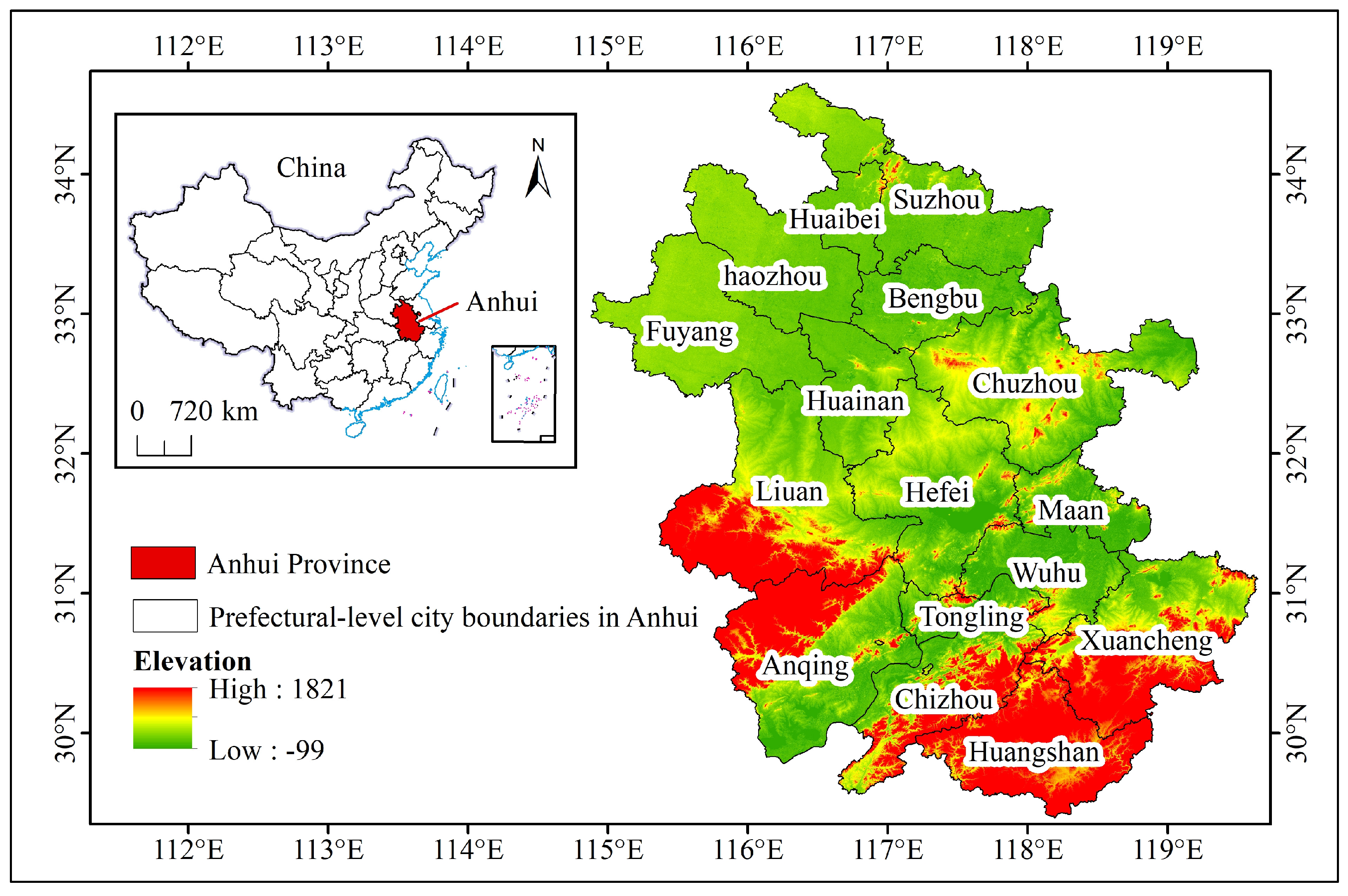
3.1. Study Area

Anhui Province is located between 29°41′ N and 34°38′ N latitude and 114°54′ E and 119°37′ E longitude (Figure 1). It is located in east China, in the middle and lower reaches of the Yangtze River and Huaihe River, as well as the hinterland of the Yangtze River Delta [39]. According to the China Statistical Yearbook 2023, it covers approximately 139,600 square kilometers and has a population of 61 million people. The province’s terrain is characterized by a diverse mix of plains, hills, and mountains, with a topography that slopes from southwest to northeast. Anhui is divided into three natural regions: Northern Anhui (plains), Central Anhui (Central Anhui Hills), and Southern Anhui (Southern Anhui Mountains), and spans the Huai River, Yangtze River, and Xin’an River water systems. As one of China’s major agricultural production bases, Anhui’s land is primarily used for farming, which accounted for 55.38% of the province’s total area in 2020, with the majority of agricultural land located in the plains of Northern and Central Anhui.

3.2. Data Resource

The data for this study were sourced from reputable organizations, including the Anhui Provincial Bureau of Statistics, the Anhui Provincial Department of Ecology and Environment, and the China Statistical Yearbook Provincial Statistical Yearbooks (2001–2020). These datasets offer a comprehensive overview of Anhui’s socio-economic and environmental trends over the past decade.

3.3. Selected Variables and Description

In this study, we first select several primary variables. We then use the variance inflation factor (VIF) to eliminate variables causing multicollinearity. The variance inflation factor (VIF) helps identify multicollinearity in regression models. To begin, prepare the data and fit an initial regression model (See Supplementary Materials). Calculate the VIF for each predictor variable and identify those with a VIF above 5. Remove the variable with the highest VIF, refit the model, and calculate VIF again. Repeat this process, removing variables with high VIFs until all predictors have VIFs of 5 or less. Finally, validate the model’s fit, significance, and interpretability. This iterative approach ensures a robust and meaningful regression model free of multicollinearity. The final variables to be used in the model are presented in

Table 1. Description of the selected variables.

Variable	Mean	Std. Dev.	Min	Max
Rural habitat suitability (Indice)	0.221	0.049	0.128	0.331
Rural greening rate (%)	5.523	1.385	2.647	8.965
Village plans (%)	7.698	1.848	4.281	12.372
Temperature (average °C)	16.059	1.594	10.889	23.055
Rainfall (average mm)	0.003	0.001	0.002	0.007
Income of farmers (growth rate%)	34.462	1.443	30.132	37.199
Living space (square meters)	7.715	1.82	4.123	12.829

.

The descriptive statistics of the variables reveal important insights into the socio-economic and environmental conditions of rural areas. For rural habitat suitability, the index has a mean value of 0.221, which indicates a moderate income level across the regions. Interestingly, the low standard deviation (0.049) suggests that the variability in income is minimal, with values ranging from 0.128 to 0.331. Moreover, when examining environmental factors such as the rural greening rate, the average rural greening rate is 5.523, accompanied by a moderate variability as shown by a standard deviation of 1.385. This variability becomes more evident when we consider that some areas have significantly lower greening efforts (2.647) compared to others (8.965).

In addition, the data on village plans highlight that, on average, 7.698% of villages have implemented planning initiatives. While this indicates progress, the range (4.281 to 12.372) points to considerable differences between regions, which could stem from varying levels of local development priorities. Meanwhile, climatic factors such as temperature and rain show less variability. For instance, the average temperature is 16.059 °C, with a narrow range of 10.889 °C to 23.055 °C, suggesting relatively stable climatic conditions. Similarly, rainfall exhibits low variability, with an average of 0.003 m and a range of 0.002 to 0.007 m, which reflects consistent but low precipitation levels across the study area.

Turning to economic indicators, the income of farmers, the growth rate of farmers’ income presents an average of 34.462% during the study period, with moderate variability (standard deviation of 1.443) and a range of 30.132 to 37.199%. This shows that while many regions are experiencing growth, some outperform others significantly. Lastly, the analysis of housing conditions, as indicated by living space, reveals an average housing area of 7.715 square meters per rural resident. However, the wide range (4.123 to 12.829 square meters) and moderate standard deviation (1.82) underscore disparities in living conditions.

In summary, the descriptive statistics provide a comprehensive overview of the studied variables. While some indicators, such as temperature and rainfall, display little variability, others, like housing area and greening rates, highlight significant regional disparities. These findings underscore the need for tailored interventions to address the unique challenges and opportunities within different rural areas.

3.4. Method

Motivation for Model Choice

The autoregressive distributed lag (ARDL) approach was selected for its ability to manage variables with mixed integration orders, I(0) and I(1), which are common in socio-economic and environmental panel data. It is particularly suitable for studying rural habitat suitability in Anhui Province, where some variables are stationary at the level, and others require differencing. ARDL is also efficient in small sample sizes and does not require all variables to be integrated in the same order, unlike methods such as VECM [40]. This flexibility is essential due to the varied nature of factors like income, education, environmental quality, and rural infrastructure influencing rural habitat suitability. The ARDL methodology is ideal for examining short- and long-term dynamics of the suitability of rural habitats in Anhui Province. Utilizing the PMG, MG, and DFE models allows for town-specific effects while generalizing long-term relationships. Cointegration tests, Granger causality, and the Hausman test ensure the robustness and accuracy of the findings.

In sum, existing research on rural development in Anhui Province mainly focuses on rural function differentiation, habitat coordination, and GIS-based analysis of settlement evolution and vulnerability. However, there is a lack of systematic assessment of socio-economic and environmental interactions, limiting understanding of their short- and long-term impacts. This study applies the ARDL model to explore these factors’ effects on rural habitat suitability, offering comprehensive insights into dynamic interactions and regional heterogeneity for sustainable development.

Order of Integration: To ensure the correct application of the ARDL model, panel unit root tests were performed to identify the integration order of the variables. The tests applied included the Levin, Lin, and Chu (2002) test, as well as the Maddala and Wu (1999) test, which help assess stationarity across the panel data [41,42]. If the variables are found to be I(0) or I(1), the ARDL approach is suitable. However, if any variable is found to be I(2), the ARDL approach is not appropriate.

Model Specification: The ARDL model for each township in Anhui Province can be written as:

$$y_{it}={\alpha }_i+\sum _{k=1}^p{\lambda }_{i,k}{y}_{i,t-k}+\sum _{j=1}^q{\beta }_{i,j}{X}_{i,t-j}+{\gamma }_i{z}_{i,t}+{\mu }_i+{ϵ}_{i,t}$$

where y_it represents the dependent variable (rural habitat suitability) for county i at time t; X_(i,t−j) represents a set of independent variables (income, environmental quality, etc.) for county i at time t − j; and λ_(i,k) captures short-run dynamics, while γ_i captures the long-run relationship; μ_i is a county-specific fixed effect capturing unobserved heterogeneity across counties; z _i,t represents county-specific control variables included to account for other potential influences on rural habitat suitability; ϵ_it is the error term; The indices i and t range over the following values: i = 1, …, 16 (representing the 16 counties in Anhui Province included in the study); t = 1, …, 20 (representing the period from 2001 to 2020).

We estimate three different ARDL specifications:

Pooled Mean Group (PMG): Assumes long-run homogeneity with short-run heterogeneity across townships [40]. Mean Group (MG): Allows both short-run and long-run coefficients to vary across townships [43]. Dynamic Fixed Effects (DFE): Assumes both short-run and long-run homogeneity across townships [44]. It’s the more restrictive model but can be useful when cross-sections are expected to have similar dynamic behaviors.

Cointegration Test: The Kao (1999) test is ideal for panel data and serves as an effective alternative to the Pedroni (2002) test in homogeneous panels [45,46]. It tests for cointegration by applying the Dickey–Fuller or Augmented Dickey–Fuller tests to the residuals from a cointegrating regression. This ensures a stable long-run relationship between variables before ARDL estimation. The presence of cointegration confirms a long-term link between socio-economic and environmental variables and rural habitat suitability.

Causality Tests: To examine the relationships between variables, Granger causality tests (Granger, 1969) are used [47]. These tests determine whether one variable, such as income, Granger causes another variable, such as rural habitat suitability, thereby helping to identify causal links within the panel data and offering insights into directional relationships.

$$y_{it}={\alpha }_i+\sum _{k=1}^p{\delta }_{i,k}{y}_{i,t-k}+\sum _{j=1}^q{\theta }_{i,j}{X}_{i,t-j}+{ϵ}_{i,t}$$

If lagged values of X significantly explain y, then X Granger-cause y. Specifically, suppose past values of a variable X significantly improve the prediction of another variable y beyond what can be achieved using only past values of y. In that case, X is said to Granger-cause y.

3.5. Mathematical Model Specifications for Different ARDL Models

Pooled Mean Group (PMG):

$$y_{it}={\alpha }_i+{\lambda }_i\left(y_{i,t-1}-{\gamma }_i{X}_{i,t}\right)+\sum _{k=1}^p{\beta }_{i,k}\mathsf{\Delta }{y}_{i,t-k}+\sum _{j=1}^q{\delta }_{i,j}\mathsf{\Delta }{X}_{i,t-j}+{ϵ}_{i,t}$$

PMG assumes homogeneity in long-run coefficients but allows short-run coefficients to differ [40].

Mean group (MG):

$$y_{it}={\alpha }_i+\sum _{k=1}^p{\beta }_{i,k}\mathsf{\Delta }{y}_{i,t-k}+\sum _{j=1}^q{\delta }_{i,j}\mathsf{\Delta }{X}_{i,t-j}+{ϵ}_{i,t}$$

MG allows both short-run and long-run coefficients to vary across townships [43].

Dynamic fixed effects (DFE):

$$y_{it}=\alpha +\sum _{k=1}^p{\beta }_{i,k}\mathsf{\Delta }{y}_{i,t-k}+\sum _{j=1}^q{\delta }_{i,j}\mathsf{\Delta }{X}_{i,t-j}+{ϵ}_{i,t}$$

DFE assumes both short-run and long-run homogeneity across townships [44].

3.6. Hausman Test for Model Selection

The Hausman test is applied to choose the most suitable model between PMG and MG [48]. This test assesses whether the differences in long-run coefficients between the models are statistically significant. If no significant difference is detected, the PMG model is preferred for its efficiency.

$$\begin{gathered} H_{mgVSpmg}={(\widehat{\gamma }MG-\widehat{\gamma }PMG)}^{\prime }{[Var\left(\widehat{\gamma }MG\right)-Var\left(\widehat{\gamma }PMG\right)]}^{-1}(\widehat{\gamma }MG-\widehat{\gamma }PMG) \\ {H}_{mgVSdfe}={(\widehat{\gamma }MG-\widehat{\gamma }DFE)}^{\prime }{[Var\left(\widehat{\gamma }MG\right)-Var\left(\widehat{\gamma }DFE\right)]}^{-1}(\widehat{\gamma }MG-\widehat{\gamma }DFE) \\ {H}_{pmgVSdfe}={(\widehat{\gamma }PMG-\widehat{\gamma }DFE)}^{\prime }{[Var\left(\widehat{\gamma }PMG\right)-Var\left(\widehat{\gamma }DFE\right)]}^{-1}(\widehat{\gamma }PMG-\widehat{\gamma }DFE) \end{gathered}$$

(a) 

Levin–Lin–Chu and MW test for stationarity

The table shows the results of the Im, Pesaran, and Shin (2003) and Maddala and Wu (1999) tests, both of which are panel unit root tests [42,49]. These tests evaluate whether each variable is non-stationary (contains a unit root) or stationary. Stationarity is essential for econometric models, as non-stationary variables can lead to unreliable regression outcomes. According to both the IPS and MW tests, the variables temperature and rainfall are found to be stationary at the level. Variables such as rural habitat suitability, rural greening rate, village plans, income of farmers, and living space are non-stationary in levels but become stationary after first differencing. The IPS and MW tests provide consistent results, with most variables requiring differencing to achieve stationarity.

Since all variables in the study are either I(0) or I(1), the autoregressive distributed lag (ARDL) model is appropriate for the panel data analysis. The panel ARDL model is particularly suitable for analyzing both short-run and long-run relationships in a dynamic panel setting.

The ARDL model is suitable when the variables’ order of integration is either I(0) or I(1). This makes it ideal for examining both short-run and long-run relationships in a dynamic panel context. However, the presence of any I(2) variable would disqualify the use of the ARDL model. Researchers can choose between three estimators—the pooled mean group (PMG), mean group (MG), and dynamic fixed effects (DFE)—to accommodate varying levels of heterogeneity across panels while effectively capturing both short- and long-term dynamics within the data.

(b) 

Granger causality test

Variables that Cause Rural Revenue: The analysis highlights key causal relationships between environmental, economic, and infrastructure factors and rural revenue (

Table 2. Levin–Lin–Chu and MW test for stationarity.

	IPS		MW
Variables	Level	First Difference	Level	First Difference
Rural habitat suitability	−2.4464	−21.5366 ***	4.3969	−24.3730 ***
Rural greening rate	−4.1793	−22.4959 ***	2.3929	−25.9378 ***
Village plans	−3.4191	−20.9160 ***	3.4000	−23.3371 ***
Temperature	−11.9629 ***		−6.0081 ***
Rainfall	−13.9955 ***		−9.5721 ***
Income of farmers	−4.7940 *	−23.1128 ***	1.4016	−28.7511 ***
Living space	−3.6105	−20.2596 ***	3.1768	−21.4768 ***

Note: * 10%, *** 1%.

). On one side, the rural greening rate, village planning, farmers’ income growth, average temperature, average precipitation, and housing area per rural inhabitant all show strong causality at the 1% level, meaning that increases in these variables significantly predict changes in rural revenue. These findings emphasize the importance of environmental management, economic growth, and infrastructure in shaping rural welfare.

On the other hand, rural revenue also has a reciprocal effect on these variables (

Table 3. Granger causality test.

Test Statistics (Z-Bar)	Decision
12.0652 ***	Rural habitat suitability—Granger-cause rural greening rate
9.4605 ***	Rural habitat suitability—Granger-cause village plans
−0.5783	Rural habitat suitability—does not Granger-cause temperature
0.5405	Rural habitat suitability—does not Granger-cause rainfall
18.7343 ***	Rural habitat suitability—Granger-cause income of farmers
9.1039 ***	Rural habitat suitability—Granger-cause living space
−0.8492	Rural greening rate—does not Granger-cause rural habitat suitability
1.3569	Rural greening rate—does not Granger-cause village plans
0.1277	Rural greening rate—does not Granger-cause temperature
−0.7473	Rural greening rate—does not Granger-cause rainfall
5.8571	Rural greening rate—does Granger-cause income of farmers
0.8273	Rural greening rate—does not Granger-cause living space
0.6563	Village plans—does not Granger-cause rural habitat suitability
10.3655 ***	Village plans—does Granger-cause Rural greening rate
−1.2596	Village plans—does not Granger-cause temperature
3.8782 ***	Village plans—does Granger-cause rainfall
10.5349 ***	Village plans—does Granger-cause income of farmers
6.0868	Village plans—does Granger-cause living space
1.7948 *	Temperature—does not Granger-cause rural habitat suitability
1.0358	Temperature—does not Granger-cause rural greening rate
−0.2462	Temperature—does not Granger-cause village plans
3.7647	Temperature—does Granger-cause rainfall
0.1286	Temp does not Granger-cause income of farmers
4.5554 ***	Temperature—does Granger-cause living space
−0.5440	Rain does not Granger-cause rural habitat suitability
0.5407	Rainfall—does not Granger-cause rural greening rate
1.4295	Rainfall—does not Granger-cause village plans
−1.8538 *	Rainfall—does not Granger-cause temperature
2.2017 **	Rainfall—does Granger-cause income of farmers
−1.8674 *	Rainfall—does not Granger-cause living space
0.7709	Income of farmers—does not Granger-cause rural habitat suitability
2.4033 **	Income of farmers—Granger-cause rural greening rate
1.3560	Income of farmers—does not Granger-cause village plans
−0.3902	Income of farmers -does not Granger-cause temperature
−0.6490	Income of farmers—does not Granger-cause rainfall
3.3911 ***	Income of farmers—does Granger-cause living space
1.3704	Living space—does not Granger-cause rural habitat suitability
6.3597 ***	Living space—does Granger-cause rural greening rate
5.6770 ***	Living space—does Granger-cause village plans
0.3824	Living space—does not Granger-cause temperature
1.8505 *	Living space—does not Granger-cause rainfall
9.5106 ***	Living space—does Granger-cause income of farmers

Note: * 10%, ** 5%, *** 1%.

). Increases in rural revenue positively influence the rural greening rate, support the preparation of more village plans, and contribute to expanding housing areas per rural inhabitant, all at the 1% significance level. Additionally, rural revenue exhibits moderate causality with average temperature at the 1% level and average precipitation at the 5% level, indicating that rising rural revenue may affect environmental conditions. Moreover, temperature influences living space, possibly driving housing improvements in response to climate change. Village plans also impact rainfall dynamics, namely the quantity of rainfall, likely through better water management and land use policies. These findings suggest that rural development should integrate climate-resilient housing and comprehensive planning to enhance environmental resilience. Future research should explore the underlying mechanisms and refine adaptation strategies. These results suggest a strong interplay between rural development, environmental sustainability, and infrastructure improvements, with rural revenue and environmental factors influencing each other over time.

Cointegration test: Most of the test statistics, particularly the Dickey–Fuller t and unadjusted Dickey–Fuller t, are highly significant at the 1% level, strongly rejecting the null hypothesis of no cointegration (

Table 4. The results of the cointegration test.

	Statistic
Modified Dickey–Fuller t	0.9181
Dickey–Fuller t	−2.5403 ***
Augmented Dickey–Fuller t	2.1103 **
Unadjusted modified Dickey–Fuller t	−22.2761 ***
Unadjusted Dickey–Fuller t	−15.3461 ***
Ho: No cointegration, Ha: All panels are cointegrated

Note: ** 5%, *** 1%.

). This indicates a long-run equilibrium relationship between the variables across the panels. In other words, despite short-term fluctuations, the variables move together over the long term across the different panels in the dataset, confirming cointegration.

Given these results, you can proceed with further long-run analysis, such as estimating the ARDL model, confident in the presence of cointegration among the variables.

(c) 

Hausman specification test

Pool means group vs dynamic fixed effect: The Hausman test compares the pooled mean group (PMG) and dynamic fixed effects (DFE) models to determine if there are significant differences in the coefficients estimated by each. The p-value of 1.0000 indicates no significant difference between the models, meaning the null hypothesis cannot be rejected (

Table 5. The results of Hausman specification test.

Model	pmg	DFE
Hypothesis	Consistent under Ho and Ha	Inconsistent under Ha, efficient under Ho
Prob > chi2	1.0000

). As a result, the PMG model is preferred because, under the null hypothesis, it is more efficient than the DFE model. This suggests that the PMG model provides a better fit for the data in this context.

(d) 

Mean group vs. dynamic fixe effect

The p-value of 1.0000 indicates that the difference between the MG model and the DFE model is not statistically significant, meaning there is no systematic difference between their estimated coefficients (

Table 6. Mean group vs dynamic fixe effect.

Model	mg	DFE
Hypothesis	Consistent under Ho and Ha	Inconsistent under Ha, efficient under Ho
Prob > chi2	1.0000

). As the coefficients do not significantly differ, the MG model is recommended, as it is more consistent under the null hypothesis.

(e) 

Pool means group vs. mean group

The p-value of 0.9530 is quite high, indicating that the difference between the MG and PMG models is not statistically significant (

Table 7. The results of pool mean group vs mean group.

Model	mg	pmg
Hypothesis	Consistent under Ho and Ha	Inconsistent under Ha, efficient under Ho
Prob > chi2	0.9530

). This suggests no systematic difference between the coefficients estimated by the two models. Since the coefficients do not differ significantly, the PMG model is preferred due to its greater efficiency under the null hypothesis, making it the recommended choice for analysis.

(f) 

Summary of Hausman Tests:

Based on the three Hausman tests, the PMG (pooled mean group) model stands out as the most suitable for your analyses. In both comparisons, PMG vs. DFE and PMG vs. MG, no significant differences were found between the models. Due to its efficiency and consistency, the PMG model is recommended as the optimal choice for continuing the analyses in this context.

4. Results

4.1. Autoregressive Distributed Lag (ARDL) Results

The model offers both short-run and long-run estimations using the pooled mean group (PMG) approach, as supported by the Hausman test. The negative and significant error correction term (ECT) indicates a strong adjustment toward long-run equilibrium, with approximately 81.3% of short-run deviations corrected in each period. This suggests a rapid return to equilibrium following any shock.

Short-Run Results (SR): The analysis reveals several short-run effects on rural revenue. The rural greening rate, with a positive and significant coefficient of 0.00497 (p < 0.01), suggests that increases in rural greening positively influence rural revenue in the short term. Similarly, village planning, with a coefficient of 0.00691 (p < 0.01), indicates that a higher percentage of villages with administrative plans leads to improved rural revenue. Average temperature, though having a smaller impact with a coefficient of 0.000920 (p < 0.05), also shows a positive short-term effect, implying that slight increases in temperature are associated with moderate increases in rural revenue. Conversely, average rainfall, with a non-significant coefficient of 0.636, does not appear to have a strong short-term impact on rural revenue, suggesting that rainfall variations may not significantly affect revenue in the short term. Interestingly, the agricultural income growth rate shows a negative and significant effect (coefficient: −0.00484, p < 0.01), indicating that short-term increases in agricultural income growth are associated with reduced rural revenue, possibly due to short-term inefficiencies or redistribution effects. Finally, housing area per rural resident, with a positive and significant coefficient of 0.00901 (p < 0.01), indicates that increases in housing area per rural inhabitant are linked to improved short-term rural revenue.

Long-Run Results (LR): In the long run, several factors significantly impact rural revenue. The rural greening rate, with a coefficient of 0.00632 (p < 0.01), shows a positive and significant effect, indicating that sustained improvements in rural greening contribute to increased long-term revenue. Similarly, village planning, with a coefficient of 0.00855 (p < 0.01), also has a positive long-term effect, emphasizing the importance of planned development for rural welfare. However, average temperature, with a non-significant coefficient of 0.000300, and average rainfall, with a coefficient of 1.116, do not have significant long-term effects on rural revenue, suggesting that their influence does not persist over time. The agricultural income growth rate, with a negative and significant coefficient of −0.00545 (p < 0.01), suggests that continuous increases in agricultural income growth may not always translate into higher long-term revenue, likely due to structural issues in income distribution or reinvestment. Lastly, housing area per rural resident, with a positive coefficient of 0.0105 (p < 0.01), has a significant long-term impact, indicating that improved housing conditions play a critical role in enhancing rural welfare over time.

In summary, the analysis confirms that the model is well specified with a significant error correction term, indicating that short-term deviations are quickly adjusted to return to long-term equilibrium. Key drivers of rural revenue include rural greening and village planning, both of which show significant positive effects in both the short and long term, emphasizing their critical role in rural development. However, agricultural income growth has a counterintuitive negative impact on rural revenue, potentially pointing to structural challenges in income distribution. Housing area per inhabitant is another strong positive factor, highlighting the importance of living standards for rural welfare. Environmental factors like temperature show short-term effects, but neither temperature nor rainfall significantly influences long-term rural revenue. Overall, the findings underscore the importance of suitable rural infrastructure, namely enhancing the rural greening rate, implementing village plans, and improving housing for sustainable rural development for both immediate and sustained rural development in Anhui Province (

Table 8. Autoregressive distributed lag (ARDL) results.

	(1)	(2)
Variables	__ec	SR
__ec		−0.813 ***
		(0.0819)
D. Rural greening rate		0.00497 ***
		(0.000861)
D. Village plans		0.00691 ***
		(0.000958)
D. Temperature		0.000920 **
		(0.000426)
D. Rainfall		0.636
		(0.681)
D. Income of farmers		−0.00484 ***
		(0.000903)
D. Living space		0.00901 ***
		(0.000795)
L. Rural greening rate	0.00632 ***
	(0.00104)
L. Village plans	0.00855 ***
	(0.000954)
L. Temperature	0.000300
	(0.000587)
L. Rainfall	1.116
	(1.126)
L. Income of farmers	−0.00545 ***
	(0.00101)
L. Living space	0.0105 ***
	(0.000899)
Constant		0.179 ***
		(0.0177)
Observations	336	336

Note: ** 5%, *** 1%.

).

4.2. Regional Heterogeneity Analysis

The results from the ARDL model provide a comprehensive view of the factors influencing rural habitat suitability in 16 cities across Anhui Province, China, highlighting regional heterogeneity in their effectiveness. The rural habitat suitability (L) coefficient is predominantly negative in most regions (e.g., Wuhu −0.607, Chizhou −0.684), indicating limited or adverse short-term effects. However, some cities like Huaibei (0.469) and Anqing (0.599) show positive impacts, reflecting varying degrees of success in revitalization efforts.

The rural greening rate demonstrates a positive and significant short-term effect in several cities, such as Huaibei (0.013*), Tongling (0.010*), and Liù ān (0.009**), suggesting that greening initiatives contribute to rural habitat suitability. However, in Suzhou, a negative coefficient (−0.012*) indicates challenges in integrating greening into revitalization plans, highlighting regional differences.

Village plans have a generally positive impact, with significant coefficients for Ma’anshan (0.020***), Huainan (0.014**), and Fuyang (0.011*), demonstrating the importance of planning in fostering rural development. These findings suggest that well-executed village-level plans play a key role in achieving short-term rural habitat suitability.

Farmers’ income shows a negative relationship with rural habitat suitability in many cities, particularly in Suzhou (−0.019***) and Chuzhou (−0.012**), pointing to the limited effect of income increases on broader revitalization goals. This suggests that improving farmers’ economic conditions alone may not be enough to drive significant rural development.

Finally, living space is positively associated with rural habitat suitability, with strong coefficients in Ma’anshan (0.015***) and Chizhou (0.009***). This underscores the importance of expanding living space as a factor in improving the rural quality of life, which in turn enhances revitalization efforts.

In a nutshell, the findings emphasize the importance of a region-specific approach to rural habitat suitability, considering the diverse influences of environmental, economic, and infrastructural factors. While village planning and living space improvements are generally effective, income growth and greening efforts show mixed results, underscoring the need for tailored, sustainable strategies for each region. The regional heterogeneity analysis reveals significant differences in rural habitat suitability across various cities in Anhui Province (

Table 9. Result of the regional heterogeneity analysis.

Variables	Héféi shì	Wúhú	Bàngbù	Huainan	Ma’anshan	Huáiběi	Tónglíng	Ānqìng	Huángshān	Chuzhou	Fùyáng	Suzhou	Liù ān	Bózhōu	Chízhōu	Ānhuī
L Rural habitat suitability	−0.207	−0.607	−0.215	−0.429	−0.037	0.469	0.335	0.599	−0.019	−0.012	−0.092	0.691 *	0.002	−0.250	−0.684 *	−0.163
	(0.327)	(0.506)	(0.376)	(0.272)	(0.334)	(0.503)	(0.280)	(0.376)	(0.456)	(0.305)	(0.291)	(0.335)	(0.457)	(0.512)	(0.342)	(0.310)
Rural greening rate	0.006	0.006	0.004	−0.009	0.005	0.013 *	0.010 *	−0.004	0.000	−0.000	0.006	−0.012 *	0.009 **	0.001	0.006	0.004
	(0.004)	(0.004)	(0.005)	(0.007)	(0.005)	(0.006)	(0.005)	(0.004)	(0.004)	(0.005)	(0.003)	(0.006)	(0.003)	(0.009)	(0.004)	(0.005)
L. Rural greening rate	−0.001	0.001	0.001	−0.006	−0.002	−0.002	0.010	−0.006	0.002	0.006	0.001	0.012	−0.001	−0.002	0.001	0.007
	(0.005)	(0.004)	(0.008)	(0.006)	(0.006)	(0.008)	(0.006)	(0.008)	(0.004)	(0.005)	(0.004)	(0.007)	(0.004)	(0.008)	(0.005)	(0.006)
Village plans	0.014 **	0.010 *	0.008 *	0.014 **	0.020 ***	−0.010	−0.004	0.011 **	0.010 **	0.006	0.011 *	0.009	0.010 *	0.011	0.008 *	−0.001
	(0.005)	(0.005)	(0.004)	(0.004)	(0.005)	(0.009)	(0.004)	(0.003)	(0.003)	(0.004)	(0.005)	(0.007)	(0.004)	(0.006)	(0.004)	(0.006)
L.Plansdevillage	0.000	0.002	−0.005	−0.004	0.007	0.009	−0.001	0.002	0.006	0.003	0.005	−0.020 *	−0.000	0.003	0.009 *	0.001
	(0.004)	(0.007)	(0.004)	(0.006)	(0.006)	(0.006)	(0.007)	(0.004)	(0.006)	(0.005)	(0.006)	(0.009)	(0.006)	(0.007)	(0.004)	(0.004)
Temperature	−0.001	0.005	−0.000	−0.004	−0.000	0.000	0.000	0.002	0.002	−0.001	−0.002	−0.008 **	−0.002	−0.003	0.002	0.002
	(0.002)	(0.003)	(0.004)	(0.003)	(0.002)	(0.002)	(0.002)	(0.002)	(0.001)	(0.002)	(0.002)	(0.003)	(0.002)	(0.004)	(0.002)	(0.003)
L. Temperature	−0.003	0.000	−0.003	−0.004	−0.002	−0.002	0.003	0.000	0.002	−0.002	−0.003	0.001	0.001	0.001	0.003	−0.004
	(0.002)	(0.004)	(0.003)	(0.003)	(0.003)	(0.003)	(0.003)	(0.003)	(0.002)	(0.003)	(0.003)	(0.004)	(0.002)	(0.004)	(0.002)	(0.002)
Rainfall	7.887	−7.765	2.349	−10.635	2.121	2.294	−5.446	4.541	−2.947	10.003	−0.149	−4.890	0.439	−0.729	−1.662	0.918
	(4.256)	(5.317)	(6.996)	(7.337)	(5.978)	(5.611)	(5.459)	(3.243)	(3.378)	(6.268)	(4.207)	(5.209)	(5.345)	(5.813)	(3.910)	(5.276)
L. Rainfall	10.117**	−3.413	2.115	0.943	−2.902	−2.211	8.679 *	−5.047	1.986	0.361	2.434	−1.106	−3.282	0.045	0.219	5.708
	(3.827)	(4.668)	(5.725)	(5.839)	(3.922)	(5.056)	(4.326)	(3.407)	(3.350)	(4.212)	(4.466)	(7.039)	(5.408)	(7.066)	(3.131)	(4.992)
Income of farmers	−0.003	−0.011 **	−0.009 *	−0.013 **	0.010	−0.011 **	−0.007	−0.004	−0.005	−0.012 **	−0.001	−0.019 ***	−0.005	−0.006	−0.007	−0.006
	(0.004)	(0.004)	(0.005)	(0.005)	(0.006)	(0.003)	(0.005)	(0.004)	(0.004)	(0.004)	(0.005)	(0.005)	(0.003)	(0.006)	(0.004)	(0.004)
L.Income of farmers	−0.003	−0.002	0.001	0.003	0.003	0.011 *	0.002	−0.001	0.001	−0.004	0.008	0.002	−0.001	−0.008	−0.008	−0.006
	(0.004)	(0.006)	(0.005)	(0.005)	(0.006)	(0.005)	(0.006)	(0.004)	(0.004)	(0.005)	(0.005)	(0.006)	(0.005)	(0.008)	(0.004)	(0.006)
Living space	0.006	0.008	0.014 **	0.009	0.015 ***	0.012 ***	0.014 **	0.008	0.010 **	0.005	0.003	0.004	0.005	0.009	0.009 ***	0.015 **
	(0.004)	(0.006)	(0.004)	(0.005)	(0.003)	(0.003)	(0.004)	(0.007)	(0.003)	(0.003)	(0.003)	(0.005)	(0.003)	(0.007)	(0.003)	(0.005)
L. Living space	0.004	0.013 *	0.010 *	0.022 **	−0.005	−0.004	−0.008	−0.005	−0.005	−0.005	0.012 **	0.003	0.003	0.000	0.004	0.003
	(0.004)	(0.007)	(0.005)	(0.008)	(0.006)	(0.007)	(0.006)	(0.005)	(0.006)	(0.004)	(0.004)	(0.004)	(0.005)	(0.007)	(0.004)	(0.006)
Constant	0.239	0.492 *	0.335	0.576 **	−0.478	0.015	0.129	0.178	0.154	0.673 *	−0.168	0.816 **	0.265	0.636	0.531 *	0.465
	(0.170)	(0.249)	(0.360)	(0.235)	(0.276)	(0.258)	(0.377)	(0.239)	(0.227)	(0.312)	(0.348)	(0.327)	(0.290)	(0.426)	(0.237)	(0.263)
Observations	21	21	21	21	21	21	21	21	21	21	21	21	21	21	21	21
R-squared	0.989	0.984	0.986	0.988	0.986	0.987	0.987	0.991	0.990	0.986	0.987	0.985	0.988	0.974	0.993	0.977

Note: * 10%, ** 5%, *** 1%.

). Cities like Huaibei and Anqing demonstrate positive impacts, while others like Suzhou and Chizhou face challenges. These challenges may be due to several aspects, including local policies, economic structures, and geographical environments.

5. Discussion

5.1. Influence Mechanisms

The continuously widening income gap between urban and rural areas has sparked widespread discussion across all sectors of society and has garnered close attention from the government [50]. The integration of income with education, infrastructure, and environmental governance not only improves habitat suitability but also strengthens the social fabric and economic resilience of rural areas. In regions where income growth is substantial, the feedback loops between economic development, social investment, and environmental stewardship create a more balanced, sustainable approach to rural development. As a result, in rural areas where agriculture is the cornerstone of the economy [51], higher income levels contribute to both the immediate and long-term improvement of rural habitats, fostering more sustainable and equitable growth. Furthermore, income shows significant regional and temporal variations, highlighting its complex role in rural development.

The study highlights that income growth plays a significant role in driving residents’ demand for and involvement in environmental governance. Higher-income households are more likely to engage in activities such as waste sorting, tree planting, and support for government environmental policies. As income rises, residents’ expectations for better living conditions increase, motivating further investment in environmental improvement. This creates a positive feedback loop where enhanced environmental demand encourages greater investments in governance, gradually improving rural environmental quality. Additionally, income growth boosts infrastructure development, as higher tax revenues enable local governments to fund projects like roads, electricity, and water supply systems. These improvements enhance rural living conditions and attract external investment, which in turn drives economic diversification and industrial upgrading. Economic diversification involves transitioning from agriculture to a broader range of sectors, while industrial upgrading focuses on moving toward high-value, advanced industries, thereby boosting productivity and increasing income. Higher income also encourages investment in education, improving residents’ job market competitiveness and environmental awareness, thereby supporting long-term rural habitat suitability and development.

5.2. Temporal and Regional Heterogeneity of Income Influence Mechanisms

Social capital is vital for farmers’ agricultural production, while economic capital shapes their ability to manage risks effectively [52,53]. Our study highlights that the impact of income on rural habitat suitability differs across both short-term and long-term periods, as well as between various regions of Anhui Province. This variation underscores the complex relationship between economic capital and rural development, emphasizing the need for tailored policies that account for temporal and regional differences. This finding aligns with previous research, which has highlighted that poverty and income inequality are persistent challenges faced by many countries, including China [54]. Accordingly, examining these regional and temporal differences, our study adds a nuanced understanding of how income disparities affect rural habitat conditions. It suggests that addressing income inequality could be key to improving rural living environments.

Regarding temporal differences, in the short term, income growth primarily drives consumption, leading to immediate improvements in housing, durable goods, and access to healthcare. These changes directly enhance residents’ living standards. However, in the long term, income’s influence becomes more indirect, contributing to the improvement of public services such as education and healthcare, as well as driving infrastructure development. According to the ARDL model analysis, long-term income growth significantly enhances rural social and environmental conditions, thereby fostering sustainable development. This economic growth is reflected in the effective conversion of various inputs into outputs and the sustainable management of resources and the environment, ensuring long-term resilience and prosperity [55]. While short-term income increases improve daily living, long-term investments in education, infrastructure, and environmental quality support the overall development of rural areas.

In more developed prefectures like Hefei and Wuhu, higher income levels contribute to quality growth through investments in green industries, ecological agriculture, and tourism. These areas also prioritize ecological restoration and the enhancement of rural living conditions, driving economic growth via sustainable practices. Between 2000 and 2020, habitat quality generally declined, with the percentage of poor habitat quality increasing by 1.47%, while the rate of worse habitat quality decreased by 1.41% [56].

In less developed prefectures like Huainan and Chizhou, the initial focus has been on income growth to meet basic needs, such as housing improvements. The Chinese government is actively promoting comprehensive transformation through new-type urbanization [57]. Successful cities like Huaibei and Anqing may have the opportunity to implement robust rural greening programs and comprehensive village planning initiatives backed by strong provincial policy support and funding.

In contrast, cities like Suzhou and Chizhou face significant challenges due to policy gaps and limited resources. The economic structure of a region plays a crucial role in its development. Cities with diversified economies and effective income redistribution, like Anqing, show better rural habitat suitability. In contrast, agriculture-dominated economies, such as Suzhou’s, are constrained by structural limitations. Geographical advantages, such as favorable climate and proximity to urban markets [58], may benefit cities like Huaibei, while environmental challenges limit the development of cities like Chizhou. Over time, the focus has shifted toward education and infrastructure, but limited resources and outdated technology still impede significant improvements in rural habitat suitability.

5.3. Policy Implications

Environmental policy: Enhancing rural greening initiatives and promoting the development of village plans are essential for improving rural habitat suitability and resilience. Policy efforts should prioritize expanding green spaces while considering rural demographic changes and land use responses. Additionally, ensuring that more villages prepare comprehensive development plans will help guide sustainable growth, address evolving population needs, and balance environmental conservation with land use demands.

Agricultural reforms: The negative correlation between agricultural income growth and rural revenue underscores the need for targeted reforms to reduce income inequality and improve rural economic conditions. To address this, policies should focus on ensuring that agricultural earnings are effectively reinvested into rural infrastructure while also accounting for rural demographic changes and land use responses. This approach will support broader rural development, enhance livelihoods, and facilitate sustainable growth.

Housing and infrastructure: The strong positive effect of housing area per inhabitant on rural revenue highlights the critical role of improving rural housing conditions. Policies that focus on increasing access to affordable, quality housing can significantly enhance rural welfare and living standards. These efforts should also consider rural demographic changes and land use responses to ensure sustainable development, address population growth, and optimize land resources for long-term rural prosperity.

5.4. Potential Limits and Future Research

This study may present some limitations. The model relies on specific assumptions, and the complexity of rural environments may mean that not all influencing factors are accounted for, potentially affecting the results. Data collection may have biases or gaps, which could compromise the accuracy and reliability of the conclusions. Additionally, the research method may not fully capture nonlinear relationships or dynamic changes in rural development. Future research should address these limitations by expanding the study to include diverse rural types, improving the generalizability of findings. The variable system should be enhanced to incorporate more factors that influence rural habitat suitability and income, deepening the understanding of rural development mechanisms. Advanced research methods, such as nonlinear models or dynamic system analysis, could offer better insights into the complexities of rural demography and land use change. Long-term follow-up studies are needed to observe trends and policy effects, providing timely recommendations for rural development policies. In addition, while Granger causality offers valuable insights into the temporal dynamics between variables, it is crucial to recognize its limitations. Future research should consider additional methods, such as experimental designs or structural equation modeling, to explore the underlying causal mechanisms more rigorously. Finally, future studies should explore the role of socio-cultural factors in rural development, fostering coordinated growth of the rural economy, society, and environment, and providing comprehensive theoretical and practical support for rural habitat suitability.

6. Conclusions

This study examines the role of socio-economic and environmental factors in rural development, focusing on rural livability across different towns in Anhui Province. Using the autoregressive distributed lag (ARDL) model, the research analyzes both short-term dynamics and long-term equilibrium relationships between key variables, offering insights into the drivers of rural livability. The findings highlight that rural greening rates, village planning, and living space are critical in improving rural income and quality of life. These factors show a positive impact in both the short and long term, emphasizing the importance of environmental management and infrastructure improvements for economic and social development. However, the study also finds a negative correlation between agricultural income growth and overall rural income, suggesting inefficiencies in agriculture. The study provides valuable quantitative evidence for rural habitat suitability, though future research could focus on policy differences across regions to deepen understanding.

References

1. Zhang, S.; Chen, Y.; Zhang, X. Spatial restructuring and development characteristics of villages and the revitalization path: A case study of the X County of Zhejiang Province in China. Front. Sustain. Cities 2024, 6, 1441750. [Google Scholar] [CrossRef]
2. Yang, W.; Li, W.; Wang, L. How should rural development be chosen? The mechanism narration of rural regional function: A case study of Gansu Province, China. Heliyon 2023, 9, e20485. [Google Scholar] [CrossRef]
3. Faye, B.; Diéne, J.C.; Du, G.; Liang, C.; Kouadio, Y.D.; Mbaye, E.; Li, Y. Decentralization Policies and Rural Socio-Economic Growth in Senegal: An Exploration of Their Contributions to Development and Transformation. World 2024, 5, 1054–1076. [Google Scholar] [CrossRef]
4. Shi, J.; Yang, X. Sustainable Development Levels and Influence Factors in Rural China Based on Rural Revitalization Strategy. Sustainability 2022, 14, 8908. [Google Scholar] [CrossRef]
5. Guo, Y.; Li, S. A policy analysis of China’s sustainable rural revitalization: Integrating environmental, social and economic dimensions. Front. Environ. Sci. 2024, 12, 1436869. [Google Scholar] [CrossRef]
6. Cai, M.; Ouyang, B.; Quayson, M. Navigating the Nexus between Rural Revitalization and Sustainable Development: A Bibliometric Analyses of Current Status, Progress, and Prospects. Sustainability 2024, 16, 1005. [Google Scholar] [CrossRef]
7. Fei, W.; Opoku, A.; Agyekum, K.; Oppon, J.A.; Ahmed, V.; Chen, C.; Lok, K.L. The Critical Role of the Construction Industry in Achieving the Sustainable Development Goals (SDGs): Delivering Projects for the Common Good. Sustainability 2021, 13, 9112. [Google Scholar] [CrossRef]
8. Dumenu, W.K.; Obeng, E.A. Climate change and rural communities in Ghana: Social vulnerability, impacts, adaptations and policy implications. Environ. Sci. Policy 2016, 55, 208–217. [Google Scholar] [CrossRef]
9. Xu, Y.; Lyu, J.; Xue, Y.; Liu, H. Does the Agricultural Productive Service Embedded Affect Farmers’ Family Economic Welfare Enhancement? An Empirical Analysis in Black Soil Region in China. Agriculture 2022, 12, 1880. [Google Scholar] [CrossRef]
10. Abiri, R.; Rizan, N.; Balasundram, S.K.; Shahbazi, A.B.; Abdul-Hamid, H. Application of digital technologies for ensuring agricultural productivity. Heliyon 2023, 9, e22601. [Google Scholar] [CrossRef]
11. Xiong, Z.; Huang, Y.; Yang, L. Rural revitalization in China: Measurement indicators, regional differences and dynamic evolution. Heliyon 2024, 10, e29880. [Google Scholar] [CrossRef] [PubMed]
12. Guo, R. Research on the Transformation of Rural Governance Models under the Background of Rural Revitalization. Open J. Bus. Manag. 2020, 8, 1274–1280. [Google Scholar] [CrossRef]
13. Wang, J.; Yang, S.; Hu, S.; Li, Q.; Liu, C.; Gao, Y.; Huang, J.; Chow, C.W.K.; Liu, F.; Zheng, X. Evaluation of the Effectiveness of High-Level Construction of Rural Living Environment in China Under the Incentive Policies. Sustainability 2024, 17, 107. [Google Scholar] [CrossRef]
14. Zougmoré, R.B.; Läderach, P.; Campbell, B.M. Transforming Food Systems in Africa under Climate Change Pressure: Role of Climate-Smart Agriculture. Sustainability 2021, 13, 4305. [Google Scholar] [CrossRef]
15. Geng, Y.; Liu, L.; Chen, L. Rural revitalization of China: A new framework, measurement and forecast. Socio-Economic Plan. Sci. 2023, 89, 101696. [Google Scholar] [CrossRef]
16. Ren, K. Following Rural Functions to Classify Rural Sites: An Application in Jixi, Anhui Province, China. Land 2021, 10, 418. [Google Scholar] [CrossRef]
17. Huang, A.; Liu, B.; Zhang, A.; Zhan, J. Coordinated development of rural habitat in China: A study of measurement, spatio-temporal evolution and convergence. J. Clean. Prod. 2023, 398, 136651. [Google Scholar] [CrossRef]
18. Song, R.; Li, X. Urban Human Settlement Vulnerability Evolution and Mechanisms: The Case of Anhui Province, China. Land 2023, 12, 994. [Google Scholar] [CrossRef]
19. Soga, M.; Gaston, K.J. Global synthesis reveals heterogeneous changes in connection of humans to nature. One Earth 2023, 6, 131–138. [Google Scholar] [CrossRef]
20. Soga, M.; Gaston, K.J. Towards a unified understanding of human–nature interactions. Nat. Sustain. 2021, 5, 374–383. [Google Scholar] [CrossRef]
21. Yanbo, Q.; Guanghui, J.; Wenqiu, M.; Zitong, L. How does the rural settlement transition contribute to shaping sustainable rural development? Evidence from Shandong, China. J. Rural Stud. 2021, 82, 279–293. [Google Scholar] [CrossRef]
22. Faye, B.; Du, G.; Zhang, R. Efficiency Analysis of Land Use and the Degree of Coupling Link between Population Growth and Global Built-Up Area in the Subregion of West Africa. Land 2022, 11, 847. [Google Scholar] [CrossRef]
23. Yan, L.; Jiao, D.; Yongshi, Z. Evaluation of regional water resources carrying capacity in China based on variable weight model and grey-markov model: A case study of Anhui province. Sci. Rep. 2023, 13, 1–17. [Google Scholar] [CrossRef]
24. Zhou, W.; Li, M.; Achal, V. A comprehensive review on environmental and human health impacts of chemical pesticide usage. Emerg. Contam. 2025, 11, 100410. [Google Scholar] [CrossRef]
25. Ahmad, F.; Ahmad, F.A.; Alsayegh, A.A.; Zeyaullah, M.; AlShahrani, A.M.; Muzammil, K.; Saati, A.A.; Wahab, S.; Elbendary, E.Y.; Kambal, N.; et al. Pesticides impacts on human health and the environment with their mechanisms of action and possible countermeasures. Heliyon 2024, 10, e29128. [Google Scholar] [CrossRef]
26. Xu, Q.; Zhang, T.; Niu, Y.; Mukherjee, S.; Abou-Elwafa, S.F.; Nguyen, N.S.H.; Al Aboud, N.M.; Wang, Y.; Pu, M.; Zhang, Y.; et al. A comprehensive review on agricultural waste utilization through sustainable conversion techniques, with a focus on the additives effect on the fate of phosphorus and toxic elements during composting process. Sci. Total Environ. 2024, 942, 173567. [Google Scholar] [CrossRef]
27. Xiaoke, G.; Hongmei, D.; Khan, J. Disentangling the heterogeneous effects of different support policies on livestock and poultry farmers’ willingness to utilize manure resources: Evidence from central China. Front. Environ. Sci. 2023, 11, 1070423. [Google Scholar] [CrossRef]
28. Yao, L. Assessment of long time-series greening signatures across the urban–rural gradient in Chinese cities. Ecol. Indic. 2024, 160, 111826. [Google Scholar] [CrossRef]
29. Roshani; Sajjad, H.; Rahaman, H.; Masroor; Sharma, Y.; Sharma, A.; Saha, T.K. Vulnerability assessment of forest ecosystem based on exposure, sensitivity and adaptive capacity in the Valmiki Tiger Reserve, India: A geospatial analysis. Ecol. Inform. 2024, 80, 102494. [Google Scholar] [CrossRef]
30. Wang, L.; Faye, B.; Li, Q.; Li, Y. A Spatio-Temporal Analysis of the Ecological Compensation for Cultivated Land in Northeast China. Land 2023, 12, 2179. [Google Scholar] [CrossRef]
31. Du, G.; Wang, X.; Wang, J.; Liu, Y.; Zhang, H. Analysis of the Spatial–Temporal Pattern of the Newly Increased Cultivated Land and Its Vulnerability in Northeast China. Land 2023, 12, 796. [Google Scholar] [CrossRef]
32. Viana, C.M.; Freire, D.; Abrantes, P.; Rocha, J.; Pereira, P. Agricultural land systems importance for supporting food security and sustainable development goals: A systematic review. Sci. Total Environ. 2022, 806, 150718. [Google Scholar] [CrossRef]
33. Du, G.; Xie, J.; Hou, D.; Yu, F. Regional differences in the green use level of cultivated land in the Heilongjiang reclamation area. Front. Environ. Sci. 2023, 11, 411. [Google Scholar] [CrossRef]
34. Deng, X.; Gibson, J.; Song, M.; Li, Z.; Han, Z.; Zhang, F.; Cheng, W. Agricultural land-use system management: Research progress and perspectives. Fundam. Res. 2024; in press. [Google Scholar] [CrossRef]
35. Faye, B.; Du, G.; Mbaye, E.; Liang, C.; Sané, T.; Xue, R. Assessing the Spatial Agricultural Land Use Transition in Thiès Region, Senegal, and Its Potential Driving Factors. Land 2023, 12, 779. [Google Scholar] [CrossRef]
36. Zhang, G.; Quan, L. Impact of Habitat Quality Changes on Regional Thermal Environment: A Case Study in Anhui Province, China. Sustainability 2024, 16, 8560. [Google Scholar] [CrossRef]
37. Faye, B.; Du, G. Agricultural Land Transition in the “Groundnut Basin” of Senegal: 2009 to 2018. Land 2021, 10, 996. [Google Scholar] [CrossRef]
38. Makowski, D.; Marajo-Petitzon, E.; Durand, J.-L.; Ben-Ari, T. Quantitative synthesis of temperature, CO2, rainfall, and adaptation effects on global crop yields. Eur. J. Agron. 2020, 115, 126041. [Google Scholar] [CrossRef]
39. Yang, Z.; Liu, J.; Xing, Q. Evaluation of synergy between low-carbon development and socio-economic development based on a composite system: A case study of Anhui Province (China). Sci. Rep. 2022, 12, 20294. [Google Scholar] [CrossRef]
40. Shin, Y.; Pesaran, M.H. An Autoregressive Distributed Lag Modelling Approach to Cointegration Analysis; Cambridge University Press: Cambridge, UK, 1999; pp. 371–413. Available online: https://pure.york.ac.uk/portal/en/publications/an-autoregressive-distributed-lag-modelling-approach-to-cointegra (accessed on 11 October 2024).
41. Levin, A.; Lin, C.-F.; Chu, C.-S.J. Unit root tests in panel data: Asymptotic and finite-sample properties. J. Econ. 2002, 108, 1–24. [Google Scholar] [CrossRef]
42. Maddala, G.S.; Wu, S. A Comparative Study of Unit Root Tests with Panel Data and a New Simple Test. Oxf. Bull. Econ. Stat. 1999, 61, 631–652. [Google Scholar] [CrossRef]
43. Pesaran, M.; Smith, R. Estimating long-run relationships from dynamic heterogeneous panels. J. Econ. 1995, 68, 79–113. [Google Scholar] [CrossRef]
44. Pesaran, H.; Shin, Y. Generalized impulse response analysis in linear multivariate models. Econ. Lett. 1998, 58, 17–29. [Google Scholar] [CrossRef]
45. Kao, C. Spurious regression and residual-based tests for cointegration in panel data. J. Econ. 1999, 90, 1–44. [Google Scholar] [CrossRef]
46. Pedroni, P. Critical Values for Cointegration Tests in Heterogeneous Panels with Multiple Regressors. Oxf. Bull. Econ. Stat. 1999, 61, 653–670. [Google Scholar] [CrossRef]
47. Granger, C.W.J. Investigating Causal Relations by Econometric Models and Cross-spectral Methods. Econometrica 1969, 37, 424–438. [Google Scholar] [CrossRef]
48. Hausman, J.A. Specification Tests in Econometrics. Econometrica 1978, 46, 1251–1271. [Google Scholar] [CrossRef]
49. Im, K.S.; Pesaran, M.; Shin, Y. Testing for unit roots in heterogeneous panels. J. Econ. 2003, 115, 53–74. [Google Scholar] [CrossRef]
50. Wang, Y.; Bai, H. The impact and regional heterogeneity analysis of tourism development on urban-rural income gap. Econ. Anal. Policy 2023, 80, 1539–1548. [Google Scholar] [CrossRef]
51. Pawlak, K.; Kołodziejczak, M. The Role of Agriculture in Ensuring Food Security in Developing Countries: Considerations in the Context of the Problem of Sustainable Food Production. Sustainability 2020, 12, 5488. [Google Scholar] [CrossRef]
52. Liu, B.; Li, N.; Liao, C. Effects of Social Capital on the Adoption of Green Production Technologies by Rice Farmers: Moderation Effects Based on Risk Preferences. Sustainability 2024, 16, 8879. [Google Scholar] [CrossRef]
53. Kos, D.; Lensink, R.; Meuwissen, M. The role of social capital in adoption of risky versus less risky subsidized input supplies: An empirical study of cocoa farmers in Ghana. J. Rural Stud. 2022, 97, 140–152. [Google Scholar] [CrossRef]
54. Ji, Q.; Yang, J.; Chu, Y.; Chen, H.; Guo, X. Inequality of rural residents’ income in China since the targeted poverty alleviation strategy: New trends, causes, and policy implications. Res. Cold Arid Reg. 2024, 16, 201–213. [Google Scholar] [CrossRef]
55. Du, X.; Zhang, H.; Han, Y. How Does New Infrastructure Investment Affect Economic Growth Quality? Empirical Evidence from China. Sustainability 2022, 14, 3511. [Google Scholar] [CrossRef]
56. Zhang, G.; Roslan, S.N.A.; Quan, L.; Yuan, P. Simulation of spatiotemporal patterns of habitat quality and driving mechanism in Anhui province, China. Front. Environ. Sci. 2023, 11, 1145626. [Google Scholar] [CrossRef]
57. Wang, Y.; Wang, T.; Gao, W.; Guo, Y. Assessment of Urban Sustainability and Coupling Coordinated Development: An Empirical Study in Anhui Province, China. Sustainability 2024, 16, 2282. [Google Scholar] [CrossRef]
58. Mao, H.; Cui, G.; Hussain, Z.; Shao, L. Investigating the simultaneous impact of infrastructure and geographical factors on international trade: Evidence from asian economies. Heliyon 2023, 10, e23791. [Google Scholar] [CrossRef]
Figure 1. The location of the study area.
Sustainability 17 02825 g001