Abstract
Urbanization has intensified traffic loads, posing significant challenges to the efficiency and stability of urban road networks. Overloaded nodes risk congestion, thus making accurate intersection importance classification essential for resource optimization. This study proposes a hybrid clustering method that combines Self-Organizing Maps (SOMs), K-Means, and the Gaussian Mixture Model (GMM), which is supported by the Traffic Flow–Network Topology–Social Economy (TNS) evaluation framework. This framework integrates three dimensions—traffic flow, road network topology, and socio-economic features—capturing six key indicators: intersection saturation, traffic flow balance, mileage coverage, capacity, betweenness efficiency, and node activity. The SOMs method determines the optimal k value and centroids for K-Means, while GMM validates the cluster membership probabilities. The proposed model achieved a silhouette coefficient of 0.737, a Davies–Bouldin index of 1.003, and a Calinski–Harabasz index of 57.688, with the silhouette coefficient improving by 78.1% over SOMs alone, 65.2% over K-Means, and 11.5% over SOM-K-Means, thus demonstrating high robustness. The intersection importance ranking was conducted using the Mahalanobis distance method, and it was validated on 40 intersections within the road network of Zibo City. By comparing the importance rankings across static, off-peak, morning peak, and evening peak periods, a dynamic ranking approach is proposed. This method provides a robust basis for optimizing resource allocation and traffic management at urban intersections.
1. Introduction
China’s urbanization rate has reached 66.16%. As urbanization continues, the traffic load on urban road networks is increasing, which poses a growing challenge to key nodes, particularly signalized intersections. The overload of any single node can have a significant adverse impact on the overall performance and order of the urban traffic network [1], as well as on resource utilization and operational safety [2]. If equal attention is given to all intersections, it will not only lead to excessive consumption of manpower and financial resources, but it will also hinder the effectiveness of traffic management efforts. Therefore, the effective classification of the importance of signalized intersections is crucial for improving road efficiency and safety [3]. This classification offers a robust basis for traffic management, enabling government agencies to effectively address the varying needs of intersections based on their importance levels.
For identifying key intersections, the importance of nodes is typically calculated to determine critical nodes in the early stages. Various calculation methods are available, including degree centrality, k-core centrality, and betweenness centrality [4,5,6,7]. However, these methods are often complex, computationally expensive, and fail to account for the intrinsic attributes of the nodes themselves. Furthermore, these traditional centrality-based approaches primarily focus on static network structures and do not consider temporal variations in traffic flow. To address these limitations, some scholars have employed node deletion [8] and node contraction [9] methods to assess the impact of node removal on overall network performance, thereby identifying key nodes. Nonetheless, these approaches are computationally intensive and neglect the interactions between nodes. With the incorporation of time dimensions and intra-layer correlations, many researchers have turned to temporal network models to identify key nodes. Taylor et al. [10] developed the Supra-Adjacency Matrix Model (SAM), which considers the relationships between intra-layer and inter-layer connections in complex networks. Although these methods enhance the accuracy of key intersection identification, they do not provide a systematic framework for classifying intersections based on their importance levels, nor do they address how non-key intersections should be categorized. This limitation hinders their applicability in urban traffic management scenarios that require a structured ranking system.
For the importance classification of intersections, researchers typically correlate intersection importance with various characteristic indicators. A considerable amount of research has been conducted on the selection of these characteristic indicators. For example, based on graph theory, Gómez D et al. [11] defined various intersection indices within road networks, such as the node degree and node betweenness, and they used game theory to identify key intersections. Zhao et al. [12] utilized three evaluation indices—traffic efficiency, path length, and capacity—to assess intersection importance. Liu et al. [13] integrated traffic flow characteristics and applied spatially weighted networks to construct a model for identifying key intersections. Lv et al. [14] employed principal component analysis (PCA) to reduce the dimensionality of multiple indicators—such as inbound motor vehicle flows and non-motorized vehicle flows—and subsequently applied the K-Means clustering algorithm to group intersections in the road network, thereby identifying critical intersections. Reyes et al. [15] employed a dynamic clustering approach, drawing on data such as road layout, geographical location, capacity, lane counts, and speed limits, to identify major congestion areas in the road network. These studies demonstrated the significance of selecting appropriate intersection evaluation indices; however, they often adopted a single-dimensional approach and lacked a comprehensive multi-dimensional evaluation framework that integrates both network topology and traffic flow dynamics.
The classification of key nodes is primarily based on clustering methods. A substantial body of research has explored the application of clustering algorithms in complex networks, particularly for the importance classification of signalized intersections in urban traffic networks. Commonly used algorithms include Self-Organizing Maps (SOMs), Fuzzy C-Means, K-Means, Partitioning Around Medoids (PAMs), Clustering Large Applications (CLARAs), and DBSCAN [16,17,18,19]. Among these, PAMs and K-Means are the simplest to compute, whereas other algorithms can be highly sensitive to datasets, which may affect accuracy. In subsequent research, scholars have integrated neural network algorithms and deep learning techniques into clustering. For instance, Kohonen T. [20] applied the SOM-K-Means method, with a focus on investigating the Self-Organizing Maps (SOMs) process and validating its effectiveness. Cai J. et al. [21] proposed the WEC-K-Means method, exploring the superiority of the Wasserstein distance in clustering, thereby effectively enhancing clustering efficiency. Zhao Z. et al. [22] introduced variational autoencoder Gaussian mixture model (GMM) clustering in the context of vertical federated learning, which was used to accomplish effective clustering and the selection of sample data. Huang X. et al. [23] proposed a new method for evaluating the importance of traffic nodes based on clustering. They identified key nodes through low-dimensional embedding and clustering, and they also verified their superior performance on actual datasets. However, these combined algorithms did not verify the rationality of point assignments, and they considered limited factors, which compromises their general applicability.
The current evaluation frameworks for intersections often rely on a single dimension, which fails to comprehensively represent the importance of intersections. This underscores the urgent need to establish a multi-dimensional and multi-indicator evaluation system. Regarding clustering and classification methods, traditional K-Means and its optimized variants have demonstrated certain advantages. However, the complexity of calculating the optimal k-value and the assumption of spherical clusters significantly limit their effectiveness in classifying intersection importance. Moreover, resource optimization and rapid management require a dynamic approach, highlighting the need for a highly accurate and efficient clustering and classification method for intersection importance.
In light of these limitations, this study proposes a novel intersection importance classification framework that integrates both the static and dynamic characteristics of urban road networks. The primary objectives of this research are as follows:
- To develop a multi-dimensional evaluation system that incorporates network topology, traffic flow characteristics, and socio-economic factors to comprehensively assess intersection importance.
- To apply an optimized clustering algorithm that effectively classifies intersections into different importance levels while considering temporal traffic variations.
- To validate the proposed framework using real-world traffic data from 40 intersections in Zibo City and compare its effectiveness against existing methods.
The remainder of this paper is organized as follows: Section 2 provides a detailed description of the methodology, including the overall framework, the construction of the TNS evaluation index system, and the clustering algorithm model. Section 3 presents the case validation and discussion. Finally, Section 4 concludes this study.
2. Methods
2.1. Framework for Intersection Importance Classification
In the study of intersection importance classification, relying on a single clustering method presents inherent limitations and may fail to group intersections effectively. The selection of the appropriate clustering method should be based on the inherent characteristics of the dataset, and the importance of intersection classification must be closely linked to the chosen method. The challenge then becomes how to group intersections—given the known attributes of the intersections—with similar scientifically sound characteristics, and grade urban intersections based on these expressed characteristics.
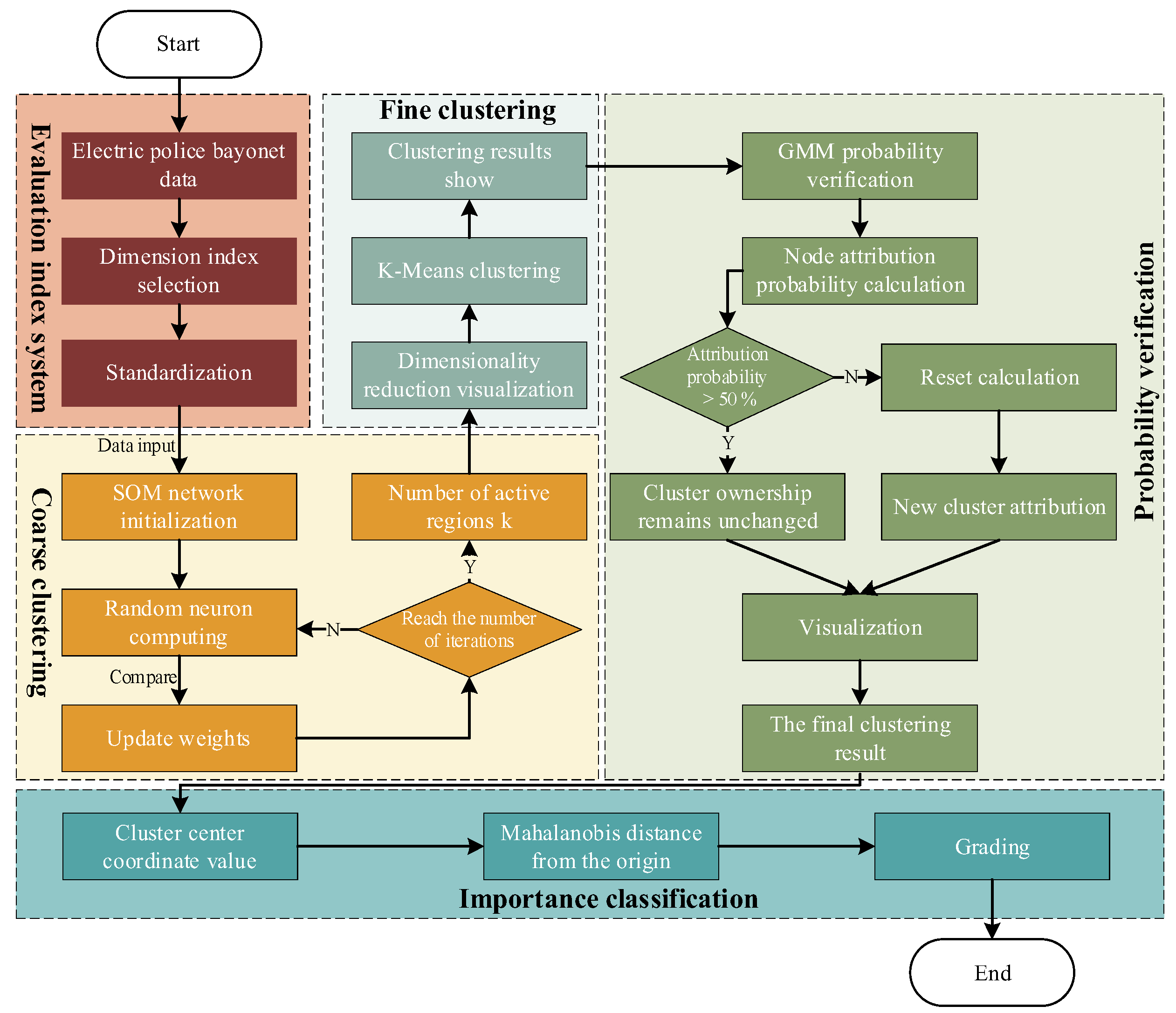
Therefore, this paper introduces a combined SOM-K-GMM clustering method comprising the following five steps: data processing and indicator extraction, SOMs-based coarse clustering, K-Means-based fine clustering, GMM-based probabilistic assignment verification, and importance ranking based on the Mahalanobis distance. The research framework is presented in Figure 1.
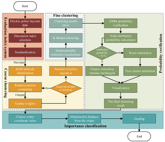
Figure 1.
Flowchart of the intersection importance classification method.
First, the TNS evaluation index system was constructed by comprehensively considering traffic flow, road network structure, and socio-economic factors. The most representative indicators were selected for characterization, and the calculation results were normalized to ensure consistency and comparability.
Based on the constructed TNS indicator system, the SOMs algorithm was applied for the coarse clustering of intersections. Data from six indicators were mapped onto three dimensions, and the number of activated regions k and the corresponding central coordinates were determined, thus eliminating the influence of manually set parameters on the results. This process avoids the cumbersome k-value determination in the K-Means method.
Subsequently, the k-value determined by the SOMs algorithm was used in the K-Means method for fine clustering, thereby optimizing the clustering results through distance-based measures, which enhances clustering accuracy and stability.
Next, the GMM was used for probabilistic verification of the data point cluster membership. The probability of each intersection belonging to the current cluster was validated, and intersections with low probabilities were reassigned to new clusters. This method breaks the limitation of K-Means clustering regions being spherical, enhancing the flexibility of the clustering process and improving overall clustering quality.
Finally, based on the Mahalanobis distance from the cluster center coordinates to the origin, the importance of ranking intersections was determined by time period.
2.2. Construction of TNS Index System
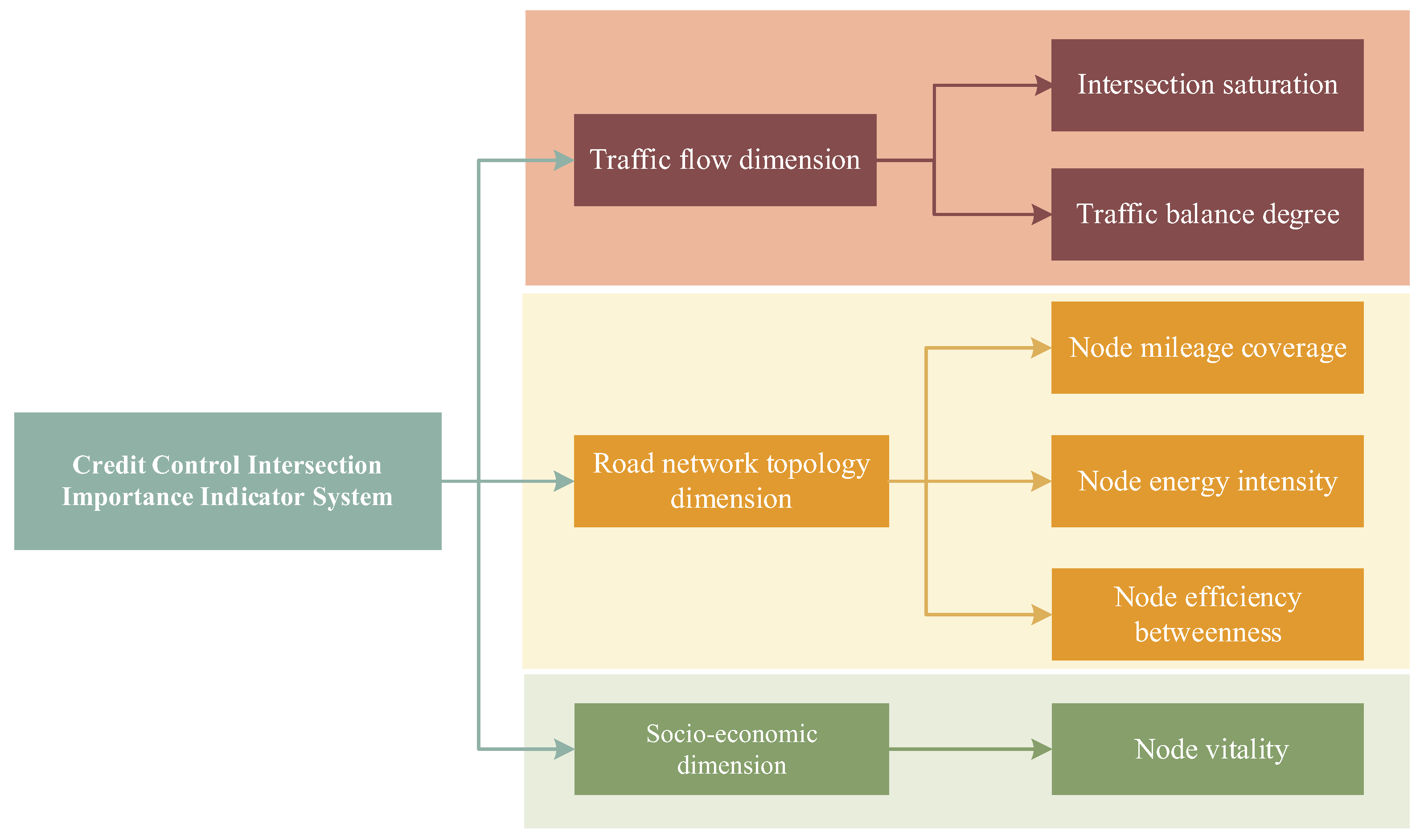
The construction of the evaluation index system plays a critical role in the model and has a significant impact on the results. Drawing upon previous studies [16,18], this paper develops the TNS evaluation index system from three dimensions: one dynamic dimension, the traffic flow dimension, and two static dimensions (the road network topology dimension and the socio-economic dimension). The detailed framework is illustrated in Figure 2. The following analysis was conducted under static conditions.

Figure 2.
Structural diagram of the Importance Grading Index system for signalized intersections.
As shown in Figure 2, the traffic flow dimension primarily focuses on the traffic characteristics of intersections, reflecting the operational efficiency and load conditions of the transportation system. It is measured using two indicators: intersection saturation [24] and traffic balance degree.
The road network topology dimension emphasizes the structure and function of intersections and their connected road segments within the network, capturing the accessibility, connectivity, and efficiency of the road network. It is quantified through three indicators: node mileage coverage [25], node energy intensity [26], and the node efficiency betweenness [27].
The socio-economic dimension reflects the impact and feedback of the transportation system within socio-economic activities, particularly regarding traffic flow. It is evaluated using the node vitality indicator [28], which represents the intensity of social activities around the road network.
2.2.1. Traffic Flow Dimension
- Intersection Saturation
Considering intersection flow alone is insufficient and overly simplistic as it does not account for the design and application characteristics of the intersection. Therefore, intersection saturation was selected as an evaluation indicator [24]. The specific calculation process is as follows:
Step 1: Extract the traffic flow information for each intersection from the traffic flow dataset. Compute the average values and divide them according to hourly time stamps.
Step 2: Calculate the design capacity of each intersection. As all selected intersections are signalized, their organizational capacities differ and must be calculated based on the specific characteristics of each intersection.
Step 3: Compute the intersection saturation and perform dimensionality reduction. Using the original data, construct a 40 × 24 intersection saturation matrix, where 40 represents the number of signalized intersections and 24 corresponds to the hourly time stamps.
Step 4: Perform KMO and Bartlett’s tests, as well as Pearson correlation analysis, on the intersection flow characteristic matrix.
Step 5: Apply principal component analysis (PCA) to reduce the dimensionality of the intersection saturation data matrix.
- 2.
- Traffic balance degree
The road network operates as a typical directed network with complex dynamics. It is insufficient to consider only the traffic flow at an intersection in isolation. Therefore, the flow of each signalized intersection was analyzed, and the reciprocal of the standard deviation of the flow was used to quantify the traffic balance degree. The calculation formula is expressed as follows:
In the formula, represents the traffic balance degree of the intersection labeled i. A larger value indicates a more balanced distribution of flow directions at the intersection; denotes the flow of the n-th direction at intersection i; represents the average flow across all directions at intersection i; and N is the total number of flow directions at intersection i.
2.2.2. Road Network Topology Dimension
Based on the idea of graph theory, the road network is simplified into a topological structure diagram. A general time series network G is then constructed, which includes a point set V and an edge set E (which is composed of finite nodes), and the road network is recorded as .
- Node mileage coverage
Node mileage coverage [25] is calculated as the ratio of the total mileage of road sections connected to a given intersection to the total mileage of the entire road network. From the road network topology dimension, this indicator provides an intuitive representation of the topological characteristics of the road network.
In the above formula, is the actual mileage of the road section from node i to node j, and is the adjacency matrix element of the road network.
- 2.
- Node energy intensity
Node energy intensity [26] is defined as the ratio of the total traffic capacity of the road sections connected to an intersection to the maximum allowable traffic flow provided by all traffic directions at that intersection within the road network. A higher value indicates a more favorable positional significance of the intersection.
In the above formula, is the capacity of the road section from intersection i to intersection j, and is the adjacency matrix element of the highway network.
- 3.
- Node efficiency betweenness
Node efficiency betweenness [27] is calculated as the ratio of the total shortest path efficiency between an intersection and all of the other intersections in the road network to the total path efficiency between all intersections in the network. A higher value indicates greater path efficiency for the intersection, highlighting its critical role in enhancing the overall efficiency of the road network.
In the above formula, is the efficiency betweenness of intersection i; E is the efficiency identification; and is the identification variable that connects intersection j and intersection k, which exists in the m-th shortest path passing through intersection i. If the m-th shortest path exists, then is 1, and vice versa is 0. is the efficiency of the m-th shortest path connecting intersection j and intersection k, and it passes through intersection i. is the number of shortest paths connecting intersection j and intersection k, and it passes through intersection i. ∈{1, 0} is the identification variable for the existence of the m-th shortest path connecting intersection j and intersection k. If the m-th shortest path exists, then is 1, otherwise, it is 0. is the efficiency of the m-th shortest path connecting intersection j and intersection k, and is the number of shortest paths connecting intersection j and intersection k.
2.2.3. Socio-Economic Dimension
In recent research, the concept of point of interest (POI) [28] has been introduced, and the economic vitality of the intersection is described by the node vitality. The node vitality refers to the number of POI adjacent to the node and the average vitality of the intersection within the study area. The specific implementation process is as follows:
Step 1: Download the road network map file and import it into ArcGIS. After loading, extract and record the latitude and longitude of the center point for each intersection, which is labeled according to its identifier.
Step 2: Using the mileage coverage index, determine the shortest search radius for the POI points. The final search radius is set to 250 m.
Step 3: Use Python (version 3.9) to retrieve the POI data within the specified radius for each intersection. Retrieved POI categories include hospitals, educational institutions, shopping malls, companies, etc.
Step 4: Traverse all intersections, calculate the results, and classify them using Excel.
Step 5: Apply the formula to calculate the node vitality for each intersection. The specific calculation formula is as follows:
In the above formula, is the vitality index of the i-th intersection, is the number of important vitality points of the i-th intersection, and N is the total number of intersections in the study area.
2.3. Construction of the Clustering Algorithm Model
2.3.1. SOMs Neural Network Coarse Clustering
The SOMs algorithm is widely used in unsupervised learning and data dimensionality reduction. Compared to other methods, such as PCA, MDS, and t-SNE, it offers superior visualization capabilities while preserving the topological structure of the data. Additionally, it exhibits greater computational power when applied to larger datasets [29]. The construction steps of the SOMs algorithm are as follows:
Step 1: A composition of neurons is created, with each neuron representing a point in the data space. The m-th neuron is selected, and its weight vector is initialized, with the same dimensionality as the data dimension .
Step 2: Random sample input and normalization processing, where a cluster is randomly selected from the dataset as the network input, is conducted.
In the above formula, n represents the dimension of the input vector; m represents the number of neurons in the competitive layer; and are the Euclidean norm of the input vector and the weight vector, respectively.
Step 3: Adapt the best neuron and its topological neighborhood with the following:
The topological neighborhood is determined based on the calculation of the neighborhood function .
In the above formula, refers to the distance between the winning neuron M and the other neurons, and denotes the size of the neighborhood.
Step 4: The weights of neighboring neurons are updated, after finding the most suitable neuron, by adjusting the weights of the winning neuron and its neighboring neurons. The adjusted weights are then renormalized, and the learning rate λ(t) and the neighborhood size σ(t) are updated.
In the above formula, represents the weight vector of neuron m at time t. denotes the learning rate at time t, which controls the step size for weight updates. is the neighborhood function value between neuron m and the winning neuron M at time t, indicating the degree of influence that M exerts on neuron m. represents the input vector. denotes the updated weight vector of neuron m at time t + 1.
The physical significance of weight updating lies in adjusting the neuron’s weight to better approximate the input vector . The winning neuron and its neighboring neurons update their weights based on the input vector, with the magnitude of adjustment determined by both the learning rate and the neighborhood function. This mechanism facilitates the formation of an orderly topological structure within the SOMs, ensuring that similar input vectors are mapped to adjacent neurons in the network.
Step 5: Repeat Steps 2 to 4 until convergence. Visualize the SOMs results and output the optimal number of neurons along with their coordinates.
2.3.2. K-Means Fine Clustering
The K-Means method is a classical clustering algorithm [30] that mainly finds the center of the cluster through iterative optimization, the calculation of which is cumbersome. However, in this study, the number of activation regions, namely the k value, was obtained through the coarse clustering of the SOMs algorithm, which can avoid the complex process of verifying the k value one by one. Due to this, the K-Means method can then directly apply the k value to the fine clustering analysis of the intersection. The specific steps of this are as follows:
Step 1: Use the SOMs algorithm to determine the number of active regions, namely the k value.
Step 2: Determine the clustering according to the k value and the center coordinates of the activation area by the SOMs algorithm.
Step 3: Calculate the Euclidean distance from each data point to each cluster center and cluster attribution.
In the above formula, represents the Euclidean distance from the i-th data point to the j-th cluster center; , , and are the coordinate components of the i-th data point in the TNS index system; and , , and are the coordinate components of the j-th cluster center.
Step 4: Complete the K-Means clustering and visual display to obtain the clustering effect diagram.
2.3.3. GMM Probability Verification
The GMM is a probabilistic model used to represent complex data distributions comprising multiple Gaussian components. Its fundamental structure includes mixture components, weights, means, and covariances, which are expressed as a weighted sum of multiple Gaussian distributions [31]. Since the clusters obtained through the K-Means method are spherical, centered around the cluster centroids, this can result in assignment biases for certain intersections. By applying GMM, each point undergoes a reevaluation of its cluster membership probability, allowing adjustments to the cluster assignment of specific intersections. This enhances the rationality and accuracy of the clustering results. The construction steps are as follows:
- Formula composition
① The mixed-density function is as follows:
where x is the data sample; k is the number of mixed components; is the weight of the k-th Gaussian distribution; and represents the probability density function of the k-th Gaussian distribution with mean and covariance .
② The specific expression of the probability density function is as follows:
In the above formula, D is the dimension of data, is the determinant of the covariance matrix, is the inverse matrix of the covariance matrix, and is the transpose of vector .
- 2.
- Parameter estimation
In the Gaussian mixture model, the expectation maximization (EM) algorithm is usually used to estimate the parameters. This includes the following two steps:
① Expectation step (E): According to the specified initial value, or the mean, and the covariance and mixed weight obtained in the iterative process, the posterior probability of each data point belonging to each Gaussian component is calculated.
② Maximization step (M): The model parameters are updated according to the posterior probability calculated in Step E, and the new mean, covariance, and mixed weights are obtained using the maximum likelihood method.
where represents the mean of the k-th Gaussian distribution in the i-th iteration; denotes the posterior probability of the j-th data point belonging to the k-th Gaussian distribution; is the j-th data point; represents the covariance matrix of the k-th Gaussian distribution in the i-th iteration; represents the mixing weight of the k-th Gaussian distribution in the i-th iteration; and N is the total number of data points.
③ Calculate the EM value repeatedly until the convergence condition is satisfied:
Finally, the parameter values of the Gaussian mixture model are obtained. The Gaussian mixture model can effectively capture the complex patterns and structures in the data. Using the EM algorithm, the parameters of the model can be optimized according to the data so as to achieve good modeling of the probability verification of the clustering results.
2.4. Intersection Classification Based on Mahalanobis Clustering
Based on the clustering results, the hierarchical classification of intersection importance was conducted. Simply relying on clustering outcomes is insufficient to indicate the importance levels of intersections. During the SOMs-based preliminary clustering, the number of activation regions k was determined, thus dividing the intersections into k levels of importance. Considering the correlations between certain features, the Mahalanobis distance was utilized to rank the clusters. The importance level of intersections is represented by the D between the cluster centroids and the coordinate origin. A larger D value indicates a higher importance level for the intersection. The detailed calculation steps are as follows:
Step 1. (Dataset Construction): Construct the dataset X with dimensions m × n, where m represents the number of intersections and n represents the number of features.
Step 2. (Data Standardization:): Ensure that data standardization has been completed during the calculation of each indicator.
Step 3. (Calculation of Mean Vectors): Compute the mean vector for the data points in each cluster. This vector represents the average values of all the features within the i-th cluster.
In the above formula, represents the mean value of the j-th feature, represents the value of the i-th sample for the j-th feature, and m denotes the total number of samples.
Step 4. (Calculation of the Covariance Matrix S for Each Cluster): Each element in the covariance matrix is defined by the following formula:
The covariance matrix S is obtained as follows:
In the above formula, represents the covariance between the i-th and j-th features; and represent the values of the i-th and j-th features, respectively; denotes the value of the i-th feature in the k-th sample; and are the mean values of features and , respectively; and represents the covariance between features and .
Step 5. (Calculation of the D): Using the coordinate origin as the reference vector (the zero vector), the Mahalanobis distance is calculated using the following formula:
In the above formula, x is the mean vector of the cluster; 0 is the zero vector, representing the origin; and is the inverse of the covariance matrix S.
3. Example Verification and Discussion Analysis
3.1. Database Construction
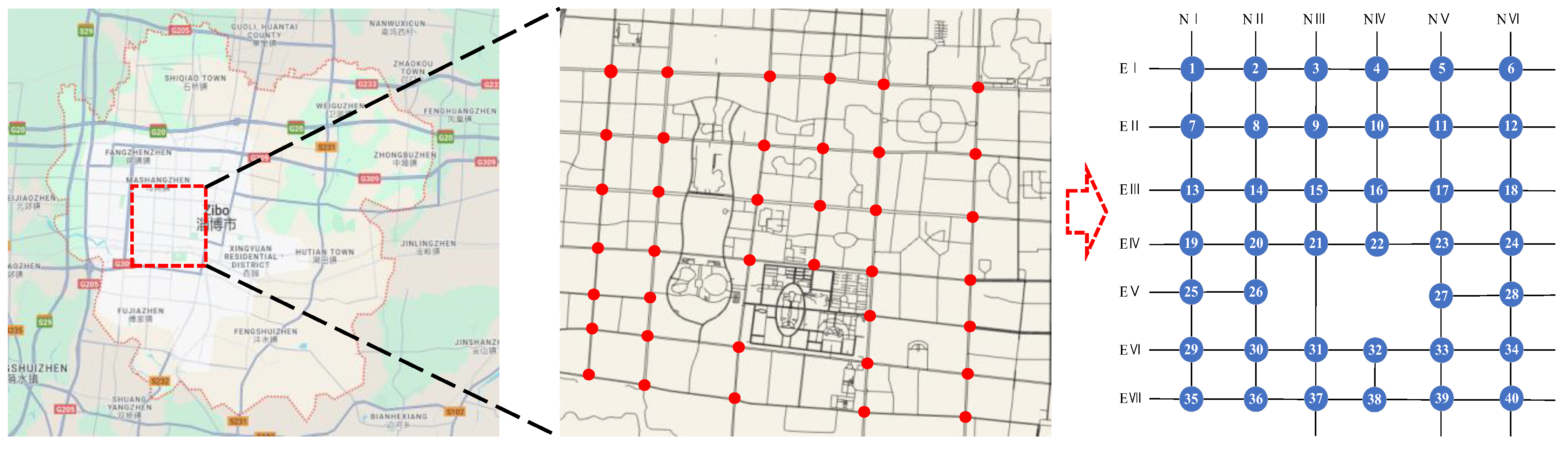
The traffic flow data used in this study were obtained from electronic police checkpoint devices located at 40 signal-controlled intersections within the road network of Zibo City. This study area provides abundant vehicle flow data, meeting the requirements of the research. The map data were sourced from the OpenStreetMap (OSM) platform, and the map scaling and processing workflow is illustrated in Figure 3.
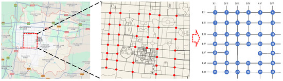
Figure 3.
A diagram of the study of the scale extension of regional signalized intersections.
The raw dataset includes desensitized license plate information (with the license plate registration location and the last three digits of the plate number concealed), the vehicle’s travel direction, passing time, lane number, and other details, totaling 40 million records. The specific data types are shown in Table 1.

Table 1.
Data examples.
3.2. Indicator Calculation
3.2.1. Calculation Process of Intersection Saturation Degree
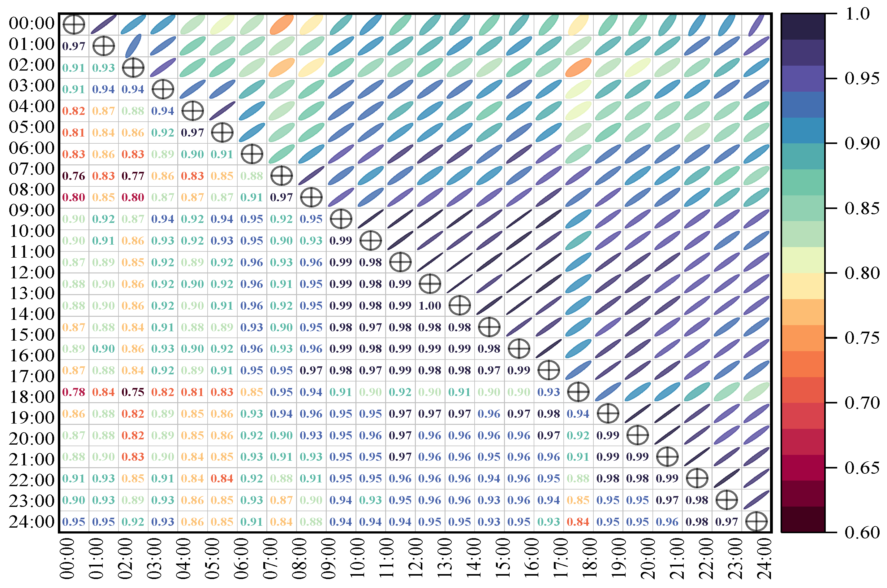
Dimensionality Reduction of Intersection Saturation Degree Based on the Steps in Section 2. First, the KMO test and Bartlett’s test were conducted on the traffic flow matrix of a given intersection. The specific test results are shown in Table 2. Additionally, a heat map of Pearson correlation coefficients at different time periods at the intersection was generated, as presented in Figure 4.
Table 2.
The KMO and Bartlett tests.
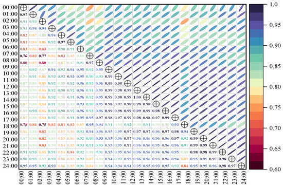
Figure 4.
Correlation heat map of the intersection saturation.
After completing the tests, PCA was applied to the intersection saturation degree data matrix for dimensionality reduction. The top five principal components in terms of cumulative contribution are presented in Table 3.
Table 3.
Total variance explanation.
The first principal component exhibits a contribution rate of 92.163%, exceeding 85%, which indicates its strong representation of the overall characteristics. Therefore, the first principal component is selected for the subsequent indicator calculation.
3.2.2. Spatial Characteristics of Intersection Index
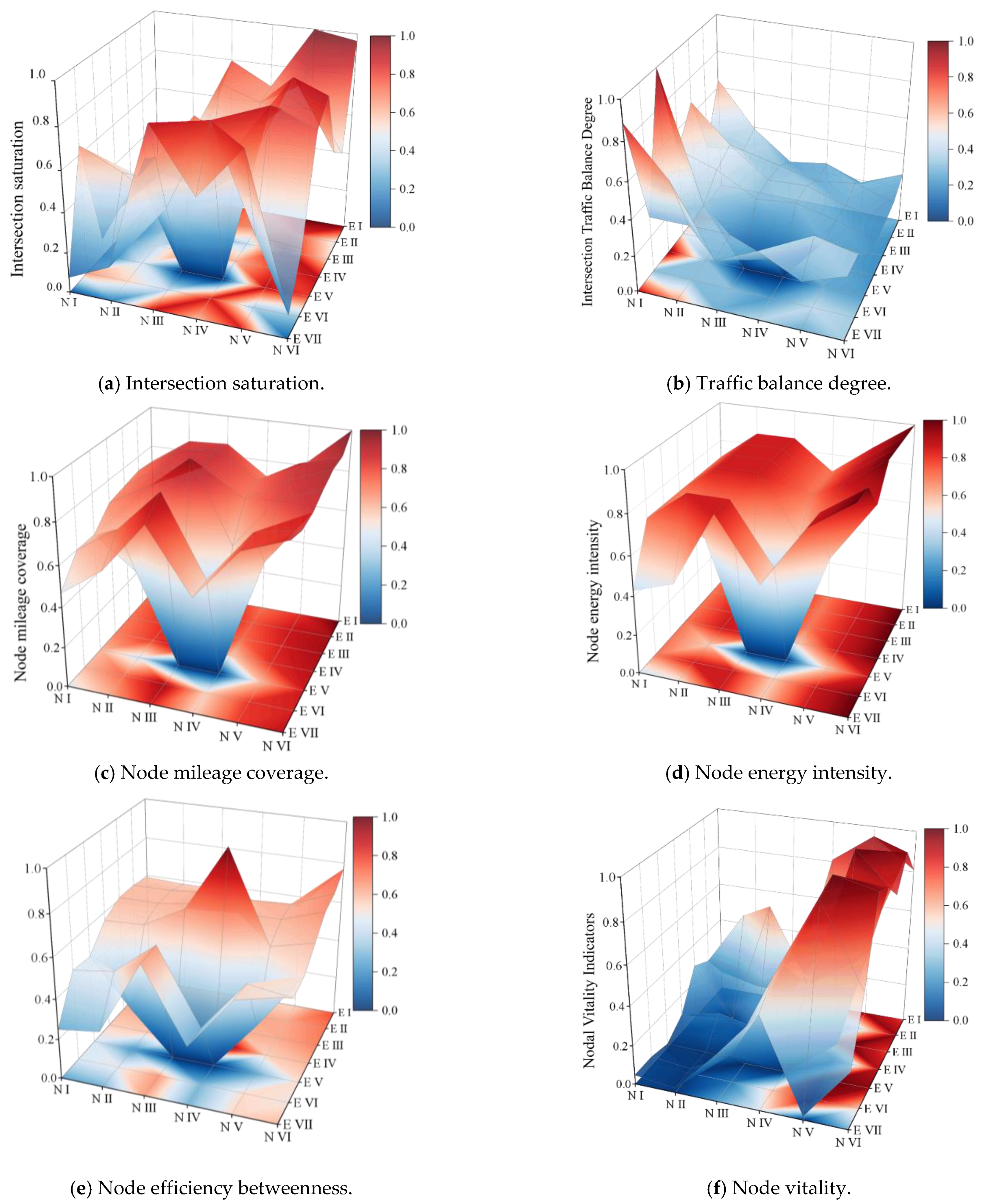
The six selected indicators were computed and standardized based on the study data, resulting in a three-dimensional mapping of the road network, as illustrated in Figure 5. Spatial representation for each indicator was conducted within the three dimensions. A boxplot depicting the overall distribution of intersection importance based on the six indicators was also generated, as shown in Figure 6.

Figure 5.
Index-standardized spatial feature map.
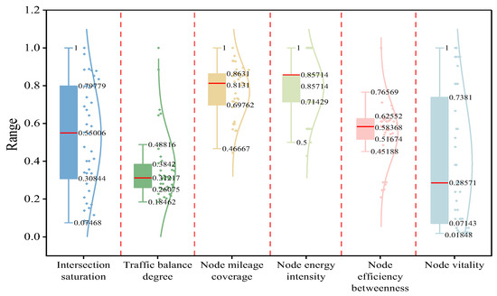
Figure 6.
Distribution box plot of each index calculation.
- Traffic flow dimension
- ➀
- As shown in Figure 5a and Figure 6, the scores for the intersection saturation indicator under static conditions exhibited distinct differences while maintaining a relatively uniform distribution. Approximately 50% of intersections fell within the range of 0.31–0.79, demonstrating clustering tendencies and continuity across the road network. This indicates that 90% of intersections within the study area operated under smooth or slightly congested traffic conditions, while a few intersections experienced congestion. Notably, these congestion-prone nodes significantly impacted the normal operation of the traffic network and should be prioritized for further analysis and management.
- ➁
- According to Figure 5b and Figure 6, the maximum value of the normalized flow balance index was 0.49, the middle index was 0.31, and 50% of the intersections were distributed in the range of 0.18–0.38 (except for individual intersections). From the point of view of node saturation, the equilibrium degree of nodes with higher saturation was relatively low, which indicates that when a node bears higher traffic pressure, the flow distribution in all directions is unbalanced. This proves that it is necessary to add the flow equilibrium degree when constructing the traffic flow dimension.
- Road network topology dimension
- ➀
- As shown in Figure 5c,d and Figure 6, the degree and energy intensity of each node in the study area were similar, with a maximum value of 1 and minimum values of 0.70 and 0.71, which proves that the intersection was evenly distributed in space. This thus meant that the traffic conditions in the study area were representative and universal. It also reflected the fact that the connectivity between the nodes of the traffic network was good, which means that the vehicles could flow smoothly between different intersections. However, the data distribution of the two was different. The median value of the degree in the node was 0.81, and the distribution was scattered, while the median value of the node energy strength was as high as 0.86. In addition, the data distribution showed obvious aggregation, indicating that there were key nodes in the network. They had high connection ability and played an important role in the overall performance and stability of the road network. The distribution concentration of node energy intensity may imply that some of the nodes in the network played a core role in information dissemination and resource allocation. At the same time, the degree of dispersion in the nodes may indicate that the connections in the network were more uniform and that there was no obvious centralization trend.
- ➁
- As shown in Figure 5e and Figure 6, 80% of the data distribution was 0.25–0.63, which was in the medium situation, except for the high value of the node performance betweenness at individual points. This showed that most of the nodes were of moderate importance in the traffic network, which was neither an absolute traffic bottleneck nor a completely irrelevant node. This medium level of node effectiveness betweenness may mean that the traffic flow distribution in the traffic network was relatively balanced and that there was no excessive concentration or dispersion.
- Socio-economic dimension
As shown in Figure 5f and Figure 6, in terms of the node activity index, the maximum value was 1 and the minimum value was 0.02, and the data were concentrated in the range of 0.07 to 0.74, indicating that there was polarization in the distribution. The node activity index showed great volatility and aggregation. This aggregation may mean that these nodes have some similarity in function, location, or influencing factors.
Overall, the calculation results of these six indicators revealed that, under static conditions, the intersections within the study area exhibited variations due to differences in traffic organization, lane division, road structure design, and surrounding economic conditions. These characteristics are crucial for achieving intersection classification and can be effectively utilized in the proposed SOM-K-GMM hybrid method to classify the importance of signal-controlled intersections.
3.3. Importance Classification of Intersections
3.3.1. Comparison Under the Same Conditions
This study applies, using a static example, the proposed method to classify the importance of intersections in an urban road network. First, this method applies the SOMs algorithm to perform coarse clustering, thereby determining the optimal number of neurons, thus avoiding the complex determination of k in the K-Means method. Subsequently, the K-Means method is applied for fine clustering based on the results. Finally, the GMM is utilized to compute the assignment probabilities of the data points within the clusters, further refining the clustering process and overcoming the limitations of circular clustering areas inherent in the K-Means algorithm. The detailed results are as follows:
- SOMs neural network rough clustering
The SOMs neural network was used to learn the index dataset, and the dimension reduction and mapping of the six indicators were carried out to obtain the number of active regions k and the coordinate value of the cluster center. The black dots represent the corresponding data points of each intersection after dimensionality reduction. The visualization results are shown in Figure 7, and the calculation results are shown in Table 4.
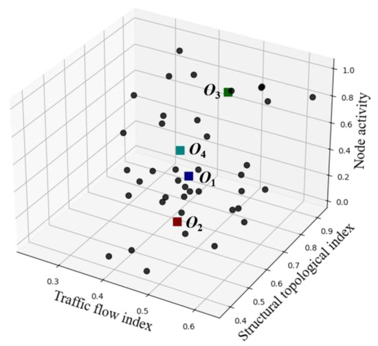
Figure 7.
Visualization of the SOMs neural network coarse clustering.
Table 4.
Cluster center and activation area.
- 2.
- K-Means method for fine clustering
Using the k-value and corresponding coordinate centers determined by the SOM-based coarse clustering, the k-means algorithm is then applied. After clustering, each cluster is color-coded, and the data points within the same cluster are enclosed with an ellipse (Figure 8).
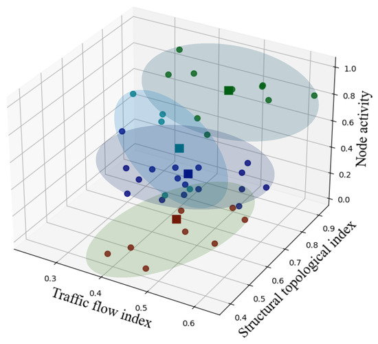
Figure 8.
Visualization of the K-Means clustering results.
- 3.
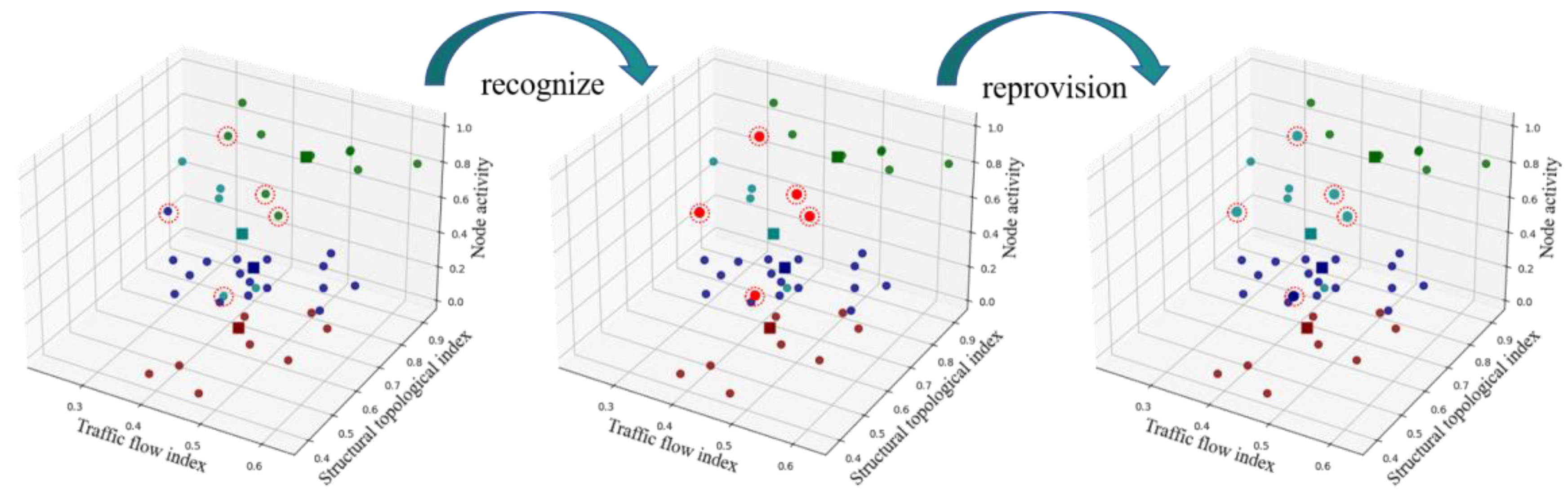
- GMM Gaussian mixture model validation
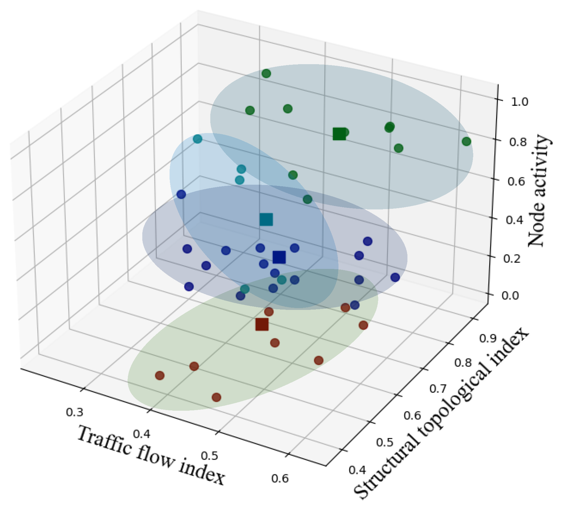
The GMM Gaussian mixture model was used to verify the probability of cluster attribution of each node, and the nodes with attribution values greater than 50% were corrected. To enhance clarity, data points with low membership values are highlighted with a red circle and reassigned to the appropriate cluster. The final SOM-K-GMM clustering results are shown in Figure 9.
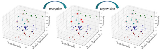
Figure 9.
The final results of the SOM-K-GMM combined clustering.
- 4.
- Importance classification results of the intersections
In the SOMs coarse clustering, the number of activation areas was determined to be four; that is, the intersection was divided into four levels according to importance. In this paper, the four levels are defined as follows: key intersections, important intersections, secondary intersections, and ordinary intersections. The calculation results, in accordance with Formula (20) and the cluster center coordinate points, are shown in Table 5.
Table 5.
The importance classification of intersections.
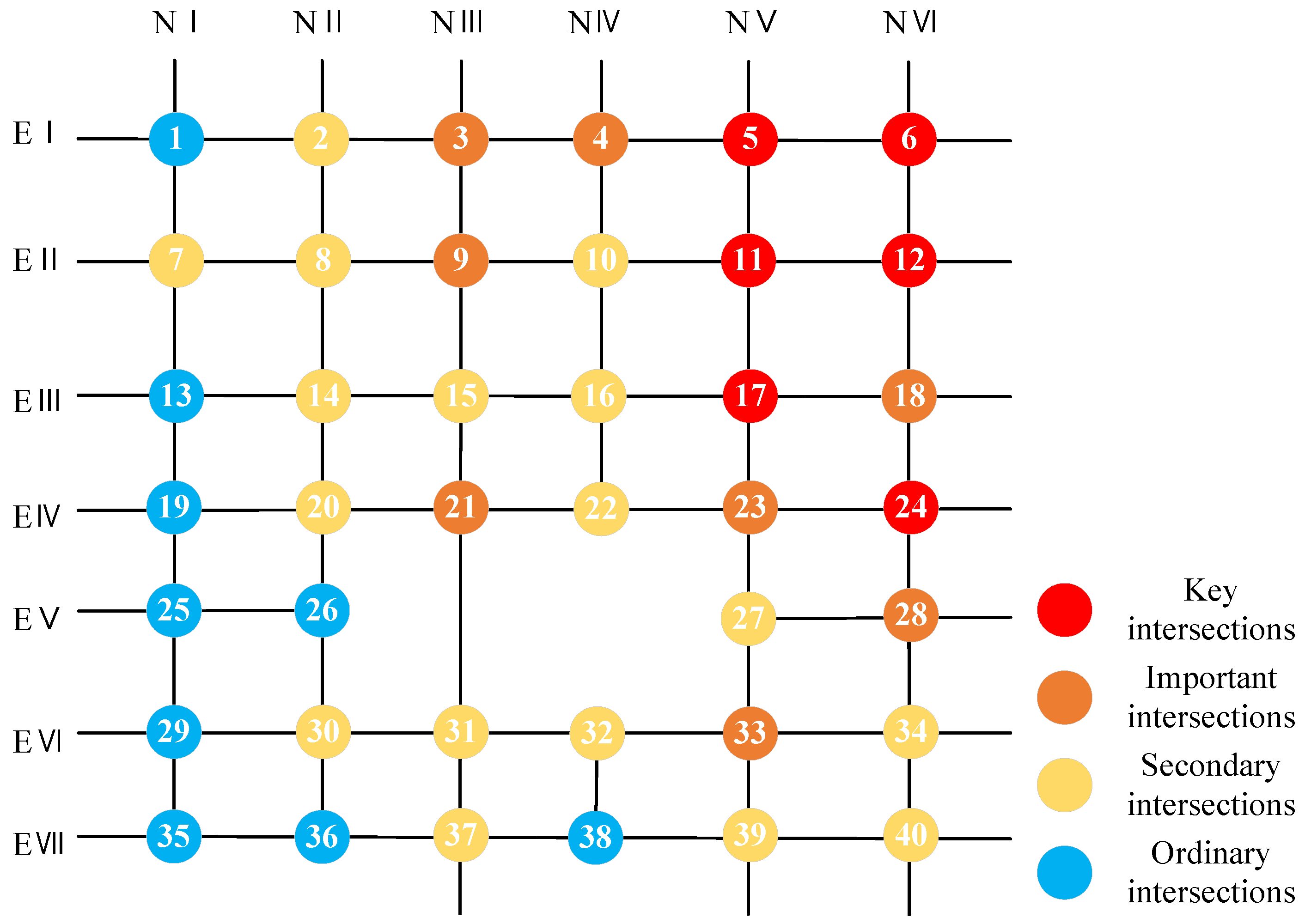
In accordance with the calculation results of Table 5, the importance level distribution map of intersections was finally drawn in the road network topology map, which is shown in Figure 10. Finally, the signalized intersections were divided into four levels, including 6 key intersections, 8 important intersections, 17 secondary intersections, and 9 ordinary intersections.
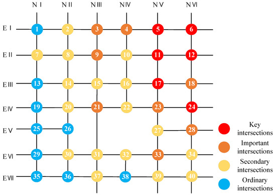
Figure 10.
Spatial distribution of the intersection importance in urban traffic signal-controlled intersections.
- 5.
- The results of clustering analysis
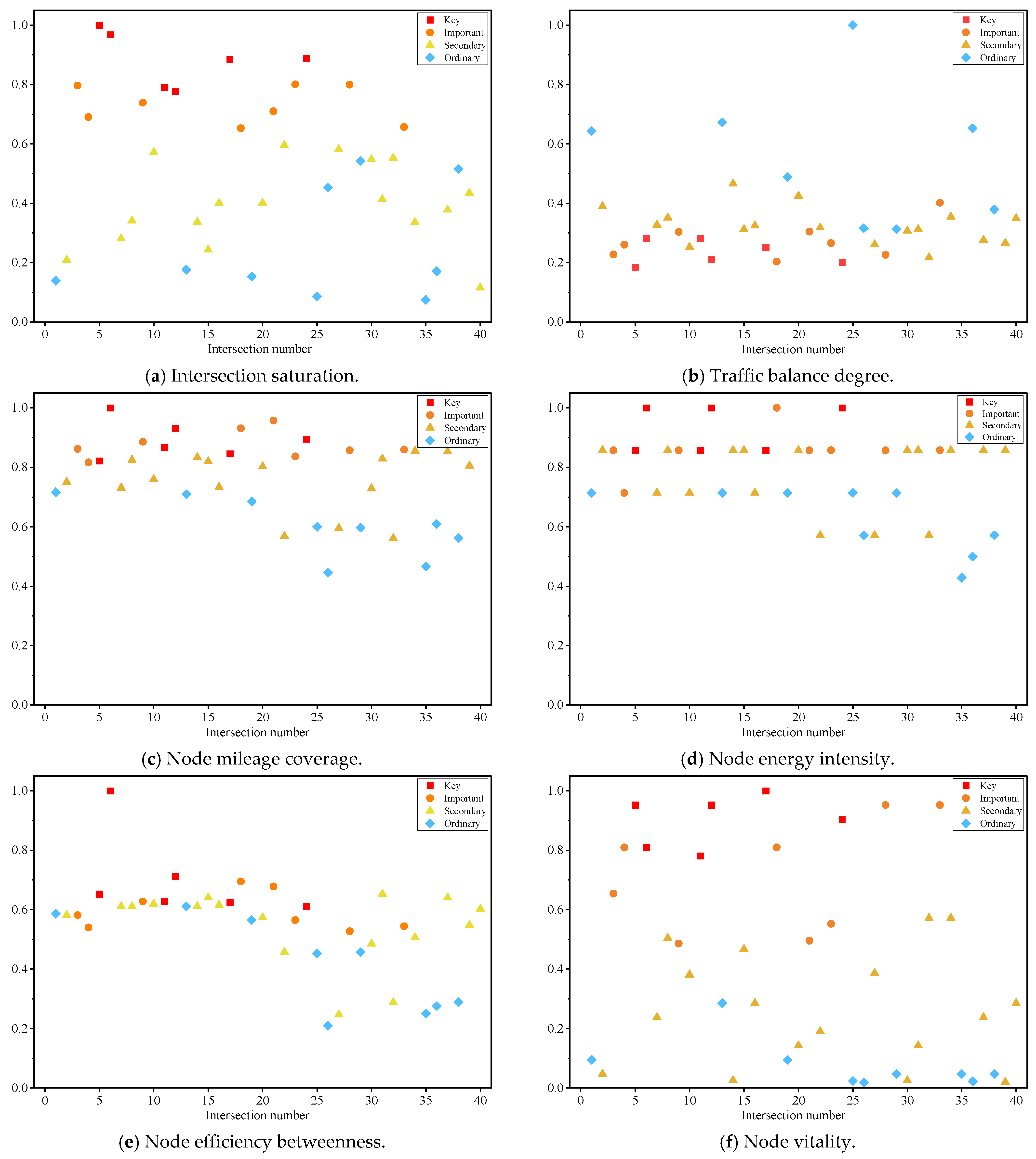
By analyzing the clustering outcomes together with the actual conditions of the intersection importance indicators, the normalized indicator values for each intersection are presented in Figure 11.
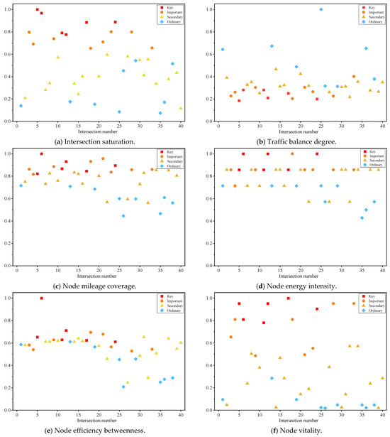
Figure 11.
Distribution of Normalized Indicator Values.
- ➀
- As shown in Figure 11a,b, within the traffic flow dimension, the results for the intersection saturation indicator reveal that critical intersections have the highest values, followed by important intersections. This finding indicates that higher intersection saturation corresponds to greater intersection importance. Meanwhile, regarding the traffic balance degree, larger values represent more evenly distributed flows across different directions. However, both critical and important intersections exhibit relatively low flow balance, implying that unbalanced traffic may lead to congestion and thus underscore the significance of these intersections. Overall, the clustering outcomes for these two indicators align well with actual conditions.
- ➁
- As illustrated in Figure 11b–d, within the road network topology dimension, the three indicators—node mileage coverage, node energy intensity, and node efficiency betweenness—exhibit a similar pattern. Critical intersections and important intersections display relatively high values, whereas secondary and normal intersections present lower values. These findings indicate that larger values in these metrics correspond to greater capacity in the road network topology dimension, thus reflecting a higher level of intersection importance.
- ➂
- As depicted in Figure 11f, within the socio-economic dimension, the normalized results of the node vitality indicator reveal that intersections situated in areas with higher economic vitality exhibit higher vitality values. Consequently, such intersections draw greater traffic flows, which in turn elevates their importance level. These findings underscore that an intersection’s significance is closely tied to the surrounding socio-economic context.
- ➃
- As illustrated in Figure 11, there is no clear boundary among intersections of different importance levels in certain indicators, particularly when comparing secondary intersections with normal intersections. Therefore, relying solely on a single indicator or subjective evaluation methods for intersection importance classification is generally insufficient. A comprehensive consideration of multiple intersection attributes is necessary to achieve an objective importance ranking.
In summary, a comprehensive analysis of the clustering results combined with real-world road network conditions confirms that the classification outcomes align well with actual intersections, thereby validating the scientific rigor and rationality of the cluster-based intersection importance classification method. This approach has demonstrated practical significance and can serve as a valuable reference for urban road traffic management decisions.
3.3.2. Comparison Under Different Conditions
This study conducted importance classification of the intersections for four conditions: off-peak hours, morning peak hours, evening peak hours (each represented by a one-hour period), and static conditions. The detailed results are presented in Table 6.
Table 6.
The importance classification results across different time periods.
The results shown in Table 6 reveal the variation trends in the number of nodes across different importance levels during various time periods. They provide valuable insights into how the importance hierarchy of the traffic network changed over time, offering significant implications for the optimal allocation of urban traffic resources and dynamic traffic management. The specific characteristics are as follows:
- Temporal Variation Characteristics of the Traffic Node Distribution
Static Condition: Under static conditions, traffic volumes are low, and traffic demand is evenly distributed. Only a small number of nodes exhibit significant importance. Off-Peak Period: During off-peak hours, the traffic flow remains relatively uniform, with 70% of nodes classified as “ordinary” level, and this indicates that no special considerations are required for control strategies or resource allocation during this period. Morning Peak Period: In the morning peak, multiple intersections simultaneously experience significant pressure, necessitating targeted management and resource allocation to ensure smooth traffic flow across the network. Evening Peak Period: During the evening peak, the node demands either remain consistent with or slightly exceed those of the morning peak, and this reflects a more concentrated travel demand during evening hours, thus requiring careful consideration of resource allocation and traffic control measures.
- 2.
- Dynamic Evolution of Node Importance Over Time
The number of “secondary” nodes was highest under static conditions but decreased significantly during the peak periods. This suggests that the nodes originally deemed less important assumed a greater share of traffic flow during peak hours. The number of “ordinary” nodes peaked during off-peak hours but declined during peak periods. This indicates that more nodes were classified into higher importance levels during peak hours, necessitating adjustments in the management strategies and resource allocation to accommodate the increased traffic demand.
In summary, the node importance exhibited dynamic variations across different time periods, highlighting the differing traffic management demands during these intervals. Such differences necessitate deliberate intervention to enable rational traffic control, reduce congestion, enhance the overall efficiency of the network, and minimize resource wastage.
3.3.3. Comparison of the Same Intersection Across Different Conditions
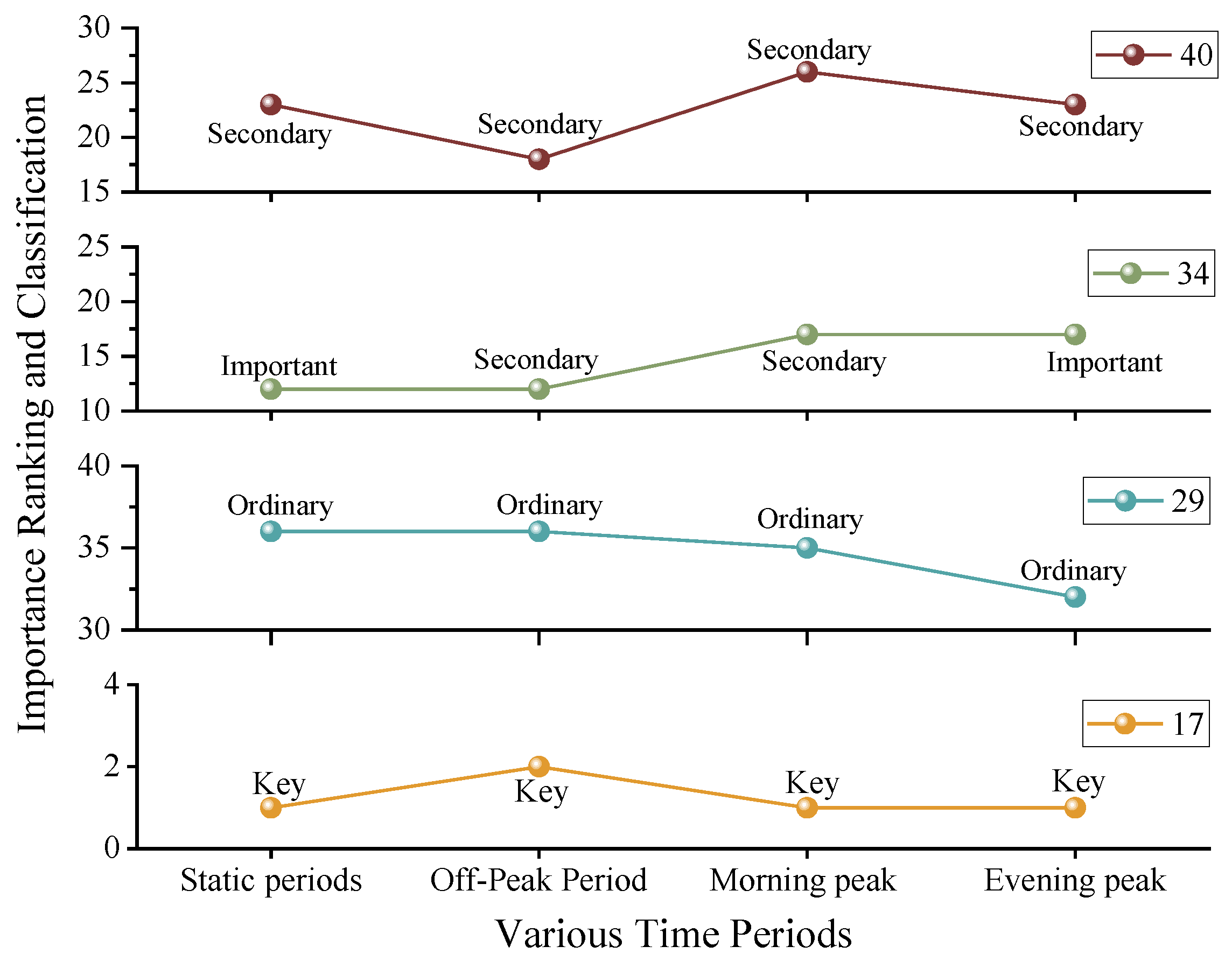
In this section, four intersections were selected for analysis, comparing their importance classification and ranking across different time periods. The intra-cluster ranking was determined using the Mahalanobis distance. The specific importance rankings and classification results are presented in Figure 12.
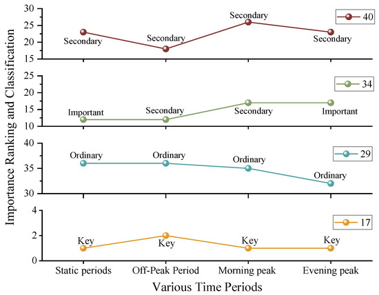
Figure 12.
A line chart of the intersection importance rankings.
As shown in Figure 12, the importance rankings of the four intersections exhibit a certain degree of fluctuation, with some intersections experiencing changes in classification. The specific observations are as follows:
- Intersections No. 17 and No. 40 maintained consistent classification across all time periods, including the static state, morning peak, off-peak, and evening peak periods. This indicates that these intersections remain stable within the road network. Intersection No. 17 has consistently been classified as a key intersection, demonstrating its crucial role in the road network. Traffic management authorities should prioritize its monitoring and continuously optimize its operation to ensure smooth traffic flow. Intersection No. 40 has consistently been classified as a secondary intersection, indicating relatively low importance. Traffic management departments only need to allocate minimal resources to ensure its normal operation. This allows more resources and attention to be focused on key intersections, thereby enhancing overall road network efficiency and preventing unnecessary resource wastage.
- Intersections No. 29 and No. 34 showed classification fluctuations throughout the day. In the static classification, Intersection No. 29 was categorized as an ordinary intersection, while Intersection No. 34 was classified as an important intersection. However, during different time periods throughout the day, such as the morning and evening peak hours, their classifications changed. These fluctuations are primarily caused by variations in traffic flow within the road network. The changes in importance classification during peak hours suggest that these intersections require increased attention. Traffic management authorities should allocate resources dynamically based on these variations to ensure smooth and safe traffic flow within the network.
3.4. Clustering Algorithm Effect Evaluation
The contour coefficient, Davies–Bouldin index, and Calinski–Harabasz index were used to evaluate the proposed method [32,33]. The contour coefficient represents the tightness and separation of the cluster. Its value is between [−1, 1], and the closer it is to 1, the better the clustering effect of the model is. The Davies–Bouldin index represents the ratio of the similarity within the class to the discrimination between the classes, and its value is greater than 0. The smaller the value is, the better the clustering effect of the model is. The Calinski–Harabasz index represents the ratio of inter-class dispersion to intra-class dispersion, and the larger the value, the better the clustering effect of the model. The SOM-K-GMM combined clustering method and the other methods used in this paper were tested for contour coefficients. The silhouette coefficient is calculated as follows:
where represents the average distance between data point i and all other points within the same cluster, while denotes the average distance between data point i and all points in the nearest neighboring cluster.
By computing the silhouette coefficient for all data points and averaging the results, the final silhouette coefficient for the clustering method in this study is obtained. The results are shown in Table 7.
Table 7.
Comparison of the SOM-K-GMM combination method with other methods.
According to Table 7, the SOM-K-GMM method achieved a silhouette coefficient of 0.737, a Davies–Bouldin index of 1.003, and a Calinski–Harabasz index of 57.688, indicating an overall improvement in clustering performance. Within this area of research, previous studies have explored methods for determining the k value in K-Means, with some proposing the integration of the SOMs algorithm and the analytic hierarchy process for this purpose. In subsequent clustering processes, the SOMs algorithm has been incorporated to enhance clustering models, yielding a silhouette coefficient of 0.661. Additionally, a clustering framework combining K-Medoids, random forests, and fuzzy C-means has been introduced to address the issue of clustering shape, achieving a silhouette coefficient of 0.705.
The proposed method demonstrated a 78.1% increase in the silhouette coefficient compared to the standalone SOMs algorithm, corresponding to a 65.2% improvement over the K-Means method, an 11.5% increase over the SOM-K-Means method, and a 4.6% enhancement compared to the modified fuzzy C-means method. Compared to traditional clustering approaches, the SOM-K-GMM method exhibited higher efficiency and accuracy in processing large-scale traffic flow data. The superior silhouette coefficient further confirmed the method’s ability to distinguish between different data groups while maintaining internal cohesion effectively. These findings reinforce the robustness and effectiveness of the proposed approach.
4. Conclusions
This study proposed a SOM-K-GMM clustering method to classify the importance of signalized intersections. The key contributions and findings are as follows:
- The TNS evaluation index system assesses signalized intersections from three key perspectives. Analysis of six normalized indicators highlights the significant influence of traffic organization, lane division, road structure, and surrounding economic conditions on intersection classification, providing a basis for the importance classification of signalized intersections.
- Compared with the traditional K-Means method and other optimization methods, the method proposed in this study applied the SOMs method for rough clustering to determine the k value, thus avoiding the iterative process of exploring the k value; in addition, the GMM method was used to calculate the cluster attribution rate of each data point, which overcomes the limitation of the K-Means spherical clustering region.
- The proposed method achieved a silhouette coefficient of 0.737, representing a 78.1% improvement over the standalone SOMs method, a 65.2% improvement over the K-Means method, an 11.5% improvement over the SOM-K-Means method, and a 4.6% improvement over the modified fuzzy C-means method. This demonstrates its superior robustness and accuracy.
- This study establishes an importance-based classification scheme for signalized urban intersections, offering substantial practical implications for urban traffic management and sustainable development. The specific details are as follows:
- ➀
- Provide data-driven support for transportation authorities to allocate resources more efficiently, thereby reducing traffic resource waste.
- ➁
- Offer a foundation and direction for upgrading and renovating urban intersection infrastructure.
- ➂
- Adapt to temporal fluctuations, enabling more refined and dynamic decision-making in urban traffic management.
This study has developed an importance-based classification system for urban intersections from a scientifically rigorous and methodologically sound perspective. Although the findings are significant, certain limitations remain and should be addressed in future research:
- Insufficient sample coverage: The sample range of this study was relatively limited as it was mainly concentrated at intersections in specific areas. Future research can be extended to more urban and regional intersections to enhance the universality and practicality of the method.
- Computational complexity: Although the SOM-K-GMM method improves the clustering efficiency to a certain extent, it may still face the problem of high computational complexity when dealing with particularly large-scale datasets. Future research can further optimize the algorithm, improve its computational efficiency, and reduce resource consumption.
Future research could look to explore how to adapt the method to different urban characteristics by incorporating changes in traffic flow, road network topology, and socio-economic dimensions. In the process of determining the k value, future research will consider a comparative analysis with co-optimization clustering methods and conduct a more detailed validation of the model’s performance from both internal and external perspectives.
Author Contributions
Conceptualization, Z.Y., Y.C. and F.S.; methodology, Z.Y.; software, D.G. and Y.C.; validation, Z.Y., Y.C. and F.S.; formal analysis, B.Z.; investigation, F.J. and B.Z.; resources, D.G., F.J. and F.S.; data curation, Z.Y. and B.Z.; writing—original draft preparation, Z.Y.; writing—review and editing, F.S.; visualization, Y.C.; supervision, F.S.; project administration, D.G. and F.J.; funding acquisition, D.G., B.Z. and F.S. All authors have read and agreed to the published version of the manuscript.
Funding
This work was supported by the National Natural Science Foundation of China (52172314); the Special Funding Project of Taishan Scholar Engineering; the Natural Science Foundation of Shandong Province, China (ZR2024MG021); the Shandong Provincial Programme of Introducing and Cultivating Talents of Discipline to Universities: Research and Innovation Team of Intelligent Connected Vehicle Technology (2021SLG08); and the State Key Lab of Intelligent Transportation System (2024-B009).
Institutional Review Board Statement
Not applicable.
Informed Consent Statement
Not applicable.
Data Availability Statement
Some of the data in this study are contained within the article, and additional data are available upon request from the corresponding authors.
Acknowledgments
We are thankful to the editor and to the anonymous reviewers for their pertinent questions and suggestions to improve this paper.
Conflicts of Interest
The authors declare no conflicts of interest.
References
- Barthelemy, M. The role of parsimonious models in addressing mobility challenges. NPJ Sustain. Mobil. Transp. 2024, 1, 11. [Google Scholar] [CrossRef]
- Wu, P.; Chen, T.; Wong, Y.; Meng, X.; Wang, X.; Liu, W. Exploring key spatio-temporal features of crash risk hot spots on urban road network: A machine learning approach. Transp. Res. Part A Policy Pract. 2023, 173, 103717. [Google Scholar] [CrossRef]
- Saberi, M.; Lilasathapornkit, T. Scalability challenges of machine learning models for estimating walking and cycling volumes in large networks. npj Sustain. Mobil. Transp. 2024, 1, 8. [Google Scholar] [CrossRef]
- Sun, C.; Pei, X.; Hao, J.; Wang, Y.; Zhang, Z.; Wong, S. Role of road network features in the evaluation of incident impacts on urban traffic mobility. Transp. Res. Part B Methodol. 2018, 117, 101–116. [Google Scholar] [CrossRef]
- Kang, A.; Oh, J. The configuration and evolution of Korean automotive supply network: An empirical study based on k-core network analysis. Oper. Manag. Res. 2023, 16, 1251–1270. [Google Scholar] [CrossRef]
- Lalou, M.; Tahraoui, M.; Kheddouci, H. The Critical Node Detection Problem in networks: A survey. Comput. Sci. Rev. 2018, 28, 92–117. [Google Scholar] [CrossRef]
- Qi, X.; Fuller, E.; Wu, Q.; Wu, Y.; Zhang, C. Laplacian centrality: A new centrality measure for weighted networks. Inf. Sci. 2012, 194, 240–253. [Google Scholar] [CrossRef]
- Huang, W.; Li, H.; Yin, Y.; Zhang, Z.; Xie, A.; Zhang, Y.; Cheng, G. Node importance identification of unweighted urban rail transit network: An Adjacency Information Entropy based approach. Reliab. Eng. Syst. Saf. 2024, 242, 109766. [Google Scholar] [CrossRef]
- Yang, Y.; Ye, Z.; Zhao, H.; Meng, L.; Xiao, Y. GFNC: Unsupervised Link Prediction Based on Gravitational Field and Node Contraction. IEEE Trans. Comput. Soc. Syst. 2023, 10, 1835–1851. [Google Scholar] [CrossRef]
- Taylor, D.; Myers, S.A.; Clauset, A.; Porter, M.A.; Mucha, P.J. Eigenvector-Based Centrality Measures for Temporal Networks. Multiscale Model. Simul. 2017, 15, 537–574. [Google Scholar] [CrossRef]
- Gómez, D.; González-Arangüena, E.; Manuel, C.; Owen, G.; del Pozo, M.; Tejada, J. Centrality and power in social networks: A game theoretic approach. Math. Soc. Sci. 2003, 46, 27–54. [Google Scholar] [CrossRef]
- Zhao, T.; Li, M.; Dong, H.; Su, F.; Zhang, Z. Analysis of Urban Road Traffic Network Based on Complex Network. Procedia Eng. 2016, 137, 537–546. [Google Scholar] [CrossRef]
- Liu, W.; Li, X.; Liu, T.; Liu, B. Approximating betweenness centrality to identify key nodes in a weighted urban complex transportation network. J. Adv. Transp. 2019, 2, 1. [Google Scholar] [CrossRef]
- Lv, W.; Tang, W.; Huang, H.; Chen, T. Research and application of intersection clustering algorithm based on PCA feature extraction and k-means. J. Phys. Conf. Ser. 2021, 1861, 012001. [Google Scholar] [CrossRef]
- Reyes, G.; Tolozano-Benites, R.; Lanzarini, L.; Estrebou, C.; Bariviera, A.F.; Barzola-Monteses, J. Methodology for the Identification of Vehicle Congestion Based on Dynamic Clustering. Sustainability 2023, 15, 16575. [Google Scholar] [CrossRef]
- Mingoti, S.A.; Lima, J.O. Comparing SOM neural network with Fuzzy c-means, K-means and traditional hierarchical clustering algorithms. Eur. J. Oper. Res. 2005, 174, 1742–1759. [Google Scholar] [CrossRef]
- Sarle, S.W. Finding Groups in Data: An Introduction to Cluster Analysis. J. Am. Stat. Assoc. 1991, 86, 830–832. [Google Scholar] [CrossRef]
- Abdulsahib, A.K.; Balafar, M.A.; Baradarani, A. DGBPSO-DBSCAN: An Optimized Clustering Technique based on Supervised/Unsupervised Text Representation. IEEE Access 2024, 12, 110798–110812. [Google Scholar] [CrossRef]
- Wang, Z.; Hu, L.; Wang, F.; Lin, M.; Wu, N. Assessing the Impact of Different Population Density Scenarios on Two-Wheeler Accident Characteristics at Intersections. Sustainability 2024, 16, 1737. [Google Scholar] [CrossRef]
- Kohonen, T. Self-organized formation of topologically correct feature maps. Biol. Cybern. 1982, 43, 59–69. [Google Scholar] [CrossRef]
- Cai, J.; Zhang, Y.; Wang, S.; Fan, J.; Guo, W. Wasserstein embedding learning for deep clustering: A generative approach. IEEE Trans. Multimed. 2024, 26, 7567–7580. [Google Scholar] [CrossRef]
- Zhao, Z.; Liang, X.; Huang, H.; Wang, K. Deep federated learning hybrid optimization model based on encrypted aligned data. Pattern Recognit. 2024, 148, 110193. [Google Scholar] [CrossRef]
- Huang, X.; Chen, J.; Cai, M.; Wang, W.; Hu, X. Traffic node importance evaluation based on clustering in represented transportation networks. IEEE Trans. Intell. Transp. Syst. 2022, 23, 16622–16631. [Google Scholar] [CrossRef]
- Moradi, H.; Sasaninejad, S.; Wittevrongel, S.; Walraevens, J. Dynamically estimating saturation flow rate at signalized intersections: A data-driven technique. Transp. Plan. Technol. 2023, 46, 160–181. [Google Scholar] [CrossRef]
- Thiesmeier, R.; Skyving, M.; Möller, J.; Orsini, N. A probabilistic bias analysis on the magnitude of unmeasured confounding: The impact of driving mileage on road traffic crashes. Accid. Anal. Prev. 2023, 191, 107144. [Google Scholar] [CrossRef]
- Sun, B.; Zhang, Q.; Wei, N.; Jia, Z.; Li, C.; Mao, H. The energy flow of moving vehicles for different traffic states in the intersection. Phys. A: Stat. Mech. Its Appl. 2020, 605, 128025. [Google Scholar] [CrossRef]
- Kirkley, A.; Barbosa, H.; Barthelemy, M.; Ghoshal, G. From the betweenness centrality in street networks to structural invariants in random planar graphs. Nat. Commun. 2018, 9, 2501. [Google Scholar] [CrossRef]
- Jin, J.; Song, Y.; Kan, D.; Zhang, B.; Yan, L.; Zhang, J.; Lu, H. Learning context-aware region similarity with effective spatial normalization over Point-of-Interest data. Inf. Process. Manag. 2024, 61, 103673. [Google Scholar] [CrossRef]
- Naskath, J.; Sivakamasundari, G.; Begum, A.A.S. A study on different deep learning algorithms used in deep neural nets: MLP SOM and DBN. Wirel. Pers. Commun. 2023, 128, 2913–2936. [Google Scholar] [CrossRef]
- Ikotun, A.M.; Ezugwu, A.E.; Abualigah, L.; Abuhaija, B.; Jia, H. K-means clustering algorithms: A comprehensive review, variants analysis, and advances in the era of big data. Inf. Sci. 2023, 622, 178–210. [Google Scholar] [CrossRef]
- Dempster, A.P.; Laird, N.M.; Rubin, D.B. Maximum likelihood from incomplete data via the EM algorithm. J. R. Stat. Soc. Ser. B Methodol. 1977, 39, 1–22. [Google Scholar] [CrossRef]
- Hansen, T.F.; Aarset, A. Unsupervised machine learning for data-driven rock mass classification: Addressing limitations in existing systems using drilling data. Rock Mech. Rock Eng. 2024. [Google Scholar] [CrossRef]
- Putra, D.M.; Abdulloh, F.F. Comparison of Clustering Algorithms: Fuzzy C-Means, K-Means, and DBSCAN for House Classification Based on Specifications and Price. J. Appl. Inform. Comput. 2024, 8, 509–515. [Google Scholar] [CrossRef]


Disclaimer/Publisher’s Note: The statements, opinions and data contained in all publications are solely those of the individual author(s) and contributor(s) and not of MDPI and/or the editor(s). MDPI and/or the editor(s) disclaim responsibility for any injury to people or property resulting from any ideas, methods, instructions or products referred to in the content. |
© 2025 by the authors. Licensee MDPI, Basel, Switzerland. This article is an open access article distributed under the terms and conditions of the Creative Commons Attribution (CC BY) license (https://creativecommons.org/licenses/by/4.0/).