Multi-Source Data-Driven Spatiotemporal Study on Integrated Ecosystem Service Value for Sustainable Ecosystem Management in Lake Dianchi Basin

Abstract

Ecosystem services are pivotal in assessing environmental health and societal well-being. Focusing on Lake Dianchi Basin (LDB), China, our research evaluated the IESV (Integrated Ecosystem Service Value) from 2000 to 2020, utilizing remote sensing and multiple statistical datasets. The analysis incorporates LSV (Landscape Service Value), CSV (Carbon Sequestration Value), and NPPV (Net Primary Productivity Value). The results show that LSV and CSV exhibited an expansion of low-yield zones near urban areas, contrasted by NPPV’s growth in high-yield outskirt areas. LSV’s normal distribution indicates stability, while CSV’s bimodal structure points to partial integration and systemic divergence. IESV pronounced clustering in both low- and high-yield regions, with low-yield zones congregating near urban centers and high-yield zones dispersed along the basin’s periphery. Despite an overall downward trajectory in IESV, NPPV’s augmentation suggested an underlying systemic resilience. A southeastward shift in IESV’s focus was driven by patterns of urban expansion. Finally, we produced projections with the CA-MC (Cellular Automata–Markov Chain) model to analyze the ongoing distribution of IESV areas around Kunming. By 2030, IESV’s aggregate value is expected to modestly diminish, with NPPV’s ascension mitigating the declines in LSV and CSV. In essence, IESV fluctuations within the LDB are intricately linked to urban development.

1. Introduction

ESV (Ecosystem Service Value) serves as an objective metric for the functional benefits derived from ecosystems, playing a vital role in the sustainable development of ecological environments and human well-being [1]. According to previous research, China’s ESV contributes approximately 2.71% to the world, making it an important component of global ecological services [2,3]. However, any ecosystem service assessment on a global scale will also face different challenges due to regional environmental differences. Previous studies on ecosystem service assessments have mainly relied on single-factor assessments, such as carbon sequestration or land use changes [4,5]. They lack the integration of landscape services, vegetation productivity, and carbon dynamics. In contrast, we adopted the combination of multi-source data integration and the objective evaluation TOPSIS (Technique for Order Preference by Similarity to an Ideal Solution) method in this research. This allows for a more comprehensive and objective evaluation of multiple ESV indicators. Regarding regional specificity, ESV evaluations in plateau lake ecosystems, which are ecologically fragile and sensitive to urbanization, have received less attention compared to other regions in previous research [6]. However, in our study, we specifically focused on the LDB, a typical plateau lake ecosystem. We analyzed the IESV (Integrated Ecosystem Service Value) in this region to fill this research gap. Although static ESV assessments exist, the spatiotemporal evolution of ESV under rapid urbanization and its implications for sustainable management have not been well explored [7]. In this study, we introduced CA-MC (the Cellular Automata–Markov Chain) model. This model helps us analyze the multiyear spatiotemporal changes of ESV in the LDB (Lake Dianchi Basin) and forecast its changes in 2025 and 2030, providing important guidance for ecological governance.

Therefore, we adopted the combination of multi-source data integration and the objective evaluation TOPSIS method to meet the needs of the unique ecological environment research in LDB [8,9]. At the same time, in order to further the multi-year spatiotemporal changes of local ESV, we introduced a CA-MC model to compare the spatiotemporal changes of ESV from 2000 to 2020 and forecast the changes of ESV in 2025 and 2030 to provide guidance for the ecological governance of LDB [10]. The TOPSIS method allows for a more comprehensive and objective evaluation of multiple ESV indicators, while the CA-MC model provides a powerful tool for predicting future changes [11]. The approach involves the weighted summation of various ESVs, encompassing landscape services, plant productivity, and carbon sequestration, which not only prevents redundant calculations by allocating symmetrical weights but also synthesizes disparate ESVs, offering a comprehensive assessment tool for policymakers [12].

LDB is a typical plateau lake ecosystem in southwest China, with rich biological and ecological characteristics. Calculating its IESV will help protect many species and maintain global biodiversity [13]. It has experienced burgeoning urbanization and population growth over the past 40 years that have placed immense strain on the local ecosystem, leading to habitat loss and severe water pollution. The irrational and unsustainable development and utilization of water and soil resources during urbanization have resulted in changes in the ecological environment and alterations in resource form, structure, and function, disrupting the equilibrium of the ecosystem [14]. Among them, the most serious impacts include the development of urbanization, deforestation, and changes in human production structures.

Therefore, in our analysis of ESV, we focused on evaluating the changes and values related to LULC (land use and land cover), CS (carbon sequestration), and NPP (net primary productivity). LULC changes significantly impact ESV and have comprehensive realistic compensation values [15]. Changes in LULC are frequently utilized in the calculation of equivalent factors, enabling the derivation of LSV (Landscape Service Value) [16]. Furthermore, CS, representing the storage aspect of ecosystem services, is akin to fixed assets and can be quantified, yielding the CSV (Carbon Sequestration Value) [17]. Lastly, vegetation growth plays a crucial role in both ecosystem structure, biodiversity support, and as both a carbon source and sink, representing significant latent value in the carbon cycle. NPP is commonly used to gauge vegetation productivity [18], effectively reflecting the quality of ecosystems [19]. To measure different indicators, we go further, quantifying these values by converting physical ecosystem service fluxes into monetary terms, thereby facilitating the visualization and trend analysis of ecosystem services.

Our research aims to analyze key ESV indicators like LSV, NPPV, and CSV in the LDB. By employing single-factor analyses and the entropy-weighted TOPSIS method, we can eliminate redundancies in composite factor analysis. This approach enables us to track the evolution of the IESV over the past two decades, forecast its trajectory up to 2030, and offer scientific insights for addressing ecological challenges in the Basin. Our goal is to harmonize environmental protection with resource utilization, ultimately enhancing the region’s overall ecological condition.

2. Research Area and Materials

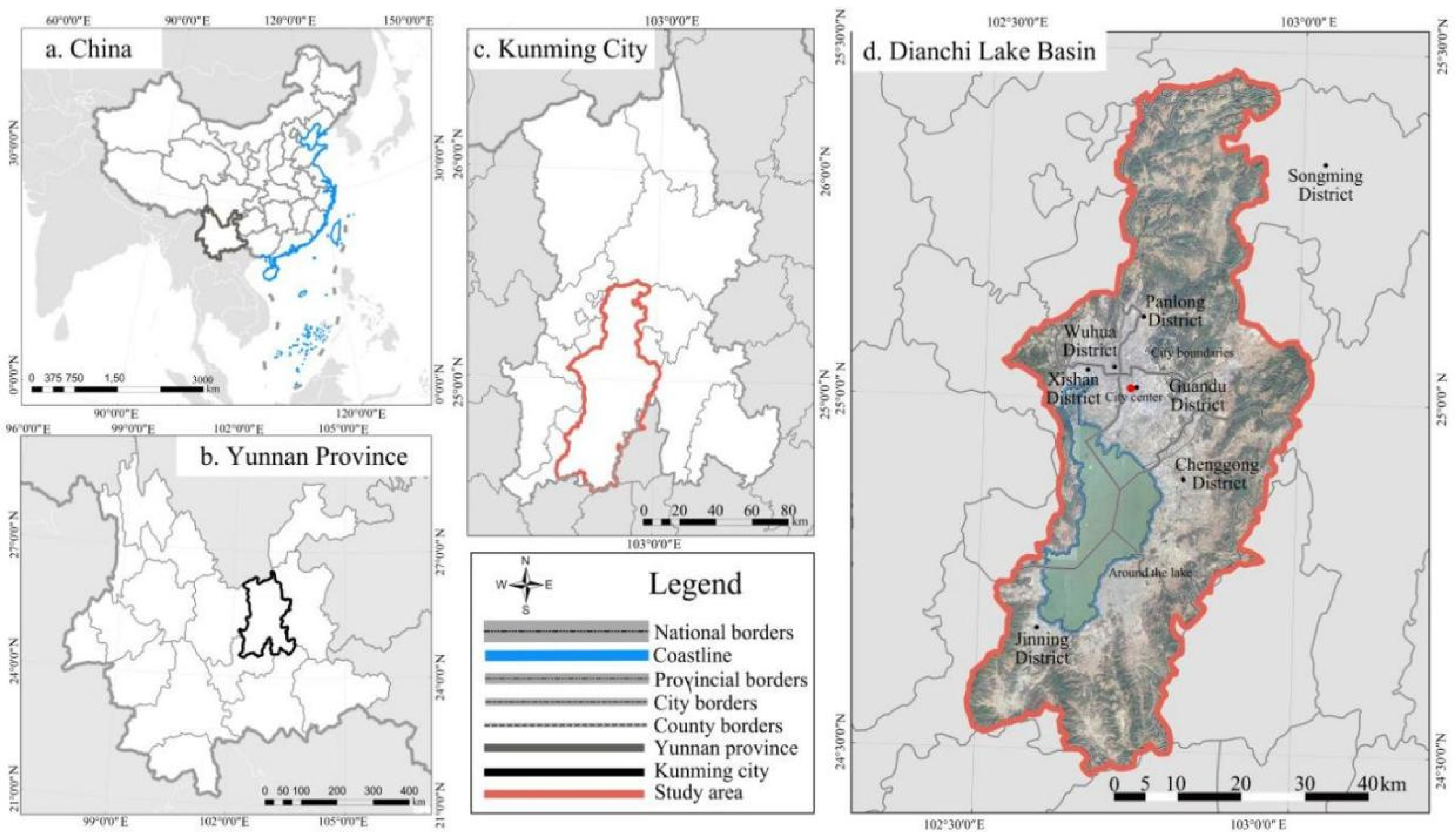
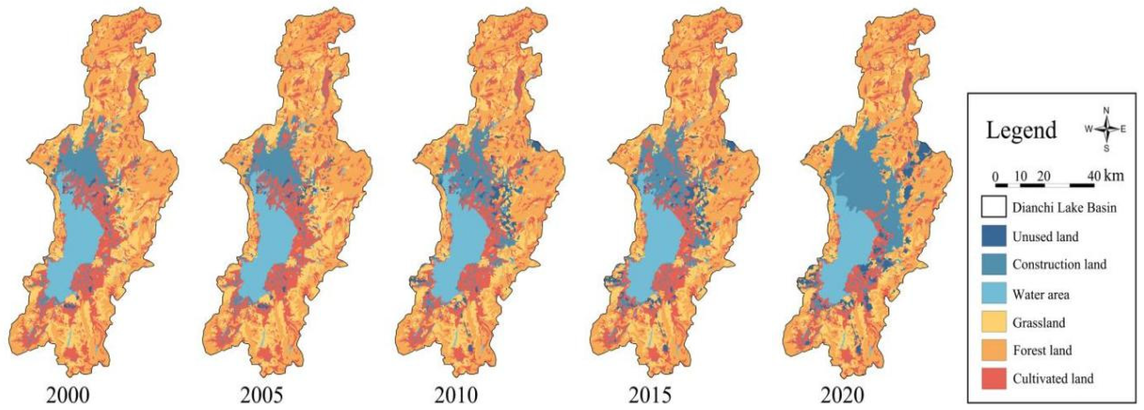
2.1. Study Area

The LDB, covering an area of 2920 km² and representing 3.43% of Yunnan Province, features a subtropical monsoon climate, characteristic of a highland lake region (Figure 1). It has experienced severe water quality degradation and eutrophication over the course of its urbanization and agricultural expansion in the last century [20]. Situated at the core of the Yunnan Central Urban Agglomeration, the LDB occupies 0.7% of Yunnan Province’s total area, hosts 7.6% of the provincial population, and contributes to 24% of the entire province’s GDP. The rapid urbanization and substantial population growth in the 1990s led to the extensive occupation of forested areas, water bodies, and arable land, resulting in habitat destruction for flora and fauna [21]. These issues threaten the ecological balance and sustainable development of the basin, making the study of its ESV crucial for understanding its role in societal and economic contexts and the impact of urbanization.

2.2. Data Sources and Processing

IESV data statistics include three key indicators: (1) LSV based on an empirical model of LULC to reflect human development and disturbance. The LULC data derived from the Resource and Environmental Science Data Registration and Publishing System were validated using a confusion matrix approach [22], with kappa values ranging from 0.93 to 0.96, indicating high accuracy (https://www.resdc.cn/DOI) (accessed on 1 December 2020). (Figure 2) [23]. (2) NPPV generated from the vegetation cover of the LDB, which is an important indicator for evaluating ecosystem services and urban ecological space. Data were sourced from MODIS (https://code.earthengine.google.com/) (accessed on 15 December 2021). (3) CSV to realize changes in the structure of human production was produced from the carbon module of the InVEST model, which simulates timber harvest, harvest product decay, and carbon sequestration in four carbon pools to estimate the carbon sequestration in the current landscape.

LSV, NPP, and CSV all reflect the quality, quantity, and structure of organic matter produced by the ecosystem and are important indicators of China’s ecological compensation policy. This is converted into equivalent energy of standard coal mass to estimate the service value of material production (

Table 1. Data statistics table.

Data Type	Data Sources	Data Time/Year	Resolution/m
Satellite data	Landsat 4–5 TM, Landsat 8 OLI_TIRS, Landsat 8–9 OLI/TIRS C2 L2	2000, 2005, 2010, 2015, 2020	30
Vector data	http://geodata.pku.edu.cn (accessed on 1 December 2020)	2020
LULC	http://www.ncdc.ac.cn/portal/ (accessed on 1 December 2020) https://www.resdc.cn/ (accessed on 1 December 2020) http://www.dsac.cn/ (accessed on 1 December 2020)	2000, 2005, 2010, 2015, 2020	30
Digital elevation	http://geodata.pku.edu.cn (accessed on 1 December 2020)	2020	30
Statistical yearbook data	https://stats.yn.gov.cn/List22.aspx (accessed on 1 December 2020)	2000, 2005, 2010, 2015, 2020

).

2.3. Research Methodology

2.3.1. Single-Factor Accounting of LSV, CSV, and NPPV

(1)

Analysis and calculation of LSV

We calculated the LSV for the LDB using the annual LULC data. The methodology is based on the per unit area equivalent factor table developed by [24] and adjusted for the specific land use conditions of our study area [25]. To mitigate the impact of inflation, LSV was calculated based on 2020 crop prices, yields, and planting areas.

Cultivated land values were determined as the average of dry paddy fields, while forested areas comprised the average values of coniferous forest, mixed coniferous and broadleaf forest; shrubland and grassland values were calculated based on the average of irrigated grassland and natural grassland. Water areas corresponded to the LDB region, and unused land values were computed as the average of wetlands and bare land (

Table 2. LSV equivalent factor table per unit area in the LDB.

Level 1 Type	Level 2 Type	Farmland	Forestry	Grassland	Water Area	Unused Land	Construction Land
Supply services	Food production	1.11	0.25	0.23	0.80	0.01	0.01
	Raw material production	0.25	0.58	0.34	0.23	0.02	0.00
	Water supply	−1.31	0.30	0.19	8.29	0.01	−7.51
Adjust the service	Gas regulation	0.89	1.91	1.21	0.77	0.07	−2.42
	Climatic regulation	0.47	5.71	3.19	2.29	0.05	0.00
	Purify the environment	0.14	1.67	1.05	5.55	0.21	−2.46
	Hydrologic regulation	1.50	3.74	2.34	102.24	0.12	0.00
Support services	Soil conservation	0.52	2.32	1.47	0.93	0.08	0.02
	Maintain nutrients	0.16	0.18	0.11	0.07	0.01	0.00
	Biodiversity	0.17	2.12	1.34	2.55	0.07	0.34
Cultural	Aesthetic landscape	0.08	0.93	0.59	1.89	0.03	0.01

).

The economic value of one equivalent factor is equivalent to 1/7 of the annual average market value of grain yield in the study area [26,27]. To mitigate the impact of inflation, fixed values were determined for grain prices, planting area, and yield. The remaining land use types were treated as variables for scientific estimation. Conclusions were drawn based on a comprehensive investigation of the main grain crops in the study area, utilizing relevant data for rice (Unit Price: 3.55 CNY/kg; Planting Area: 3.01 × 10⁷ ha; Yield: 7044.25 kg/ha), wheat (Unit Price: 2.66 CNY/kg; Planting Area: 2.34 × 10⁷ ha; Yield: 5742.25 kg/ha), and corn (Unit Price: 2.50 CNY/kg; Planting Area: 4.13 × 10⁷ ha; Yield: 6316.97 kg/ha) in 2020 as the main indicators. The formula for calculation is as follows [28]:

$$E_n={\displaystyle \frac{1}{7}}\sum _{i=1}^m{\displaystyle \frac{o_i{p}_i{q}_i}{M}}$$

(1)

In Equation (1), E_n represents the economic value of crop production per unit area in the study area (CNY/ha), where i denotes the type of crop, and oi, p_i, and q_i represent the planting area (ha), yield (kg/ha), and average price (CNY/kg) for crop i, respectively. M is the total planting area for the three crops (rice, wheat, and corn). Ultimately, the calculated value for the economic value per unit area (LSV) in 2020 is 2655.77 CNY/ha. Multiplying this value by the coefficient yields the economic value for different LULC types in the LDB (

Table 3. LSV per unit area of LDB (Units:10⁴ CNY/ha).

Level 1 Type	Level 2 Type	Farm Land	Forestry	Greens Ward	Water Area	Unused Land	Construction Land
Supply services	Food production	0.29	0.07	0.06	0.21	0.00	0.00
	Raw material production	0.07	0.15	0.09	0.06	0.01	0.00
	Water supply	−0.35	0.08	0.05	2.20	0.00	−1.99
Adjust the service	Gas regulation	0.24	0.51	0.32	0.20	0.02	−0.64
	Climatic regulation	0.12	1.52	0.85	0.61	0.01	0.00
	Purify the environment	0.04	0.44	0.28	1.47	0.06	−0.65
	Hydrologic regulation	0.40	0.99	0.62	27.15	0.03	0.00
Support services	Soil conservation	0.14	0.62	0.39	0.25	0.02	0.01
	Maintain nutrients	0.04	0.05	0.03	0.02	0.00	0.00
	Biodiversity	0.05	0.56	0.36	0.68	0.02	0.09
Cultural services	Aesthetic landscape	0.02	0.25	0.16	0.50	0.01	0.00
Total		1.06	5.23	3.21	33.36	0.18	−3.19

Note: The equivalent factor table was adjusted and modified based on previous research and the LULC characteristics of the LDB [24].

).

The calculation formula for LSV is as follows [29]:

$$\mathrm{E}\mathrm{S}\mathrm{V}=\sum _{\mathrm{i}=1}^{\mathrm{n}}({\mathrm{A}}_{\mathrm{i}}\times {\mathrm{V}\mathrm{C}}_{\mathrm{i}})$$

(2)

In Equation (2), A_i represents the area of the ith land type, and VC_i represents the economic value of the ith land type.

(2)

Analysis and calculation of CSV

This study harnessed the carbon module of the InVEST model to comprehensively assess the carbon sequestration functions in the LDB [30]. The InVEST model’s carbon module plays a pivotal role by integrating multiple data sources. It takes into account land use patterns, timber harvest activities, the decay of harvest products, and the carbon stock within four distinct carbon pools: above ground biomass, below ground biomass, soil, and dead organic matter. By leveraging these data, the model is able to estimate the carbon stock in the current landscape.

Functioning at the raster unit level, the model demands a precise estimate of carbon storage within each grid cell across the four fundamental carbon pools. To ensure the model’s accurate performance, the proper setting of parameters in the carbon module is of utmost importance. In this particular study, parameter values were carefully determined by referring to relevant literature and considering the specific characteristics of the study area, as presented in

Table 4. Values of carbon density parameters of different ground categories (Units: t/ha).

Land Use Type	Ci_above	Ci_soil	Ci_below	Ci_dead	Total Carbon
Farmland	6.15	55.60	4.06	0.48	66.29
Forestry	55.17	308.46	11.03	1.10	375.76
Greensward	5.52	28.38	19.33	2.92	56.15
Water	0.00	14.78	0.00	0.00	14.78
Construction land	6.38	22.17	1.28	0.00	29.83
Unused land	0.73	15.35	0.72	2.19	18.99

. The underlying fundamental principles of the model are outlined as follows [31,32]:

$${\mathrm{C}}_{\mathrm{i}}={\mathrm{C}}_{\mathrm{i}-above}{+\mathrm{C}}_{\mathrm{i}-soil}{+\mathrm{C}}_{\mathrm{i}-below}{+\mathrm{C}}_{\mathrm{i}-dead}$$

(3)

In Equation (3), C_i represents the carbon content of the land use type; C_i-above refers to the above-ground carbon density; C_i-soil signifies the carbon content in soil; C_i-below denotes the below-ground carbon accumulation; and C_i-dead indicates the carbon content in dead biomass. The carbon values are converted to units of t/ha before conducting unified calculations. As presented in Table 4, values of carbon density parameters for different ground categories (units: t/ha) were obtained based on previous research [33]. These parameters, including above-ground, below-ground, soil and dead carbon values, are crucial for calculating the total carbon in various land use types, such as farmland, forestry, greensward, water, construction land, and unused land.

(3)

Analysis and calculation of NPPV

NPP data are frequently calculated using the CASA (Carnegie–Ames–Stanford Approach) model [34]. Due to the limitations of the CASA model in this experiment, such as extensive data requirements and difficulty in obtaining precise data, we adopted an alternative approach. We analyzed NPP data interpreted from MODIS satellite imagery available on the NASA official website [35]. Firstly, the original data, which are in units of g.c/m², were multiplied by 1 × 10⁻⁴. Then, to match the resolution of other data used in the study, they were resampled to a 30 m resolution. To ensure unit consistency, we converted the data from g.c/m² to t.c/ha based on the carbon market unit price. Finally, the raster calculator was used to perform the final estimation. This process enabled us to obtain accurate NPPV data for further analysis.

2.3.2. Integrated Evaluation Index System

(1)

CSV and NPPV effective carbon value conversion.

NPP and CSV can reflect the quality of organic matter produced by the ecosystem, so the energy substitution method can be used to quantify the value of ecosystem material production services in the form of NPP and CSV. Carbon storage can also be calculated in this way. On this basis, it is converted into the quality of standard coal with equivalent energy, and the market price of standard coal is used to indirectly estimate the value of material production services.

NPPV and CSV were estimated using a comprehensive carbon unit price of 70.00 USD/t [36,37], referencing

Table 5. CSV and NPPV effective carbon value conversion.

Item	Content	Source
NPP and Carbon Storage Value Estimation Method	Using the energy substitution method, estimating by converting to standard coal quality and using market price	[40]
Standard Coal Price (2020)	CNY 522.22–603.33 CNY/ton (based on market price and heat conversion)	[41,42]
Coal conversion to standard coal prices	Standard coal unit price = Raw coal unit price raw coal quantity/Standard coal quantity	[43]
Calorific Value of Standard Coal	7000 kcal (complete combustion)
Organic Matter to Standard Coal Energy Conversion	1 gC = 1.474 g standard coal	[44]
Afforestation Cost	305 CNY/t (using market price)	[45]
ESV (CNY)	464.43–585.82 CNY/t (after deducting afforestation costs)
ESV (USD)	67.31–84.90 USD/t (converted at 2020 exchange rate)

and the 2020 carbon unit price data from the summary of the Paris Agreement [38,39]. The calculations were converted to 482.82 CNY/t based on the average exchange rate of 6.90 USD in 2020 (https://www.safe.gov.cn/)(accessed on 1 December 2020).

(2)

Evaluation index system.

The integrated evaluation index system was constructed by selecting factors for LSV, NPPV, and CSV. The data for LSV, NPPV, and CSV evaluation factors for the years 2000–2020 were aggregated into five periods. Using the natural breaks classification method (Jenks from ArcGIS 10.8), the data were categorized into two major levels and six sub-levels (

Table 6. Table of the integrated evaluation index system (Units: CNY/ha).

Level		No.	LSV (104)	NPPV (103)	CSV (103)	IESV (×103)
Low- yield areas	Incipient Value	1	−0.33–−0.11	0.56–1.54	0.00	−0.93–0.08
	Emergent Value	2	−0.11–0.10	1.54–2.73	0.00–0.68	0.08–1.38
	Developing Value	3	0.10–0.24	2.73–3.51	0.68–1.16	1.38–2.25
High- yield areas	Elevated Value	4	0.24–0.40	3.51–4.29	1.16–1.69	2.25–3.21
	Advanced Value	5	0.40–0.75	4.29–5.07	1.69–3.26	3.21–5.63
	Peak Value	6	0.75–1.09	5.07–6.98	3.26–6.15	5.63–7.96

).

(3)

Analysis of entropy weight by TOPSIS method.

We applied the entropy-weight method for objective weight determination, analyzing environmental data changes via entropy. This approach identifies the variability and significance of different attributes. Additionally, conversion of the Technique for TOPSIS was utilized to evaluate targets against ideal solutions. Combining these methods, we addressed multi-attribute decision-making in environmental analysis, ensuring a balanced evaluation of each attribute’s weight and importance (

Table 7. Entropy-weight TOPSIS weight calculation panel.

Indicators	LSV	NPPV	CSV
Positive ideal solution	0.36	0.40	0.25
Negative ideal solution	0.01	0.02	0.01
Sum of squares	0.25	0.32	0.06
Optimal distance	0.50	0.56	0.25
Sum of squares	0.21	0.28	0.21
Worst distance	0.46	0.52	0.46
Proximity	0.48	0.48	0.64
Weight	0.29	0.32	0.39

) [46,47]. The TOPSIS method is employed to evaluate targets against ideal solutions, which helps us determine the relative importance of different ESV indicators (LSV, NPPV, and CSV). By calculating the proximity to the ideal solution, we can comprehensively assess the IESV and understand the contribution of each indicator.

2.3.3. Integrated Evaluation Index Spatial Autocorrelation Analysis

Spatial autocorrelation refers to the correlation of the values of a variable within a given spatial distance, and IESV, being a metric for continuous spatial patterns, exhibits spatial correlation. This study employs both global and local Moran’s I indices to measure the spatial clustering degree of IESV variations [48].

Global Moran’s I: This statistic assesses overall spatial dependency across the study area, indicating whether IESV variations are clustered, random, or dispersed. A positive Moran’s I indicates a positive spatial correlation, while a negative value suggests a negative correlation. The closer the Moran’s I value is to 1 or −1, the stronger the spatial correlation. The expression is as follows:

$$I={\displaystyle \frac{n\sum _{i=1}^n\sum _{j=1}^n{W}_{ij}(X_i-\overline{X})(X_j-\overline{X})}{\sum _{i=1}^n\sum _{j=1}^n{W}_{ij}\sum _{i=1}^n{(X_i-\overline{X})}^2}}$$

(4)

In Equation (4), n represents the sample size. X_i and X_j denote the IESV (variations) at locations i and j within the region, respectively. $\overline{\mathrm{X}}$ is the mean of the samples. W_ij is the spatial weight matrix. The Moran’s I is within the [−1, 1] range. A positive Moran’s I is a positive spatial correlation, while a negative Moran’s I is a negative spatial correlation. The closer the absolute value of I is to 1, the stronger the correlation.

Local Moran’s I: This measure identifies local spatial autocorrelation patterns in IESV, providing insight into how land use intensity clusters at specific locations. A positive local Moran’s I indicates clustering of similar values (high–high or low–low), whereas a negative value indicates a high–low or low–high pattern. The expression is as follows:

$$I={\displaystyle \frac{\sum _{j=1,j\ne i}^n{W}_{ij}(X_i-\overline{X})(X_j-\overline{X})}{\sum _{i=1}^n{(X_i-\overline{X})}^2}}$$

(5)

2.3.4. COG (Center of Gravity) Analysis

The barycenter refers to a certain spatial point, in which the powers are relatively balanced in all directions. As an important analysis tool for studying changes of spatial patterns, barycenter models, such as the grain production barycenter model, the population barycenter model, and the energy barycenter model, are also frequently used for spatial analysis. The ecological service value barycenter is formed according to the above theory. The barycentric coordinates can be calculated by the following formula [49]:

$$x_j=\sum _{i=1}^n(T_{ij}·x_i)/\sum _{i=1}^n{T}_{ij}$$

(6)

$${\mathrm{y}}_j=\sum _{i=1}^n(T_{ij}·y_i)/\sum _{i=1}^n{T}_{ij}$$

(7)

where T_ij (i = 1, 2, 3, … n) means the grain output of the ith county; P_i (x_i, y_i) is the barycentric coordinate of each county; and Pj (x_j, y_j) is the national barycentric coordinate of grain output in the jth year.

2.3.5. CA-MC Model Prediction Analysis

This section discusses the integration of the Cellular Automata (CA) model and the Markov Chain (MC) model for predicting spatial-temporal dynamics in the LDB. CA Model: The CA model is characterized by its components: cells, cell space, neighborhoods, and transition rules. It operates on discrete and finite states in time, space, and status, applying synchronous transitions based on local rules. The model is defined as follows [50]:

S = (t + 1) = f [S(t), N]

(8)

In Equation (6), S represents a finite and discrete state set of cells; N represents the neighborhood of cells; and f is the local mapping for the cellular transition rule.

MC Model: The MC model calculates spatial transition probabilities, interpreting temporal patterns of change in various states. It is essential for time series analysis, predicting transitions based on probability matrices, expressed as follows [51]:

N_t+1 = N_t × P_ij

(9)

$$\begin{array}{c}{\mathrm{P}}_{\mathrm{ij}}=\left[\begin{array}{ccc}{\mathrm{P}}_{11}& \begin{array}{cc}{\mathrm{P}}_{12}& \dots \end{array}& {\mathrm{P}}_{1\mathrm{n}}\\ {\mathrm{P}}_{21}& \begin{array}{cc}{\mathrm{P}}_{22}& \dots \end{array}& {\mathrm{P}}_{2\mathrm{n}}\\ \begin{array}{c}⋮\\ {\mathrm{P}}_{\mathrm{n}1}\end{array}& \begin{array}{cc}\begin{array}{c}⋮\\ {\mathrm{P}}_{\mathrm{n}2}\end{array}& \begin{array}{c}\dots \\ \dots \end{array}\end{array}& \begin{array}{c}⋮\\ {\mathrm{P}}_{\mathrm{n}\mathrm{n}}\end{array}\end{array}\right]\\ 0 \le {\mathrm{P}}_{\mathrm{ij}} < 1 \mathrm{AND}\sum _{\mathrm{j}=1}^{\mathrm{n}}{\mathrm{P}}_{\mathrm{i}\mathrm{j}}=1(\mathrm{i},\mathrm{j}=1,2\dots ,\mathrm{n})\end{array}$$

(10)

In Equations (7) and (8), N_t+1 represents the LULC classification in the subsequent time period, N_t represents the LULC classification in the previous time period, and P_ij denotes the state transition probability matrix.

CA-MC Integration: Combining the CA and MC models leverages the strengths of both, enabling robust predictions of IESV changes [52]. The Kappa coefficient evaluates prediction accuracy:

$$\mathrm{Kappa}=({\mathrm{P}}_0-{\mathrm{P}}_{\mathrm{c}})/({\mathrm{P}}_{\mathrm{p}}-{\mathrm{P}}_{\mathrm{c}})$$

(11)

In Equation (9), P₀ represents the proportion of accurately simulated outcomes, P_c denotes the proportion of correct predictions under random model conditions, and P_p indicates the proportion of correctly predicted outcomes under ideal conditions.

The CA-MC model is used to predict the spatiotemporal dynamics of IESV. The CA model, with its components of cells, cell space, neighborhoods, and transition rules, can simulate the local and synchronous changes of ESV. The MC model calculates the spatial transition probabilities, which is essential for analyzing the temporal patterns of change. Combining these two models allows us to project future trends of IESV in the LDB, providing valuable information for sustainable urban planning.

3. Results and Analysis

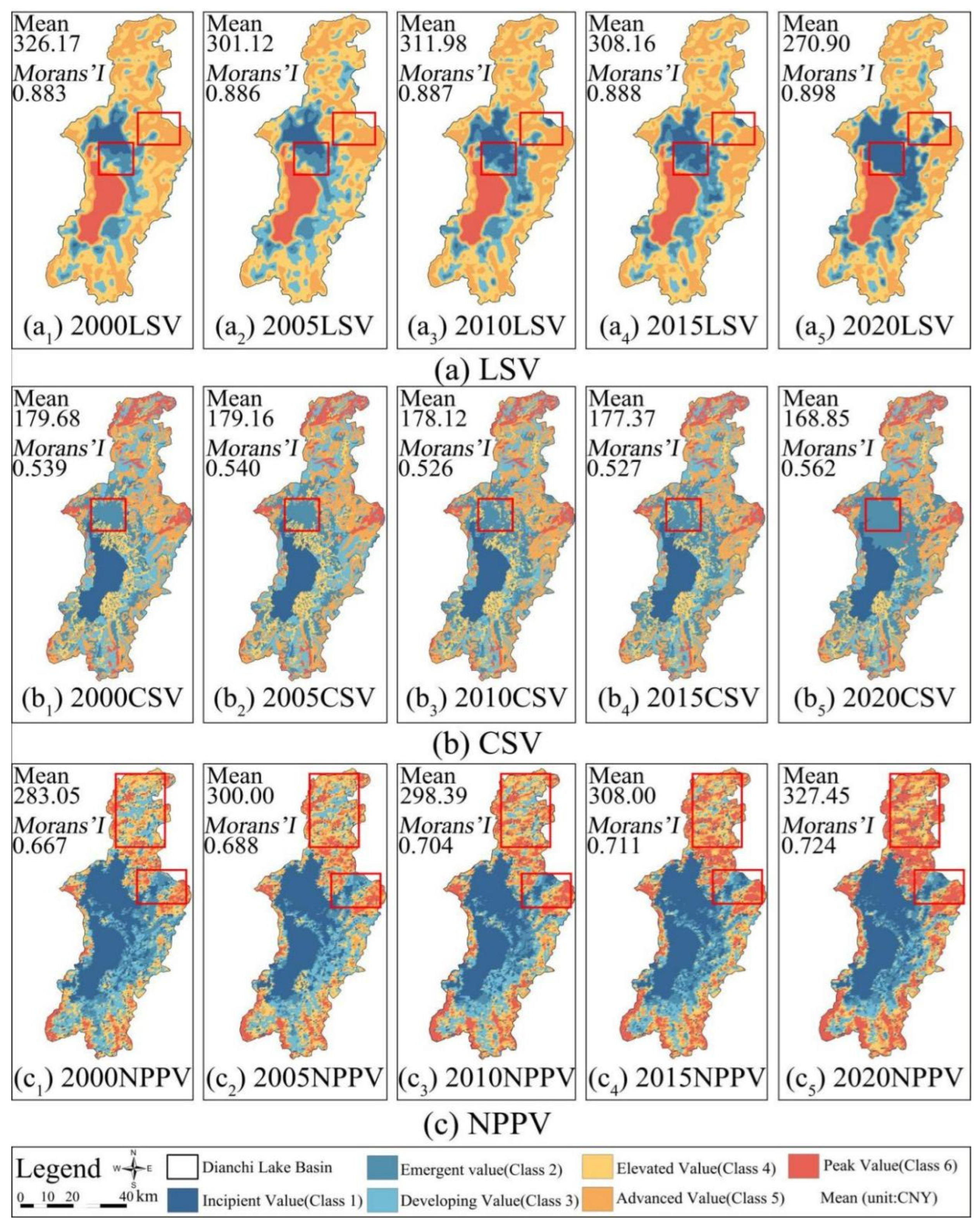
3.1. Distribution Characteristics of LSV, CSV, and NPPV

Over the two-decade period from 2000 to 2020, our analysis revealed distinct spatial and temporal patterns in the distribution of LSV, CSV, and NPPV within the LDB. Lake Dianchi emerged as a key area in LSV, characterized by high output levels attributable to its substantial water resource reserves. In contrast, CSV and NPPV primarily highlighted terrestrial ecosystem productivity in high-yield zones near urban peripheries, which were observed to be expanding over time.

The response of LSV, CSV, and NPPV to urban expansion was evident. As urban areas expanded, low-value zones around urban centers and their adjacent lands became more pronounced, expanding over time yet not dominating in any accounting system. In contrast, CSV and NPPV were predominantly characterized by small patchy landscape structures within the same region, displaying a heterogeneous mix of peak value, advanced value, and emergent value states. Over multiple years of CSV and NPPV data, the high-production areas were clustered along the northern and eastern edges of the study area, and most of them were located in montane forested areas. Statistical analysis confirmed a significant decline in LSV over 20 years (R² = 0.89, p < 0.01), while NPPV increased by CNY 44.4. The period from 2015 to 2020 marked notable changes; LSV and CSV reached their lowest values in 2020, decreasing by CNY 37.26 and CNY 8.52, respectively, and NPPV peaked at CNY 327.45 (Figure 3).

3.2. Analysis of Structural Trend Characteristics of LSV, CSV, and NPPV

We categorized the six value areas (Classes 1 to 6) into two groups: high-yield (Classes 4, 5, and 6) and low-yield (Classes 1, 2, and 3) areas. By examining the transformation and spatial transfer characteristics across these areas, we delved into the change and contribution of LSV, CSV, and NPPV (Figure 4). LSV followed a normal distribution, with smaller areas corresponding to extreme outputs (either very high or very low) and larger areas with moderate output. This pattern indicates a stable and consistent systemic trend (Figure 4(a1)). Over the years, LSV initially experienced a decline, followed by a period of slow increase, ultimately leading to an overall steady decline, particularly after 2015; CSV predominantly exhibits a bimodal distribution, suggesting the presence of two distinct groups or distributions within the data. The low-output CSV peak primarily includes water and urban areas, while the high-output peak comprises green spaces and shrubbery. This pattern indicates a mix of separation and partial integration within the system. Over time, CSV showed a gradual decrease, with a marked decline after 2015 (Figure 4(a2)); NPPV shows a U-shaped distribution, with signs of human influence. This may be due to natural and anthropogenic factors. Naturally, the subtropical monsoon climate and mountainous topography help forests grow in high-altitude rainy areas, increasing NPPV at the high-output end. Urbanization first reduces NPPV by clearing vegetation but later raises it through greening. Intensive farming can lower NPPV by degrading soil, while sustainable practices can increase it. Polluting industries decrease NPPV, and green-tech-investing industries can boost it. From 2000 to 2020, NPPV grew overall, peaking in mid-output areas and increasing by 1.51 (10⁸ CNY). It changed less than LSV and CSV from 2010 to 2015 but diverged significantly after 2015 (Figure 4(a3)).

In terms of long-term changes, land area evaluations showed a continual expansion of low-yield areas, especially around urban centers. From 2000 to 2020, a significant shift was observed in LSV from high-yield to low-yield areas, encompassing 26,152.60 ha (8.52% of the total area). Similarly, CSV also exhibited a notable transition of 16,549.55 ha (5.40% of the total area) from high to low yield. Granted, the transition of high-value area coverage to low-value areas also led to a decline in ecological service value. From 2000 to 2020, LSVs and CSVs decreased by 1.88 (10⁸ CNY) and 0.37 (10⁸ CNY), respectively, indicating an overall downward trend (Figure 4). However, NPPV displayed an opposite trend, with minimal changes in the lowest-yielding areas and significant expansion in high-yield regions. This expansion led to an increase in NPPV by 1.51 (10⁸ CNY), demonstrating an overall upward trend. Overall, this evidence suggests that LSV and CSV are significant contributors to the multi-year decline in ESV in the LDB (Figure 4b).

Spatial transition analysis revealed that 65% of the low-yield zone expansion occurred in former agricultural lands converted to urban areas, corroborating the impact of urbanization. These region-wide dynamics are expressed in the equilibrium analysis of spatial development as a shift in the COG. The COG analysis reflects the spatial distribution and movement of LSV, CSV, and NPPV over the study period. From 2000 to 2020, the centroids of all three factors migrated southward, with NPPV experiencing the greatest shift (2.504 km southeast), followed by LSV (2.01 km southeast), and CSV (0.511 km southeast). This southward trend in the LDB indicates a relatively even development, with a notable increase in spatial COG movement post-2015 (Figure 4c). Spearman’s rank correlation confirmed a significant southeastward trend in COG migration (R² = 0.91, p < 0.001).

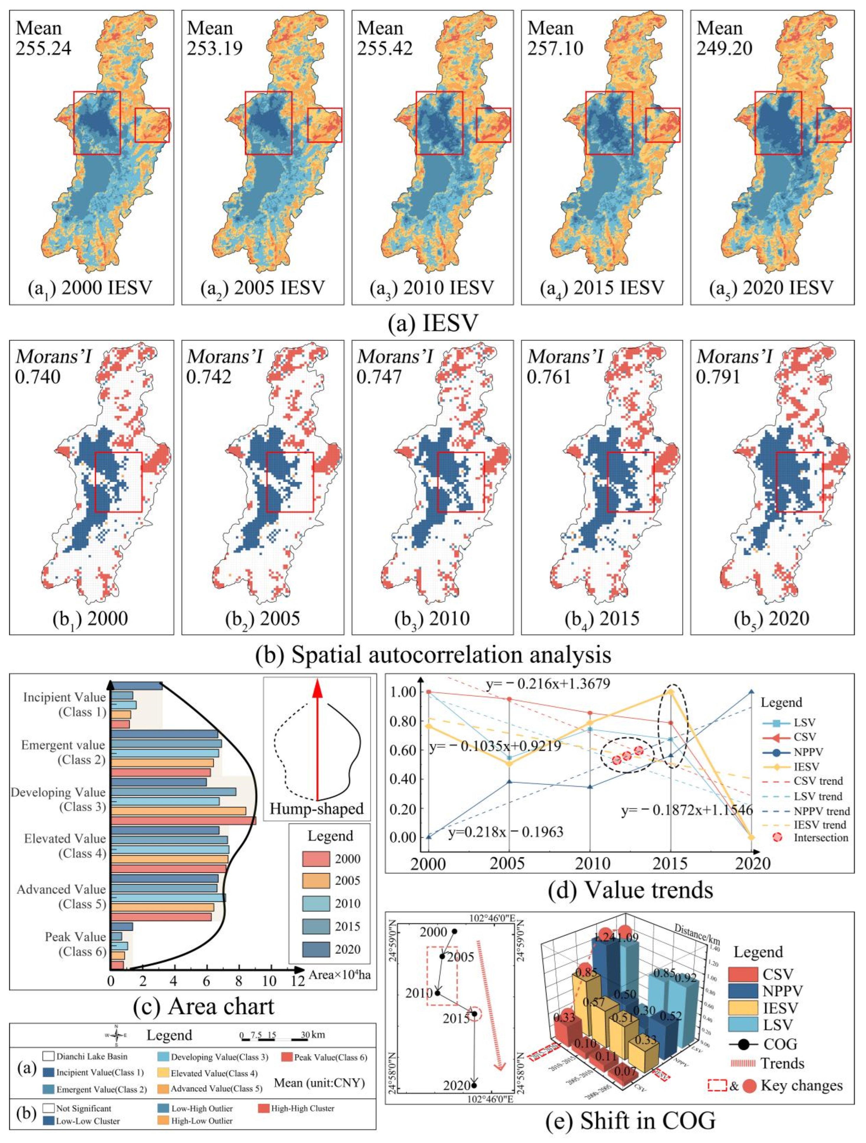
3.3. IESV Spatiotemporal and Quantitative Change Characteristics

In the comprehensive assessment of IESV, we observed that while the spatial distribution of high- and low-output areas remained essentially stable (Figure 5(a1)–(a5)), there was a slight increase in their degree of aggregation (Figure 5(b1)–(b5)). Specifically, within the low-yield zones, a pronounced trend of output expansion centered around urban areas was evident. This trend is reflected in the Moran’s I cluster analysis, where the Low–Low (LL) clustering area progressively expanded, leading to the formation of more extensive low-yield regions across the study area (Figure 5b).

From the perspective of data structure, the results increasingly aligned with a normal distribution, integrating features from both LSV and CSV structures. Compared to LSV and CSV, NPPV’s influence, albeit limited, suggested a compensatory effect that could slow down the IESV decline, yet it was insufficient to reverse the overall downward trend. The Incipient Value and Peak Value areas were relatively small, with other regions being larger and more uniformly sized, indicating system stability (Figure 5c).

Concurrently, there was a modest increase in the number of high-yield regions. Throughout the study period, an area of 5792.06 ha transitioned from low to high yield, representing 1.89% of the total area. However, it is important to note that the patchy spatial distribution characteristic of high-yield areas remained relatively unchanged. In the period from 2000 to 2020, the area for both the lowest (Class 1) and highest yield (Class 6) categories in the IESV did not exceed 40,000 hectares annually. The dispersed distribution of high-yield areas somewhat limited their ecological benefits. In terms of productivity, from 2000 to 2020, the IESV decreased by 0.21 (10⁸ CNY), with a trend slope of −0.1035, indicating a downward trend (Figure 5d).

From 2000 to 2020, the COG of IESV generally migrated southeastward, with two southwestward shifts during 2000–2005 and 2005–2010, and a subsequent southeastward movement from 2010. This coincided with significant urban development in Kunming, expanding from the northwest of Lake Dianchi to the southeast. The movement of the municipal government to Chenggong District resulted in considerable land use changes. The southeastward migration of IESV between 2015 and 2020 is hypothesized to be influenced by policy or human interventions. The COG migration distance of IESV, compared to individual factors such as LSV, CSV, and NPPV, was moderate, indicating a relative stability of the overall IESV after comprehensive accounting (Figure 5).Visual interpretation of spatial maps (Figure 5) identified the northern and eastern outskirts of Kunming as hotspots of NPPV growth, driven by afforestation policies. Conversely, the urban core and north shore of Lake Dianchi emerged as degradation hotspots due to urban sprawl.

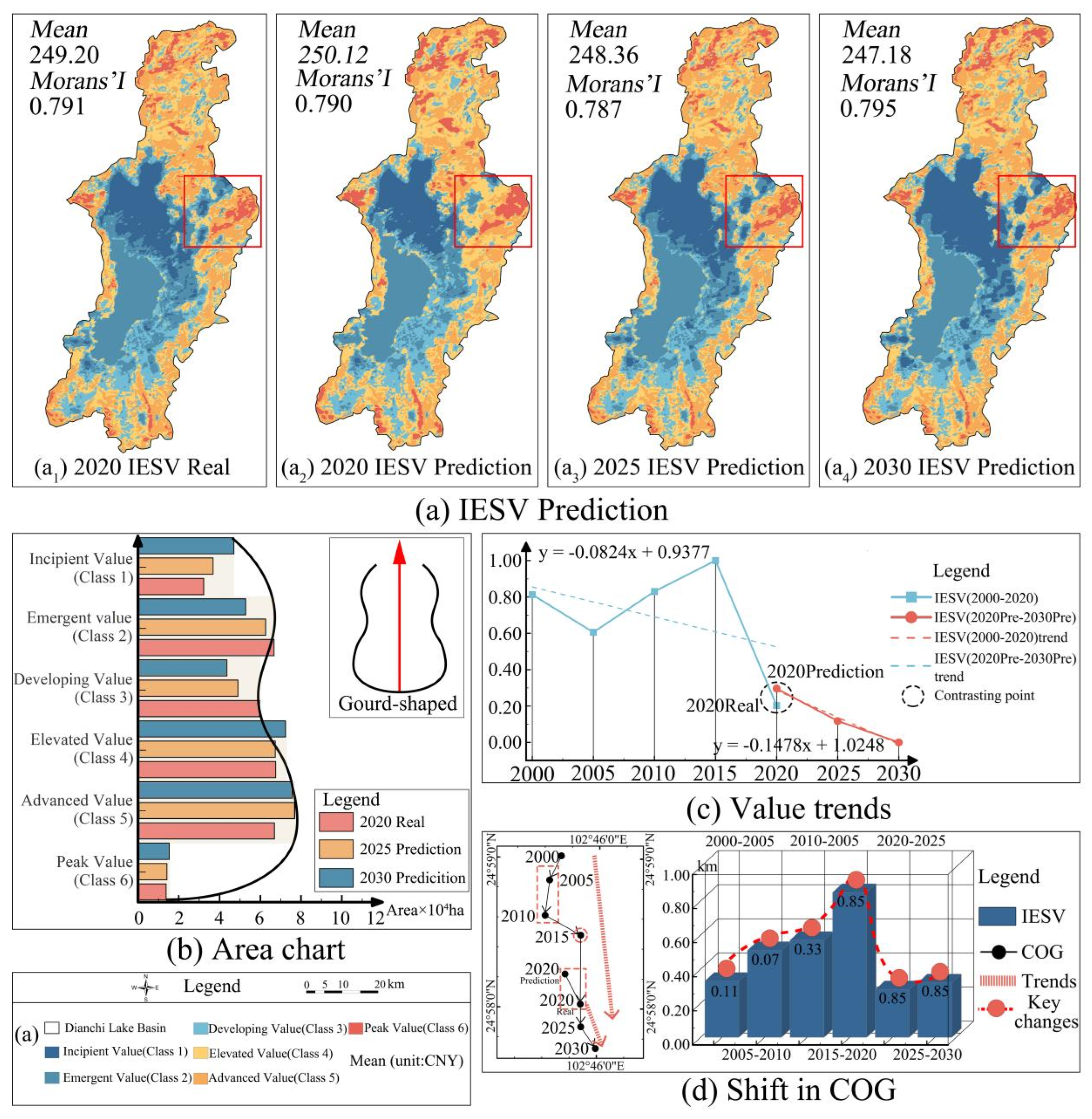
3.4. IESV Spatiotemporal Prediction Based on CA-MC Model

The CA-MC model simulation exhibited robust predictive capabilities, as indicated by a Kappa coefficient of 0.81. Utilizing this model, we projected the IESV changes for the study area for 2025 and 2030. The forecast, as presented in Figure 6, anticipates that about 150.32 km² will shift from low-yield to high-yield zones over the next decade, representing 4.90% of the total area. The projected IESV values expected to show a marginal decline, estimating 8.47 (10⁸ CNY) and 8.43 (10⁸ CNY) for 2025 and 2030, respectively, compared to 2020’s value (Figure 6).

We assessed the 2020 IESV predictions against actual data (

Table 8. Accurate IESV forecast, 2020.

Level		Actual Raster	Prediction Raster	Forecast Consistency	Accuracy (%)
Low-yield areas	Incipient Value	357,252	305,111	280,620	78.55
	Emergent Value	740,866	660,016	483,968	65.32
	Developing Value	552,065	582,026	444,173	80.46
High-yield areas	Elevated Value	748,962	919,800	620,022	82.78
	Advanced Value	854,721	698,121	514,667	60.21
	Peak Value	153,038	240,596	115,979	75.78

). The predicted average value for 2020 was slightly higher at 250.12, against the actual value of 249.20, resulting in a negligible error of 0.37%. Spatially, the low-yield areas (Classes 1, 2, and 3) were projected to intensify their spatial aggregation around Kunming from 2020 to 2030 (Figure 6a).

The IESV predictions again displayed a bimodal distribution, mirroring the spatial distribution pattern of CSV. Notably, as seen in Figure 6b, the data’s dual peaks are shifting towards more pronounced low–high extremes compared to CSV. Despite an increase in high-yield areas (Classes 4, 5, and 6), the overall value was projected to decrease, highlighting the inefficiency in ESV production in fragmented landscapes. Spatial analysis (Figure 6(a₁–a₄) suggests that the mismatch between natural system outputs and human interventions was a significant contributor to this trend. Therefore, the overall value is anticipated to decrease slightly, in line with area changes. The average value prediction for 2030 shows a decrease of CNY 2.02 from 2020’s actual value, with the total IESV decreasing by 0.07 (10⁸ CNY) and a trend slope of −0.1443, indicating a continuous downward trend.

The COG migration trend from 2020 to 2030 is projected to maintain its southeastward trajectory, as shown in Figure 6d. This phase, however, did not exhibit the sharp increase in COG distance noted from 2015 to 2020. The predicted COG migration distance from 2020 to 2023 was 0.992 km, whereas the distance from the actual 2020 to the predicted 2023 was 0.578 km, denoting a relatively stable change. After 2015, the gradual increase in NPPV is anticipated to mitigate the negative impacts of the continuous decline in LSV and CSV (Figure 6d).

4. Discussion

4.1. IESV Changing Trend and Land Efficiency

According to the characteristics of urban development, we integrated key indicators LSV, NPPV, and CSV using weighted overlay analysis to predict IESV trends in the LDB and observed a fluctuating pronounced downward trend in IESV, influenced by the interplay of these indicators.

(1) LSV and CSV Indicators: LSV and CSV indicators showed a phased decline over multiple years. LSV focuses on the impact of land use changes on ecosystem services [53], while CSV is concerned with the carbon storage value in soil and vegetation [54]. These declining trends reflect significant losses in the ESV of the LDB due to LULC during the process of urbanization. (2) NPPV Indicator: In contrast, the NPPV indicator, highlighting vegetation growth and carbon sequestration, showed an upward trend, indicating efforts in ecological conservation [55]. However, the increase in NPPV was insufficient to fully counterbalance the negative impacts of urbanization.

Each indicator represents distinct aspects of ES. LSV represents circulating capital, the value of which was directly circulated and traded in the market [56]; CSV represents fixed assets that exist as reserve value [57]; and NPPV reflects potential profits. Potential development value [58] collectively determines the overall efficiency of ESV production. The declining trends in LSV and CSV primarily indicate consumption in ES, whereas NPPV signifies potential growth. The interplay of these sub-indicators, with gains in one compensating for losses in another, collectively determines that the overall production efficiency of ESV in the current state is at a relatively low level [59].

Related research suggests that the rise of NPP may be an unclear indicator of ecological value in this system. Firstly, the development of the forestry industry is largely driving the increase of NPP, and current regional forestry practices are not ideal for increasing ecological function and value. As of 2020, Kunming’s forestry output value accounted for 4.17% of the agricultural output value. The forestry industry’s early planting investment will face difficulties in the future [60]. Secondly, in the past ten years, relevant ecological protection policies such as returning farmland to forest and grassland have been actively implemented, so that cultivated land, forestland, and grassland receive corresponding vegetation carbon sink compensation. However, policy volatility has been relatively large, and the effectiveness of these incentives on increasing ecological value is uncertain [61]. In summary, the majority of the area in the LDB comprises transitional value zones, with extreme value zones being minimal. Despite shifts in LSV, CSV, and NPPV areas, IESV continues to show a declining trend overall.

These trends are consistent with the MA (Millennium Ecosystem Assessment) framework. The decline in LSV and CSV indicates the degradation of provisioning and regulating services as a result of urbanization, which is in line with the MA’s warning about the negative impacts of urban expansion on ecosystem services [62]. The increase in NPPV, although not enough to offset the overall decline, reflects the positive impact of ecological conservation efforts, similar to the concept of nature-based solutions emphasized by TEEB (The Economics of Ecosystems and Biodiversity) [63]. This shows the complex relationship between urban development and ecosystem services, and the need for a more comprehensive approach to ecosystem management.

4.2. Land Use Comprehensive Assessment

IESV analysis involves spatial dynamics and distribution considerations, especially COG migration. The study showed that the COG of IESV in the LDB remained relatively stable over the past two decades, slowly shifting from north to south. The individual factor characteristics exhibit similar patterns, primarily showing fluctuations between 2005 and 2015. The relative stability of COG may indicate that ecosystem services remain relatively spatially balanced [64]. The migration trend aligns with the spatial trends in the construction of land around Lake Dianchi during this decade, reflecting a gradual southward development along the western shore of Lake Dianchi [65].

The COG is situated in an incipient value area, within the urban core, indicating the spatial distribution of ES (Ecosystem Service) with the city center as the focal point, forming a concentric geometric graph. The overlap of developing value areas with the urban region affects people’s perception of ESV because of misallocation and wastage of green resources. In turn, this gives rise to conflicts between ecological and landscape values.

In 2020, high-value and low-value areas had roughly equal areas, but their spatial clustering characteristics exhibited significant differences. Scattered high-value areas presented small and patchy distributions, characterized by high fragmentation and low connectivity. These fragmented elevated value areas, being small and dispersed, may be unable to provide complete ES compared to large communities and their carbon storage. In contrast, developing value areas aggregate, forming large patches around Lake Dianchi and the urban core, showcasing higher connectivity and more robust internal spatial flow, resulting in more stable ecological impacts.

Therefore, for the entire ecosystem, with equal areas, the negative external impact of developing value areas was more pronounced and should not be overlooked. Our future research focus will be on further verifying the influence of each index on ESV and the relationship between the ecological network and ES in the LDB, including the composition of the network, how ES functions are delivered throughout the network, and the ESV transfer of services [66].

In the previous 20 years, urban development in Kunming expanded continuously from the north to the south shore of Lake Dianchi, including government office relocation and large-scale construction of infrastructure around the lake. During the 2000–2020 period, the overall southward shift in the COG of IESV aligns with trends in related policies and urban development processes over the past two decades. Fortunately, ecological protection has been consistently integrated with urban development, as evidenced in this study by the sustained increase in NPPV. Practically, this is reflected in the expansion of green spaces around the lake and the improvement of the LDB landscape [67].

This situation also reflects the concepts in the MA and TEEB. The MA emphasizes the importance of maintaining the balance of different ecosystem services and the impact of spatial distribution on ecosystem functions. The uneven distribution of high-value and low-value areas in the LDB indicates a potential imbalance in ecosystem services. TEEB’s perspective on the economic value of ecosystem services can help us understand the trade-offs in land use. For example, the aggregation of developing value areas may have economic benefits in the short-term, but it also brings negative ecological externalities. Therefore, when formulating land use policies, it is necessary to consider the long-term impact on ecosystem services and biodiversity.

4.3. Future-Based IESV System Stability

The proportion of incipient value areas in 2020 was relatively low, presenting an overall pattern resembling a normal distribution. However, from 2015 to 2020, there has been a preliminary upward trend in the proportion of incipient value areas. The rise in the incipient value areas of ESV may have implications for the overall stability of the region. On one hand, the increase in incipient value areas may signify an escalation in environmental stress, such as rapid declines in critical ecosystem function indicators, thereby affecting the overall environmental health of the region. On the other hand, the overlap of incipient value areas with urban zones could result in misallocation and wastage of green resources, leading to an overall reduction in ecosystem services, impacting the quality of life for residents and the region’s sustainable development [68]. The simulation results suggest that the continuous increase in extremely low values may persist for an extended period, with the incipient value areas likely experiencing rapid growth between 2020 and 2030. On one hand, the simulation aligns with the existing trend; on the other hand, the CA simulation exhibits characteristics of block-based expansion in their original locations. Due to their clustering nature, low-value areas often demonstrate higher growth rates when expanding at the periphery.

Therefore, the increasing proportion of low-productivity zones in the ESV of the LDB not only further diminishes the efficiency of ecosystem services but also exacerbates the uneven distribution of resources, ecosystem services, or biodiversity within the system. The rise in low-productivity zones, notably in incipient value regions forming large patches, can engender adverse impacts on the overall system value, consequently diminishing the stability of the entire system. This shift is likely associated with factors such as rapid urbanization, adjustments in environmental policies, and climate change within the region, reflecting the sensitivity and dynamic nature of ESV in the face of multiple pressures.

In light of these observations, this shift underscores the critical need for future environmental management and policy formulation. It emphasizes the importance of addressing the stability and sustainability of ESV, recognizing the intricate interplay between ecological changes, urbanization dynamics, and policy interventions. This insight serves as a valuable guide for navigating the complexities of managing ecosystem services amid evolving environmental conditions.

From the perspective of the MA and TEEB, this trend is a warning sign. The MA emphasizes the importance of maintaining the stability of ecosystem structures and functions. The increase in low-productivity zones may lead to a breakdown of the ecosystem structure, affecting its ability to provide services. TEEB’s economic analysis can help us understand the cost of this instability. For example, the loss of ecosystem services may lead to increased costs for environmental protection and restoration. Therefore, future policies should focus on enhancing the stability of ESV, such as promoting sustainable land use and strengthening ecological protection measures.

5. Conclusions

There are certain differences in the assessment of ecosystem service value, which requires us to consider multiple aspects. In our study, three indicators, namely LSV, CSV, and NPPV, were used for overlay analysis to obtain IESV, which can make up for the insufficient explanatory power of a single factor. The phenomenon of urban expansion in the LDB continues to occur. Taking into account the three aspects of landscape, vegetation, and carbon services comprehensively can reflect the correlation between urban spatial development and the spatial and temporal changes of IESV. When LSV and CSV decrease, NPPV increases correspondingly, indicating that afforestation can largely make up for the loss of ESV. Therefore, the purpose of this study is to verify the circularity of various factors of ecosystem services, so as to construct a sustainable development path and improve and enhance the well-being of the human settlement environment through the corresponding measures of relevant departments. However, this study still has some limitations. The indicators we selected have certain errors in data processing and analysis. In the future, integrated analysis and processing methods will be studied in this field to conduct demonstrations from a more scientific and objective perspective.

References

1. Zhang, Y.; Hu, X.; Wei, B.; Zhang, X.; Tang, L.; Chen, C.; Wang, Y.; Yang, X. Spatiotemporal exploration of ecosystem service value, landscape ecological risk, and their interactive relationship in Hunan Province, Central-South China, over the past 30 years. Ecol. Indic. 2023, 156, 111066. [Google Scholar] [CrossRef]
2. Chen, Z.; Zhang, X. Value of ecosystem services in China. Chin. Sci. Bull. 2000, 45, 870–876. [Google Scholar] [CrossRef]
3. Robert, C.; Ralph, d’.A.; Rudolf, d.G.; Stephen, F.; Monica, G.; Bruce, H.; Marjan, B. The value of the world’s ecosystem services and natural capital. Nature 1997, 387, 253–260. [Google Scholar] [CrossRef]
4. Engdaye, M.; Sileshi, D.; Mekuria, A.; Wondimagegn, M. Impact of Land Use Land Cover Changes on Ecosystem Service Values: Implication for Landscape Management. J. Landsc. Ecol. 2025, 18, 61–85. [Google Scholar] [CrossRef]
5. Feng, X.; Huang, H.; Wang, Y.; Tian, Y.; Li, L. Identification of Ecological Sources Using Ecosystem Service Value and Vegetation Productivity Indicators: A Case Study of the Three-River Headwaters Region, Qinghai-Tibetan Plateau, China. Remote Sens. 2024, 16, 1258. [Google Scholar] [CrossRef]
6. Walther, F.; Barton, D.N.; Schwaab, J.; Kato-Huerta, J.; Immerzeel, B.; Adamescu, M.; Andersen, E.; Coyote, M.V.A.; Arany, I.; Balzan, M.; et al. Uncertainties in ecosystem services assessments and their implications for decision support-A semi-systematic literature review. Ecosyst. Serv. 2025, 73, 101714. [Google Scholar] [CrossRef]
7. Dushkova, D.; Konstantinova, A.; Matasov, V.; Gaeva, D.; Dovletyarova, E.; Taherkhani, M. Urban ecosystem services research in Russia: Systematic review on the state of the art. Ambio 2024, 54, 1–26. [Google Scholar] [CrossRef]
8. Guo, Y.; He, P.; Chen, P.; Zhang, L. Ecological Evaluation of Land Resources in the Yangtze River Delta Region by Remote Sensing Observation. Land 2024, 13, 1155. [Google Scholar] [CrossRef]
9. Zhang, L.; Zhang, M.; Guo, Y. Entropy-Weighted TOPSIS-Based Ecological Environment Driving Factors in the Chaohu Lake Rim Region Temporal and Spatial Differentiation Study. Pol. J. Environ. Stud. 2024, 33, 5459–5471. [Google Scholar] [CrossRef]
10. Pourebrahim, S.; Mokhtar, M.B. Conservation priority assessment of the coastal area in the Kuala Lumpur mega-urban region using extent analysis and TOPSIS. Env. Earth Sci. 2016, 75, 348. [Google Scholar] [CrossRef]
11. Mirli, A.; Bakas, T.; Latinopoulos, D.; Kagalou, I.; Spiliotis, M. Participatory Management of a Mediterranean Lagoon Complex Social-Ecological System Using Intuitionistic Fuzzy TOPSIS. Sustainability 2024, 16, 10647. [Google Scholar] [CrossRef]
12. Du, H.; Zhao, L.; Zhang, P.; Li, J.; Yu, S. Ecological compensation in the Beijing-Tianjin-Hebei region based on ecosystem services flow. J. Environ. Manag. 2023, 331, 117230. [Google Scholar] [CrossRef] [PubMed]
13. Zhang, Z.; Li, J.; Lu, Y.; Yang, L.; Hu, Z.; Li, C.; Yang, X. Temporal and spatial changes in land use and ecosystem service value based on SDGs’ reports: A case study of Dianchi Lake Basin, China. Environ. Sci. Pollut. Res. 2023, 30, 31421–31435. [Google Scholar] [CrossRef] [PubMed]
14. Wang, G.; Cushman, S.A.; Wan, H.Y.; Li, H.; Szabó, Z.; Ning, D.; Jombach, S. Ecological Connectivity Networks for Multi-dispersal Scenarios Using UNICOR Analysis in Luohe Region, China. J. Digit. Landsc. Archit. 2021, 10, 230–244. [Google Scholar] [CrossRef]
15. Atesoglu, A.; Ayyildiz, E.; Karakaya, I.; Bulut, F.S.; Serengil, Y. Land cover and drought risk assessment in Türkiye’s mountain regions using neutrosophic decision support system. Env. Monit Assess. 2024, 196, 1046. [Google Scholar] [CrossRef]
16. Yin, Z.; Feng, Q.; Zhu, R.; Wang, L.; Chen, Z.; Fang, C.; Lu, R. Analysis and prediction of the impact of land use/cover change on ecosystem services value in Gansu province, China. Ecol. Indic. 2023, 154, 110868. [Google Scholar] [CrossRef]
17. Li, G.; Cheng, G.; Liu, G.; Chen, C.; He, Y. Simulating the Land Use and Carbon Storage for Nature-Based Solutions (NbS) under Multi-Scenarios in the Three Gorges Reservoir Area: Integration of Remote Sensing Data and the RF-Markov-CA-InVEST Model. Remote Sens. 2023, 15, 5100. [Google Scholar] [CrossRef]
18. Xia, X.; Shirong, Q.; Honglei, J.; Tong, Z. Ecosystem vulnerability to extreme climate in coastal areas of China. Environ. Res. Lett. 2023, 18, 124028. [Google Scholar] [CrossRef]
19. Lyu, J.; Fu, X.; Lu, C.; Zhang, Y.; Luo, P.; Guo, P.; Huo, A.; Zhou, M. Quantitative assessment of spatiotemporal dynamics in vegetation NPP, NEP and carbon sink capacity in the Weihe River Basin from 2001 to 2020. J. Clean. Prod. 2023, 428, 139384. [Google Scholar] [CrossRef]
20. Luo, Y.; Zhao, Y.; Yang, K.; Chen, K.; Pan, M.; Zhou, X. Dianchi Lake watershed impervious surface area dynamics and their impact on lake water quality from 1988 to 2017. Environ. Sci. Pollut. Res. 2018, 25, 29643–29653. [Google Scholar] [CrossRef]
21. Wang, Y.; Wang, W.; Wang, Z.; Li, G.; Liu, Y. Regime shift in Lake Dianchi (China) during the last 50 years. J. Oceanol. Limnol. 2018, 36, 1075–1090. [Google Scholar] [CrossRef]
22. Liu, J.; Kuang, W.; Zhang, Z.; Xu, X.; Qin, Y.; Ning, J.; Zhou, W.; Zhang, S.; Li, R.; Yan, C. Spatiotemporal characteristics, patterns, and causes of land-use changes in China since the late 1980s. J. Geogr. Sci. 2014, 24, 195–210. [Google Scholar] [CrossRef]
23. Xu, X.; Liu, J.; Zhang, S.; Li, R.; Yan, C.; Wu, S. China Multi Period Land Use Remote Sensing Monitoring Dataset (CNLUCC); Resource and Environmental Science Data Registration and Publishing System; Resource and Environment Data Cloud Platform: Beijing, China, 2018. [Google Scholar] [CrossRef]
24. Xie, G.; Zhang, C.; Zhen, L.; Zhang, L. Dynamic changes in the value of China’s ecosystem services. Ecosyst. Serv. 2017, 26, 146–154. [Google Scholar] [CrossRef]
25. Niu, Y.; Xie, G.; Xiao, Y.; Qin, K.; Gan, S.; Liu, J. Spatial and Temporal Changes of Ecosystem Service Value in Airport Economic Zones in China. Land 2021, 10, 1054. [Google Scholar] [CrossRef]
26. Xiao, Y.; Huang, M.; Xie, G.; Zhen, L. Evaluating the impacts of land use change on ecosystem service values under multiple scenarios in the Hunshandake region of China. Sci. Total Environ. 2022, 850, 158067. [Google Scholar] [CrossRef]
27. Zhai, Y.; Li, W.; Shi, S.; Gao, Y.; Chen, Y.; Ding, Y. Spatio-temporal dynamics of ecosystem service values in China’s Northeast Tiger-Leopard National Park from 2005 to 2020: Evidence from environmental factors and land use/land cover changes. Ecol. Indic. 2023, 155, 110734. [Google Scholar] [CrossRef]
28. Fu, Y.; Huang, M.; Gong, D.; Lin, H.; Fan, Y.; Du, W. Dynamic Simulation and Prediction of Carbon Storage Based on Land Use/Land Cover Change from 2000 to 2040: A Case Study of the Nanchang Urban Agglomeration. Remote Sens. 2023, 15, 4645. [Google Scholar] [CrossRef]
29. Chen, X.; He, L.; Luo, F.; He, Z.; Bai, W.; Xiao, Y.; Wang, Z. Dynamic characteristics and impacts of ecosystem service values under land use change: A case study on the Zoigê plateau, China. Ecol. Inform. 2023, 78, 102350. [Google Scholar] [CrossRef]
30. Minmin, Z.; Zhibin, H.; Jun, D.; Longfei, C.; Pengfei, L.; Shu, F. Assessing the effects of ecological engineering on carbon storage by linking the CA-Markov and InVEST models. Ecol. Indic. 2019, 98, 29–38. [Google Scholar] [CrossRef]
31. Chen, L.; Zhang, C.; Xie, G.; Liu, C.; Wang, H.; Li, Z.; Pei, S.; Qiao, Q. Vegetation Carbon Storage, Spatial Patterns and Response to Altitude in Lancang River Basin, Southwest China. Sustainability 2016, 8, 110. [Google Scholar] [CrossRef]
32. Kang, J.; Zhang, L.; Meng, Q.; Wu, H.; Hou, J.; Pan, J.; Wu, J. Land Use and Carbon Storage Evolution Under Multiple Scenarios: A Spatiotemporal Analysis of Beijing Using the PLUS-InVEST Model. Sustainability 2025, 17, 1589. [Google Scholar] [CrossRef]
33. Gao, F.; Xin, X.; Song, J.; Li, X.; Zhang, L.; Zhang, Y.; Liu, J. Simulation of LUCC Dynamics and Estimation of Carbon Stock under Different SSP-RCP Scenarios in Heilongjiang Province. Land 2023, 12, 1665. [Google Scholar] [CrossRef]
34. Zhou, Y.; Shao, M.; Li, X. Temporal and Spatial Evolution, Prediction, and Driving-Factor Analysis of Net Primary Productivity of Vegetation at City Scale: A Case Study from Yangzhou City, China. Sustainability 2023, 15, 14518. [Google Scholar] [CrossRef]
35. Li, K.; Hou, Y.; Andersen, P.S.; Xin, R.; Rong, Y.; Skov-Petersen, H. An ecological perspective for understanding regional integration based on ecosystem service budgets, bundles, and flows: A case study of the Jinan metropolitan area in China. J. Environ. Manag. 2022, 305, 114371. [Google Scholar] [CrossRef] [PubMed]
36. Zhang, H.; van Kooten, G.C.; Yue, C.; Wang, Z. Carbon sink potential and the cost of afforestation in northwest China when accounting for ecosystem service value. J. Environ. Manag. 2025, 374, 124051. [Google Scholar] [CrossRef] [PubMed]
37. Ge, J.; Zhang, Z.; Lin, B. Towards carbon neutrality: How much do forest carbon sinks cost in China? Environ. Impact Assess. Rev. 2023, 98, 106949. [Google Scholar] [CrossRef]
38. Zhang, Z.; Zhang, X.; Zhu, J.; Luo, Y.; Hou, Z.; Chu, J. Cost of Carbon Sequestration of Main Plantation types in Guangxi. Sci. Silvae Sin. 2010, 46, 16–22. [Google Scholar] [CrossRef]
39. Zhou, R.W.; Peng, M.C.; Zhang, Y.P. The simulation research of carbon storage and sequestration potential of main forest vegetation in Yunnan Province. J. Yunnan Univ. Nat. Sci. Ed. 2017, 39, 1089–1103. [Google Scholar] [CrossRef]
40. Zijia Liu, Spatio-temporal Variation Analysis of Net Primary Productivity of Vegetation in Henan Based on MODIS Remote Sensing Data. Geosci. Remote Sens. 2025, 8, 21–28. [CrossRef]
41. Ni, J. Net primary productivity in forests of China: Scaling-up of national inventory data and comparison with model predictions. For. Ecol. Manag. 2003, 176, 485–495. [Google Scholar] [CrossRef]
42. IEA. Coal 2020; IEA: Paris, France, 2020; Available online: https://www.iea.org/reports/coal-2020 (accessed on 1 December 2020).
43. Li, X.; Yu, X.; Hou, X.; Liu, Y.; Li, H.; Zhou, Y.; Xia, S.; Liu, Y.; Duan, H.; Wang, Y.; et al. Valuation of Wetland Ecosystem Services in National Nature Reserves in China’s Coastal Zones. Sustainability 2020, 12, 3131. [Google Scholar] [CrossRef]
44. National Research Council. Valuing Ecosystem Services: Toward Better Environmental Decision-Making; The National Academies Press: Washington, DC, USA, 2005. [Google Scholar] [CrossRef]
45. Deng, B.; Yang, W.; Huang, J.; Mu, N. Estimating the change of vegetation coverage of the upstream of minjiang river by using remote-sensing images. Rev. Int. Contam. Ambiental 2019, 35, 11–22. [Google Scholar] [CrossRef]
46. Cao, X.; Wei, C.; Xie, D. Evaluation of scale management suitability based on the entropy-TOPSIS method. Land 2021, 10, 416. [Google Scholar] [CrossRef]
47. Wei, Z.; Ji, D.; Yang, L. Comprehensive evaluation of water resources carrying capacity in Henan Province based on entropy weight TOPSIS—Coupling coordination—Obstacle model. Environ. Sci. Pollut. Res. 2023, 30, 1–19. [Google Scholar] [CrossRef] [PubMed]
48. Xu, Y.; Liu, R.; Xue, C.; Xia, Z. Ecological Sensitivity Evaluation and Explanatory Power Analysis of the Giant Panda National Park in China. Ecol. Indic. 2023, 146, 109792. [Google Scholar] [CrossRef]
49. Wang, J.; Zhang, Z.; Liu, Y. Spatial shifts in grain production increases in China and implications for food security. Land Use Policy 2018, 74, 204–213. [Google Scholar] [CrossRef]
50. Li, D.; Yang, J.; Hu, T.; Wang, G.; Cushman, S.A.; Wang, X.; László, K.; Su, R.; Yuan, L.; Li, B. The seeds of ecological recovery in urbanization–Spatiotemporal evolution of ecological resiliency of Dianchi Lake Basin, China. Ecol. Indic. 2023, 153, 110431. [Google Scholar] [CrossRef]
51. Cui, L.; Zhao, Y.; Liu, J.; Wang, H.; Han, L.; Li, J.; Sun, Z. Vegetation coverage prediction for the Qinling mountains using the CA–Markov model. ISPRS Int. J. Geo-Inf. 2021, 10, 679. [Google Scholar] [CrossRef]
52. Da Cunha, E.R.; Santos, C.A.G.; da Silva, R.M.; Bacani, V.M.; Pott, A. Future scenarios based on a CA-Markov land use and land cover simulation model for a tropical humid basin in the Cerrado/Atlantic forest ecotone of Brazil. Land Use Policy 2021, 101, 105141. [Google Scholar] [CrossRef]
53. Fang, Z.; Ding, T.; Chen, J.; Xue, S.; Zhou, Q.; Wang, Y.; Wang, Y.; Huang, Z.; Yang, S. Impacts of land use/land cover changes on ecosystem services in ecologically fragile regions. Sci. Total Environ. 2022, 831, 154967. [Google Scholar] [CrossRef]
54. Kohestani, N.; Rastgar, S.; Heydari, G.; Jouibary, S.S.; Amirnejad, H. Spatiotemporal modeling of the value of carbon sequestration under changing land use/land cover using InVEST model: A case study of Nour-rud Watershed, Northern Iran. Environ. Dev. Sustain. 2023, 26, 14477–14505. [Google Scholar] [CrossRef]
55. Wei, X.; Yang, J.; Luo, P.; Lin, L.; Lin, K.; Guan, J. Assessment of the variation and influencing factors of vegetation NPP and carbon sink capacity under different natural conditions. Ecol. Indic. 2022, 138, 108834. [Google Scholar] [CrossRef]
56. Long, X.; Lin, H.; An, X.; Chen, S.; Qi, S.; Zhang, M. Evaluation and analysis of ecosystem service value based on land use/cover change in Dongting Lake wetland. Ecol. Indic. 2022, 136, 108619. [Google Scholar] [CrossRef]
57. Liu, C.; Sun, W.; Li, P. Characteristics of spatiotemporal variations in coupling coordination between integrated carbon emission and sequestration index: A case study of the Yangtze River Delta, China. Ecol. Indic. 2022, 135, 108520. [Google Scholar] [CrossRef]
58. Zhou, P.; Zhang, H.; Huang, B.; Ji, Y.; Peng, S.; Zhou, T. Are productivity and biodiversity adequate predictors for rapid assessment of forest ecosystem services values? Ecosyst. Serv. 2022, 57, 101466. [Google Scholar] [CrossRef]
59. Li, L.; Zeng, Z.; Zhang, G.; Duan, K.; Liu, B.; Cai, X. Exploring the Individualized Effect of Climatic Drivers on MODIS Net Primary Productivity through an Explainable Machine Learning Framework. Remote Sens. 2022, 14, 4401. [Google Scholar] [CrossRef]
60. Kong, L.; Wu, L.; Liu, J.; Liu, C.; Wang, H.; Li, L.; Xu, H.; Wang, J.; Tang, X.; Hu, W. Ensemble algorithms for modeling forest live fuel loads and multivariate probability proportional to size sampling in Kunming, Yunnan, China. J. Clean. Prod. 2023, 425, 138751. [Google Scholar] [CrossRef]
61. Guan, X.; Shen, H.; Li, X.; Gan, W.; Zhang, L. A long-term and comprehensive assessment of the urbanization-induced impacts on vegetation net primary productivity. Sci. Total. Environ. 2019, 669, 342–352. [Google Scholar] [CrossRef]
62. Millennium Ecosystem Assessment. Global Change & Human Health. 2001, 2, 118. [CrossRef]
63. Kumar, P. (Ed.) The Economics of Ecosystems and Biodiversity: Ecological and Economic Foundations, 1st ed.; Routledge: London, UK, 2011. [Google Scholar] [CrossRef]
64. Yang, H.; Yu, J.; Xu, W.; Wu, Y.; Lei, X.; Ye, J.; Geng, J.; Ding, Z. Long-time series ecological environment quality monitoring and cause analysis in the Dianchi Lake Basin, China. Ecol. Indic. 2023, 148, 110084. [Google Scholar] [CrossRef]
65. Wang, Z.; Liu, X.; Wang, W.; Li, W. Water quality evaluation of typical Lake Wetland Parks around Dianchi Lake. E3S Web Conf. 2022, 358, 02014. [Google Scholar] [CrossRef]
66. Wang, R.; Xu, X.; Bai, Y.; Alatalo, J.M.; Yang, Z.; Yang, W.; Yang, Z. Impacts of urban land use changes on ecosystem services in Dianchi Lake Basin, China. Sustainability 2021, 13, 4813. [Google Scholar] [CrossRef]
67. Yan, W.; Wang, J.; Zou, H.; Min, M.; Duan, X. Modeling economic-environmental-ecological trade-offs for non-point source control strategies: A case study of Dianchi lake watershed, China. Ecol. Indic. 2024, 158, 111494. [Google Scholar] [CrossRef]
68. Li, Z.; Zhao, Z.; Zhang, T. Livability evaluation of urban environment based on Google Earth Engine and multi-source data: A case study of Kunming, China. Ecol. Indic. 2024, 169, 112968. [Google Scholar] [CrossRef]
Figure 1. Location map (GS (2020)4619).
Sustainability 17 03832 g001
Figure 2. LULC coverage in LDB.
Sustainability 17 03832 g002
Figure 3. LSV, CSV, and NPPV characteristics of spatiotemporal variation.
Sustainability 17 03832 g003
Figure 4. LSV, CSV, and NPPV quantitative change characteristics.
Sustainability 17 03832 g004
Figure 5. Temporal and quantitative variation characteristics of IESV.
Sustainability 17 03832 g005
Figure 6. Temporal and quantitative variation characteristics of IESV prediction.
Sustainability 17 03832 g006