Abstract
Many cities are prone to land subsidence, particularly due to the overuse of ground water. However, because man-made structures are normally built upon foundations that are stiffer than the surrounding ground, such structures react to land subsidence to a lesser extent. This settlement mismatch between ground and buildings, also known as differential settlement (DS), may cause serious problems in urban management, such as foundation overloading due to down-drag forces and damage to underground pipelines. Here, we present a technique for determining DS from multi-temporal satellite synthetic aperture radar (SAR) images. Permanent scatterers originating from ground and man-made structures are extracted using the differential interferometric SAR (DInSAR) technique, whereupon the DS is obtained by subtracting the settlement of the former from that of the latter. For validation purposes, we demonstrate that the estimated DS in Bangkok is consistent with field observations.
1. Introduction
Cities all over the world have developed rapidly in recent decades, and many have suffered land subsidence due to excessive extraction of ground water, e.g., the Mekong Delta in Vietnam [1] and the Konya Plain in Turkey [2]. This has had considerable negative impacts on those cities, such as increased risk of flooding in coastal areas, cracks in buildings and infrastructure, destruction of local groundwater systems, tension cracks on land and the reactivation of existing faults. Among these various negative impacts, we focus especially on the settlement mismatch between the ground and buildings. This can cause serious problems for urban management, such as building instability and damage to underground pipelines. In the field of geotechnical engineering, this phenomenon is generally referred to as differential settlement (DS) [3,4].
Land subsidence has been a serious problem in the city of Bangkok in Thailand, particularly in the early 1980s, when ground subsidence rates as high as 120 mm per year were reported [5]. The ground formation in Bangkok is soft clay with a thickness of 12–16 m, underlain by medium clay, followed by the first stiff clay layer. The first sand layer (Upper Bangkok aquifer) is then encountered at 22–24 m in the inner city area [5]. Because the soft clay layer is highly compressible, most buildings in the city are supported by piles. A normal design practice is to set the tips of piles for low- and mid-rise buildings in the first sand layer. The tips of piles for high-rise buildings are normally located in the second sand layer, which lies at a depth of 30–58 m from the ground surface [6]. Based on [6], the compression in the first 50 m of depth contributes to 30–50% of the total settlement observed at the ground surface. Because the piles are stiffer than the soft clay layer, the ground around a building will settle faster than the building. Figure 1 shows examples of DS encountered in our study of Bangkok; Figure 1a–c shows a university, a temple and a residential house, respectively. The literature contains reports of DS due to land subsidence in the study area and other parts of the city [5,7].
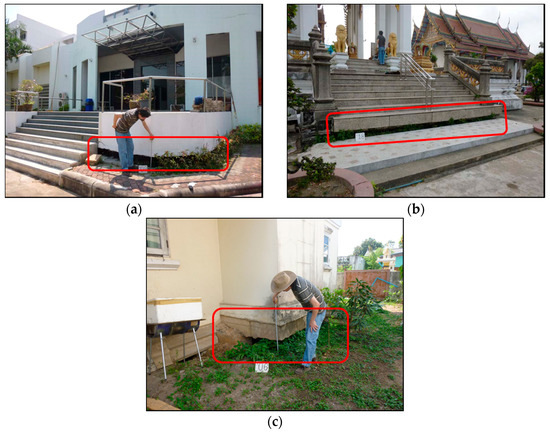
Figure 1.
Differential settlement (DS) of buildings observed in Bangkok, Thailand: (a) a building at King Mongkut’s Institute of Technology Ladkrabang with a gap height of 240 mm; (b) an old temple with a gap height of 492 mm; and (c) a residential house with a gap height of 476 mm. The red rectangles denote the observed DS.
A better understanding of DS in an area of subsidence could be achieved if it were studied over a large area, such as by analyzing multi-temporal satellite images. The interferometric synthetic aperture radar (InSAR) technique can be used to determine ground elevation by taking the phase difference between two synthetic aperture radar (SAR) images and converting it into vertical change. An extension known as the differential InSAR (DInSAR) technique measures subsidence rates by taking the double phase difference, detecting the displacement of objects along the radar line of sight (LOS) and converting it into the vertical displacement. As an extension of DInSAR, the persistent scatterer interferometry (PSI) technique utilizes multi-temporal SAR images and extracts permanent (or persistent) scatterers (PSs) in SAR images that are temporarily-stable natural reflectors. Time-series displacement rates can be estimated from the PSI techniques—such as permanent scatterer InSAR (PSInSAR) [8], small baseline subset (SBAS) [9] and SqueeSAR [10]—even in urban areas [11,12,13,14]. A PSI approach has been extended in terms of the baseline configuration, pixel selection criterion or deformation models [15,16,17]. An extensive review of the PSI is introduced in [18].
Some of the PSs are parts of man-made structures, such as bridges, facades, or buildings. Therefore, it might be possible to determine the subsidence rates of buildings from the rates of PSs. However, we observed in our preliminary study that most of the PSs are detected either at the ground around a building or on the building itself. This fact indicates that rates estimated from such PSs are associated partly with the ground surface and partly with the building. In addition, PSI can generate the information about the PS height from the surrounding surface. Based on this finding with the height information, we aimed to develop a method for distinguishing ground-derived PSs (gPSs) from structure-derived PSs (sPSs), thereby allowing the DS between them to be determined. The remainder of this paper is organized as follows: the study area and data used are reported in Section 2. Section 3 describes the new method. After we report experimental results and discuss them in Section 4 and Section 5, respectively, we conclude this paper in Section 6.
2. Study Area and Dataset
We selected Bangkok, Thailand, as the study area in this study because DS is observed in its eastern outskirts. We used 20 TerraSAR-X strip map images observed from September 2009 to December 2011 on a descending orbit [19] (Table 1). The transmitting-receiving polarization of the radar used to acquire the images was horizontal, expressed as HH. The resolution of each SAR image is approximately 3.3 m in the azimuth and 1.2 m in the range direction. We also used the Shuttle Radar Topography Mission 3 (SRTM3) digital elevation model (DEM), with a nominal resolution of 30 × 30 m, to remove phase fringes induced by the topography [20]. These data were generated from InSAR on board the Space Shuttle. Theoretically, the DEM should represent the elevation of the land surface, but, in reality, the SRTM3 data represent the heights of objects on the surface (e.g., the tops of buildings and the canopy layers of forests) because the data were generated from the radar scattering on the object. In this study, we call the SRTM3 data the DSM and refer to the actual land elevation data as the DEM because this difference is important when discriminating sPSs from gPSs.

Table 1.
Observation dates of 20 TerraSAR-X images. No. 14, in italic letters, represents the master image.
To validate the estimated DS rate, we conducted a field survey in which we measured vertical gaps at 73 sites. For the calibration of the estimated rates, we used 15 one meter-deep levelling data points measured by the Royal Thai Survey Department (RTSD) in an annual levelling survey [21]. The measurements are those of the first-order levelling survey, and their accuracy is at the centimeter level. To estimate the building density reported later, we used two Advanced Land Observing Satellite (ALOS)/Phased Array Type L-band SAR (PALSAR) Level 1.1 (L1.1) images acquired on 3 October 2010 on an ascending orbit [22]. The data were acquired in full-polarization mode, namely four different combinations of horizontal (H)- and vertical (V)-polarization reception and transmission: HH, HV, VH and VV.
3. Methods
The proposed method follows conventional PSInSAR processing and, additionally, implements PS classification and the subtraction of estimated displacement rates. Here, we describe the master-image selection, PS selection and PS classification to understand how the proposed method differs from conventional PSInSAR methods. The DS rate is estimated by taking the difference between the sPS and the gPS nearest to the sPS.
Note that PSI analysis usually uses elevation data (i.e., DEM). However, the data used in most of the analysis represent the surface height, not the elevation, e.g., the SRTM DEM described in the previous section. Because this difference is important for this research, we refer to them as the digital surface models (DSMs). In estimating the displacement rate by minimizing an objective function, the DSM error is also estimated. This is defined as the error between the estimated DSM and the actual DSM.
3.1. Master-Image Selection
Estimation of the displacement rate (vx) and the DSM error (hx) at pixel x uses the coherence given by:
Here, N is the number of interferograms, is the perpendicular baseline [23], is the signal wavelength, is the DSM error height, is the slant distance between sensor and target and is the incident angle. βv and βh are coefficients. In general, the master image is selected from the SAR images by maximizing the stack coherence, expressed as [24]:
Here, T is the temporal baseline and a1 and a2 are constants.
3.2. PS Selection
In the first round of processing, we basically followed the general concepts and outlines of the conventional methods introduced by Ferretti et al. [8] for PSInSAR. For the PS candidate (PSC) selection, we conducted not only amplitude analysis, but also phase analysis [25]. In the amplitude analysis step, we calculated the amplitude dispersion index [8], expressed as:
This process reduces the initial number of pixels for the next step, namely phase analysis.
First of all, we calculate the differential interferogram phase. After removing the topographic phase using the external DSM, the phase () of the x-th pixel in the i-th unwrapped differential interferometric phase is expressed as
where is the phase due to the inaccuracy of the external DSM, is the phase due to the displacement of the PS, is the phase due to atmospheric delay, is the phase due to orbital error and is the decorrelation noise.
In Equation (7), the contribution of the first four terms on the right-hand side dominates the noise term, making it difficult to identify those pixels whose phases have a low standard deviation. Therefore, to obtain an estimate for the noise term (), these four terms should be estimated and removed from the interferometric phase . The first four terms on the right-hand side of Equation (7) are spatially correlated, except for the DSM error , which tends to be only partly spatially correlated. To estimate the spatially-correlated component of the phase, Hooper and Zebker [25] proposed applying a bandpass filter that adapts to any phase gradient present in the data. They implemented a bandpass filter as an adaptive phase filter combined with a low-pass filter, applied in the frequency domain.
First, each pixel is weighted by setting the amplitude in all interferograms to an estimate of the signal-to-noise ratio (SNR) for the pixel; in the first iteration, this is set as . The complex phase of the weighted pixels is sampled to a grid with a spacing of a designated threshold that will enable a two-dimensional (2D) fast Fourier transform (FFT) to be used. The 2D FFT is applied to a grid, and the intensity is smoothed by convolution with a Gaussian window, as shown in Equation (8). The adaptive phase filter response is combined with a narrow low-pass filter response to form the new filter response expressed by Equation (9). By applying the new filter to the resampled observed phase in the frequency domain, namely , the spatially-correlated phase component () will be obtained after applying the 2D inverse FFT given by Equation (10):
where is the fifth-order Butterworth filter with a typical cut-off wavelength of 800 m and is the median value of .
Next, we subtract the filtered phase () from the observed phase () and conduct rewrapping. This will give an estimation of the spatially-uncorrelated phase, namely:
where the superscript u denotes the unwrapped phase. The second term on the right-hand side of Equation (11) is expected to be small; therefore, we replace this term by . As for the first term, the effect of the DSM error () can be estimated using a periodogram:
Subtracting the estimated phase due to the DSM error, , from Equation (12) and assuming , we derive Equation (13) as the first estimation of the noise component ():
When using the estimated noise phase or to calculate the SNR for every pixel we use Equation (12), where is the signal amplitude that is assumed to be constant, is the observed amplitude and is the noise variance. Finally, to get a better estimate for the noise phase, the process should be repeated using the estimated SNR as a weight factor. The system converges when the difference of between iterations ceases to decrease. In this analysis, we chose selected PSCs (SPSCs) by setting a threshold value based on a designated threshold for the final estimation of .
Next, we address the removal of the orbital error. In the general PSI processing, the orbital error term () and atmospheric delay term () are treated together because both effects are similar between neighboring pixels and can be regarded as the residual phase when we consider the difference () between neighboring SPSC pixels along all the arcs of the SPSC network. The SPSC network is generated by applying Delaunay triangulation to SPSCs. We applied orbital-phase error correction to the wrapped interferograms to avoid phase-unwrapping error. The orbital-phase error term is assumed as a linear plane. The linear phase ramp parameters and of the i-th interferogram, without phase unwrapping, are estimated via a simple periodogram expressed as:
where M is the number of SPSC pixels; and are the range and azimuth coordinates, respectively, at the points; and is an indicator of how well the linear plane model fits to the interferogram. After orbital error removal, we estimated the parameters on the arcs using refined interferograms and integrated the estimated parameters along the arcs, generating the linear displacement rate and DSM error height at the remaining SPSC pixels, which we finally regarded as PSs.
Finally, we describe the PS density increment step. In this step, we estimate the parameters on the PSCs points that are rejected as SPSCs in the phase analysis step. Connecting with four neighboring SPSCs, the phase differences are calculated and the parameters on the arcs are estimated on all the connected arcs. This obtains the temporal coherence vector (), the linear displacement rate difference vector () and the DSM error height difference vector (). If the mean of the coherence vector exceeds 0.9, we add the PSC as a PS point and estimate the parameters as:
We calculate this step for all the remaining PSCs. For the filtering step to estimate the nonlinear displacement terms from the residual phase, we used a 2D Gaussian filter in space and a one-dimensional Gaussian filter in the time domain.
3.3. PS Classification
For each PS, the proposed method calculates the value of ‘DSM error + DSM value − DEM value’, which we call the PS height. It is assumed to represent the height of man-made structures from the ground. To classify the PSs, we use the estimates obtained by PSI processing. We generate the DEM by extracting the locally lowest value of the DSM within a certain size of a window. This is known as filtering [26] in the field of three-dimensional point cloud processing.
We generated the probability distribution of the PS height. Assuming that K normal distributions are mixed, the probability density function p(x) and its log-likelihood function are defined by Equations (17) and (18), respectively.
Here, and denote the mean, the variance–covariance matrix and the ratio of the probability density function for class k. These are estimated by applying the expectation-maximization (EM) algorithm [27,28] and decomposing the probability distribution into k normal distributions. The EM algorithm repeats the ‘E’ and ‘M’ steps until the estimates converge. The E step computes the expectation of the log-likelihood function by using tentative estimates, and the M step solves the expectation and updates the estimates.
For the gPSs, the value should be around zero because the DSM value should be equal to the DEM value. However, the mean of the probability density function for the gPSs may not be zero. In reality, each probability distribution composed of the PS height distribution does not follow a normal distribution. However, we recognize that it is acceptable to fit a normal distribution to the PS height distribution because it is important to determine the bias for the PS height and generate the sPSs. An accurate fit is not required. The estimated mean of the probability density function for the gPSs was assumed to be a bias contained in the DSM. After removing this bias, we set a designated threshold to the PS height. We generated sPSs, the PS heights of which were not smaller than the threshold, and gPSs, the PS heights of which were smaller than a designated threshold.
4. Results
4.1. Differential Settlement in Bangkok
In the experiment, we set a1 and a2 in Equation (3) to 3 year (y) and 1300 m, respectively. As a result, the image observed on 19 November 2010 was selected as the master image with respect to which 19 interferograms were generated. The threshold for the amplitude dispersion index in Equation (6) was set to 0.3. The threshold for sampling the complex phase of the weighted pixels was set to 200 m. The 2D FFT was applied to a grid size of 32 × 32 cells, and the intensity was smoothed by convolution with a 7 × 7 pixel Gaussian window in Equation (8). The threshold for selecting SPSCs was set to 0.9. As for the filtering step in the PS density increment step, we used a 200 × 200 m 2D Gaussian filter in space and a 365-day one-dimensional Gaussian filter in the time domain. The thresholds for the 2D FFT, i.e., 32 × 32 cells and 7 × 7 pixel, are from [25]. The other values were determined through experiments with sample data. The processing codes running on MATLAB R2017b [29] were developed by the authors.
Maps of the rates from gPS and sPS of DS over the entire study area are shown in Figure 2b–d, respectively. Figure 2d was generated by subtracting the result of Figure 2b from that of Figure 2c. The rates shown in Figure 2b–d is along the LOS. To save computing time, we divided the study area into six sub-areas that each have one to three points at which a levelling survey has been conducted. For calibration purposes, we calculated the settlement rate of each levelling point from 2009 to 2011 based on available data. We next determined the mean settlement rate from the gPS nearest to each levelling point. We then subtracted the mean settlement rate of the gPSs from that of the levelling point. We finally added the difference to the settlement rate of gPSs and sPSs to realize the absolute settlement rate.
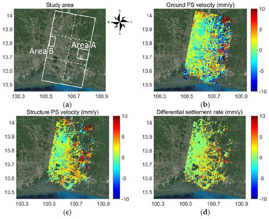
Figure 2.
Differential settlement (DS) rate in Bangkok region from 25 November 2009 to 3 December 2010. (a) Optical image of Bangkok (Google Maps). The larger white parallelogram denotes the area of the satellite images. The smaller parallelograms denote Areas A and B. (b) Ground-derived PS (gPS) rate; (c) structure-derived PS (sPS) rate; (d) DS rate maps. The background images used in the panels were provided by Google [30] and Copernicus.
Figure 3 and Figure 4 show enlarged images of Areas A and B, respectively, as defined in Figure 2a. Area A is the eastern outskirt of Bangkok and includes Suvarnabhumi International Airport. Area B is a moderately-populated area in the city and contains mid-rise and high-rise buildings. Figure 3a and Figure 4a show the respective DSMs. The DEM was generated from the DSM by taking the locally minimum height within a window of 100 × 100 m. The proposed method calculated the PS height, as shown in Figure 3b and Figure 4b. This height was used to distinguish sPSs from gPSs via thresholding. We set the threshold to 5 m to extract sPSs reliably. The classification results are shown in Figure 3c and Figure 4c.
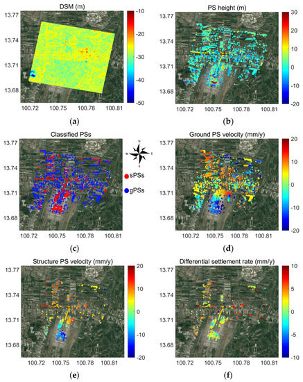
Figure 3.
Enlarged maps for Area A. (a) Digital surface model (DSM); (b) PS height; (c) classified PSs; (d) gPS velocity; (e) sPS velocity; and (f) DS rate. In (c), red and blue points denote sPSs and gPSs, respectively. The background images used in the panels were provided by Google [30] and Copernicus.
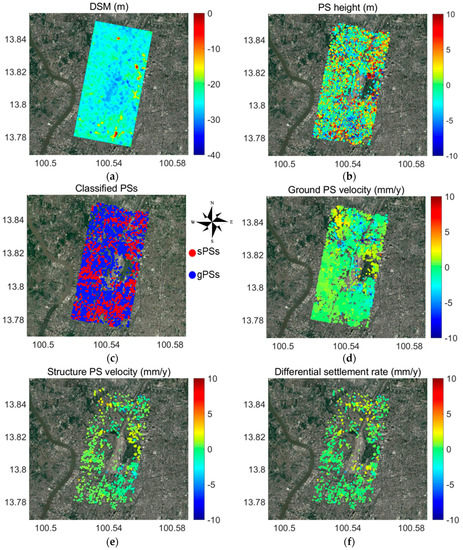
Figure 4.
Enlarged maps for Area B. (a) DSM; (b) PS height; (c) classified PSs; (d) gPS velocity; (e) sPS velocity; and (f) DS rate. In (c), red and blue points denote sPSs and gPSs, respectively. The background images used in the panels were provided by Google [30] and Copernicus.
The estimated settlements of the gPSs are shown in Figure 3d and Figure 4d, while those of the sPSs are shown in Figure 3e and Figure 4e. The DS was finally estimated by subtracting the settlement of the sPS with the average of the settlement of gPSs in a radius of 150 m. Note that, as seen in the points in Figure 3d,e, gPSs and sPSs do not overlap even though they seem to overlap because the points are shown at a larger size. The maps of DS are shown in Figure 3f and Figure 4f. We observed a large DS in Area A, but relatively small, or even negative values (rebound), in Area B. Figure 5 shows the results of decomposing the DSM error probability distributions by assuming that they contain the probability distributions of gPSs and sPSs. As for Area A, the means of the probability distributions of gPS and sPS were −1.1 and 8.6 m, respectively, and the standard deviations were 8.9 and 4.2 m, respectively. As for Area B, the means of the probability distributions of gPS and sPS were 0.8 and 6.3 m, respectively, and the standard deviations were 3.0 and 7.0 m, respectively.
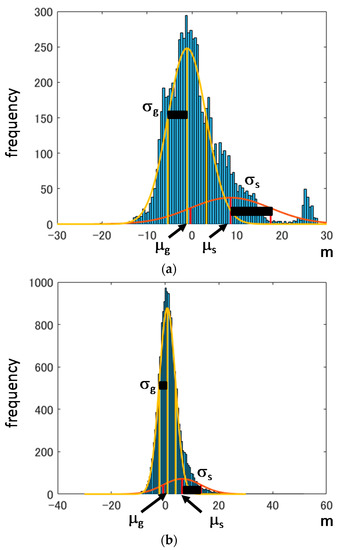
Figure 5.
DSM error probability distributions of gPS and sPS. μg and μs denote the means of the probability distributions of gPS and sPS, respectively. μg and μs denote the standard deviations of the probability distributions of gPS and sPS, respectively. The bin of the horizontal axis was set to 0.5 m. (a) Area A and (b) Area B.
4.2. Validation
We assessed the estimated DSs by comparing them with field measurements. We measured the vertical gaps between the bases of man-made structures and the surrounding ground and compared estimated DSs and field measurements at 71 sites, including 31 in Area A and 18 in Area B. The in situ DS rates were determined by dividing the vertical gaps by the ages of the structures. Where no information was available about the construction date, we simply assumed an age of 20 y by considering the appearance of the buildings available in the study area and estimating the average age. On the other hand, the DS rate was determined along the LOS. To compare the results with the in situ data, the estimated DS values were simply divided by the cosine of the incidence angles at the points, assuming that there was no appreciable horizontal movement in the study area.
As shown in Figure 6, the root-mean-square error (RMSE) of the DS rate was 5.3 mm/y for a sample number of 71. In another case, we assumed a regression model without offset, namely y = β x, where y is the estimated DS rate, x is the actual DS rate and β is a coefficient. The result was β = 0.37847, with an RMSE of 2.35 mm/y and a t-value of 10.474 with a degree of freedom of 70.
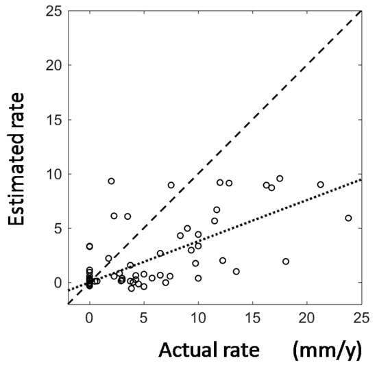
Figure 6.
Comparison between estimated and actual DS rates. The dashed line is where the estimated and actual DS rates are equal, and the dotted line denotes the regression line without offset.
5. Discussion
5.1. Effect of Geological Strata and Building Density
In this section, we discuss the influences of geological formation and building load on DS. It is well known that Bangkok is located on a thick, highly-compressible soft clay layer [5,6]. The subsoil layering is relatively uniform over the entire city area and consists of a 10–15 m-thick layer of soft marine clay that is underlain by a very thick series of alternating stiff to hard clay and sand and gravelly sand [31]. By extracting the thickness of each soil layer from soil boring records at 226 sites across the city [32], the thickness map of each soil layer was generated with the kriging interpolation method by RockWorks [33]. The available geological data show the following ground strata from shallowest to deepest: soft clay, medium stiff clay, stiff clay, first sand and hard clay. The thickness of each layer is shown in Figure 7a–d, and the combined thickness of the three upper clay layers is shown in Figure 7e.
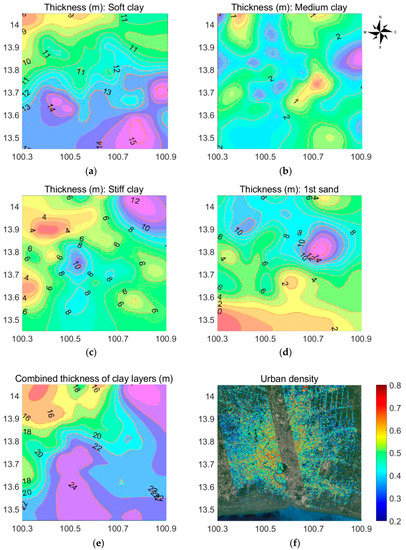
Figure 7.
Geological strata and building density maps. (a–d) show the thicknesses of the soft clay, medium stiff clay, stiff clay and first sand layers, respectively; (e) the combined thickness of the top three clay (soft, medium and stiff) layers and (f) urban density. The background image used in (f) was provided by Google [30] and Copernicus.
It has been reported that land subsidence is ongoing in eastern Bangkok, including Area A, but that no appreciable land subsidence is observed in central Bangkok [34], and Figure 2b supports these assertions. As for the building load, we have previously reported an algorithm for estimating the density of buildings in urban areas from fully-polarimetric SAR images acquired with polarizations of HH, HV, VH and VV [35,36]. Here, ‘H’ denotes horizontal polarization and ‘V’ denotes vertical polarization. A pair of letters denotes the transmitting (first letter) and receiving (second letter) polarizations of the radar used to acquire the images. Our algorithm overcomes the shortcomings of SAR data in that the backscattering from objects is very sensitive to the orientation angle between the radar and the normal of the scattering surface of the object. The method removes the effects of the polarization orientation angle (POA) by rotating the coherency matrix obtained from a fully-polarimetric SAR image and then calculating the mean and standard deviation of the scattering power by the POA domain. It was, thus, demonstrated that the estimated urban density is highly correlated with the building-to-land ratio derived from the geographic information system (GIS) data. Figure 7f shows the density of buildings in the study area. Area A used to be marshland before Suvarnabhumi Airport opened in 2006, and there are still fewer buildings in this area compared to Area B. Area B is a moderately-populated area in the city and contains low- and mid-rise buildings as reflected in the urban density map in Figure 7f.
By comparing Figure 2 and Figure 7f, the settlement of PSs and the DS seems to be uncorrelated with urban density. The building load due to high urban density may induce more ground settlement, but this factor is not comparable to the influence of the excessive use of ground water. This additional settlement due to the building load is unlikely to increase the DS because the sPSs and gPSs settle by the same amount. As mentioned in our Introduction, the tips of piles for high-rise buildings are normally located in the second sand layer, which lies at a depth of 30–58 m from the ground surface [6]. Because the piles are stiffer than the soft clay layer, the ground around a building will settle fasters than the building. This feature is supported by the comparison between Figure 2 and Figure 7f.
By contrast, the settlements of ground (Figure 2b) and buildings (Figure 2c) seem to depend on the combined thickness of the upper clay layers (Figure 7e), as does the DS. Nevertheless, very little DS is observed where the clay layers are thickest. This phenomenon can occur in cases in which the ground and buildings settle at the same rate, for example when a building is supported by short piles.
5.2. Validity of the Proposed Method
The PSI technique has been applied to the detection of building deformation [37,38] where PSs were utilized. Unlike such research, the proposed method can generate three types of displacement maps: ground subsidence, structure subsidence and DS. Users can select and use whichever meets their needs, e.g., to determine the building types in an area of subsidence. Because mid-rise buildings and large structures (e.g., the airport) are built on long piles, a large DS is observed in such areas. By contrast, the north-eastern part of the study area shows relatively large gPS velocity (Figure 2b) and sPS velocity (Figure 2c), but small DS (Figure 2d). These data indicate that the buildings in this area sit on shallow foundations or small piles that settle in the same order as the ground.
Our method outperforms existing methods in two respects, namely (1) classifying PSs into gPSs and sPSs and (2) using the analysis to produce fewer noisy PSs. First of all, we highlight the benefit of the proposed method in relation to estimating accurate rates of land subsidence. The conventional PSI approach does not discriminate between gPSs and sPSs and, therefore, estimates a ground displacement rate that is biased by the building displacement rate. The proposed method improves the accuracy because it discriminates between gPSs and sPSs by referring to the estimated mean of the probability distribution of gPSs (Figure 5). Therefore, it can be used to estimate both the DS rate and the absolute displacement rate of the land. We reason that the proposed method could be applied to various applications for detecting terrestrial displacement.
Next, we discuss the analysis used to have fewer noisy PSs and strengthen the PS network. The conventional PSI approach selects PSCs using a dispersion index [8]. Assuming that multi-temporal complex (amplitude and phase) data are available in a pixel, the dispersion index is defined as a ratio of the standard deviation of amplitude to the mean of amplitude. The lower the dispersion index of a pixel, the more stable the scatterer at that pixel is. If a relatively low threshold is set for the dispersion index (e.g., 0.1 or 0.15), stable pixels are extracted as PSCs. However, the number of PSCs will be limited, and thus, they will be far apart, meaning that local displacement rates cannot be estimated. However, if a relatively high threshold is set (e.g., 0.3 or 0.35), far more PSCs will be generated, but may include unstable scatterers that affect neighboring PSCs. As a result, parts of the PSC network may be rejected because of low stability, meaning that the final map lacks estimation accuracy. Consequently, it is difficult to determine the optimum dispersion-index threshold in the conventional approach.
The proposed method sets a relatively large threshold for the dispersion index (e.g., 0.3) to the relatively small dataset of 20 images and generates many PSCs. It additionally analyzes the phase residual between the estimated phase and the actual phase, which is derived in estimating the displacement rate. SPSCs are chosen among the PSCs according to whether their phase residual is lower than a designated threshold. The proposed method then increases the PS density. In this step, we estimate the parameters on those PSCs that were rejected as SPSCs in the phase-analysis step. By connecting with four neighboring SPSCs, the phase differences are calculated and the parameters on the arcs are estimated on all the connected arcs, leading to the temporal coherence vector (), the linear displacement rate difference vector () and the DSM error height difference vector (). If the mean of the coherence vector exceeds 0.9, we add the PSC as a PS and estimate its parameters. This approach was found to lead to more stable PSs and, thereby, a stable map of the DS rate.
We now discuss why the DS rate is underestimated in comparison to the surveyed value. Based on the theory of consolidation in the field of geotechnical engineering, ground does not settle at a constant rate. The settlement rate is larger in the early stage of settling and then reduces greatly in a logarithmic manner [39]. For example, instrumentation at Kansai International Airport in Osaka in Japan showed that the settlement in the diluvium clay layer was approximately 6 m in the first decade of operation and then reduced to only 2.4 m in the second decade [40,41]. Because only cumulative settlements can be observed in the field, the DS rate that is derived by dividing the cumulative settlement by the building age represents the overall rate of settlement, also known as the secant rate. Meanwhile, the estimated DS rate from SAR images was determined from data acquired between September 2009 and December 2011. Because some consolidation may have already occurred before the analyzed period, it is not uncommon for the estimated values, which are determined tangentially, to be smaller than the surveyed values.
We conclude that the proposed method can automatically and effectively generate three wide-area maps of displacement, namely ground displacement, structure displacement and DS. The proposed method leads to more PSs and classifies them into gPSs and sPSs. As a result, the accuracy of the ground displacement velocity is improved, and as by-products, maps of structure displacement and DS can be generated. These maps have the potential to be used in various fields of science and engineering to understand the DS and land subsidence of megacities.
6. Conclusions
This paper presents the detection of and insight into ongoing DS of man-made structures in Bangkok, Thailand, using the DInSAR technique. DS is defined as a gap between the base of a building and the surrounding ground surface. The proposed method implements PSInSAR and classifies PSs into ground-derived PSs and man-made structure-derived PSs. Subtraction of the displacement rate of gPSs from that of the sPSs can detect the differential settlement rate. In processing, we improved the PS selection so as to increase the number of PSs, which is one of the most challenging issues for stable and accurate DInSAR analysis. Comparison with field survey data revealed that the RMSE of the DS rate was 5.3 mm/y for a sample number of 71, and this has demonstrated the possibility of applying our approach to the detection of areas in which DS is occurring. In the near future, the authors will examine improvements of the proposed method and applicability to the long-term dataset.
Author Contributions
M.T. and N.M. developed the method, and M.T. processed the satellite data. J.S., T.B. and N.M. (mainly J.S. and T.B.) conducted the field surveys. J.S., N.M. and T.B. wrote the manuscript with extensive input from the other author.
Funding
This research was supported by a Japan Society for the Promotion of Science (JSPS) Grant-in-Aid for Scientific Research (KAKENHI) for Challenging Exploratory Research (16K14298), by the European Space Agency (ESA) through providing the TerraSAR-X images and by a program of the Sixth Advanced Land Observing Satellite-2 Research Announcement, Japanese Aerospace Exploration Agency through providing the PALSAR images.
Acknowledgments
This research was supported by a Grant-in-Aid for Scientific Research (KAKENHI) for Challenging Exploratory Research (16K14298), by the European Space Agency (ESA) through providing the TerraSAR-X images and by a programme of the Sixth Advanced Land Observing Satellite-2 Research Announcement, Japan Aerospace Exploration Agency, through providing the PALSAR images.
Conflicts of Interest
The authors declare no conflict of interest.
References
- Erban, L.E.; Gorelick, S.M.; Zebker, H.A. Groundwater extraction, land subsidence, and sea-level rise in the Mekong Delta, Vietnam. Environ. Res. Lett. 2014, 9, 084010. [Google Scholar] [CrossRef]
- Caló, F.; Notti, D.; Galve, J.P.; Abdikan, S.; Görüm, T.; Pepe, A.; Balik Şanli, F. DInSAR-based detection of land subsidence and correlation with groundwater depletion in Konya Plain, Turkey. Remote Sens. 2017, 9, 83. [Google Scholar] [CrossRef]
- Reul, O.; Randolph, M.F. Piled rafts in overconsolidated clay: Comparison of in situ measurements and numerical analyses. Géotechnique 2003, 53, 301–305. [Google Scholar] [CrossRef]
- Arapakou, A.E.; Papadopoulos, V.P. Factors affecting differential settlements of framedstructures. Geotech. Geol. Eng. 2012, 30, 1323–1333. [Google Scholar] [CrossRef]
- Phien-wej, N.; Giao, H.P.; Nutalaya, P. Land subsidence in Bangkok, Thailand. Eng. Geol. 2006, 82, 187–201. [Google Scholar] [CrossRef]
- Boonyatee, T.; Tongjarukae, J.; Uaworakunchai, T.; Ukritchon, B. A review on design of pile foundations in Bangkok. Geotech. Eng. 2015, 46, 76–85. [Google Scholar]
- Anuphao, A. InSAR Time Series Analysis for Land Subsidence Monitoring in Bangkok and Its Vicinity Area. Ph.D. Thesis, Department of Survey Engineering, Chulalongkorn University, Bangkok, Thailand, 2012. [Google Scholar]
- Ferretti, A.; Prati, C.; Rocca, F. Permanent scatterers in SAR interferometry. IEEE Trans. Geosci. Remote Sens. 2001, 39, 8–20. [Google Scholar] [CrossRef]
- Berardino, P.; Fornaro, G.; Lanari, R.; Sansosti, E. A new algorithm for surface deformation monitoring based on small baseline differential SAR interferograms. IEEE Trans. Geosci. Remote Sens. 2002, 40, 2375–2383. [Google Scholar] [CrossRef]
- Ferretti, A.; Fumagalli, A.; Novali, F.; Prati, C.; Rocca, F.; Rucci, A. A new algorithm for processing interferometricdata-stacks: SqueeSAR. IEEE Trans. Geosci. Remote Sens. 2011, 49, 3460–3470. [Google Scholar] [CrossRef]
- Ferretti, A.; Prati, C.; Rocca, F. Non-linear subsidence rate estimation using permanent scatterers in differential SAR Interferometry. IEEE Trans. Geosci. Remote Sens. 2000, 38, 2202–2212. [Google Scholar] [CrossRef]
- Stramondo, S.; Bozzano, F.; Marra, F.; Wegmuller, U.; Cinti, F.R.; Moro, M.; Saroli, M. Subsidence induced by urbanisation in the city of Rome detected by advanced InSAR technique and geotechnical investigations. Remote Sens. Environ. 2008, 112, 3160–3172. [Google Scholar] [CrossRef]
- Perissin, D.; Wang, T. Time-series InSAR applications over urban areas in China. IEEE J. Sel. Top. Appl. Earth Obs. Remote Sens. 2012, 4, 92–100. [Google Scholar] [CrossRef]
- Chaussard, E.; Wdowinski, S.; Cabral-Cano, E.; Amelung, F. Land subsidence in central Mexico detected by ALOS InSAR time-series. Remote Sens. Environ. 2014, 140, 94–106. [Google Scholar] [CrossRef]
- Goel, K.; Adam, N. A distributed scatterer interferometry approach for precision monitoring of known surface deformation phenomena. IEEE Trans. Geosci. Remote Sens. 2014, 52, 5454–5468. [Google Scholar] [CrossRef]
- Lv, X.; Yazici, B.; Zeghal, M.; Bennett, V.; Abdoun, T. Joint-scatterer processing for time-series InSAR. IEEE Trans. Geosci. Remote Sens. 2014, 52, 7205–7221. [Google Scholar]
- Devanthéry, N.; Crosetto, M.; Monserrat, O.; Cuevas-González, M.; Crippa, B. An approach to persistent scatterer interferometry. Remote Sens. 2014, 6, 6662–6679. [Google Scholar] [CrossRef]
- Crosetto, M.; Monserrat, O.; Cuevas-González, M.; Devanthéry, N.; Crippa, B. Persistent scatterer interferometry: A review. ISPRS J. Photogramm. Remote Sens. 2016, 115, 78–89. [Google Scholar] [CrossRef]
- German Aerospace Center (DLR). TerraSAR-X—Germany’s Radar Eye in Space. Available online: http://www.dlr.de/dlr/en/desktopdefault.aspx/tabid-10377/565_read-436/#/gallery/350 (accessed on 2 February 2018).
- U.S. Geological Survey (USGS). Shuttle Radar Topography Mission (SRTM) 1 Arc-Second Global. Available online: https://lta.cr.usgs.gov/SRTM1Arc (accessed on 2 February 2018).
- The Royal Thai Survey Department. International union of geodesy and geophysics—Thailand reported on the geodetic work period 1999–2002. In Proceedings of the the XXIII General Assembly of the International Union of Geodesy and Geophysics, Sapporo, Japan, 30 June–11 July 2003. [Google Scholar]
- Earth Observation Research Cente (EORC). Japan Aerospace Exploration Agency (JAXA), About ALOS—PALSAR. Available online: http://www.eorc.jaxa.jp/ALOS/en/about/palsar.htm (accessed on 2 February 2018).
- Colesanti, C.; Ferretti, A.; Locatelli, R.; Savio, G. Multi-platform permanent scatterers analysis: First result. In Proceedings of the Second GRSS/ISPRS Joint Workshop on Data Fusion and Remote Sensing over Urban Areas, Berlin, Germany, 22–23 May 2013; pp. 52–56. [Google Scholar]
- Kampes, B.M. Radar Interferometry; Springer: Berlin/Heidelberg, Germany, 2006. [Google Scholar]
- Hooper, A.; Zebker, H. Persistent scatterer interferometric synthetic aperture radar for crustal deformation analysis, with application to Volcán Alcedo, Galápagos. J. Geophys. Res. 2007, 112, B07407. [Google Scholar] [CrossRef]
- Susaki, J. Adaptive slope filtering of airborne LiDAR data in urban areas for digital terrain model (DTM) Generation. Remote Sens. 2012, 4, 1804–1819. [Google Scholar] [CrossRef]
- Dempster, A.P.; Laird, N.M.; Rubin, D.B. Maximum-likelihood from incomplete data via the EM algorithm. J. R. Stat. Soc. Ser. B. 1977, 39, 1–38. [Google Scholar]
- Redner, R.; Walker, H. Mixture densities, maximum likelihood and the EM algorithm. SIAM Rev. 1984, 26, 195–239. [Google Scholar] [CrossRef]
- MATLAB. MathWorks. Available online: https://www.mathworks.com/products/matlab.html (accessed on 5 May 2018).
- Google Earth, Google. Available online: https://www.google.com/earth/ (accessed on 5 May 2018).
- Amornfa, K.; Phienwej, N.; Kitpayuck, P. Current practice on foundation design of high-rise building in Bangkok, Thailand. Lowl. Technol. Int. 2012, 14, 70–83. [Google Scholar]
- Ngamcharoen, K.; Likitlersuang, S.; Boonyatee, T. Development of 3D geological modelling for Bangkok subsoils. In Proceedings of the Twenty-Ninth KKHTCNN Symposium on Civil Engineering, Hong Kong, China, 3–5 December 2016. [Google Scholar]
- RockWorks. RockWare. Available online: https://www.rockware.com/product/rockworks/ (accessed on 5 May 2018).
- Gambolati, G.; Teatini, P. Geomechanics of subsurface water withdrawal and injection. Water Resour. Res. 2015, 51, 3922–3955. [Google Scholar] [CrossRef]
- Kajimoto, K.; Susaki, J. Urban density estimation from polarimetric SAR images based on a POA correction method. IEEE J. Sel. Top. Appl. Earth Obs. Remote Sens. 2013, 6, 1418–1429. [Google Scholar] [CrossRef]
- Susaki, J.; Kajimoto, M.; Kishimoto, M. Urban density mapping of global megacities from polarimetric SAR images. Remote Sens. Environ. 2014, 155, 334–348. [Google Scholar] [CrossRef]
- Bru, G.; Herrera, G.; Tomás, R.; Duro, J.; De la Vega, R.; Mulas, J. Control of deformation of buildings affected by subsidence using persistent scatterer interferometry. Struct. Infrastruct. Eng. 2013, 9, 188–200. [Google Scholar] [CrossRef]
- Bianchini, S.; Pratesi, F.; Nolesini, T.; Casagli, N. Building deformation assessment by means of persistent scatterer interferometry analysis on a landslide-affected area: The Volterra (Italy) case study. Remote Sens. 2015, 7, 4678–4701. [Google Scholar] [CrossRef]
- Terzaghi, K. Theoretical Soil Mechanics; John Wiley and Sons: New York, NY, USA, 1944. [Google Scholar]
- Land Subsidence Status of Kansai International Airport for the Island 1. Available online: http:// www.kansai-airports.co.jp/efforts/our-tech/kix/sink/sink3/sink3_c.html (accessed on 18 February 2018). (In Japanese).
- Land Subsidence Status of Kansai International Airport for the Island 2. Available online: http:// www.kansai-airports.co.jp/efforts/our-tech/kix/sink/sink3/sink3_e.html (accessed on 18 February 2018). (In Japanese).


© 2018 by the authors. Licensee MDPI, Basel, Switzerland. This article is an open access article distributed under the terms and conditions of the Creative Commons Attribution (CC BY) license (http://creativecommons.org/licenses/by/4.0/).