Article

Localization and Extraction of Road Poles in Urban Areas from Mobile Laser Scanning Data

1
Research Institute for Smart Cities & Guangdong Key Laboratory of Urban Informatics & Shenzhen Key Laboratory of Spatial Smart Sensing and Services, School of Architecture and Urban Planning, Shenzhen University, Shenzhen 518060, China
2
Key Laboratory of Urban Land Resources Monitoring and Simulation, Ministry of Land and Resources, Shenzhen 518040, China
3
School of Resource and Environmental Sciences, Wuhan University, Wuhan 430079, China
4
Shenzhen Urban Public Safety and Technology Institute, Shenzhen 518048, China
*
Author to whom correspondence should be addressed.
Remote Sens. 2019, 11(4), 401; https://doi.org/10.3390/rs11040401
Submission received: 23 December 2018 / Revised: 4 February 2019 / Accepted: 12 February 2019 / Published: 16 February 2019
(This article belongs to the Section Urban Remote Sensing)

Abstract

:
Lampposts, traffic lights, traffic signs, utility poles and so forth are important road furniture in urban areas. The fast and accurate localization and extraction of this type of furniture is urgent for the construction and updating of infrastructure databases in cities. This paper proposes a pipeline for mobile laser scanning data processing to locate and extract road poles. The proposed method is based on the vertical continuity with isolation feature of the pole part and the overall roughness feature of the attachment part of road poles. The isolation feature of the pole part is analysed by constructing two concentric cylinders from bottom to top and there should be no or a limited number of, points between these two cylinders. After splitting up the pole part and the attachment part of a road pole, the roughness of the candidate attachment points is computed and the attachment is obtained by performing region growing method based on roughness values. By applying the proposed pipeline to different situations in two datasets, the proposed method proves to be efficient not only in simple scenes but also in cluttered scenes.

Graphical Abstract

1. Introduction

Urban scene interpretation plays an important role in many research areas, such as urban planning [1], road safety management [2], road inventory construction [3], automatic driving and navigation for pedestrians and cars [4,5]. However, traditional methods of urban scene interpretation have always been a problem in the development of geographic information science. Currently, there are two broadly used methods of geographic data acquisition: the manual method and the method that utilizes remote sensing imagery. Both of these methods have limitations. The first method is time-consuming, which leads to the slow updating of geographic information. The second method uses high-resolution satellite imagery, which performs well in the detection and classification of roads, vegetation and buildings of urban scenes but it is rather difficult to use when recognizing relatively small street furniture, such as road poles and the vertical information of buildings is often difficult to acquire.
In the past few years, there has been rapid growth in the use of mobile mapping systems for urban scene interpretation [1,2,6,7,8,9,10,11,12,13]. Most mobile mapping system configurations integrate digital cameras, laser scanners, GPS receivers and antennas, an inertial navigation system (INS) for acceleration and orientation measurements of moving platforms and a wheel-mounted distance measuring indicator (DMI), which provides accurate vehicle velocity updates. The data acquired by laser scanners in mobile mapping systems, usually called mobile laser scanning data, contain detailed information of urban scenes and can be used for the automatic detection of road poles [14,15,16,17,18,19].
Road poles can be defined as street furniture objects along the street in urban scenes that are entirely shaped like poles or those that contain a pole part. For example, lampposts, utility poles and traffic lights are pole-like objects and traffic signs and trees are objects that contain a pole. They are crucial street objects in urban environments because they are very common and distinguishing in urban environments [4]. They can pose a great impact on city planning and management and they are often one of the major subjects in road safety studies [2]. Moreover, the extraction of road poles can be useful in driver assistance systems by providing urban maps [4,5].
The objective of this paper is to present a novel location-based algorithm to automatically recognize road poles in mobile laser scanning data. Section 2 provides an overview of the related work of the proposed method. Section 3 describes the three-stage automatic detection algorithm in sequence. Parameter settings and experimental results are analysed in Section 4. In Section 5, we conclude the proposed method and future work of this research is discussed.

2. Related Works

2.1. Studies on the Recognition of Pole Structures in Point Clouds

Some researchers detect road poles from point cloud data by analysing local geometry features of points in point clouds. Yokoyama et al. assumed that the ground points were removed from the mobile point clouds [14]. The algorithm first segments the point clouds into groups using a k-nearest neighbour graph. To effectively calculate the dimensionality of each point and distinguish the linear points, the second step performs the endpoint preserving Laplacian smoothing. Points are then classified as linear, planar and rough based on neighbouring points using PCA with a fixed radius. A likelihood function was used to determine the degree of the likelihood of a segment being a road pole. Road poles were considered to contain a large portion of linear points in the segments and have many points with principle directions that were vertical to the horizontal plane. In this method, by using smoothing and PCA, robust detection of the road pole with various radii and tilt angles could be obtained. However, the removal of ground points is not trivial and the segmentation results of this method were unsatisfactory. Yang et al. introduced an algorithm to segment 3D street objects from MLS data and performed some experiments with automatic detection of road poles [15]. This method used a new approach to optimistically select the radius of the neighbourhood and used a supervised method to classify the points into linear, planar and spherical points based on a series of local geometry features. These points were segmented into different groups based on the dimensionality of each point and segments were subsequently refined and merged. The segments were recognized as road poles when they had a linear patch that at least touched the ground surface; this linear feature may be attached to planar or spherical patches of certain sizes. Yang et al. further improved their method based on supervoxel analysis, which also incorporated geometric features including normal, principal direction and dimensionality [16]. Both approaches could detect road poles that were far away from the trajectory and that were standing close to each other. However, additional features, such as colours and contextual features, were still needed to improve the detection accuracy of the segmentation and detection of road poles. Li et al. proposed an interesting framework to decompose road furniture into different components based on their spatial relations [20,21,22]. The poles are categorized to three classes and each class of pole is extracted using three different methods. In their research, only geometric features were used to extract road furniture and extracted items have been decomposed into components which will contribute to further classification.
Another effective and popular approach to detect road poles is the model-driven method. The first kind of model-driven method is called the two-cylinder model, which assumes that the pole part of the road poles is upright and there is a kernel region where laser scan points are present and an outside region where no points are present. Berner et al. first introduced this two double cylinder method to detect poles and used the position of the road poles for positioning future driving assistance systems [4]. C. Cabo et al. also applied a similar method to their algorithm. Instead of performing two cylinder analyses directly on the point cloud segment, this method performed a two-circle analysis on the horizontal slices of the point cloud data after voxelization [23]. Shi Pu et al. developed a rectangle model to fit the horizontal slices of points [2]. The segmented candidates were first divided into height percentiles. A certain percentile was chosen and the percentile was further divided into horizontal subparts. By iterating all slices in the percentile, the deviations between neighbouring slices according to the position of the centre point and the length of the diagonal are checked to recognize road poles. Because this method could choose the higher percentile to perform recognition, even road poles standing in bushes could be detected. However, this method utilized connected component analysis to segment the point cloud, which implied that they could not separate road poles that were standing close together. El-Halawanya et al. developed another line model-based method to detect road poles [24]. The advantage of this approach is that no assumptions about the position of the poles are made and poles attached to other objects, such as traffic signs, can be detected as separated objects. The major problem with this method was that the 2-dimensional density-based ground removal method was sensitive to point densities; therefore, road poles that were far away from the trajectory were removed in this stage.
Some other algorithms detect road poles using machine learning and training data. Golovinskiy et al. developed a system to classify different objects, including road poles, in urban scenes from integrated point clouds from the ALS system and MLS system [25]. The whole pipeline consisted of four major parts, localization, segmentation, feature extraction and classification. Several methods were tested in each step and the system was able to recognize approximately 65% of the small objects in the urban environment in the experiments. They used part of the experimental dataset as training data, which were labelled as different classes manually. Lai, K et al. and Ishikawa et al. also developed algorithms to classify urban scenes (including road poles) using machine learning [26,27] The problem with this kind of method is that the manual work of labelling points is laborious and the training data from one dataset may not fit the model of other datasets.

2.2. Studies on Segmentation of Urban Point Cloud into Objects

In simple situations where there is separable space between different objects, the connected component analysis method or the Euclidean distance-based clustering method, which only need a fixed radius configuration, are capable of segmenting point clouds to distinct 3D patches. The literature [2] utilized this method to recognize basic structures from mobile laser scanning data for road inventory studies. After removing the off-ground and ground points, the remaining on-ground points were segmented and assigned with unique IDs by performing connected component analysis using the Euclidian cue. Lehtomäki et al. also applied the connected component analysis algorithm to obtain street object segments after ground and building facades removal [6]. Wang et al. introduced a 3D significant eigenvector based shape descriptor using voxels (SigVox), for the first time, to detect street objects [28]. They also applied connected component analysis based on voxel connectivity to segment individual street furniture for further recognition. Similarly, in Reference [29], the method also configured a fixed radius parameter to distinguish objects with the connected components analysis method. However, this method could recognize more objects in complicated scenes because it introduced a new technique to resegment mixed trees. Because the space between different street objects could vary greatly for objects of different sizes, the method [30] added an extra connected component analysis step after the original connected component analysis algorithm. In the extra step, a large radius was configured for those large segments to overcome oversegmentation and a small radius for those small segments to reduce undersegmentation. The results of their experiments showed that their improved method was better than the connected component analysis method with a fixed radius configuration.
In other situations where objects may connect to each other, the Euclidian distance-based clustering method is not sufficient to segment them out. Due to the presence of noisy data and the variety of object sizes and shapes, a segmentation method using one single cue is not sufficient. To segment out connecting objects more accurately, other cues are needed besides Euclidian distance. The most frequently used cues for discriminating connecting street objects are local neighbourhood-based geometric features, including normal vector, smoothness, roughness, major direction and dimensionality. The methods [16,31] utilized the supervoxel method to highlight the object borders or the object. The supervoxel method only turns neighbouring points with similar colour and intensity values into patches. These oversegmented patches are then merged into objects based on other cues and methods. The graph-cut method [15,16,31,32,33] is a widely used method for segmenting overlapping objects because it can measure the connecting strength between points. The method [15,16] incorporated the geometric features of points, including normal and main directions, to the energy measurement of the normalized cut and used them as a measure between different patches to merge them. In addition, other methods [34] utilized a density-based clustering algorithm to consider the shape distribution of connecting trees and poles to segment them out.
All in all, current methods for street furniture segmentation perform well in many situations. However, these methods need further improvement in complex scenes in two ways which are also the innovations of this paper. First, a new algorithm for street objects localization is needed for point clouds with large density variations. Therefore, we introduced a new 3D density-based street object localization algorithm to detect object locations in such point clouds. Second, we need to find a new method to segment road poles from trees in clutter scenes where trees and road poles are connected or tangled with each other. Thus, a roughness-based analysis for point cloud clusters of tangled street objects was proposed to detect such road poles.

3. Methods

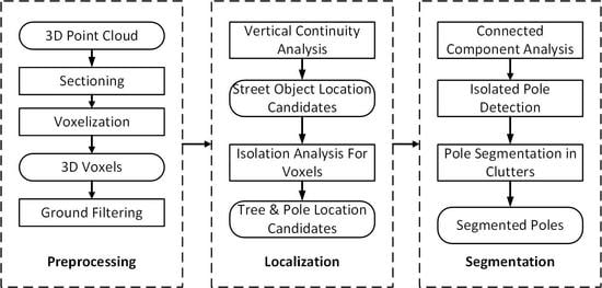
The proposed method aims to segment MLS data of urban scenes into discernible and meaningful segments that represent road poles. The method consists of three main phases (Figure 1):
(1)
Pre-processing: Original unorganized MLS data are sectioned and reorganized based on voxels; then, the whole scene is classified as ground and non-ground voxels.
(2)
Localization: A voxel-based method utilizing isolation analysis to detect the position of poles, including trees.
(3)
Segmentation: Differentiate poles from trees using roughness analysis from isolated segments and segment poles from connected furniture segments by detecting man-made structures.

3.1. Pre-Processing of Original MLS Data

This phase aims to provide clean and organized data for the following localization and segmentation algorithm, including sectioning of the original point cloud, the voxelization of points into voxels and the detection of ground voxels. Due to the complexity of the scanning environment in urban scenes, noise points that are isolated from the rest of the point cloud are brought into the original MLS data. These noise points have a negative effect on the following algorithm; thus, they need to be detected and removed from the original MLS data. Isolated points are detected and removed using the connected component analysis method; small clusters are considered as noisy points and filtered out from the original MLS data. We perform a two-round connected component analysis algorithm to filter out noisy points. In the first round, we connected point within 30 centimetres and filter out clusters with less than 20 points while in the second round we connected points within 50 centimetres and filtered out the clusters with less than 50 points.

3.1.1. Sectioning of Original Data

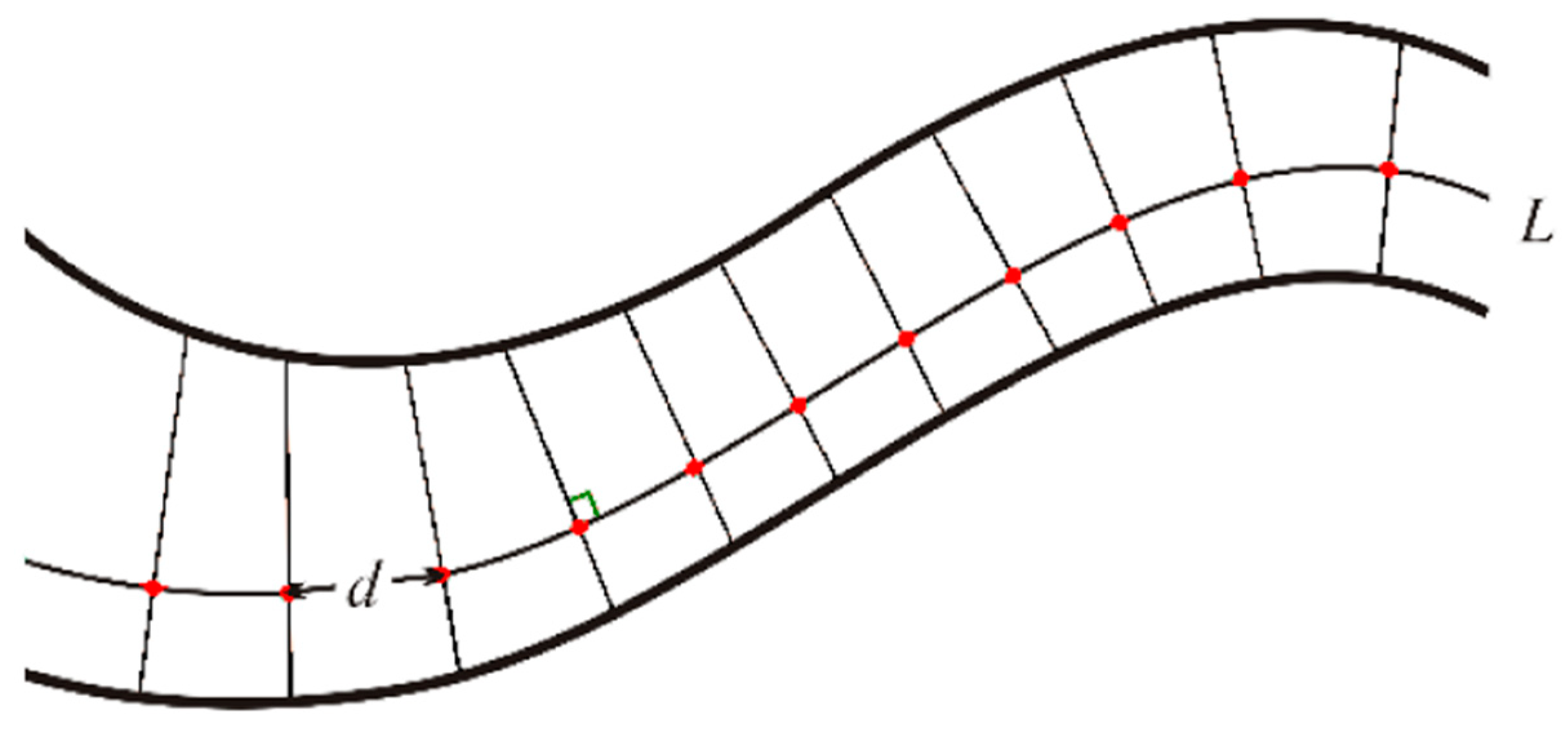
As the original point cloud datasets are usually extremely large, it is wise to first partition the whole data into multiple parts and then to extract the information of interest locally [2]. Huge data volumes and the complexity of urban street scenes make it difficult to create a unified ground model. Therefore, we use the vehicle trajectory data (L) to section the point clouds into a set of blocks at an interval (d), as shown in Figure 2. To ensure that the road in each block is as flat and straight as possible, the value of d should be set smaller in undulating and winding road conditions. The width of our blocks are 100 m and 120 m for the two corresponding test areas. The overlapping zone is 5m in case that road pole candidates are segmented to two parts.

3.1.2. Voxelization

Direct operations on the point cloud will be time- and memory-consuming as original point clouds are both large in volume and unorganized in structure. Thus, after filtering out isolated noise points and sectioning of the original point cloud, we implement a voxelization method similar to (Cabo et al., 2014), which regularly re-organizes and condenses the original data into a new 3D space. In this paper, a voxel is defined as a cube that records three classes of information: voxel location, voxel index and the number of points in the voxel. A voxel location is represented by three numbers ( n r , n c , n h ) , which represents the location of the voxel relative to the minimum x, y and z position of the original point cloud. The location of the voxel can be computed using the following equation:
n r = i n t e g e r ( x x m i n V S )
where x m i n represents the minimum x of all points in the point cloud and V S is the voxel size. n c and n h are calculated in a similar way.
After the processing step of voxelization, all needed information for the steps before the merging processing step is stored in the voxels and the correspondence between voxels and points is constructed.

3.1.3. Ground Detection

The point cloud data in urban scene can be roughly classified as off-ground points, on-ground points and ground points [2]. The segmentation targets in this paper are the road poles that stand on or close to the ground. The ground voxels can be first detected to obtain the target objects. Many previous researchers have attempted to detect or even reconstruct roads in point cloud data [3,35,36,37,38,39,40,41,42]. Roads can sometimes act as the ground to gain the relative position of street furniture to the ground in situations where the ground is mainly vertically even along the trajectory. Nevertheless, in this context, complex situations of wide and uneven streets are taken into consideration. Therefore, we introduced a new ground detection method that operates on a voxel set generated in the previous step.
The ground is assumed to be relatively low in a local area and erected low compared to on-ground objects in the vertical direction. Therefore, the ground can be detected from the whole scene by analysing the relative height ( H r e l a t i v e ) and the vertically continuous height ( H v e r t i c a l ) of each horizontally lowest voxel (HLV) in the whole voxel set. The relative height ( H r e l a t i v e ) parameter describes the relative height between an HLV and the lowest voxel in a neighbourhood. The height of the HLV is represented by n H L V while n a r g m i n ( N ( H L V ) ) depicts the height of the lowest voxel in a neighbourhood of the HLV.
H r e l a t i v e = n H L V n a r g m i n ( N ( H L V ) )
Voxels that satisfy the conditions in Equation (3) are recognized as ground voxels:
H v e r t i c a l < i n t e g e r ( 1 V S )   & &   H r e l a t i v e < i n t e g e r ( 0.5 V S )
H v e r t i c a l is the vertically continuous height of an HLV, which depicts the vertical height of an HLV. The algorithm for calculating H v is depicted in detail in a previous research [3]. Utilizing the proposed algorithm, curbs and low-elevation bushes are also classified as ground and are thus filtered out before segmentation.

3.2. Localization of Poles and Trees

Localization is first carried out to differentiate trees and poles from other objects, including buildings, vehicles, fences and so forth. The localization algorithm consists of two consecutive steps: (1) coarse localization of street objects and (2) selection of trees and poles.

3.2.1. Localization of Street Objects

A typical method for locating street objects is by projecting all 3D points into the horizontal plane and performing 2D density analysis [31,43]. The pixels with large density values in the projected 2D image are assumed to indicate the presence of a street object. However, in our scenes, large density variations exist for different objects and a single density threshold value cannot locate all of the road poles. Therefore, we apply a similar localization method of previous work [34], which implements a 3D density analysis algorithm to locate street objects. The density parameter together with minimum distance parameter are computed to locate the clustering centre for a clustering algorithm in [34], while in the proposed method the density parameter is used only to detect high density voxel. The formula was simplified from the one in Reference [34] for computing efficiency.
Based on the analysis of hundreds of street objects in different scenes, we can reasonably assume that the street objects we are interested in are those that are sufficiently high in the vertical direction. In this 3D density-based street object localization algorithm, we assume that a position with a large density value is the position of a street object. To accurately represent the vertical height of an object, we introduce a new approach to calculate the 3D density values ρ i . For every voxel v i , the density parameter ρ i can be formulated as:
ρ i = { H v i ,            d g r o u n d i < D t H v i / d g r o u n d i ,   d g r o u n d i D t
where d g r o u n d i depicts voxel v i ’s vertical distance to the ground. D t is a ground distance threshold value based on the overall height of lowest tree leaves to eliminate most tree leaves from location candidates [34]. In our experiment, this value was set to 1.2 m as almost all tree leaves are higher than 1.2 m in our datasets. The voxel v i is classified as an object location if its 3D density value ρ i is over a specific threshold value μ (Equation (5)).
{ ρ i < μ ,                         v i   i s   n o t   o b j e c t   l o c a t i o n ρ i μ ,                               v i   i s   o b j e c t   l o c a t i o n
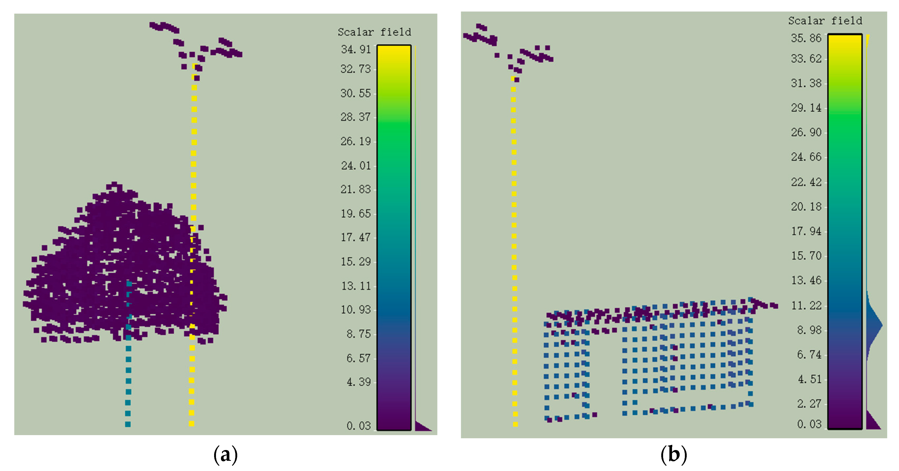
An example for computing the density values for each voxel with the proposed method is depicted in Figure 3. The histogram in each figure depicts the density distributions of all the voxels in the corresponding figure. In the figure, the pole part of a tree and the two poles show high density values and thus can be selected as object locations.
After the coarse classification is implemented, the overall voxels are categorized as object locations and others. As these object location voxels are selected, a connected component analysis process is applied to group these voxels. We allocate the voxel with the largest value and at the bottom of a horizontal location as the location voxel of an object.

3.2.2. Selecting Candidate Locations of Road Poles and Trees

There are two assumptions about the pole part of trees and poles: (1) the diameter of the pole part is at a specified range and (2) there are long enough parts of the pole that are isolated from other objects. Based on these assumptions, we can implement a new isolation analysis algorithm with a double-cylinder model similar to [5,23]. Our algorithm incorporates methods in Reference [5] and [23], the 2-dimensional isolation analysis method for voxels in Reference [23] is improved to 3-dimensional similar to the isolation analysis method for points in Reference [5]. The position of a pole or tree is configured as the centre of the cylinder. The detailed algorithm is depicted as Algorithm 1.
Algorithm 1 Isolation analysis for voxels
Input:
v : one candidate object position
S: a cluster v in
Parameters:
L: height of the cylinder
N: allowed number of noise points in the ring between cylinders
n: layer counter
Ir: radius of the inner cylinder
Or: radius of the outer cylinder
Start:
repeat
(1) Select voxels V from layer n to layer n + L − 1 from S
(2) Build a concentric cylinder with Ir as the inner cylinder radius and Or as the outer cylinder radius, selecting v as the centre, cylinder height starts from n and end at n + L − 1
(3) Count number of points np and number of voxels nv between two cylinders np
(4)  if np < NP && nv < NV
(5)   v is recognized as pole or tree position
(6)   break
(7)  else
(8)    n = n + 1
until all layers of S are reached
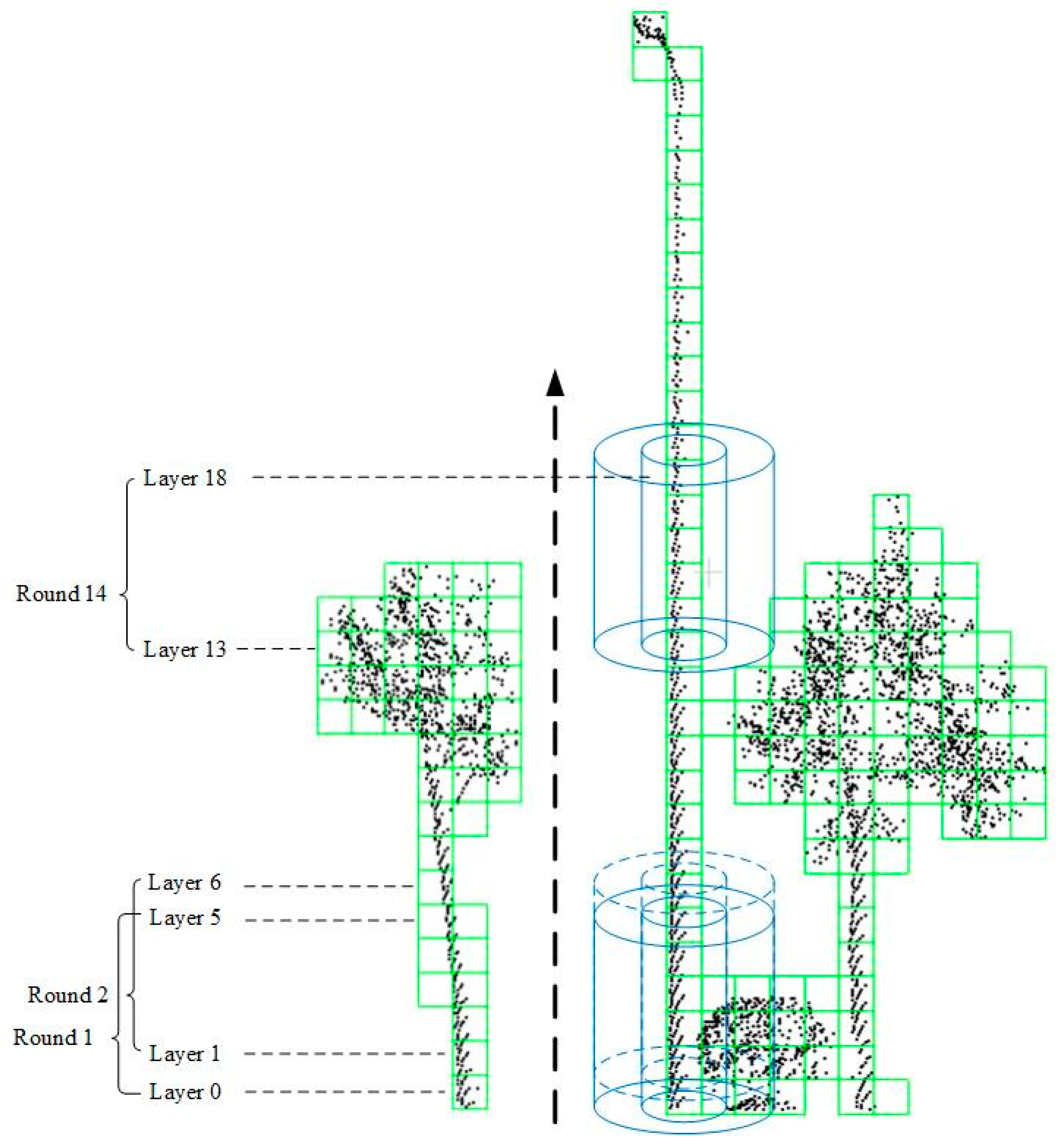
In Figure 4, we present an example of selecting candidate poles and trees with the proposed isolation analysis for voxels algorithm. For the middle lamppost, we perform isolation analysis from the bottom to top. The cylinder parameters are configured based on the radius and height of poles in real situations. Assuming that the cylinder height L is 6, the first two cylinders start from Layer 0 and end in Layer 5 in first round isolation analysis. With one small object standing next to the pole, several points are located between the two cylinders. Thus, the isolation analysis moves upwardly to round 2 and continues from Layer 1 to Layer 6, where there are also points between the two cylinders. The isolation analysis will need to move upwardly again. This cycle ends at round 14 when the bottom of the cylinders reaches Layer 13, where there is no points in between the two cylinders from layer 13 to 18. To this end, this location is selected as a target candidate.
After performing isolation analysis, trees and poles are localized with a localization voxel. Some poles and trees are isolated and a connected component analysis procedure is sufficient to segment them from the environment, while others need further segmentation. The distance of the connected component analysis should be larger than the voxel size. There are three types of clusters after connected component analysis: (1) clusters with no candidate pole position, (2) clusters with one candidate pole position and (3) clusters with more than one candidate pole position. The first kind of cluster is discarded in this step, the second kind of cluster is classified as isolated poles or trees that require further classification and the third kind of cluster is regarded as clusters with multiple trees or poles that require further segmentation.

3.3. Extraction of Road Poles

3.3.1. Detection of Isolated Poles

Trees have crowns with irregular structures, while poles often have regular shapes. Thus, these poles and trees can be classified based on the roughness of their upper part. The roughness of a voxel is determined by the average roughness values of the points inside the voxel. Roughness is a parameter that indicates the random distribution of points. The roughness of a point can be calculated by Equation (6).
r = e 3 e 1
where e 3 is the smallest eigenvalue and e 1 is the largest eigenvalue calculated using principal component analysis. Here, eigenvalues [ e 1 , e 2 , e 3 ] are estimated by constructing a covariance matrix M (Equation (7)) that is generated from a set of neighbouring points N i in a sphere within radius r i of p i .
M = 1 n i = 1 n ( p i p ¯ ) · ( p i p ¯ ) T
where n is the number of points within radius r i of p i and p ¯ is the geometric centroid of the points of N i . To overcome the density variation problem, we utilize an optimal radius algorithm to calculate the r h i parameter [44].
The shape of the upper part of the cluster is classified by averaging the roughness value (calculated using Equation (6)) of the upper part points (Equation (8)).
r h = 1 n i = 1 n r i
where n is the number of points in the upper part of a cluster. Some road poles such as some street lamps, also have irregular structures along their top or middle sections, which may lead to high average roughness values. These clusters can be misclassified as tree clusters if the whole upper part of cluster is analysed. Considering both efficiency and accuracy, we found that dividing each cluster into six sections and analysing the roughness of the upper three sections can distinguish tree clusters from road pole clusters. Therefore, the whole cluster is sectioned evenly into six sections in the vertical direction. The average roughness values of the upper three sections are calculated. The cluster is classified as trees only when all three roughness values are over a threshold value r h 0 .
Figure 5 shows two typical types of street furniture in urban street scenes. The first column of pictures shows the roughness value of each point based on Equation (6). It can be concluded that points from the tree crowns and the junction part between the manmade part and the pole part of the lamppost has high roughness values while the rest parts have relatively low roughness values. The second column shows that the selected clusters are sectioned to two parts along the Z axis. Only the upper parts of the clusters are reserved for further processing. Then we calculated the average roughness values of all the points in each section and compared it to the threshold value r h 0 (0.07 in our experiments). In Figure 5c, the average roughness values (rh) of all three sections are far larger than r h 0 , thus the corresponding cluster was recognized as a tree. In Figure 5f, although the average roughness value (rh) of the middle section is larger than r h 0 , the rest two sections have smaller rh values than r h 0 . Therefore, based on our assumption, this cluster is recognized as a road pole.

3.3.2. Detection of Poles in Clutters

Extracting Pole Part of a Pole in Clutters

For the third kind of cluster, one cluster may contain one or more tree or one or more pole. A resegmentation processing step is introduced in this method to handle the undersegmentation problem. To improve the accuracy, the voxels are first back-projected to points. The following processing steps, including the recognition of the manmade structure and the refinement step, are both performed on the point cloud instead of the voxel set. As is presented in the voxelization step, a one-to-one correspondence is built between each point and each voxel; hence, we can obtain a point cloud with corresponding labels through the voxel index stored at each point and each voxel.
For those clusters containing trees and poles, poles that are much higher than the trees can also be detected based on the abovementioned roughness feature. However, for those poles that have a similar height in the upper part, it is difficult to determine which is a tree or a pole because the upper part of the pole is also surrounded by a tree crown with high roughness values. Thus, we need a more delicate algorithm to detect the manmade pole structure in such situations. By analysing different situations in real scenes and the pattern of people’s recognition of poles in such scenes, we designed a method to detect manmade structures in cluttered scenes.
The first step is to extract the pole part of the pole. There are several features of the poles that need consideration to detect the pole part: (1) the diameter of a pole changes gradually at different heights, (2) the pole part of a pole is nearly vertical to the horizontal ground and (3) the section diameter of a pole is limited to a specific range.
Locating seed of a pole: To accurately extract the pole part of a pole, we need to precisely predict the diameter of the pole. A larger prediction would add the attachment of a pole into the pole part, while a smaller prediction of the diameter could lead to the incomplete extraction of the pole part. The lower part of a pole cannot accurately indicate the diameter of the pole part because there are other objects, such as bikes or bushes, connected to them and the top part of the pole cannot indicate the diameter because the top part of the pole often contains an attachment. Therefore, we utilize the result of the localization algorithm. The isolation analysis results are chosen to select the seed. First, the layers that satisfy the conditions of the isolation analysis are extracted. Then, the minimum bounding circle of each layer is calculated. Finally, the layer with the minimum bounding circle (MBC (centre: C, radius: r)) is chosen as the seed layer and the geometric centre of this layer is chosen as the seed point for the growing pole part of a pole.
Vertical grow from the seed of a pole: After locating the seed of a pole, the pole part of a pole can be extracted by growing bidirectionally from the seed point (Algorithm 2). As the seed is located at the middle layer of the pole, the vertical growth should grow both upward and downward. As the upward growth and downward growth are similar, only the upward growth is stated in the following algorithm. In real scenarios, when poles are intersected in trees, many points of the poles at these intersections are occluded. The growth process ends early if a small searching radius is configured while too large searching radius may lead to high computation cost. Thus, in the grow process, to guarantee the continuity of the vertical direction, a larger radius (3 times the radius of the MBC) is chosen to find the up-neighbouring points of the current seed. In addition, considering that the circular shape of the pole part may increase gradually, a larger radius of 1.2r is configured to select the upper pole part points by experimenting several times. The pole part detection results of two cluttered scenes are depicted in Figure 6b,f. The detailed algorithm is presented as Algorithm 2:
Algorithm 2 Vertical growing algorithm
Input:
s 0 : one original seed on pole part of a pole
S: point cloud cluster s locates on
Parameters:
r: radius of current MBC
s: current seed
Start:
Initialize s = s 0
repeat
(1) Find neighbouring points of s from S within radius 3r: N
(2) Select points U from N: higher than the seed s & horizontal distance to s is less than 1.2r
(3) Project U to the horizontal plane U h
(4) Calculate the MBR of U h
(5) Calculate the radius of MBC r, set the centre of the MBC as s
until no points exist in the upper area U
Output:
P: pole part points

Segmenting Poles in Clusters

This step aims to obtain the manmade attachment of street poles. Other than bare poles, it is observed that a pole contains at least one manmade attachment. By allocating these attachments to corresponding pole trunks, we can differentiate poles from trees in cluttered scenes. The pole trunk is also one kind of manmade structure; thus, in this step, pole trunks are first detected and removed before extracting the manmade structure. We found that manmade structures can be distinguished from crowns of trees. As presented before, they can be categorized by calculating the roughness values of each point. Therefore, in this step, we first classify all points in one cluster into two categories with one threshold value (0.07 in our experiments). Those points that have higher values than the threshold value are classified as tree crown points and the rest are initially classified as points from a manmade structure.
The initial classification only makes a rough classification of all the points in the cluster; we also need to concatenate these points to make a solid structure. We adopted and adapted the popular region growing algorithm method to achieve this purpose (Algorithm 3). With the proposed region grow method based on roughness, we can detect manmade structure in clutter scenes. Two examples of manmade structure detection results can be found in Figure 6c,g. In Figure 6c one manmade structure was detected while in Figure 6g two manmade structures were found.
Algorithm 3 Region growing based on roughness
Input:
P: point cloud cluster
Parameters:
r h t h : roughness threshold
δ t h : roughness difference threshold
r h : roughness values
p m i n : point with minimum roughness value in S
Start:
Initialize with
R =
P = { p m i n }
A = P
Repeat
  (1) Current region R c = , current seeds S c =
  (2) Select point p m i n with minimum roughness value from A
  (3)  R c ={ p m i n }, S c = { p m i n }
  (4) Delete p m i n from A
  (5) Repeat
  (6)    Select one point s i in S c
  (7)    Find neighbours of s i : N i
  (8)     Repeat
  (9)        Select one point in N i : P j :
  (10)       If A contains N j and | r h i   r h j | < δ t h
  (11)          Add P j to R c
  (12)          Delete P j in A
  (13)          If r h j < r h t h :
  (14)         Add P j to S c
  (15)    Until all points in N i are traversed
  (16) Until all points in S c are traversed
  (17) Add current region R c to R
Until no points exist C
Output:
R: manmade structure cluster
After the manmade structure has been identified, these clusters should be allocated to corresponding poles. The minimum distance between the manmade structure and the pole trunks detected in the previous step is calculated and the manmade structure is allocated to the pole that is closest. The merging processing step traverses all the clusters generated in the previous pole detection step and generates new segments that correspond to the poles by applying region growing algorithm. In this step, a new allocating algorithm is incorporated to merge the neighbouring pole trunks and manmade clusters. The merging criteria are the connectivity of two clusters at their common borders. The connectivity of two clusters C L i and C L j is measured by the distance between them, which is the distance of closest points in two clusters defined by the following formula:
D C i j = m i n ( d ( p m i , p n j ) )
where p m i and p n j represent the points in cluster C L i and C L j correspondingly and d ( p m i , p n j ) means the Euclidean distance between the two points. C L i and C L j are recognized as neighbouring clusters only when D C i j is smaller than the threshold value of 0.5 m.

4. Experiments

4.1. Test Sites

We used two MLS point clouds to evaluate the performance of the method to extract road poles. The survey area is located in the suburb region in Guanggu, a business district of Wuhan, which is a big city in central China. The point clouds used in the experiment were captured by a Lynx Mobile Mapping System, which consists of two laser scanners, one GPS receiver and an inertial measurement unit. Test site S1 has a 1400 m long street with 23.6 billion points. The average width of the dataset is 60 m and the average point density is about 445 points per square meter. Test site S2 is a street scene which is 1200 m long and the average width of the test site is about 50 m. It contains 20.7 million points in all and the average point density is about 345 points per square meter. The width of streets from the two test sites is 26 m to 30 m which are both composed of several two-way lanes. The datasets were collected only in one way which led to the uneven scenarios on different sites of the streets.
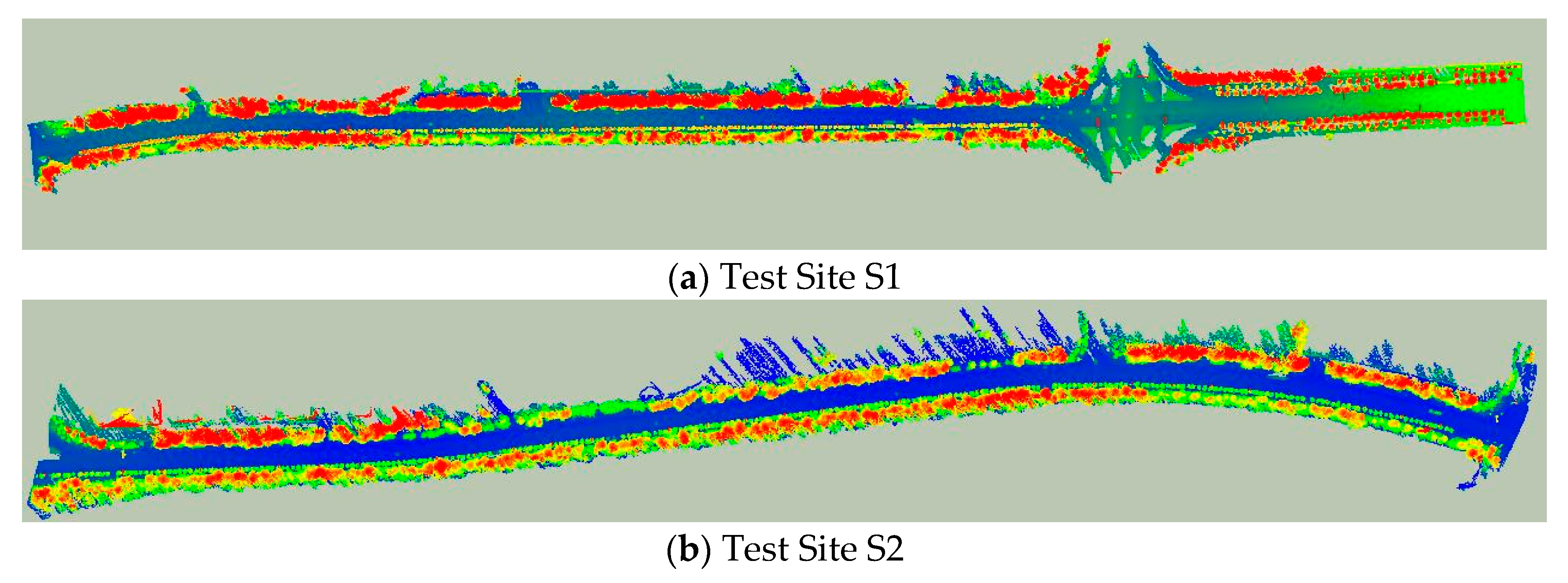
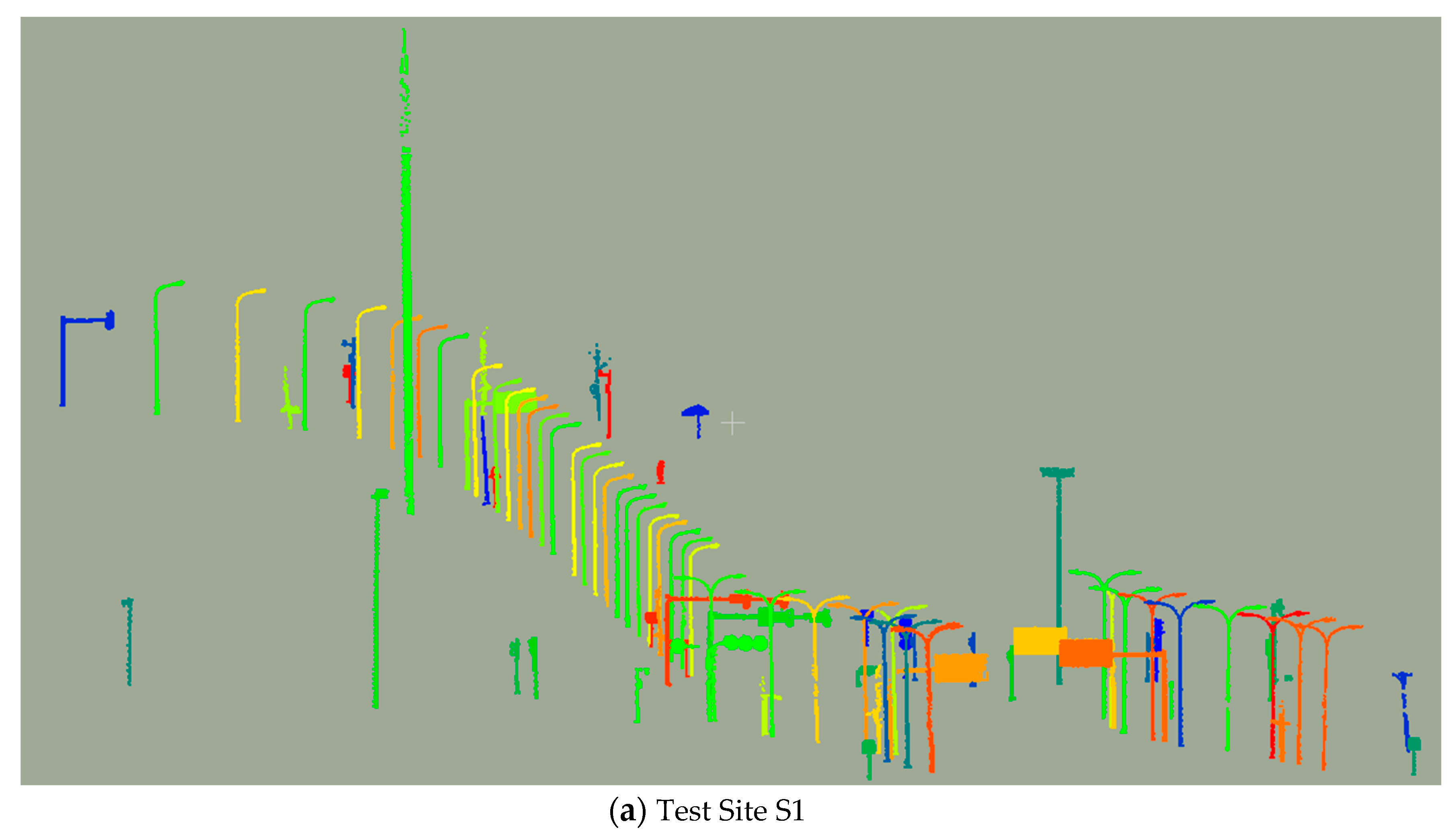
The overall view of the tested area is listed in Figure 7, where the points are coloured by height. Detailed information about the two test sites can be found in Table 1.

4.2. Parameter Settings

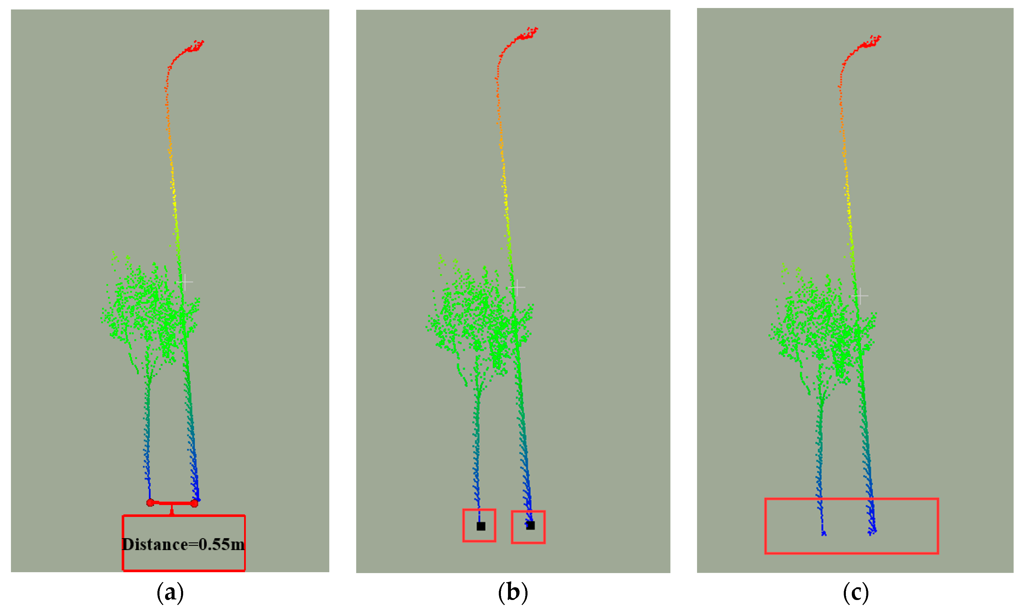
Table 2 depicted the parameter configuration of the proposed algorithm for the two test sites. vs. is the voxel size for the voxelization processing step which should be configured based on the average space between points [23]. For the scenes with large density variations, the voxel size should be configured based on the target road poles with low densities. The voxel size is configured as 0.3 m as the distance between points on the pole trunk of some road poles behind the first row of trees is nearly 0.3 m. As there may exist noisy points in the data, some points in the ring of the accumulative cylinders are also tolerable but the conditions should be strictly configured to select the correct target. The number of points in the ring area between two accumulative cylinders is configured as 4. The following five parameters in all depict the target objects that we are interested in. The target road pole radius should be less than 0.45 m; the target road pole should have a pole part with a height of at least 1.2 m and less than 4 points at its surrounding areas. Other researchers are recommended to first define their poles of interest and configure these corresponding parameters to obtain their targets. The threshold value r h 0 is found by analyzing hundreds of tree and pole clusters from real scenes. Detailed discussion about the threshold value selection can be found in our previous work [45]. Different parameter settings will affect the results in different ways. For example, the inner radius, outer radius and the cylinder height will affect the detection of road poles of different types. If we configure a bigger inner radius, the isolation analysis algorithm will detect poles with bigger radius. However, the space between poles are more restricted. In Figure 8, we present an example which depict the influence of different inner radius configurations on pole position detection results. When Ir is configured as 0.6m, the algorithm could detect poles with radius up to 0.6 m. But it could not detect poles that are within the distance of 0.6 m.

4.3. Results

4.3.1. Pre-Processing Results

The original point cloud dataset should be sectioned and voxelized first. The section length will affect the computational cost of the proposed method in a specific section. To section the experimental data into a number of blocks, we chose d = 100 m in dataset S1. In the other dataset, we chose d = 120 m because the dataset is flatter. Detailed discussion of section length configuration can be found in our previous work [46]. The following operations are all implemented on each block. Voxel size is a critical parameter in the following voxelization and localization step, which is mainly determined by point density. The density of the mobile laser scanning data in each test site varies greatly both between the test sites and within each test site. The average point span for distant objects in the test sites is approximately 0.15 m to guarantee that distant objects have vertically continuous voxels and the voxel size was configured as two times the average point span, namely, 0.3 m. The number of voxels after voxelization of S1 and S2 are 1,054,602 and 1,214,369, respectively, with a compression rate (1 − number of voxels containing data/number of original points) of 95.6% and 94.2%. After voxelization, the ground can be detected. The results for two selected blocks in each test site after back-projection from voxel to points are presented in Figure 9, where the green coloured points are detected ground points with the proposed method.

4.3.2. Results of Poles and Trees Localization

After filtering out the ground voxels, the localization step is then performed on the remaining voxel set, which produces trees and road pole centres. The key parameter configurations for selecting road poles and tree locations can be found in is configured as 0.6 m.
Two selected examples for locating trees and road poles are depicted in Figure 10, where the enlarged black points depicts the positions of the targets. It can be concluded from the figure that almost all target trees and road poles are accurately located.

4.3.3. Pole Detection Results

Two measures, completeness CP and correctness CR, are defined as follows:
C P = T P / A P
C R = T P / V P
where TP, AP and VP are the number of road poles belonging to (1) the correctly detected road poles using the proposed method, (2) the road poles collected by artificial visual interpretation and (3) the detected road poles using the proposed method, respectively. Table 3 depicts the results of two different test sites for different kinds of road poles, including lampposts, traffic signs, traffic lights and other poles, including utility poles and surveillance cameras. For the single class columns, the first number means the detected poles using the proposed method and the second number means the pole detected by visual inspection. The completeness and correctness of the whole class of road poles are computed using Equations (9) and (10). The last row in the table depict the average completeness (95.5%) and correctness (83.6%) of the two test sites, which is also calculated based on Equations (9) and (10). Two selected examples of the same area in Figure 10 are listed in Figure 11, in which the white coloured clusters are the extracted targets. The whole result for the two test sites is listed in Figure 12.

4.4. Performance Analysis of the Algorithm

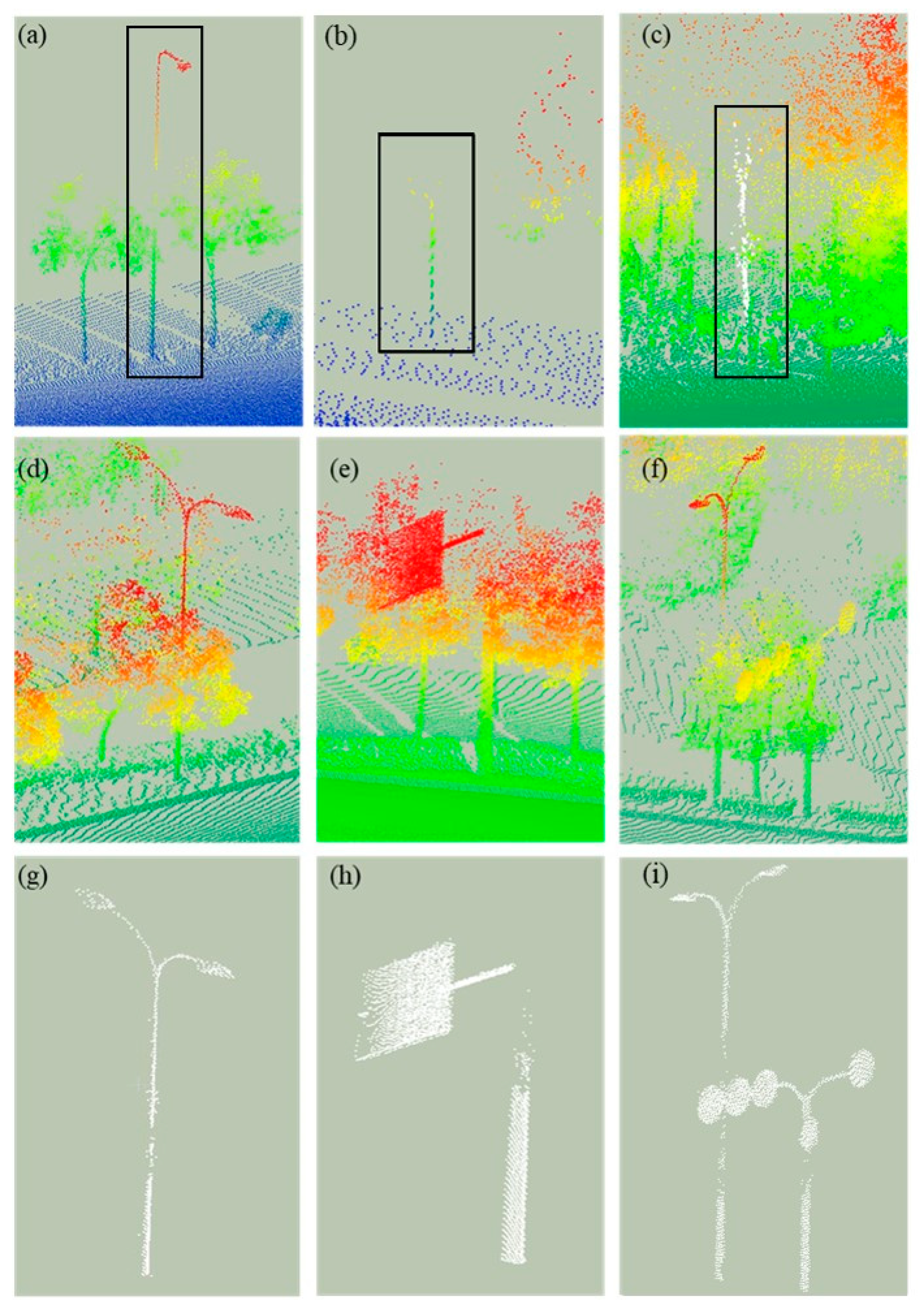
It can be concluded that the proposed method achieved high completeness values in both test areas but with low correctness values in test site S2. After deep inspection into the test sites, we found that the tree poles became bare poles because the leaves of the tree are occluded by the front trees, while the poles are reachable by the laser beams. The second line of Table 3 shows the quantitative results of test site S1. The actual number of lampposts, traffic signs, traffic lights and other poles were manually counted by visual inspection. In S1, 82 out of 86 poles were detected and 9 non-target objects were recognized as poles. In S2, 45 out of 47 poles were detected correctly and 16 non-pole furniture were incorrectly recognized as poles. All traffic signs were detected while other kinds of poles had some detection errors. Three lampposts were not detected because they were occluded and the vertical continuity was damaged by trees (Figure 13a). One traffic light and two other poles were not detected because they stand too far away from the laser scanners and the overall density is too small to be detected (Figure 13b). Most incorrectly detected non-targets with the proposed method came from those trees that stand behind the front row of trees, leaves were not scanned by the laser beams because of the occlusion while the poles were scanned (Figure 13c). These trees are presented in the dataset as bare poles or poles with branches and they almost fit our definition of poles. These errors can be eliminated by locating rows of trees, which will be one of our next research topics. The proposed method outperforms other pole extraction methods because it is robust when trees and poles are tangled together. Some examples of these situations are listed in the following figure. Figure 13d,e,f are the scenes in the original dataset and Figure 13g,h,i are the corresponding pole detection results with the proposed method. It can be seen that our method is able to detect and extract poles in these cluttered scenes where trees and poles are tangled or twisted with each other.

4.5. Comparison with Previous Methods

The comparison of different methods for detecting road poles is difficult to implement for several reasons: First of all, the target of each method may vary a lot as each method concentrate on specific class of road poles for their applications. For example, some researchers regard trees also as road poles [3,25] while others exclude trees in their detection of road poles [23,31]; Besides, no public dataset are found to utilize in related work to detect road poles; Thirdly, the proposed method concentrate on the cluttered scenes in urban scenes, which are not common scenes in other datasets but are common in our datasets. Therefore, theses cluttered scenes is not intensively studied in other researches and also make it difficult to compare the proposed method to state of art methods.
The recognition rate of the method by Golovinskiy et al. using segmentation based classification are 79% for short posts, 70% for lamp posts while only 58% for traffic signs and 52% for traffic lights [25]. Pu et al. experimented on the detection of road poles and achieved 86.9% detection rate for road poles. However this method were not applicable for connected road poles as they utilize connected component analysis algorithm to segment road poles. The algorithm from Cabo et al. also utilized the voxel based algorithm, the completeness and correctness values are 92.3% and 83.8 respectively [23]. The completeness and correctness values of the pole-like road furniture detection were higher than 90% in both the Enschede dataset and the Paris dataset in the method from Li et al. A recent research from Fan et al. on localization and detection of lamp posts achieve high detection rate with average value over 96% [31].
Although the direct comparison of different methods with different datasets is complicated, the detection rate of the proposed methods outperforms most the state of art methods (Table 3). The method from Wu et al reported higher detection rate of lamp posts than the proposed methods [31]. However, they did not concentrate on the detection of road poles in uneven mobile laser scanning data. Besides, they did some analysis on cluttered situations and showed the robustness of their method in situations where lamp post erect through trees (Figure 13d). However, for other more complex situations similar to Figure 13d,e, their method reported difficult to segment these poles out from these cluttered scenes.
Besides, the proposed method is more robust to point cloud dataset with density variations as we detect object locations in a three-dimensional way. The voxel size is configured as 0.3 m in our method to detect poles with point distances up to 0.3 m while the high density areas have points with distances less than 2 centimetres. Cabo et al.’s method perform isolation analysis in a two dimensional way which may not be robust when poles are far away from the laser scanners and have low point densities [23].

5. Conclusions

This paper proposes a three-phase approach to locate and extract road poles from MLS data. The original point cloud dataset is first sectioned and voxelized to compress and reorganize the original data and the ground voxels are detected based on the general assumptions of the flatness of the ground area. In the second stage, the locations of the poles and trees are located. The object centres are found as object locations based on the vertical continuity of the highest part of the objects. In the final stage, we focus on the poles in the cluttered segments. Poles in clutters are extracted by recognizing manmade structures.
There are plenty of streets in China with these tree-pole cluttered scenarios. Two datasets with such cluttered scenes were utilized in the experiments to test the validity of the proposed method. The proposed method proves to be robust in detecting kinds of road poles in most these scenarios and achieved over 95% accuracy for both datasets. The clustering method with the proposed definition of roughness makes it possible to segment out pole attachments in mobile laser scanning data when the attachments are even covered in tree leaves. Moreover, the proposed method only requires the coordinates of the point clouds to attain the anticipated results, which makes it applicable for more datasets. However, as stated in Section 4.4, many trees that were occluded by front trees were wrongly detected as poles, which led to less than 75% correctness value in the second dataset. This requires further study in our future research.

Author Contributions

Y.L., W.W., R.G. and X.L., contributed to the design and implementation of the proposed method, D.L. and W.X. helped collected the data, S.T., Z.Y. and Y.W. contributed to the analysis and processing the data, Y.L. wrote the article with input from all authors.

Funding

This study is funded by Open Fund of Key Laboratory of Urban Land Resources Monitoring and Simulation, Ministry of Land and Resources (KF-2018-03-066), the National Natural Science Foundation of China (41801392), the China Postdoctoral Science Foundation (2018M633133, 2018M640821 and 2018M643150), Special fund for the development of strategic emerging industries in Shenzhen (JSGG20170412170711532), Research on Key Technology for Scenario Construction of Severe Urban Disasters and Emergency Drill System (JYCJ20170412142239369) and Research on Emergency Technology of Monitoring and Forecasting Geological Disaster Using Big Data(JCYJ20170412142144518).

Conflicts of Interest

The authors declare no conflict of interest.

References

  1. Pu, S.; Vosselman, G. Automatic extraction of building features from terrestrial laser scanning. Int. Arch. Photogramm. Remote Sens. Spatial Inf. Sci. 2006, 36, 25–27. [Google Scholar]
  2. Pu, S.; Rutzinger, M.; Vosselman, G.; Oude Elberink, S. Recognizing basic structures from mobile laser scanning data for road inventory studies. ISPRS J. Photogramm. Remote Sens. 2011, 66, S28–S39. [Google Scholar] [CrossRef]
  3. Li, L.; Li, Y.; Li, D. A method based on an adaptive radius cylinder model for detecting pole-like objects in mobile laser scanning data. Remote Sens. Lett. 2016, 7, 249–258. [Google Scholar] [CrossRef]
  4. Brenner, C. Extraction of Features from Mobile Laser Scanning Data for Future Driver Assistance Systems. Lect. Notes Geoinf. Cartogr. 2009. [Google Scholar] [CrossRef]
  5. Brenner, C. Global localization of vehicles using local pole patterns. In Pattern Recognition; Springer: Berlin, Germany, 2009; pp. 61–70. [Google Scholar]
  6. Lehtomäki, M.; Jaakkola, A.; Hyyppä, J.; Lampinen, J.; Kaartinen, H.; Kukko, A.; Puttonen, E.; Hyyppä, H. Object classification and recognition from mobile laser scanning point clouds in a road environment. IEEE Trans. Geosci. Remote Sens. 2016, 54, 1226–1239. [Google Scholar] [CrossRef]
  7. Liang, X.; Litkey, P.; Hyyppa, J.; Kaartinen, H.; Vastaranta, M.; Holopainen, M. Automatic Stem Mapping Using Single-Scan Terrestrial Laser Scanning. IEEE Trans. Geosci. Remote Sens. 2012, 50, 661–670. [Google Scholar] [CrossRef]
  8. Huang, P.; Cheng, M.; Chen, Y.; Luo, H.; Wang, C.; Li, J. Traffic Sign Occlusion Detection Using Mobile Laser Scanning Point Clouds. IEEE Trans. Intell. Transp. Syst. 2017, 1–13. [Google Scholar] [CrossRef]
  9. Raumonen, P.; Kaasalainen, M.; Åkerblom, M.; Kaasalainen, S.; Kaartinen, H.; Vastaranta, M.; Holopainen, M.; Disney, M.; Lewis, P. Fast Automatic Precision Tree Models from Terrestrial Laser Scanner Data. Remote Sens. 2013, 5, 491–520. [Google Scholar] [CrossRef] [Green Version]
  10. Elberink, S.O.; Khoshelham, K. Automatic Extraction of Railroad Centerlines from Mobile Laser Scanning Data. Remote Sens. 2015, 7, 5565–5583. [Google Scholar] [CrossRef] [Green Version]
  11. Jochem, A.; Höfle, B.; Rutzinger, M. Extraction of Vertical Walls from Mobile Laser Scanning Data for Solar Potential Assessment. Remote Sens. 2011, 3, 650–667. [Google Scholar] [CrossRef]
  12. Kaasalainen, S.; Jaakkola, A.; Kaasalainen, M.; Krooks, A.; Kukko, A. Analysis of incidence angle and distance effects on terrestrial laser scanner intensity: Search for correction methods. Remote Sens. 2011, 3, 2207–2221. [Google Scholar] [CrossRef]
  13. Lehtomäki, M.; Jaakkola, A.; Hyyppä, J.; Kukko, A.; Kaartinen, H. Detection of Vertical Pole-Like Objects in a Road Environment Using Vehicle-Based Laser Scanning Data. Remote Sens. 2010, 2, 641–664. [Google Scholar] [CrossRef] [Green Version]
  14. Yokoyama, H.; Date, H.; Kanai, S.; Takeda, H. Detection and Classification of Pole-like Objects from Mobile Laser Scanning Data of Urban Environments. Int. J. CAD/CAM 2013, 13, 31–40. [Google Scholar]
  15. Yang, B.; Zhen, D. A shape based segmentation method for mobile laser scanning point clouds. ISPRS J. Photogramm. Remote Sens. 2013, 81, 19–30. [Google Scholar] [CrossRef]
  16. Yang, B.; Dong, Z.; Zhao, G.; Dai, W. Hierarchical extraction of urban objects from mobile laser scanning data. ISPRS J. Photogramm. Remote Sens. 2015, 99, 45–57. [Google Scholar] [CrossRef]
  17. Wu, B.; Yu, B.; Yue, W.; Shu, S.; Tan, W.; Hu, C.; Huang, Y.; Wu, J.; Liu, H. A Voxel-Based Method for Automated Identification and Morphological Parameters Estimation of Individual Street Trees from Mobile Laser Scanning Data. Remote Sens. 2013, 5, 584–611. [Google Scholar] [CrossRef] [Green Version]
  18. Rodríguez-Cuenca, B.; García-Cortés, S.; Ordóñez, C.; Alonso, M. Automatic Detection and Classification of Pole-Like Objects in Urban Point Cloud Data Using an Anomaly Detection Algorithm. Remote Sens. 2015, 7, 12680–12703. [Google Scholar] [CrossRef] [Green Version]
  19. Zhang, C.; Zhou, Y.; Qiu, F. Individual Tree Segmentation from LiDAR Point Clouds for Urban Forest Inventory. Remote Sens. 2015, 7, 7892–7913. [Google Scholar] [CrossRef] [Green Version]
  20. Li, F.; Elberink, S.O.; Vosselman, G. Pole-Like Street Furniture Decompostion in Mobile Laser Scanning Data. ISPRS Ann. Photogramm. Remote Sens. Spat. Inf. Sci. 2016, 3, 193–200. [Google Scholar] [CrossRef]
  21. Li, F.; Oude Elberink, S.; Vosselman, G. Pole-Like Road Furniture Detection and Decomposition in Mobile Laser Scanning Data Based on Spatial Relations. Remote Sens. 2018, 10, 531. [Google Scholar] [Green Version]
  22. Li, F.; Elberink, S.O.; Vosselman, G. Semantic labelling of road furniture in mobile laser scanning data. Int. Arch. Photogramm. Remote Sens. Spat. Inf. Sci. 2017, 42, 247–254. [Google Scholar] [CrossRef]
  23. Cabo, C.; Ordóñez, C.; García-Cortés, S.; Martínez, J. An algorithm for automatic detection of pole-like street furniture objects from Mobile Laser Scanner point clouds. ISPRS J. Photogramm. Remote Sens. 2014, 87, 47–56. [Google Scholar] [CrossRef]
  24. El-Halawanya, S.I.; Lichtia, D.D. Detecting road poles from mobile terrestrial laser scanning data. GISci. Remote Sens. 2013, 50, 704–722. [Google Scholar] [CrossRef]
  25. Golovinskiy, A.; Kim, V.G.; Funkhouser, T. Shape-based Recognition of 3D Point Clouds in Urban Environments. In Proceedings of the International Conference on Computer Vision (ICCV), Kyoto, Japan, 29 September–2 October 2009; pp. 2154–2161. [Google Scholar]
  26. Lai, K.; Fox, D. Object Recognition in 3D Point Clouds Using Web Data and Domain Adaptation. Int. J. Robot. Res. 2010, 29, 1019–1037. [Google Scholar] [CrossRef] [Green Version]
  27. Ishikawa, K.; Tonomura, F.; Amano, Y.; Hashizume, T. Recognition of Road Objects from 3D Mobile Mapping Data. Int. J. CAD/CAM 2013, 13, 41–48. [Google Scholar]
  28. Wang, J.; Lindenbergh, R.; Menenti, M. SigVox—A 3D feature matching algorithm for automatic street object recognition in mobile laser scanning point clouds. ISPRS J. Photogramm. Remote Sens. 2017, 128, 111–129. [Google Scholar] [CrossRef]
  29. Oude Elberink, S.; Kemboi, B. User-assisted object detection by segment based similarity measures in mobile laser scanner data. ISPRS-Int. Arch. Photogramm. Remote Sens. Spat. Inf. Sci. 2014, 3, 239–246. [Google Scholar] [CrossRef]
  30. Zhou, Y.; Wang, D.; Xie, X.; Ren, Y.; Li, G.; Deng, Y.; Wang, Z. A Fast and Accurate Segmentation Method for Ordered LiDAR Point Cloud of Large-Scale Scenes. IEEE Geosci. Remote Sens. Lett. 2014, 11, 1981–1985. [Google Scholar] [CrossRef]
  31. Wu, F.; Wen, C.; Guo, Y.; Wang, J.; Yu, Y.; Wang, C.; Li, J. Rapid Localization and Extraction of Street Light Poles in Mobile LiDAR Point Clouds: A Supervoxel-Based Approach. IEEE Trans. Intell. Transp. Syst. 2017, 18, 292–305. [Google Scholar] [CrossRef]
  32. Golovinskiy, A.; Funkhouser, T. Min-cut based segmentation of point clouds. In Proceedings of the IEEE 12th International Conference on Computer Vision Workshops (ICCV Workshops), Kyoto, Japan, 27 September–4 October 2009; pp. 39–46. [Google Scholar]
  33. Yu, Y.; Li, J.; Guan, H.; Wang, C.; Yu, J. Semiautomated Extraction of Street Light Poles from Mobile LiDAR Point-Clouds. IEEE Trans. Geosci. Remote Sens. 2015, 53, 1374–1386. [Google Scholar] [CrossRef]
  34. Li, Y.; Li, L.; Li, D.; Yang, F.; Liu, Y. A Density-Based Clustering Method for Urban Scene Mobile Laser Scanning Data Segmentation. Remote Sens. 2017, 9, 331. [Google Scholar] [CrossRef]
  35. Toth, C.; Paska, E.; Brzezinska, D. Using road pavement markings as ground control for lidar data. Int. Arch. Photogramm. Remote Sens. Spat. Inf. Sci. 2008, 37, 189–195. [Google Scholar]
  36. Yang, B.; Fang, L.; Li, Q.; Li, J. Automated extraction of road markings from mobile lidar point clouds. Photogramm. Eng. Remote Sens. 2012, 78, 331–338. [Google Scholar] [CrossRef]
  37. Yang, B.; Fang, L.; Li, J. Semi-automated extraction and delineation of 3D roads of street scene from mobile laser scanning point clouds. ISPRS J. Photogramm. Remote Sens. 2013, 79, 80–93. [Google Scholar] [CrossRef]
  38. Guan, H.; Li, J.; Yu, Y.; Wang, C.; Chapman, M.; Yang, B. Using mobile laser scanning data for automated extraction of road markings. ISPRS J. Photogramm. Remote Sens. 2014, 87, 93–107. [Google Scholar] [CrossRef]
  39. Kumar, P.; McElhinney, C.P.; Lewis, P.; McCarthy, T. An automated algorithm for extracting road edges from terrestrial mobile LiDAR data. ISPRS J. Photogramm. Remote Sens. 2013, 85, 44–55. [Google Scholar] [CrossRef] [Green Version]
  40. Chen, D.; He, X. Fast automatic three-dimensional road model reconstruction based on mobile laser scanning system. Opt.-Int. J. Light Electron Opt. 2015, 126, 725–730. [Google Scholar] [CrossRef]
  41. Riveiro, B.; González-Jorge, H.; Martínez-Sánchez, J.; Díaz-Vilariño, L.; Arias, P. Automatic detection of zebra crossings from mobile LiDAR data. Opt. Laser Technol. 2015, 70, 63–70. [Google Scholar] [CrossRef]
  42. Rodríguez-Cuenca, B.; García-Cortés, S.; Ordóñez, C.; Alonso, M.C. An approach to detect and delineate street curbs from MLS 3D point cloud data. Autom. Constr. 2015, 51, 103–112. [Google Scholar] [CrossRef]
  43. Ordóñez, C.; Cabo, C.; Sanz-Ablanedo, E. Automatic Detection and Classification of Pole-Like Objects for Urban Cartography Using Mobile Laser Scanning Data. Sensors 2017, 17, 1465. [Google Scholar] [CrossRef]
  44. Demantké, J.; Mallet, C.; David, N.; Vallet, B. Dimensionality based scale selection in 3D lidar point clouds. Int. Arch. Photogramm. Remote Sens. Spat. Inf. Sci. 2012, 3812, 97–102. [Google Scholar]
  45. Li, L.; Li, D.; Zhu, H.; Li, Y. A dual growing method for the automatic extraction of individual trees from mobile laser scanning data. ISPRS J. Photogramm. Remote Sens. 2016, 120, 37–52. [Google Scholar] [CrossRef]
  46. Li, L.; Zhang, D.; Ying, S.; Li, Y. Recognition and Reconstruction of Zebra Crossings on Roads from Mobile Laser Scanning Data. ISPRS Int. J. Geo-Inf. 2016, 5, 125. [Google Scholar] [CrossRef]
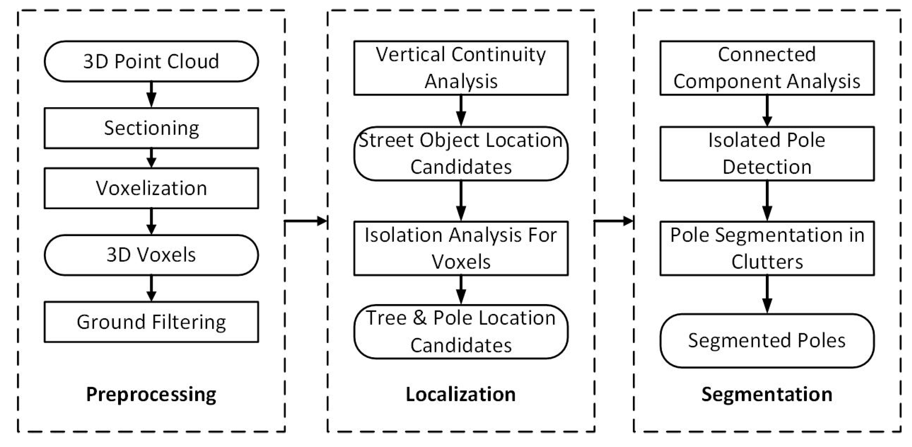
Figure 1. Workflow of the proposed method.
Remotesensing 11 00401 g001
Figure 2. Sectioning point cloud data.
Remotesensing 11 00401 g002
Figure 3. Examples of two scenes using the proposed density measurement.
Remotesensing 11 00401 g003
Figure 4. An isolation analysis example for voxels.
Remotesensing 11 00401 g004
Figure 5. Roughness distributions of two isolated point cloud clusters. (a) The roughness value distribution of the tree points. (b) Sectioning the tree to upper part and lower part. (c) Three sections from the upper part of the tree and the average roughness value (rh) of each section. (d) The roughness value distribution of the lamppost points. (e) Sectioning the lamppost to upper part and lower part. (f) Three sections from the upper part of the lamppost and the average roughness value (rh) of each section.
Remotesensing 11 00401 g005
Figure 6. Road pole detection in two typical cluttered scenes: (a) The cluster of a cluttered scene with point coloured by height. (b) Detected pole part by vertical growing algorithm from (a). (c) One detected manmade structure by region growing based on roughness from (a). (d) United detection result of pole part and manmade structure from (a). (e) Another cluster of a cluttered scene with point coloured by height. (f) Detected pole parts by vertical growing algorithm from (e). (g) Two detected manmade structures by region growing based on roughness from (e). (h) United detection result of the pole part and manmade structure from (e).
Remotesensing 11 00401 g006
Figure 7. Overall view of the two test sites.
Remotesensing 11 00401 g007
Figure 8. Parameter setting example. (a) Original cluster with two street object whose horizontal distance between them is 0.55 m. (b) Pole candidate position detection result with two positions detected when Ir is configured as 0.45 m. (c) Pole candidate position detect result with no position detected when Ir is configured as 0.6m.
Remotesensing 11 00401 g008
Figure 9. Selected results of ground detection.
Remotesensing 11 00401 g009
Figure 10. Resulting samples of localization of trees and road poles.
Remotesensing 11 00401 g010
Figure 11. Result samples of detected road poles in two selected scenes.
Remotesensing 11 00401 g011
Figure 12. Pole extraction results of the two test sites.
Remotesensing 11 00401 g012aRemotesensing 11 00401 g012b
Figure 13. Sample results: (a) A lamppost undetected because of occlusion; (b) A lamppost undetected because of low density; (c) A lamppost undetected because of front tree occlusion; (d) A lamppost in a cluttered scene; (e) A traffic sign in a cluttered scene; (f) A lamppost and a traffic sign in a cluttered scene; (g) Detection result of (d); (h) Detection result of (e); (i) Detection result of (f).
Remotesensing 11 00401 g013
Table 1. Description of the test sites.
Test SitesLength (m)Width (m)Points (million)Average Density (points/m2)
S114006023.6445
S212005020.7345
Table 2. Parameter settings applied to our two test sites.
NameValuesDescription
VS0.3 mVoxel size
Ir1.5 (0.45 m)Inner radius
Or3 (0.9 m)Outer radius
NP4Number of points allowed in the ring of the concentric cylinder
NV1Number of voxels allowed in the ring of the concentric cylinder
L4 (1.2 m)The height of the cylinder
r h 0 0.07The threshold value of roughness that separate tree crowns from poles
Table 3. Detection results in the test sites.
Test SitesLamp PostsTraffic SignsTraffic LightsOther PolesCompletenessCorrectness
S145/4715/1512/1312/1382/86 (95.3%)82/91 (90.1%)
S236/376/61/12/345/47 (95.7%)45/61 (73.8%)
Average95.5%83.6%