Abstract
There has been a growing concern for the urbanization induced local warming, and the underlying mechanism between urban thermal environment and the driving landscape factors. However, relatively little research has simultaneously considered issues of spatial non-stationarity and seasonal variability, which are both intrinsic properties of the environmental system. In this study, the newly proposed multi-scale geographically weighted regression (MGWR) is employed to investigate the seasonal variations of the spatial non-stationary associations between land surface temperature (LST) and urban landscape indicators under different operating scales. Specifically, by taking Wuhan as a case study, Landsat-8 images were used to achieve the LSTs in summer, winter and the transitional season, respectively. Landscape composition indicators including fractional vegetation cover (FVC), albedo and water percentage (WP) and urban morphology indicators covering building density (BD), building height (BH) and building volume density (BVD) were employed as potential landscape drivers of LST. For reference, the conventional geographically weighted regression (GWR) and ordinary least squares (OLS) regression were also employed. Results revealed that MGWR outperformed GWR and OLS in terms of goodness-of-fit for all seasons. For the specific associations with LST, all six indicators exhibited evident seasonal variations, especially from the transition season to winter. FVC, albedo and BD were observed to possess great spatial non-stationarity for all seasons, while WP, BH and BD tended to influence LST globally. Overall, FVC exhibited certain positive effect in winter. The negative effect of WP was the greatest among all indicators, although it became the weakest in winter. Albedo tended to influence LST more complicatedly than simple cooling. BD, with a consistent heating effect, was testified to have a greater influence on LST than BH for all seasons. The BH-LST association tended to transfer into positive in winter, while the BVD-LST association remained negative for all seasons. The results could support the establishment of season- and site-specific mitigation strategies. Generally, this study facilitates our understanding of human-environment interaction and narrows the gap between climate research and city management.
1. Introduction
Urbanization induced local warming has aroused wide academic attention for its significance on urban climatology, human–environment interaction and urban sustainability [1]. It has been repeatedly proven that urbanization deteriorates the urban thermal environment through the continuous replacement of natural land cover with artificial surface [2,3,4,5], as it alters the thermal properties of the land, the energy exchange regime and atmospheric circulation characteristics [6]. The evident warming trend has contributed to a variety of environmental problems, including biodiversity decrease, and water and air quality deterioration [7]. The synthesized consequences further exert a dramatic impact on human health and well-being, and may potentially increase cause-specific morbidity and mortality [8]. Land surface temperature (LST) derived from satellite remotely sensed thermal infrared (TIR) imagery has become an indispensable indicator for urban thermal environment study as being advantageous in full spatial coverage and multiple temporal scales compared to air temperatures collected from weather stations [9,10,11,12]. Studies characterizing the spatial and temporal patterns of LST are well documented, however, the effective mitigation of excessive urban heat demands further knowledge about how LST is impacted by potential land surface drivers [13,14]. As a result, numerous studies have examined the associations between landscape indicators and LST [15,16,17,18,19,20], so as to generate useful knowledge about how the urban physical form interacts with the climatic context to support further climate-sensitive planning. On the whole, the analysis of the urban landscape and LST association has demonstrated three significant tendencies in consideration of the seasonal variation and spatial non-stationarity of the association, and a prominent growth in sophistication regarding the explanatory variables used for regression.
Seasonal analysis of urban landscape and LST association has recently emerged from the previous summer-biased literature given the temporal non-stationarity of the association, although such studies were still inclined to apply global models for regression. The LST dynamic is not temporally constant as solar thermal radiation, hydrothermal condition and spatial characteristics of vegetation coverage tend to vary seasonally [14,21]. Such variability is deemed to have an impact on the effectiveness of climate adaptation strategies [21,22]. In fact, the inconsistent influences of driving forces in different seasons have been revealed in multiple studies [14,21,23,24]. Nevertheless, the majority of previous studies applied only one snapshot to identify the impact of landscape indicators on LST [15,16,25,26,27,28] with a summer-biased manner [7,21]. Namely, summer tends to dominate all single- and multi-season studies with the largest proportion of 33% according to a new systematic review of LST studies since its origin in 1972 [7]. Specifically for single-season literature, summer occupies 60% for its extreme heat climate and the accompanying remarkable adverse impact [7]. Knowledge drawn from such a static point of view can be misleading given the complexity of urban climatology [5]. Several studies exclusively explored such seasonal contrast of the association to highlight the significance of seasonal non-stationarity using global analysis tools [14,21,24]. For example, Peng et al. [14] explored the dominant factors influencing the spatial variations of LST in different seasons in Shenzhen, China. Among the 17 indictors considered, the specific results [14] indicate that the normalized difference build-up index (NDBI), the normalized difference vegetation index (NDVI), the construction land percentage and NDVI are respectively the most important indicators affecting the spatial heterogeneity of LST in summer, the transition season and winter. Chun and Guildmann [21] revealed that the increase of greenery in Columbus, Ohio could result in conflicting consequences respectively in summer and winter, with a cooling effect in the former and heating in the latter. As a result, the consideration of the seasonal effects of the LST dynamic is essential for climate-sensitive land-use policies to achieve year-long effectiveness.
Spatial non-stationarity has also been a new focus of the urban landscape-LST exploration with the introduction and application of the geographically weighted regression (GWR) [29]. As a common nature of geographical processes [30,31,32], spatial non-stationarity, namely the association tends to vary geographically, has been detected in multiple geographical environmental phenomena [33,34,35,36]. Unlike physical processes, which are stationary, geographical environmental processes tend to be spatially non-stationary as the driving natural or anthropogenic factors are changing over space, thus may play different roles in different areas [35]. As a result, the measurement of such environmental association to a certain extent depends on where the measurement is taken [29]. Conventional global regression models are limited in such environmental studies as they assume the associations to be constant over space. For an urban study, cities are treated holistically and specific information on the intra-city scale is inevitably neglected. In urban thermal research, multiple studies have utilized GWR to model the static associations between landscape indicators and LST using only one snapshot [36,37,38,39,40]. Results reveal that the application of global models, such as the ordinary least squares (OLS), can result in underestimation of the urban heat island (UHI) intensity when it comes to prediction [38], hence promotes the possibility of underestimating health risk towards heat stress. GWR, on one hand, is able to characterize heterogeneity in processes by allowing the associations to vary across space, on the other hand, it conforms to Tobler’s first law of geography [41] as it borrows nearby locations and weights them according to distance to calibrate the prediction of any specific point [29,42]. As a result, GWR can uncover more comprehensive knowledge about the associations while achieving a better regression coefficient. Besides, the localized regression coefficient is also able to provide unique information for site-specific mitigation from urban design and planning [12,40,43].
The newly proposed multi-scale geographically weighted regression (MGWR) [42] can be a more effective tool to explore the non-stationary dynamics of LST, as it is superior to GWR for allowing the process to operate not only locally but also at varying spatial scales. The classical GWR model is inflexible as it assumes all processes to be operated at the same spatial scale with one optimal bandwidth in multivariate regression [32,42]. In reality, different natural processes may exhibit diversified levels of spatial non-stationarity, some may possess no non-stationarity at all when the study scope is small [37]. In contrast, MGWR allows each process to be specified with its own spatial scale in an intuitive manner [42]. In fact, scale is a pivotal issue for all science [44,45], especially for geographical information science [46,47]. In urban thermal environment research, multiple categories of landscape indicators are normally encompassed in modeling to uncover the complicated underlying mechanism. However, all processes may not necessarily operate under a consistent spatial scale. For example, biophysical and urban morphological indicators respectively extracted from Landsat images and building survey data may impact the urban thermal environment under different spatial scales. As a result, the MGWR can be a superior tool to explore the locally varied associations between LST and the urban landscape.
Along with the exponential development of urban thermal environment studies and the accompanying growth in sophistication regarding the consideration of explanatory variables, urban morphology has been included into the LST dynamic investigation for mitigation efficiency. To translate interaction knowledge between the physical form and the climatic context into practical planning applications, so as to effectively mitigate the local warming trend, has always been significant and yet challenging [48]. As a result, it is crucial to take the efficiency of being regulated through urban planning into consideration while selecting landscape driving forces of LST. Urban morphology which is broadly examined to be significantly correlated with LST is thus advantageous as it corresponds directly to the domain of urban design and planning [49,50,51]. Urban morphology mainly impacts LST through the alteration of surface albedo and air ventilation [28,50]. The broadly employed indicators include building density (BD), building height (BH), building volume density (BVD) and sky view factor (SVF) [22,28,49,50]. For LST dynamic study, it has been common practice to utilize landscape composition or configuration indicators for city-wide analysis [16,52,53]. Specifically, landscape composition, which illustrates the quantity and proportion of land cover features generally covers land cover proportion and biophysical descriptor obtained from spectral indices or a spectral unmixing technique [19]. Landscape configuration refers to the spatial characteristics of individual areas and spatial relationships among them [14,18]. The few studies incorporating urban morphology into consideration [17,21,28] are still limited as global analysis tools are utilized, thus neglecting the intrinsic spatial non-stationarity of the associations. In the future, it is significant to apply local regression tools, such as MGWR, to explore the spatial non-stationary association between LST and urban morphology. It can also be worthwhile to exclusively investigate the operating scale difference between the associations with urban morphology, and landscape composition or configuration.
Given the above background, this study intends to introduce MGWR to investigate the seasonal variations of the spatial non-stationary associations among LST and multiple urban landscape indicators. The aims of this study are to (1) compare the spatial patterns of LST in different seasons; (2) select landscape indicators which illustrate the LST dynamic, and also support regulation from urban planning effectively; (3) model and evaluate the associations between LST and landscape indicators through OLS, GWR and MGWR; and (4) analyze the seasonal variations of the spatial non-stationary associations modeled by MGWR.
2. Study Area and Data Sets
2.1. Wuhan, China
Wuhan, a megacity located in central China, is selected as a case study to investigate the urban thermal dynamic in growing high-density cities. Wuhan ranks as the 5th largest city in China with a population over 10 million. The total area of the city is about 8500 km2, among which 888 km2 is a built-up area in 2013 and 1992 km2 for 2018. Wuhan exhibits a typical subtropical monsoon climate with abundant solar radiation and rainfall. Specifically, summer dominants as the longest period of almost 135 days a year, followed by winter of about 110 days and the transition season covering spring and autumn of a total 120 days [54]. Wuhan has witnessed massive urbanization during the last two decades, which has evidently deteriorated its thermal environment [5]. It is still under burden of such risk for the next decade as the city is targeted to be a national central city by the National Development and Reform Commission (NDRC). The urban thermal dynamic exploration of Wuhan will contribute to the minimization of unwanted aspects and maximization of beneficial ones of the developing process. As presented in Figure 1 with a Landsat 8 image collected on 16th August 2013, a 39.0 km × 31.5 km area, which covers the central downtown and the large expansion areas of the city was selected for the specific study. The study area was also sufficient to illustrate the heterogeneity of land cover with diversified water bodies, vegetation areas and built-up areas with different levels of intensity. The upper-left and lower-right coordinates are 30°44′26″N, 114°12′01″E and 30°26′47″N, 114°35′46″E.
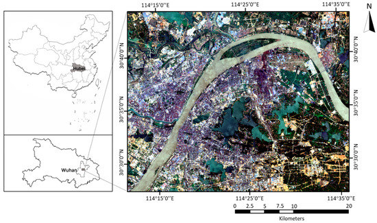
Figure 1.
The study area represented by the Landsat 8 image (RGB) acquired on 16 August 2013.
2.2. Data Sets
Landsat 8 images and building survey data of three seasons spanning from 2013 to 2014 were utilized in this study. Due to cloud contamination induced data deficiency and the relative similar LST patterns of spring and autumn in Wuhan [5,12], a three-season division approach, covering summer, transition season and winter, was utilized referring to the season delineation for LST seasonal analysis in Hong Kong [55] and Shen Zhen [14]. In fact, spring and autumn are evidently shorter than summer and winter in Wuhan with a total averaged 120 days a year [54], hence, it is acceptable to combine spring and autumn into transition season. Specifically, three cloud-free Landsat 8 images respectively acquired on 16 August 2013, 3 October 2013 and 23 January 2014 were employed to retrieve LSTs and landscape composition indicators of typical summer, transition season and winter of Wuhan. The three corresponding days for image acquisition experienced no precipitation on the very days and also the two days before. Besides, building survey data of 2013 and 2014 provided by the Land Resources and Planning Information Center of Wuhan were utilized to retrieve urban morphology indicators.
3. Methodology
The methodology developed in this study followed a workflow for the seasonal analysis of the spatial non-stationary associations between LST and landscape indicators. The methodological framework included three main steps, as presented in Figure 2: (1) Retrieve the LSTs from Landsat 8 thermal infrared sensor (TIRS) images and analyze the corresponding spatial patterns in different seasons (Section 3.1). (2) Obtain landscape composition and urban morphology indicators respectively from Landsat 8 images and building survey data (Section 3.2). (3) Model the associations between LST and landscape indicators through OLS, GWR and MGWR, evaluate the behavior of the three models and analyze the seasonal variation of the spatial non-stationary associations modelled by MGWR (Section 3.3).
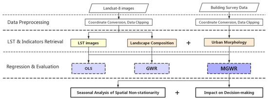
Figure 2.
The methodological framework used in this study.
3.1. The Retrieval of LST
The classic radiative transfer equation (RTE) [56,57] was employed to retrieve the LST from the selected Landsat 8 TIRS scenes. It is recommended by the United States Geological Survey (USGS) to merely use the Band 10 of Landsat 8 TIRS data to retrieve LST due to the larger calibration uncertainty associated with Band 11 (https://www.usgs.gov/land-resources/nli/landsat/landsat-8-data-users-handbook). In the study of Yu et al. [57] to compare multiple methods for LST retrieval from Landsat 8, RTE-based method using band 10 was validated to produce LST data with superior accuracy of Root Mean Square Error (RMSE) being lower than 1 K [57], where RMSE is common measure for the imperfection of numerical predictions. The RTE algorithm was thus utilized to retrieve LST from the radiometrically corrected data through:
where denotes the at-sensor radiance, ɛ is land surface emissivity, represents the ground blackbody radiance decided by Planck’s law and denotes LST. and respectively represent the downwelling and upwelling atmospheric radiances, is atmospheric transmittance. Furthermore, LST can be calculated as:
where λ is the effective band wavelength, = 14387.7 μm, . The atmospheric correction parameter calculator (https://atmcorr.gsfc.nasa.gov/) provided by National Aeronautics and Space Administration (NASA) was used to calculate the downwelling and upwelling atmospheric radiance [58].
3.2. The Selection and Retrieval of Landscape Indicators
Ten landscape indicators were preliminarily selected for a multicollinearity test according to the efficiency of illustrating LST dynamic and being regulated through urban planning. The landscape composition indicators derived from Landsat images cover NDVI [14,15,19,40,53], fractional vegetation cover (FVC) [59,60], NDBI [14,15,19,53], impervious surface fraction (ISF) [26,27,40], surface albedo [61,62] and water percentage (WP) [14,16,26,52]. All biophysical indicators were retrieved after atmospheric correction. Vegetation, which possesses great sense for temperature mitigation, has been broadly examined to be strongly correlated to LST [14,15,19,40,53,59,60]. Hence, it is significant to explore the spatial non-stationary association between vegetation and LST and the corresponding seasonal variations. Remote sensed biophysical vegetation indexes are recommendable as tested to be correlated with LST on a level higher than land cover proportional vegetation index [19]. Considering the great impact of multicollinearity on the accuracy of multivariate regression [63], two vegetation indices, NDVI and FVC were prepared for screening. The index with a smaller and tolerable multicollinearity with other indicators could be reserved for further modeling. WP, which is derived from the modified normalized difference water index (MNDWI) of each season, was utilized to represent water coverage. Compared to MNDWI, WP is a more easily visualized indicator with equal correlation with LST [19]. For the original biophysical water index characterization, MNDWI is superior to NDWI (normalized difference water index) as the latter tends to extract water cover integrated with construction land features [14]. The urban morphology indicators calculated from building survey data contain BD, BH, BVD and SVF [22,28,49,50]. The description and data range of the selected landscape composition and urban morphology indicators are presented in Table 1. The multicollinearity among the indicators was examined using the variance inflation factor (VIF), which directly indicates the impact of collinearity on the estimation precision of the slope coefficient [63]. Referring to previous studies [40,64,65,66], a matching with tolerable multicollinearity (VIF < 10) was identified as the final indicator system for later modeling in this study.

Table 1.
Comprehensive information about the selected indicators.
All variables are resampled to the city block scale of 500 m in urban climatology research [70], as identified by multiple related studies to be the optimal spatial scale for exploring LST and landscape association in Wuhan [27,71]. The city block scale is also recommendable for city-scale study as it is the smallest urban unit where homogeneity is possible while also large enough to generate localized breeze systems [70]. Specifically, the resampling was implemented through the Pixel Aggregation tool provided by Exelis ENVI, as recommended by multiple studies [25,27,72]. The tool aggregates the pixel values that contribute to the output pixel in a weighted averaging manner, hence, the influence of neighboring pixels is eliminated [27,72].
3.3. Regression Modeling and Evaluation
The associations between LST and the selected indicators are quantified through OLS, GWR and MGWR. The localized contribution of each indicator to LST is quantified through the corresponding slope coefficients derived from the models. Specifically, OLS is a global regression model, which has been commonly used as a benchmark model to compare with improved models [38,40]. It can be expressed as:
where denotes LST, represents the th indicators considered, is the intercept value, represents the number of indicators, denotes slope coefficient and is the random error term.
GWR [29], the most popular spatially varying coefficient (SVC) model by far [32], is an extension of the conventional regression framework, which allows the model parameters to vary in space. Hence, it breaks through the unrealistic hypothesis supported by conventional models in geoscience that the association between dependent and independent variables is constant over space [40]. GWR has been broadly proved to outperform OLS in terms of fitting accuracy and localized information provision while exploring the landscape drivers of LST, as it takes the spatial non-stationarity of the associations into account [38,39,40]. Specifically, GWR models the associations through:
where denotes the spatial coordinates of point , is the th indicator at observation , is the intercept value and represents the th slope coefficient at point which is estimated through:
where denotes a matrix whose diagonal elements refer to the geographical weighting of the observation data considered for observation . In this study, the adaptive bi-square kernel is utilized as the weighting regime to identify the local extents for model fitting.
where denotes the Euclidean distance between location and . is the fixed bandwidth for location .
MGWR [42] further relaxes the classic GWR from the constraint that all processes are modeled at the same spatial scale using a single bandwidth. It allows the associations between different independent variables and the dependent variable to be inconsistent in scale by enabling the data-borrowing ranges (bandwidths) to vary across parameter surfaces.
where in denotes the optimal bandwidth identified for the association modeling between the th indicator and LST.
The performance among MGWR, GWR and OLS were evaluated using the coefficient of determination (R2) [36,38,40], the corrected Akaike information criterion (AICc) [36,38,40] and the residual sum of squares (RSS) [38,40]. RSS is given by:
where residuals , is the value of the variable to be predicted and is the predicted value of [63].
In this paper, MGWR was performed using the open-source python package provided by the School of Geographical Sciences and Urban Planning at the Arizona State University (https://github.com/pysal/mgwr), while both GWR and OLS were performed on the open-source platform GWR 4 (https://sgsup.asu.edu/sparc/gwr4).
4. Results
4.1. The Spatial Patterns of the LSTs
The spatial patterns of the LSTs retrieved for summer, the transition season and winter, as shown in Figure 3, demonstrated evident seasonal variation. Statistically, the LST of summer was the highest with a mean LST level of 42.33 °C (Table 2), followed by the transition season (28.40 °C) and then winter (12.30 °C). The spatial variability, as illustrated by the standard deviation (Std) of LST, also demonstrated a consistent tendency, with summer reaching a level of 4.77, followed by the transition season (2.50) and then winter (1.44). Specifically, the spatial pattern of summer LST (Figure 3a) optimally illustrated the spatial distribution and heterogeneity of land use and land cover (LULC), with higher LST level representing industrial land and central downtown areas, medium level denoting suburban areas mixed with vegetation and lower level illustrating the water bodies. In the transition season (Figure 3b), the main LST level of central downtown was relative lower than that of summer, compared to the consistent standing out level in the Qingshan industrial district. The spatial pattern of LST in winter (Figure 3c) demonstrated a distinct difference from those of summer and the transition season, with the higher LST level area transfers from central downtown to suburban areas covered with bare soil, although the Qingshan industrial district still ranked as the highest. It is interesting to notice that the LST level of the flowing Yangtze River altered from the lowest level in summer and the transition season to the medium level in winter, while the stagnant water bodies within the study area demonstrated less change. The underlying mechanism could be revealed through further studying in how do landscape indictors impact LST locally in different seasons.
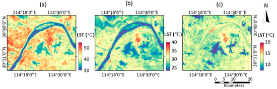
Figure 3.
The spatial distributions of the land surface temperatures (LSTs): (a) Summer, (b) the transition season and (c) winter.
Table 2.
The statistical summary of the retrieved LSTs for all seasons.
4.2. The Spatial Patterns of the Selected Indicators
FVC, albedo, WP, BD, BH and BVD were selected from the original 10 indicators for further modeling after the multiple multicollinearity test (VIF < 10). Such a combination is sufficient to illustrate the LULC heterogeneity of the study area. Among all six indicators, FVC and albedo demonstrated evident seasonal variations, as statistically summarized in Table 3 and visually shown in Figure 4. The spatial patterns of FVC in summer and the transition season were generally consistent, while that of winter revealed a distinct difference with vegetation decaying. The spatial patterns of albedo were generally consistent among the seasons, however, the overall value keeps decreased from summer to the transition season and then winter. By contrast, WP reveals much less variation (Table 3) as water bodies were generally constant despite a subtle seasonal change in water level. As a result, only the WP of summer was presented in Figure 5a. BD, BH and BVD demonstrated a certain change from summer and the transition season to winter along with urbanization. Nevertheless, such change was too imperceptible (Table 3) that only the spatial distributions of the three indicators in summer were visually displayed, as shown in Figure 5b–d. These three indicators illustrated the heterogeneity of the built environment effectively. Generally, the spatial distribution of BD accorded with the corresponding LST pattern in summer (Figure 3a) the most.
Table 3.
The statistical summary of the selected landscape indicators.
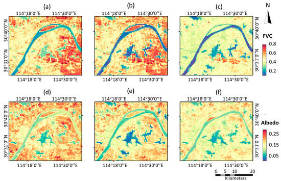
Figure 4.
The spatial distributions of the indicators preserving evident seasonal variations. (a–c) Respectively represent the fractional vegetation cover (FVC) of summer, the transition season and winter; (d–f) albedo.
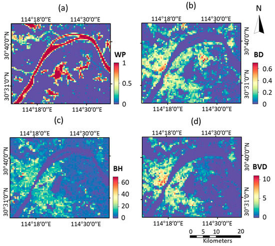
Figure 5.
The spatial distributions of the indicators preserving indistinctive seasonal variations, taking summer as an example. (a) WP, (b) BD, (c) BH and (d) BVD.
4.3. Performace Summary the Three Regression Models
GWR series models were evaluated to be superior to OLS in terms of goodness-of-fit, especially for MGWR, which indicates the assumption of spatially constant unrealistic for exploring the associations between urban landscape and LST. The evaluation summary of the three models, which include R2, AICc and RSS was presented in Table 4. The R2 increased evidently from OLS to GWR for all three seasons, especially for winter from 0.5302 to 0.8681. The R2 of MGWR further exceeded that of GWR although the difference was not significant for summer and the transition season. Besides, the AICc and RSS also decreased remarkably from OLS to GWR and then MGWR, signifying a significant improvement in model fitting.
Table 4.
An evaluation summary of the performance of ordinary least squares (OLS), geographically weighted regression (GWR) and multi-scale geographically weighted regression (MGWR).
The evident difference in the optimal bandwidths identified by MGWR and GWR, as presented in Table 5, highlights the importance of scale in exploring the spatial non-stationary association between LST and different indicators. Based on the results of MGWR, the operating scales for FVC, albedo and BD maintained as a local level despite certain seasonal variations, indicating a significant spatial non-stationarity in the associations with LST for all seasons. The greatest spatial non-stationarity for FVC and albedo presented in winter with the smallest bandwidth, followed by summer and then the transition season. While for BD, the greatest spatial non-stationarity occurred in the transition season, followed by summer and then winter. The association between WP and LST exhibited subtle spatial non-stationarity in summer with a bandwidth of 970, while transfers into global consistence in the transition season and winter with a bandwidth of 4912, which was the number of all pixels involved in the regression. It is interesting to find that BH and BVD interacted with LST in a global manner with a bandwidth of 4912 for all seasons. That is, the impact of BH and BVD on LST was basically consistent across the whole study area.
Table 5.
Optimal bandwidths identified by GWR and MGWR.
4.4. Seasonal Variation of the Non-Stationary Associations
The spatial non-stationary slope coefficients calculated from equation (7), which denotes the contributions of the indicators to LST, were further explored through a boxplot analysis. As shown in Figure 6a, FVC was negatively associated with LST in summer and the transition season with evident spatial non-stationarity. Generally, the cooling effect of vegetation in the transition season was a little bit stronger than that in summer. In contrast, the association in winter was much more complicated with a co-existing negative and positive effect. The impact of albedo on LST (Figure 6b) exhibited a negative or positive effect according to site-specific characteristics for all three seasons. On the whole, the association in winter tended to be much more positive than the other two seasons. WP revealed the most evident negative associations with LST among the six indicators for all seasons (Figure 6c). The cooling effect of water bodies exhibited the best in summer and the transition season. For urban morphology indicators, BD revealed a significant positive association with LST for all three seasons (Figure 6d), especially in the transition season. BH demonstrated the smallest impact on LST among all indicators, as shown in Figure 6e. It is interesting to notice that BH tended to increase LST in summer and the transition season, while decrease in winter. BVD was negatively associated with LST in all seasons with no spatial non-stationarity (Figure 6f). The cooling effect tended to enhance along with the decrease of LST from summer to the transition season and then winter.
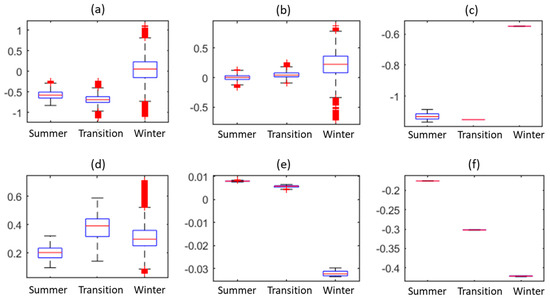
Figure 6.
The boxplots of the slope coefficients of the six indicators for all seasons. (a) FVC, (b) albedo, (c) water percentage (WP), (d) building density (BD), (e) building height (BH) and (f) building volume density (BVD).
Those indicators preserving significant spatial non-stationary associations with LST, including FVC, albedo and BD, were further explored in terms of slope coefficient as visually presented in Figure 7. It is noteworthy that the coefficients generated by MGWR were displayed as smoothing surfaces. Specifically, the slope coefficients of FVC (Figure 7a–c) in all seasons demonstrated a generally consistent spatial pattern in the non-water body area despite the significant value difference for winter. However, it is noticeable that the negative effect of vegetation in the Qingshan industrial district was evidently the strongest across the whole study area in the transition season and winter, which was different from summer. For albedo (Figure 7d–f), the spatial patterns for summer and the transition season were similar. Nevertheless, the level of spatial non-stationarity in winter was significantly higher than summer and the transition season, as the bandwidth for the winter regression was much smaller (Table 5). The strongest cooling effect of albedo in the transition season and winter was also observed in the Qingshan industrial district, especially for winter. The spatial patterns of BD in summer and the transition season were also basically consistent except for the relative stronger heating effect in the transition season, as shown in Figure 7g–i. In contrast, the spatial non-stationarity level for winter was much smaller. Besides, the slope coefficient for winter demonstrated a totally different pattern with an abnormal large level of value in the Qingshan industrial district and surroundings. On the whole, all indicators exhibited certain spatial non-stationarity for their contributions to LST in the built up area for all seasons, thus calling upon site-specific mitigation for localized UHI problems.
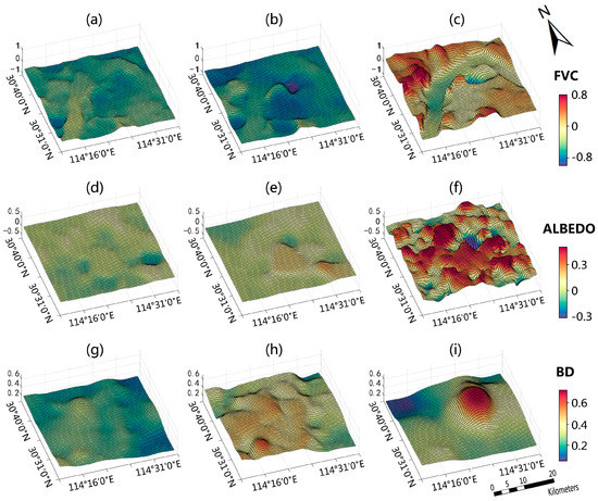
Figure 7.
The spatial non-stationary slope coefficients of the indicators. (a–c) Slope coefficients of FVC in summer, the transition season and winter, respectively; (d–f) albedo; and (g–i) BD.
5. Discussion
This study investigated the spatial non-stationary associations between landscape indicators and LST through MGWR, and analyzed the corresponding seasonal variations. Compared to previous studies, which either utilized local regression models for static LST mechanism exploration [36,38,39,40], or focused on seasonal analysis through global models [14,21,24], this study explored the time-dependent and geographically non-stationary nature of LST mechanism simultaneously. A discussion of the results, application and limitation of this study is presented in the following.
5.1. The Local Landscape Influence and Its Seasonal Variation
The local LST response to urban landscape was observed to possess great seasonal variability, therefore, it is crucial for temperature mitigation and climate modeling to take such seasonal effects into consideration. Generally, such seasonal effect is generated through the seasonal variation of solar thermal radiation and landscape biogeophysical properties [14,21]. Specifically for landscape composition-LST association, consistent with previous studies [14], the presented research revealed that the vegetation index impacted LST the strongest in the transition season, followed by summer and then winter (Figure 6a, Figure 7a–c). The negative effect of vegetation in summer while positive in winter, as indicated by Chun and Guildmann [21], was detected in part of the study area in this research. Such variation is partly contributed by the decrease of photosynthesis in winter [61]. The negative or positive effect in winter depends on the nature of the vegetation [21]. For example, evergreen trees are able to provide winter benefits with sufficient foliage to reduce exposure to cold air and wind, while deciduous trees are incompetent to do so. In consequence, it is significant for landscape designers to consider such seasonal effects so that a year-long effectiveness of greening and land-use policy can be possibly achieved. For LST-albedo association, a positive influence is observed in part of the study area for all seasons, especially in winter (Figure 6b, Figure 7d–f), which is contrary to the generally accepted cooling effect of albedo [61,62]. Further observation revealed that the heating effect generally occurred in areas with relative higher albedo except for water bodies (Figure 4d–f, Figure 7d–f). It is reasonable as cooling effects are normally expected at places with lower albedo under the absence or near-absence of evaporation [73]. The weakest cooling effect of water bodies in winter was also in accordance with previous studies [21,74]. It is interesting to find that water bodies tended to decrease LST in a global manner, especially for the transition season and winter. The result was consistent even if we replaced WP with MNDWI. The less-differentiated biophysical feature of water bodies may have contributed to such consistent contribution to LST.
Besides, urban morphology is also testified to be strongly associated with LST. BD was found to have a stronger influence on LST than BH for all seasons (Figure 6d–e), thus supporting the standpoint that BD is superior to BH for the LST mechanism and mitigation study [75]. The increase of BD tended to heat the local environment by impeding air ventilation, as in agreement with previous studies [28,76,77]. BH exhibited a heating effect in summer and the transition season, but the opposite in winter. Such seasonal variation is consistent with the result of Guo et al. [75]. It is interesting to find that BVD associated with LST negatively for all seasons. Such a result is consistent with Yin et al., [28] where the function-similar floor area ratio (FAR) is utilized in spatial regression without the accompany of SVF. That is, the addition of SVF into the model might reverse the impact of BVD. Among the three morphology indictors used for modeling, only BD demonstrated an evident spatial non-stationarity in the association with LST. In contrast, BH and BVD tended to influence LST in a globally consistent manner in this study. As BD mainly impacts local temperature though air ventilation alteration [28,76,77], the heterogeneous architectural layout, which results in different air ventilation conditions may have partly contributed to the non-stationarity.
5.2. Integration with Planning Practice
This study facilitates the knowledge of environmental implications and planning practices by exploring the season-dependent LST mechanism at an intra-city scale through local regression, hence spatial non-stationarity was highlighted to promote the practicality of city resilience and sustainability. It is broadly proposed to adapt to climate change at the city scale [43,48,78]. Nevertheless, the current city planning regime is still not competent to address the challenges posed by local, regional and global warming [48]. To initiatively bridge with urban planning from thermal environment research through research scale and methodology innovation is thus of great importance for the integration between environmental study and planning practice. The majority of previous works is inclined to use global analysis tools, thus limiting planning practices as cities are treated holistically and intra-city heterogeneity is inevitably ignored. The recent increased propensity of exploring spatial non-stationarity using GWR series models facilitates the translation from environmental knowledge into practical planning applications. The introduction of MGWR further highlights the scale-dependent nature of the spatial non-stationarity by allowing each process to operate under its own intuitive spatial scale. The locally detailed differentiation of the LST mechanism is able to provide sufficient guiding towards site-specific mitigation from urban design and planning [36,40]. In the future, more detailed indicators regarding greenery and BD, such as the size and shape of greenery, and the architectural layout in blocks, can be employed to uncover the underlying mechanism of the spatial non-stationary association with LST, so as to provide detailed guiding for block design.
The locally detailed differentiation of the LST mechanism and the corresponding seasonal variability can also be utilized to optimize the local climate zone (LCZ) approach. LCZ [79] is a newly proposed land surface classification system to divide urban areas into uniform regions with homogeneous temperature behaviors, based on urban morphology, thermal and anthropogenic properties [48]. It is with special significance as it utilizes the zoning custom of urban planning to facilitate the incorporation between the environmental system and city management. However, due to the complexity of urban climatology, LCZ mapping can lead to inconsistencies with LST performance, for example exhibiting only an accuracy of 30.3% in built-up areas of Shanghai [80]. As testified in this study, all six landscape indicators exhibited seasonal variability, and three of them possessed evident spatial non-stationarity regarding the associations with LST. It is thus beyond doubt that a conventional LCZ mapping can result in low accuracy where seasonal variability and spatial non-stationarity are non-negligible. In the future, to improve the accuracy of season-specific LCZ mapping, a weight allocation manner can be employed according to the space-varying LST contribution of each indicator.
5.3. The Limitations
There are several limitations worthy of further discussion. Firstly, this study failed to include urban function into the analysis due to data deficiency. Urban climate is an integrated product of the complicated interactive of both urban form and urban function with the overlying atmosphere [62]. Hence, it is significant to also cover urban function, such as industrial and anthropogenic heat emission into regression modeling. For the spatial non-stationary slope coefficients of FVC (Figure 7c), albedo (Figure 7f) and BD (Figure 7i) in winter, the Qingshan industrial district exhibited abnormal values compared with other areas, which may be attributed to the absence of urban function indicators in the regression. Secondly, the seasonal pattern explored in this study was not complete due to the absence of spring, as the images in spring were all contaminated by cloud. In fact, the common cloud contamination has always impeded the spatio-temporal exploration of urban thermal environment despite the constant sampling frequency of the satellite sensors [10,12,81,82]. As a result, the patterns and dynamics of LST are supposed to partly depend on the LST data available [12,83]. In the future, more efforts can be allocated to the reconstruction of consistent LST data. Thirdly, the seasonal variability and spatial non-stationarity explored in this study might only apply to the block scale. The scale induced difference, especially compared with the canyon scale (30 × 200 m) and neighborhood scale (2 × 2 km) was not considered in this study. Besides, the employment of the un-masked water bodies for complete multivariate regression analysis was also a limitation worthy of improvement in the future.
6. Conclusions
In this study, a state-of-the-art geospatial technique, MGWR, was introduced to investigate the seasonal variations of the spatial non-stationary associations between LST and urban landscape indicators. Based on the localized regression coefficients in different seasons, season- and site-specific strategies towards local temperature problems could be formulated to meet the existing sustainable development goals. The main findings could be summarized as follows: (1) The associations between LST and all six indicators exhibited evident seasonal variations, especially from the transition season to winter. (2) Great spatial non-stationarity was observed in the LST associations with FVC, albedo and BD for all seasons, while WP, BH and BD tended to influence LST in a globally consistent manner. (3) For landscape composition, vegetation exerted a negative effect in summer and the transition season, while a partly positive effect in winter contributed by the nature of greenery. Water bodies exhibited the greatest negative effect among the six indicators for all seasons, although the effects tended to be relatively the weakest in winter. Inconsistent with the generally accepted positive influence, albedo tended to influence LST in a more complicated manner. (4) For urban morphology, BD, with a consistent heating effect on LST, was found to have a stronger influence on LST than BH for all seasons. BH exhibited a positive effect in summer and the transition season, but the opposite in winter. BVD associated with LST negatively for all seasons. The locally detailed differentiation of the LST mechanism for different seasons could further effectively assist the formulation of season- and site-specific mitigation from urban design and planning. Generally, this study facilitates our understanding of human-environment interactions by leveraging the power of geospatial techniques and remote sensing for urban climatology mechanism investigation. However, the absence of urban function indicators and spring LST data due to data deficiency has respectively resulted in abnormal coefficient performance in winter, and the incompleteness of the seasonal patterns. The scale induced difference with other urban climatological scales was also not explicitly explored. In the future, both urban form and urban function will be integrated into modeling. Besides, more detailed indicators regarding vegetation and block structure will be utilized to uncover the underlying mechanism of the spatial non-stationary association with LST, and thus provide detailed guiding for block design.
Author Contributions
H.L. proposed the research concept, designed the experiments, conducted data analysis, and composed the manuscript. Q.Z. designed the framework of this research and participated in manuscript editing. S.G. participated in the data preparation and analysis. C.Y. participated in the data preparation and panel discussion.
Funding
This research is supported by the National Natural Science Foundation of China (No. 51878515, 41331175 and 51378399).
Acknowledgments
We also thank the three anonymous reviewers for their insightful comments that have been very helpful in improving this paper.
Conflicts of Interest
The authors declare no conflict of interest.
References
- Peng, J.; Ma, J.; Liu, Q.; Liu, Y.; Hu, Y.; Li, Y.; Yue, Y. Spatial-Temporal Change of Land Surface Temperature across 285 Cities in China: An Urban-Rural Contrast Perspective. Sci. Total Environ. 2018, 635, 487–497. [Google Scholar] [CrossRef] [PubMed]
- Foley, J.A.; DeFries, R.; Asner, G.P.; Barford, C.; Bonan, G.; Carpenter, S.R.; Chapin, F.S.; Coe, M.T.; Daily, G.C.; Gibbs, H.K.; et al. Global Consequences of Land Use. Science 2005, 309, 570–574. [Google Scholar] [CrossRef]
- Grimm, N.B.; Faeth, S.H.; Golubiewski, N.E.; Redman, C.L.; Wu, J.; Bai, X.; Briggs, J.M.; Grimm, N. Global Change and the Ecology of Cities. Science 2008, 319, 756–760. [Google Scholar] [CrossRef] [PubMed]
- Fu, P.; Weng, Q. A Time Series Analysis of Urbanization Induced Land Use and Land Cover Change and Its Impact on Land Surface Temperature With Landsat Imagery. Remote Sens. Environ. 2016, 175, 205–214. [Google Scholar] [CrossRef]
- Liu, H.; Zhan, Q.; Yang, C.; Wang, J. Characterizing the Spatio-Temporal Pattern of Land Surface Temperature through Time Series Clustering: Based on the Latent Pattern and Morphology. Remote Sens. 2018, 10, 654. [Google Scholar] [CrossRef]
- Huang, S.; Taniguchi, M.; Yamano, M.; Wang, C.-H. Detecting Urbanization Effects on Surface and Subsurface Thermal Environment — A Case Study of Osaka. Sci. Total Environ. 2009, 407, 3142–3152. [Google Scholar] [CrossRef]
- Zhou, D.; Xiao, J.; Bonafoni, S.; Berger, C.; Deilami, K.; Zhou, Y.; Frolking, S.; Yao, R.; Qiao, Z.; Sobrino, J.A. Satellite Remote Sensing of Surface Urban Heat Islands: Progress, Challenges, and Perspectives. Remote Sens. 2019, 11, 48. [Google Scholar] [CrossRef]
- Patz, J.A.; Campbell-Lendrum, D.; Holloway, T.; Foley, J.A. Impact of Regional Climate Change on Human Health. Nat. Cell Boil. 2005, 438, 310–317. [Google Scholar] [CrossRef] [PubMed]
- Weng, Q. Thermal Infrared Remote Sensing for Urban Climate and Environmental Studies: Methods, Applications, and Trends. ISPRS J. Photogramm. Sens. 2009, 64, 335–344. [Google Scholar] [CrossRef]
- Fu, P.; Weng, Q. Temporal Dynamics of Land Surface Temperature From Landsat TIR Time Series Images. IEEE Geosci. Sens. Lett. 2015, 12, 1–5. [Google Scholar] [CrossRef]
- Tran, D.X.; Pla, F.; Latorre-Carmona, P.; Myint, S.W.; Caetano, M.; Kieu, H.V. Characterizing the Relationship Between Land Use Land Cover Change and Land Surface Temperature. ISPRS J. Photogramm. Sens. 2017, 124, 119–132. [Google Scholar] [CrossRef]
- Liu, H.; Zhan, Q.; Yang, C.; Wang, J. The Multi-Timescale Temporal Patterns and Dynamics of Land Surface Temperature Using Ensemble Empirical Mode Decomposition. Sci. Total Environ. 2019, 652, 243–255. [Google Scholar] [CrossRef] [PubMed]
- Kalnay, E.; Cai, M. Impact of Urbanization and Land-Use Change on Climate. Nat. Cell Boil. 2003, 423, 528–531. [Google Scholar] [CrossRef] [PubMed]
- Peng, J.; Jia, J.; Liu, Y.; Li, H.; Wu, J. Seasonal Contrast of the Dominant Factors for Spatial Distribution of Land Surface Temperature in Urban Areas. Remote Sens. Environ. 2018, 215, 255–267. [Google Scholar] [CrossRef]
- Chen, X.-L.; Zhao, H.-M.; Li, P.-X.; Yin, Z.-Y. Remote Sensing Image-Based Analysis of the Relationship Between Urban Heat Island and Land use/Cover Changes. Remote Sens. Environ. 2006, 104, 133–146. [Google Scholar] [CrossRef]
- Du, S.; Xiong, Z.; Wang, Y.; Guo, L. Quantifying the Multilevel Effects of Landscape Composition and configuration on Land Surface Temperature. Remote Sens. Environ. 2016, 178, 84–92. [Google Scholar] [CrossRef]
- Berger, C.; Rosentreter, J.; Voltersen, M.; Baumgart, C.; Schmullius, C.; Hese, S. Spatio-Temporal Analysis of the Relationship Between 2D/3D Urban Site Characteristics and Land Surface Temperature. Remote Sens. Environ. 2017, 193, 225–243. [Google Scholar] [CrossRef]
- Peng, J.; Xie, P.; Liu, Y.; Ma, J. Urban Thermal Environment Dynamics and Associated Landscape Pattern Factors: A Case Study in the Beijing Metropolitan Region. Remote Sens. Environ. 2016, 173, 145–155. [Google Scholar] [CrossRef]
- Liu, Y.; Peng, J.; Wang, Y. Efficiency of Landscape Metrics Characterizing Urban Land Surface Temperature. Landsc. Urban Plan. 2018, 180, 36–53. [Google Scholar] [CrossRef]
- He, B.-J.; Zhao, Z.-Q.; Shen, L.-D.; Wang, H.-B.; Li, L.-G.; He, B.-J. An Approach to Examining Performances of cool/hot Sources in mitigating/Enhancing Land Surface Temperature under Different Temperature Backgrounds Based on Landsat 8 Image. Sustain. Cities Soc. 2019, 44, 416–427. [Google Scholar] [CrossRef]
- Chun, B.; Guldmann, J.-M. Impact of Greening on the Urban Heat Island: Seasonal Variations and Mitigation Strategies. Comput. Environ. Urban Syst. 2018, 71, 165–176. [Google Scholar] [CrossRef]
- Sun, R.; Lü, Y.; Yang, X.; Chen, L. Understanding the Variability of Urban Heat Islands from Local Background Climate and Urbanization. J. Clean. Prod. 2019, 208, 743–752. [Google Scholar] [CrossRef]
- Qiao, Z.; Tian, G.; Xiao, L. Diurnal and Seasonal Impacts of Urbanization on the Urban Thermal Environment: A Case Study of Beijing Using MODIS Data. ISPRS J. Photogramm. Sens. 2013, 85, 93–101. [Google Scholar] [CrossRef]
- Ayanlade, A. Seasonality in the Daytime and Night-Time Intensity of Land Surface Temperature in a Tropical City Area. Sci. Total. Environ. 2016, 557, 415–424. [Google Scholar] [CrossRef] [PubMed]
- Weng, Q.; Lu, D.; Schubring, J. Estimation of Land Surface temperature–vegetation Abundance Relationship for Urban Heat Island Studies. Remote Sens. Environ. 2004, 89, 467–483. [Google Scholar] [CrossRef]
- Song, J.; Du, S.; Feng, X.; Guo, L. The Relationships Between Landscape Compositions and Land Surface Temperature: Quantifying Their Resolution Sensitivity With Spatial Regression Models. Landsc. Urban Plan. 2014, 123, 145–157. [Google Scholar] [CrossRef]
- Wang, J.; Qingming, Z.; Guo, H.; Jin, Z. Characterizing the Spatial Dynamics of Land Surface temperature–impervious Surface Fraction Relationship. Int. J. Appl. Earth Obs. Geoinf. 2016, 45, 55–65. [Google Scholar] [CrossRef]
- Yin, C.; Yuan, M.; Lu, Y.; Huang, Y.; Liu, Y. Effects of Urban Form on the Urban Heat Island Effect Based on Spatial Regression Model. Sci. Total Environ. 2018, 634, 696–704. [Google Scholar] [CrossRef]
- Fotheringham, A.S.; Brunsdon, C.; Charlton, M. Geographically Weighted Regression—The Analysis of Spatially Varying Relationships; John Wiley & Sons Ltd.: West Sussex, UK, 2002. [Google Scholar]
- Goodchild, M.F. The Validity and Usefulness of Laws in Geographic Information Science and Geography. Ann. Assoc. Am. Geogr. 2004, 94, 300–303. [Google Scholar] [CrossRef]
- Anselin, L. Thirty Years of Spatial Econometrics. Pap. Reg. Sci. 2010, 89, 3–25. [Google Scholar] [CrossRef]
- Murakami, D.; Lu, B.; Harris, P.; Brunsdon, C.; Charlton, M.; Nakaya, T.; Griffith, D.A. The Importance of Scale in Spatially Varying Coefficient Modeling. Ann. Am. Assoc. Geogr. 2018, 109, 50–70. [Google Scholar] [CrossRef]
- Foody, G. Geographical Weighting As a Further Refinement to Regression Modelling: An Example Focused on the NDVI–rainfall Relationship. Remote Sens. Environ. 2003, 88, 283–293. [Google Scholar] [CrossRef]
- Wang, Q.; Ni, J.; Tenhunen, J. Application of a Geographically-Weighted Regression Analysis to Estimate Net Primary Production of Chinese Forest Ecosystems. Ecol. Biogeogr. 2005, 14, 379–393. [Google Scholar] [CrossRef]
- Tu, J.; Xia, Z.-G. Examining Spatially Varying Relationships Between Land Use and Water Quality Using Geographically Weighted Regression I: Model Design and Evaluation. Sci. Total Environ. 2008, 407, 358–378. [Google Scholar] [CrossRef]
- Li, C.; Zhao, J.; Xu, Y. Examining Spatiotemporally Varying Effects of Urban Expansion and the Underlying Driving Factors. Sustain. Cities Soc. 2017, 28, 307–320. [Google Scholar] [CrossRef]
- Li, S.; Zhao, Z.; Miaomiao, X.; Wang, Y. Investigating Spatial Non-Stationary and Scale-Dependent Relationships Between Urban Surface Temperature and Environmental Factors Using Geographically Weighted Regression. Environ. Model. Softw. 2010, 25, 1789–1800. [Google Scholar] [CrossRef]
- Su, Y.-F.; Foody, G.M.; Cheng, K.-S. Spatial Non-Stationarity in the Relationships Between Land Cover and Surface Temperature in an Urban Heat Island and Its Impacts on Thermally Sensitive Populations. Landsc. Urban Plan. 2012, 107, 172–180. [Google Scholar] [CrossRef]
- Sun, R.; Xie, W.; Chen, L. A Landscape Connectivity Model to Quantify Contributions of Heat Sources and Sinks in Urban Regions. Landsc. Urban Plan. 2018, 178, 43–50. [Google Scholar] [CrossRef]
- Zhao, C.; Jensen, J.; Weng, Q.; Weaver, R. A Geographically Weighted Regression Analysis of the Underlying Factors Related to the Surface Urban Heat Island Phenomenon. Remote Sens. 2018, 10, 1428. [Google Scholar] [CrossRef]
- Tobler, W.R. A Computer Movie Simulating Urban Growth in the Detroit Region. Econ. Geogr. 1970, 46, 234. [Google Scholar] [CrossRef]
- Fotheringham, A.S.; Yang, W.; Kang, W. Multiscale Geographically Weighted Regression (MGWR). Ann. Am. Assoc. Geogr. 2017, 107, 1247–1265. [Google Scholar] [CrossRef]
- Georgescu, M.; Morefield, P.E.; Bierwagen, B.G.; Weaver, C.P. Urban Adaptation Can Roll Back Warming of Emerging Megapolitan Regions. Proc. Acad. Sci. 2014, 111, 2909–2914. [Google Scholar] [CrossRef]
- Levin, S.A. The Problem of Pattern and Scale in Ecology. Ecol. Time Ser. 1992, 73, 277–326. [Google Scholar] [CrossRef]
- Sayre, N.F. A Companion to Environmental Geography; Wiley Online Library: Hoboken, NJ, USA, 2009. [Google Scholar] [CrossRef]
- Goodchild, M. Models of Scale and Scales of Modelling. In Modelling Scale in Geographic Information Science; Tate, N., Atkinson, P.M., Eds.; Wiley: Chichester, UK, 2001; pp. 3–10. [Google Scholar]
- McMaster, R.B.; Sheppard, E. Introduction: Scale and Geographic Inquiry. In Scale and Geographic Inquiry: Nature, Society and Method; Sheppard, E., McMaster, R.B., Eds.; Blackwell Publishing Ltd.: Malden, MA, USA, 2004. [Google Scholar] [CrossRef]
- Perera, N.; Emmanuel, R.; Perera, N. A “Local Climate Zone” Based Approach to Urban Planning in Colombo, Sri Lanka. Urban Clim. 2018, 23, 188–203. [Google Scholar] [CrossRef]
- Xu, Y.; Ren, C.; Ma, P.; Ho, J.; Wang, W.; Lau, K.K.-L.; Lin, H.; Ng, E. Urban Morphology Detection and Computation for Urban Climate Research. Landsc. Urban Plan. 2017, 167, 212–224. [Google Scholar] [CrossRef]
- He, B.; Ding, L.; Prasad, D. Enhancing Urban Ventilation Performance through the Development of Precinct Ventilation Zones: A Case Study Based on the Greater Sydney, Australia. Sustain. Cities Soc. 2019, 47, 101472. [Google Scholar] [CrossRef]
- Cai, Z.; Han, G.; Chen, M. Do Water Bodies Play an Important Role in the Relationship Between Urban Form and Land Surface Temperature? Sustain. Cities Soc. 2018, 39, 487–498. [Google Scholar] [CrossRef]
- Zhou, W.; Huang, G.; Cadenasso, M.L. Does Spatial Configuration Matter? Understanding the Effects of Land Cover Pattern on Land Surface Temperature in Urban Landscapes. Landsc. Urban Plan. 2011, 102, 54–63. [Google Scholar] [CrossRef]
- Guo, G.; Wu, Z.; Xiao, R.; Chen, Y.; Liu, X.; Zhang, X. Impacts of Urban Biophysical Composition on Land Surface Temperature in Urban Heat Island Clusters. Landsc. Urban Plan. 2015, 135, 1–10. [Google Scholar] [CrossRef]
- Zhou, X.; Chen, H. Impact of Urbanization-Related Land Use Land Cover Changes and Urban Morphology Changes on the Urban Heat Island Phenomenon. Sci. Total Environ. 2018, 635, 1467–1476. [Google Scholar] [CrossRef]
- Lam, J.C.; Tsang, C.; Li, D.H. Long Term Ambient Temperature Analysis and Energy Use Implications in Hong Kong. Energy Convers. Manag. 2004, 45, 315–327. [Google Scholar] [CrossRef]
- Sobrino, J.A.; Jiménez-Muñoz, J.C.; Paolini, L. Land Surface Temperature Retrieval from LANDSAT TM 5. Remote Sens. Environ. 2004, 90, 434–440. [Google Scholar] [CrossRef]
- Yu, X.; Guo, X.; Wu, Z. Land Surface Temperature Retrieval from Landsat 8 TIRS—Comparison Between Radiative Transfer Equation-Based Method, Split Window Algorithm and Single Channel Method. Remote Sens. 2014, 6, 9829–9852. [Google Scholar] [CrossRef]
- Barsi, J.A.; Schott, J.R.; Palluconi, F.D.; Helder, D.L.; Hook, S.J.; Markham, B.L.; Chander, G. Landsat TM and ETM+ Thermal Band Calibration. Can. J. Remote Sens. 2003, 29, 141–153. [Google Scholar] [CrossRef]
- Agam, N.; Kustas, W.P.; Anderson, M.C.; Li, F.; Neale, C.M. A Vegetation Index Based Technique for Spatial Sharpening of Thermal Imagery. Remote Sens. Environ. 2007, 107, 545–558. [Google Scholar] [CrossRef]
- Eswar, R.; Sekhar, M.; Bhattacharya, B.K. Disaggregation of LST over India: Comparative Analysis of Different Vegetation Indices. Int. J. Sens. 2016, 37, 1035–1054. [Google Scholar] [CrossRef]
- Haashemi, S.; Weng, Q.; Darvishi, A.; Alavipanah, S.K. Seasonal Variations of the Surface Urban Heat Island in a Semi-Arid City. Remote Sens. 2016, 8, 352. [Google Scholar] [CrossRef]
- Bonafoni, S.; Baldinelli, G.; Rotili, A.; Verducci, P. Albedo and Surface Temperature Relation in Urban Areas: Analysis With Different Sensors. In Proceedings of the Urban Remote Sensing Event (JURSE 2017), Dubai, UAE, 6–8 March 2017. [Google Scholar]
- Fox, J. Applied Regression Analysis and Generalized Linear Models. Available online: https://socialsciences.mcmaster.ca/jfox/Books/Applied-Regression-2E/JASA-review.pdf (accessed on 18 March 2019).
- Shoff, C.; Yang, T.-C. Spatially Varying Predictors of Teenage Birth Rates Among Counties in the United States. Demogr. Res. 2012, 27, 377–418. [Google Scholar] [CrossRef]
- Shaker, R.R. The Well-Being of Nations: An Empirical Assessment of Sustainable Urbanization for Europe. Int. J. Sustain. Dev. World Ecol. 2015, 22, 1–13. [Google Scholar] [CrossRef]
- Gholizadeh, H.; Robeson, S.M. Revisiting Empirical Ocean-Colour Algorithms for Remote Estimation of Chlorophyll- a Content on a Global Scale. Int. J. Sens. 2016, 37, 2682–2705. [Google Scholar] [CrossRef]
- Ridd, M.K. Exploring a V-I-S (vegetation-Impervious Surface-Soil) Model for Urban Ecosystem Analysis through Remote Sensing: Comparative Anatomy for cities†. Int. J. Sens. 1995, 16, 2165–2185. [Google Scholar] [CrossRef]
- Liang, S. Narrowband to Broadband Conversions of Land Surface Albedo I. Remote Sens. Environ. 2001, 76, 213–238. [Google Scholar] [CrossRef]
- Gál, T.; Unger, J. A New Software Tool for SVF Calculations Using Building and Tree-Crown Databases. Urban Clim. 2014, 10, 594–606. [Google Scholar] [CrossRef]
- Oke, T.R.; Mills, G.; Christen, A.; Voogt, J.A. Urban Climates; Cambridge University Press: Cambridge, UK, 2017. [Google Scholar]
- Wang, Y.; Zhan, Q.; Ouyang, W. Impact of Urban Climate Landscape Patterns on Land Surface Temperature in Wuhan, China. Sustainability 2017, 9, 1700. [Google Scholar] [CrossRef]
- Sobrino, J.A.; Oltra-Carrió, R.; Soria, G.; Bianchi, R.; Paganini, M. Impact of Spatial Resolution and Satellite Overpass Time on Evaluation of the Surface Urban Heat Island Effects. Remote Sens. Environ. 2012, 117, 50–56. [Google Scholar] [CrossRef]
- Ahrends, H.E.; Oberbauer, S.F.; Eugster, W. Small-Scale Albedo-Temperature Relationship Contrast With Large-Scale Relations in Alaskan Acidic Tussock Tundra. In Proceedings of the SPIE 8531, Remote Sensing for Agriculture, Ecosystems, and Hydrology XIV, 8531, Edinburgh, UK, 5 November 2012. [Google Scholar] [CrossRef]
- Huang, Q.; Huang, J.; Yang, X.; Fang, C.; Liang, Y. Quantifying the Seasonal Contribution of Coupling Urban Land Use Types on Urban Heat Island Using Land Contribution Index: A Case Study in Wuhan, China. Sustain. Cities Soc. 2019, 44, 666–675. [Google Scholar] [CrossRef]
- Guo, G.; Zhou, X.; Wu, Z.; Xiao, R.; Chen, Y. Characterizing the Impact of Urban Morphology Heterogeneity on Land Surface Temperature in Guangzhou, China. Environ. Model. Softw. 2016, 84, 427–439. [Google Scholar] [CrossRef]
- Yang, J.; Su, J.; Xia, J.C.; Jin, C.; Li, X.; Ge, Q. The Impact of Spatial Form of Urban Architecture on the Urban Thermal Environment: A Case Study of the Zhongshan District, Dalian, China. IEEE J. Sel. Top. Appl. Earth Obs. Sens. 2018, 11, 2709–2716. [Google Scholar] [CrossRef]
- Yang, J.; Jin, S.; Xiao, X.; Jin, C.; Xia, J.C.; Li, X.; Wang, S. Local Climate Zone Ventilation and Urban Land Surface Temperatures: Towards a Performance-Based and Wind-Sensitive Planning Proposal in Megacities. Sustain. Cities Soc. 2019, 47, 101487. [Google Scholar] [CrossRef]
- Seto, K.C.; Golden, J.S.; Alberti, M.; Turner, B.L. Sustainability in an Urbanizing Planet. Proc. Acad. Sci. 2017, 114, 8935–8938. [Google Scholar] [CrossRef]
- Stewart, I.D.; Oke, T.R. Local Climate Zones for Urban Temperature Studies. Am. Meteorol. Soc. 2012, 93, 1879–1900. [Google Scholar] [CrossRef]
- Cai, M.; Ren, C.; Xu, Y.; Lau, K.K.; Wang, R. Investigating the Relationship Between Local Climate Zone and Land Surface Temperature Using an Improved WUDAPT Methodology—A Case Study of Yangtze River Delta, China. Urban Clim. 2018, 24, 485–502. [Google Scholar] [CrossRef]
- Pede, T.; Mountrakis, G. An Empirical Comparison of Interpolation Methods for MODIS 8-Day Land Surface Temperature Composites across the Conterminous Unites States. ISPRS J. Photogramm. Sens. 2018, 142, 137–150. [Google Scholar] [CrossRef]
- Zou, Z.; Zhan, W.; Liu, Z.; Bechtel, B.; Gao, L.; Hong, F.; Huang, F.; Lai, J. Enhanced Modeling of Annual Temperature Cycles With Temporally Discrete Remotely Sensed Thermal Observations. Remote Sens. 2018, 10, 650. [Google Scholar] [CrossRef]
- Bechtel, B.; Sismanidis, P. Time Series Analysis of Moderate Resolution Land Surface Temperatures. In Remote Sensing: Time Series Image Processing; Weng, Q., Ed.; Taylor & Francis: Abingdon, UK, 2017. [Google Scholar]


© 2019 by the authors. Licensee MDPI, Basel, Switzerland. This article is an open access article distributed under the terms and conditions of the Creative Commons Attribution (CC BY) license (http://creativecommons.org/licenses/by/4.0/).