Abstract
As an indispensable ecological parameter, surface soil moisture (SSM) is of great significance for understanding the growth status of vegetation. The cooperative use of synthetic aperture radar (SAR) and optical data has the advantage of considering both vegetation and underlying soil scattering information, which is suitable for SSM monitoring of vegetation areas. The main purpose of this paper is to establish an inversion approach using Terra-SAR and Landsat-7 data to estimate SSM at three different stages of corn growth in the irrigated area. A combined scattering model that can adequately represent the scattering characteristics of the vegetation coverage area is proposed by modifying the water cloud model (WCM) to reduce the effect of vegetation on the total SAR backscattering. The backscattering from the underlying soil is expressed by an empirical model with good performance in X-band. The modified water cloud model (MWCM) as a function of normalized differential vegetation index (NDVI) considers the contribution of vegetation to the backscattering signal. An inversion technique based on artificial neural network (ANN) is used to invert the combined scattering model for SSM estimation. The inversion method is established and verified using datasets of three different growth stages of corn. Using the proposed method, we estimate the SSM with a correlation coefficient and root-mean-square error 0.043 cm/cm at the emergence stage, with and 0.046 cm/cm at the trefoil stage and with and 0.064 cm/cm at the jointing stage. The results suggest that the method proposed in this paper has operational potential in estimating SSM from Terra-SAR and Landsat-7 data at different stages of early corn growth.
1. Introduction
Although surface soil moisture (SSM) accounts for only a small part of the entire water cycle, it is a crucial basis for various hydrological, biological, and biogeochemical processes. It controls the distribution between surface infiltration and surface runoff, and is a primary factor for energy exchange between land and atmosphere [1]. In agricultural production, the accurate acquisition of SSM with high temporal and spatial resolution is particularly important for precision irrigation, crop growth monitoring and field estimation [2]. However, the measurement of SSM by in-situ sensors is not only costly, but also cannot effectively capture the spatiotemporal variability of SSM, especially in large irrigation areas [3,4,5]. In addition, unlike atmospheric pressure and other meteorological variables, SSM has the characteristics of high inhomogeneity and large spatial variation, so it is difficult to obtain the accuracy that meets the requirements of precision irrigation and field estimation [6]. Satellite remote sensing observations have considerable potential to describe SSM at different scales in a consistent, timely, and cost-effective manner [7,8,9,10,11,12]. Optical remote sensing data is mainly used to estimate crop vegetation parameters in agricultural applications [13]. There are also some studies that use thermal infrared data to measure surface temperature and estimate SSM [14,15,16]. Compared with optical remote sensing, the application of microwave remote sensing technology in SSM acquisition has attracted much attention due to its high sensitivity to soil dielectric constant and flexible all-weather and full-time sensing capabilities [17,18,19,20]. As a kind of active microwave remote sensing with high spatial resolution and high penetrating ability, synthetic aperture radar (SAR) has been widely studied in the restoration of SSM [21,22,23,24,25,26,27,28,29].
Several studies have proven that there is a strong correlation between radar backscattering coefficients and SSM on bare surface and sparse vegetation areas [23,27,28,30]. Therefore, various scholars have established models to estimate SSM. These models can be roughly divided into three categories [21]. The first type is the theoretical model, such as small perturbation model [31], integral equation model (IEM) [32], and Kirchhoff model (KM) [33]. These models are based on radiative transfer equations and can describe the relationship between SSM and SAR backscattering coefficients in different geographical areas. However, the theoretical model expressions are complex and require many field measurements, so there are a multitude of limitations in practical applications. The second type is the semi-empirical model combining empirical and theoretical models [34,35]. The last type is the empirical model represented by the regression model [36], Oh model [37], and Dubois model [38,39]. The experimental relationship between SSM and SAR backscattering coefficients is based on measured data and actual scenarios. Empirical models can perform well under the conditions corresponding to the scenario where the actual data is measured. In addition, due to the concise expression of the empirical model, it is used by many scholars to invert the SSM [36,37,38,39].
For farmland areas covered by vegetation, the SAR backscattering coefficient is related to vegetation coverage in addition to surface scattering. If the aforementioned model is used to invert the SSM of the surface under vegetation, it will cause an underestimation of the SSM [21,40]. In order to obtain accurate SSM estimates, it is necessary to combine the vegetation scattering model. Common vegetation scattering models include the Michigan microwave canopy scattering model (MIMICS) [41] and the water cloud model (WCM) [42]. The MIMICS model is a complex vegetation scattering model, which requires many measured parameters. It mainly describes the scattering relationship between vegetation and the earth surface in the forest areas [43]. In contrast, the WCM has been widely studied in the SSM estimation of vegetation areas in the past two decades because of its simple expression and easy-to-obtain vegetation parameters. Most of these studies have used the WCM for SSM estimation from C and X-band SAR and achieved accuracies better than 0.08 cm/cm [23,27,44,45]. In addition, the vegetation parameters required by the WCM can be obtained directly from optical remote sensing, so the collaborative inversion of SSM by optics and SAR has obvious advantages.
With the increase of the amount of SAR data, change detection method [46,47] and artificial neural network (ANN) [23,27,29,48,49] have appeared successively. However, the change detection methods are widely based on the assumption that vegetation changes slowly in the time dimension, and little consideration is given to the effects of vegetation growth [46,50]. In recent years, the ANN method has been extensively studied in estimating SSM [5,51]. El Hajj et al. [23,27] used ANN combined with WCM to estimate SSM for X, C and L band data, respectively. When the normalized differential vegetation index (NDVI) is less than 0.7, the root-mean-square error (RMSE) of the X-band is 0.036 cm/cm, the C-band is 0.046 cm/cm, and the L-band is 0.053 cm/cm. When the NDVI is greater than 0.7, the RMSE is less than 0.08 cm/cm. This shows that under the condition of different thickness of vegetation cover, ANN combined with WCM can accurately estimate the SSM.
Although the above studies have obtained high-precision SSM estimates on both bare ground and vegetation coverage areas, few studies have considered SSM estimates at different stages of vegetation growth. However, the SSM of each growth stage of crops is exactly a exceedingly crucial parameter in agricultural irrigation [52]. At different stages of crop growth, crops vary greatly in shape, height, and coverage [52], especially for altherbosa such as corn, which has large spacing between plants and relatively thick stems.
In this paper, we provide a combined scattering model based on a modified water cloud model (MWCM) (see Section 3.1 and Equations (10) and (11)) and an empirical model proposed by El Hajj et al. [27] to determine the relationship between SSM and SAR backscattering coefficient. The proposed combined scattering model is parameterized by Terra-SAR data, Landsat-7 data and measured SSM data collected from three times from the emergence stage to the jointing stage of corn. In order to prove the effectiveness of the combined scattering model, the performance of simulated SAR backscattering coefficients in three stages of corn growth is compared using WCM and MWCM combined with GOM and the empirical model respectively. Subsequently, a large number of SSM, NDVI and corresponding SAR backscattering coefficient are simulated using the parameterized combined scattering model as the training set of ANN. The trained ANN is used to estimate the SSM on the measured data of corn at three different growth stages. Finally, the estimated SSM is compared with the actual measured SSM to evaluate the accuracy of the model.
The remainder of this paper is organized as follows. Section 2 describes the details of the study area, Terra-SAR data, Landsat-7 data and field measurements. Section 3 introduces the specific content of the combined scattering model and the structure and usage of ANN. The inversion results are presented in Section 4, and the results are discussed in Section 5. Finally, the entire article is summarized in Section 6 and make a prediction for subsequent learning.
2. Study Site and Data Collection
2.1. Study Area
The experimental data in this study is from the Heihe watershed allied telemetry experimental research (HiWATER), which is a multi-scale hydrologic observation experiment conducted in the Heihe river basin (HRB) from 2012 to 2015 [53,54]. The HRB as an experimental watershed is a typical inland river basin located in the arid region of northwestern China. It is located between 97.1–102.0E and 37.7–42.7N, and is associated with alpine and arid areas. Comprehensive observation experiments on snow cover and frozen soil hydrology, irrigation water balance, crop growth, and ecological water consumption are carried out at the upper, middle and lower reaches of the HRB, respectively [54]. In this paper, the data of the farmland irrigated area of the artificial oasis in the middle reaches of the HRB in the HiWATER are selected as the research object. The artificial oasis belongs to temperate arid climate, with an average annual rainfall of 198 mm and an average annual temperature of 7 C. These regions are the largest corn seed production bases in China and have the most comprehensive irrigation infrastructure, mainly river irrigation and well irrigation. Irrigation water quality is good with a pH value of about 8.09, dissolved oxygen of about 8.1 mg/L, permanganate index of about 3.72 mg/L, ammonia nitrogen of about 0.41 mg/L and total phosphorus of about 0.104 mg/L. The experimental region covers an area of 5.5 km × 5.5 km, mainly consisting of villages, roads, orchards, and corn fields, which can represent the crop structure and cultivation method of the middle irrigation area. Figure 1 shows the specific geographic location and surface coverage of the area. The soil texture in the test areas is as follows [55]: clay content: 0.080; sand content: 0.35; loam content: 0.57. The average soil bulk density, saturation moisture capacity and field capacity in the test area are 1.49, 0.39 cm/cm and 0.32 cm/cm respectively [55,56].
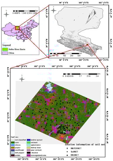
Figure 1.
Study area specific geographical location, land use map and the location of the sensor network.
2.2. In Situ Measurements
The measured SSM data were collected from the sensor network arranged in HiWATER. It provides a multi-scale dataset of meteorological elements and land surface parameters for easy estimation of soil moisture on land surfaces. In this paper, three sensor network datasets in the middle reaches of the HRB are selected as research objects. All the sensors are located in the artificial oasis farmland in the middle reaches of HRB. The range of surface roughness information is [1.0–2.0] cm for root mean square height h and [12.0–16.0] cm for correlation length l [57]. The first sensor network is BNUNET [58], with three soil temperature probes installed at 4, 10, and 20 cm below the land surface and one soil moisture sensor (SPADE) at 4 cm, with an observation frequency of 10 min, from May 2012 to September 2012 [54,55,59]. The second is WATERNET [60], which includes two Steven Hydra Probe II soil moisture and salinity sensors and two soil temperature probes installed at 4 cm and 10 cm below the land surface, with an observation frequency of 10 min, from June 2012 to September 2012 [54,55,59]. The last is SoilNET [61], which includes four SPADE sensors and four soil temperature probes at depths of 4, 10, 20, and 40 cm and observed at intervals of 10 min, from June 2012 to September 2012 [54,55,59]. The location information of the measurement points in the corn coverage area of these sensor networks is shown in Figure 1. Soil moisture sensors SPADE and Hydra Probe II were verified by a two-point calibration method, with one point measured in the desert sand after air seasoning and the other observed in saturated soil sampled from local farmland. The calibration shows that the instrument errors of the SPADE and Hydra Probe II sensors are 0.032 and 0.011 cm/cm [55,57], respectively. Considering the limited penetrability of the X-band, SSM and temperature data at 4 cm of the topsoil are taken into account. The SSM data and soil temperature data in the three datasets with the same acquisition time as the Terra-SAR images are used as the measured data. The Terra-SAR images used for this experiment were acquired on 24 May, 4 June and 26 June 2012, respectively. Only BNUNET was working on 24 May and 4 June, with a total of 64 measurement points in the corn coverage area, and two measurement points were missing data on 4 June. On 26 June, three sensor networks were in operation, including 59 measurement points on the BNUNET network (data missing from five measurement points), 44 measurement points on the SoilNET network and 40 measurement points on the WATERNAT network. Table 1 provides detailed information on SSM for sensor networks in corn fields.

Table 1.
The Terra-SAR data acquisition time (Date) and minimum (Min), maximum (Max), average (Mean), standard deviation (SD), and Number (N) of SSM measurement points.
From 17 May to 9 September 2012, the canopy height of the experimental area was measured 16 times [53,62]. In each measurement, 5 plots were selected from the experimental area, and 10 measuring points were selected from each plot to measure the canopy height. In this paper, considering the acquisition time of Terra-SAR images, the canopy height data measured on 22 May, 4 June, and 25 June are selected as reference. Table 2 summarizes the maximum, minimum and average values of the canopy height. On May 24, corn was in the emergence stage with fast root growth and slow leaf growth, containing two or three leaves with low chlorophyll content, so the canopy height range was approximately equal to the measurement on 22 May. On 4 June, corn was in the trefoil stage, and in addition to root and leaf growth, stems began to differentiate. Corn was characterized by three to seven leaves with increased chlorophyll content. The range of measured vegetation height was [31, 47] cm. On 26 June, the corn was in the jointing stage. At this stage, the leaves and stalks grew rapidly, and the vegetative growth and reproductive growth proceed simultaneously. The range of corn canopy heights can be approximated to be between 81 cm and 130 cm as measured on 25 June.
Table 2.
The measurement date and Min, Max, Mean of canopy height.
2.3. Satellite Data
2.3.1. Landsat-7 Data
Four cloud-free optical images, acquired on 7 May, 8 June, 24 June and 10 July, 2012, of the study site were obtained from the Landsat-7 satellite. Landsat-7 images have a resolution of 30 m and can be downloaded at (https://search.earthdata.nasa.gov). The Environment for Visualizing Images (ENVI) software of Exelis Visual Information Solutions is used to preprocess the Landsat-7 data, including: radiation correction and atmospheric correction. The 3 and 4 bands of Landsat-7 represent the Red (RED) and Near-Infrared (NIR) reflectances, respectively, which are used to calculate the NDVI. The expression is as follows:
The NDVI information corresponding to the measurement points of the sensor network in Section 2.2 is shown in the boxplot of Figure 2. The NDVI maps for four days are shown in Figure 3. It can be concluded from Figure 2 and Figure 3 that NDVI changed significantly between 7 May and 10 July, when corn was in the period from emergence stage to jointing stage, during which corn grew rapidly. If the NDVI obtained by Landsat-7 is directly used, due to the time difference between the SAR and the optical image, there will be SSM estimation errors caused by inaccurate vegetation parameters. Therefore, at each SSM measurement point, the corresponding NDVI value is estimated using a linear interpolation of the two NDVI values calculated from optical images with acquisition dates preceding and succeeding the SAR image [63].
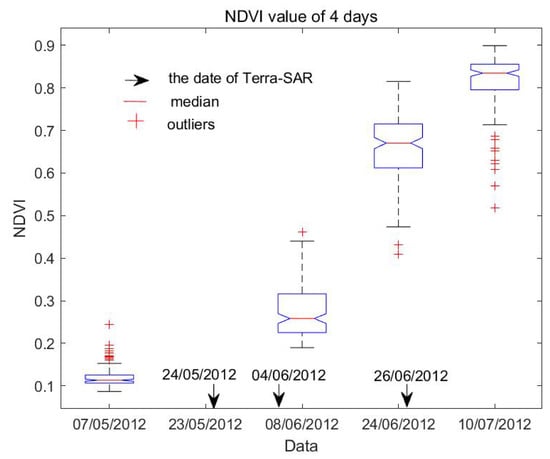
Figure 2.
Boxplot of NDVI values obtained from four Landsat-7 images during the period from emergence stage to jointing stage.
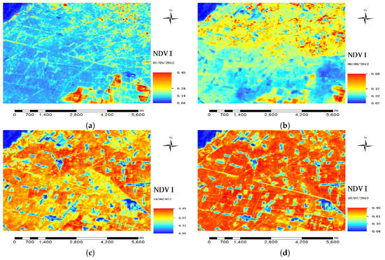
Figure 3.
The NDVI maps for four days. (a) NDVI map on 7 May; (b) NDVI map on 8 June; (c) NDVI map on 24 June; (d) NDVI map on on 10 July.
2.3.2. Terra-SAR Data
From May to August 2012, eight TerraSAR-X images were obtained from the HiWATER, covering the middle reaches of the artificial oasis ecological hydrological experimental area. However, due to the limited ability of the X-band to penetrate vegetation, this paper only takes the first three images as the research object. The three images were acquired on 24 May, 4 June, and 26 June, 2012, corresponding to the emergence, trefoil and jointing stages of corn growth, respectively. The three images obtained are all in StripMap mode, with a nominal resolution of 3 m, and the product level is multi-look ground range detected (MGD). Moreover, the images are in dual-polarization mode (HH and VV) with small incidence angle between 22 and 24 [53]. All Terra-SAR images and in-situ network observations can be obtained at the Cold and Arid Regions Science Data Center (http://westdc.westgis.ac.cn/) [54].
The pre-processing of Terra-SAR images is implemented by the Sentinel Application Platform (SNAP) toolbox provided by the European Space Agency (ESA). The first step is to convert the pixel values of the Terra-SAR image into backscattering coefficient values. For Terra-SAR MGD products, the algorithm developed by the German Aerospace Center (DLR) and the Italian Space Agency (ASI) is used for radiation correction [64]. The expression of the algorithm is:
where is the backscattering coefficient, Ks is the calibration constant provided in the image data, DN is the amplitude of the backscattered signal, is the the radar incidence angle, NESZ is the noise equivalent sigma zero. Subsequently, topographic correction and orthodontic correction are used to correct geometric distortions. In order to reduce noise, a refined Lee filter with a window size of pixels is applied to the Terra-SAR images. To be consistent with Landsat-7, geolocation is performed according to the UTM projection system, with the Landsat-7 image as a reference [65].
In order to ensure that the SAR backscattering coefficient is sensitive to SSM in the three stages of corn growth, the sensitivity analysis of three groups of SSM and backscattering coefficient is performed here. Figure 4 shows the change of HH and VV backscattering coefficients with SSM in three stages of corn growth. The linear regression shown in Figure 4 suggests that the sensitivity of HH and VV to SSM for the three growth stages of corn has a slope (dB/(cm/cm)), which lies between 10 and 20. This sensitivity is not high for the X-band. Anguela et al. [66] found a sensitivity of 35 dB/(cm/cm) between the X-band backscattering coefficient of the bare surface and the SSM with a soil depth of 0–5 cm at an incidence angle of 25 cm/cm. M. Aubert et al. [4] also obtained approximate sensitivity. The low sensitivity in this experiment mainly comes from two reasons. One is that the SSM in this paper is acquired by a sensor fixed at a depth of 4 cm, which cannot represent the average SSM of 0–5 cm. Due to the weak penetration of the X-band, the sensitivity at 4 cm is lower than that at 0–5 cm. Another reason is the presence of vegetative cover in the test area, which can weaken the sensitivity between the backscattering coefficient and SSM. El Hajj et al. [27] also obtained a lower sensitivity of 17 dB/(cm/cm) at X-band in the vegetation covered area. Although the sensitivity between the X-band SAR backscattering coefficient and SSM of the vegetation coverage area is reduced to half of the bare surface, the sensitivity of 10–20 dB/(cm/cm) still has the potential to invert SSM in the early stages of corn growth.
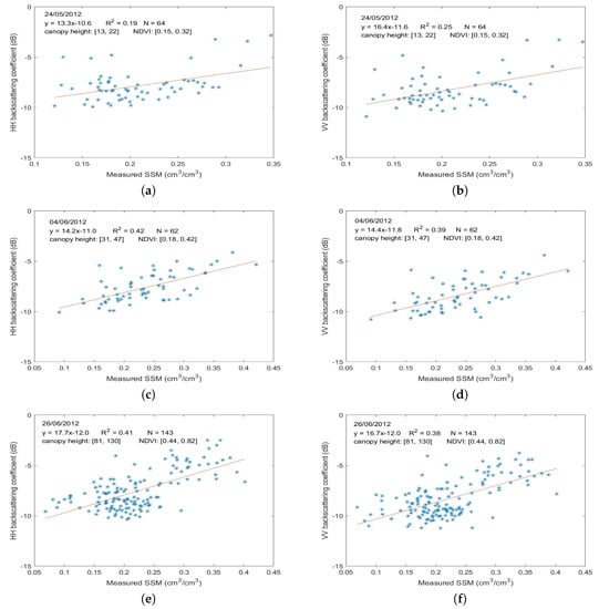
Figure 4.
Backscattering coefficients as a function of SSM for corn cover. (a) Emergence stage, HH polarization; (b) Emergence stage, VV polarization; (c) Trefoil stage, HH polarization; (d) Trefoil stage, VV polarization; (e) Jointing stage, HH polarization; (f) Jointing stage, VV polarization.
3. Method
The proposed algorithm for SSM estimation involves the following four steps:
- Data pre-processing: the SNAP is used to calibrate the Terra-SAR data, converting the digital number of images to backscattering coefficients () in linear units. The Landsat-7 images are converted to NDVI maps using ENVI software.
- Parametric combined scattering model: the dataset consisting of backscattering coefficient, SSM measurement, and NDVI of the three different stages is divided into two sub-datasets. The first sub-dataset (180 calibration sampling points) is used to fit the combined scattering model and the second (89 verification sampling points) is used to validate the model.
- ANN training: a dataset of SAR backscattering coefficient simulated by the parameterized combined scattering model is used to train the ANN.
- SSM retrieval: the trained ANN is applied to the verification sampling points to estimate the SSM, and the potential of the inversion algorithm is evaluated by comparing SSM estimates with measurements.
The overall workflow is shown in Figure 5.
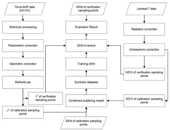
Figure 5.
Overall workflow of the SSM retrieval process.
3.1. Radar Signal Modeling
The most widely used vegetation scattering model is WCM, which assumes that the vegetation layer is uniformly distributed throughout the pixel unit. Therefore, the total backscattering coefficient consists of three dominant components: vegetation canopy scattering , interaction scattering between the underlying soil and vegetation , and underlying soil scattering through two-way attenuation of vegetation layer [67]. The total backscattering coefficient can be expressed as:
where
where A and B are empirical constants to be adjusted later, and are vegetation parameters.
In many studies of vegetation cover areas such as pasture and wheat, the interaction scattering between the underlying soil and vegetation of the WCM is ignored [21,27]. However, when the surface vegetation is covered with altherbosa, the situation is much more complicated. The vegetation in this experimental area is mainly corn, with high plant height, thick stems and large plant spacing. Therefore, the interaction scattering between the underlying soil and vegetation cannot be ignored. Jinyang Du et al. [68] established a theoretical scattering model of vegetation area based on the first-order solution of the radiation transfer equation. Subsequently, the theoretical scattering model was simplified based on leaf-dominated vegetation (e.g., soybean) and stem-dominated vegetation (e.g., corn), respectively. The simplified theoretical scattering model is called first-order physical scattering model. For stem-dominated vegetation, the interaction scattering between the underlying soil and vegetation can be important, which is given in the first-order physical scattering model [67,68]:
where is volume scattering coefficient, d is the thickness of the vegetation layer. During the period of rapid vegetation growth, neither of the two parameters is easy to measure. Therefore, the product of the two parameters is expressed in the form of empirical coefficient C multiplied by a vegetation parameter (). is the surface reflectivity. After comparing the Fresnel reflection coefficient and the polarization amplitude in the experiment, the polarization amplitude is selected to represent this parameter. So the interaction scattering between the underlying soil can be expressed as the following equation:
where C is an empirical constant to be adjusted, the subscript pp in and stands for polarization (HH and VV), and the polarization amplitude is given by:
where is soil relative permittivity, which is expressed by the Dobson model [69]. As an example, for incidence angle of 22, soil temperature of 20 C and SSM of 0.25 cm/cm, the is 11.11 + 3.09i from Dobsol model and the and are −4.8 dB and −3.1 dB, respectively.
In addition, from the corn emergence stage to the jointing stage, there is a long period of time when corn cannot cover the whole pixel unit uniformly, so the MWCM introduces vegetation coverage . In a pixel, the proportion of corn coverage area is , and the proportion of bare surface is . Backscattering of corn coverage area consists of three parts: , and . Backscattering of bare surface is only . Therefore, the total backscattering coefficient is expressed as follows:
Vegetation coverage [52] can be calculated as follows:
The and are the maximum and minimum values of NDVI during the entire measurement process. Various studies have shown that when the vegetation parameters in the WCM is NDVI, it can accurately describe the vegetation scattering characteristics [27], so NDVI is used as the vegetation parameters , , and in this experiment.
3.2. Soil Surface Backscattering
The relationship between SSM and backscattering coefficient can be expressed by an empirical model established by El Hajj et al. [27], which obtained good results in X-band SSM inversion:
where is the backscattering coefficient of underlying soil, D and E are empirical coefficients.
To illustrate the effectiveness of the empirical model, it is compared with a simplified GOM, which also performs well in X-band [70,71,72,73]:
where is the incidence angle, s () is the root-mean-square slope of the surface roughness parameter, h and l are root mean square height and correlation length of the surface roughness (cm), respectively. The Fresnel reflection coefficients at normal incidence are described in a previous study [73]. Since there is no surface roughness information corresponding to the sensor network, an estimated root-mean-square slope is used in this paper. Based on previous research on HiWATER data [57], the h and l of artificial oasis farmland in the middle reaches of HRB are constrained between [1.0, 2.0] cm and [12.0, 16.0] cm, respectively, so the value range of s is constrained to [0.06, 0.17]. The s is increased by 0.01 each time from a minimum value of 0.06 to a maximum value of 0.17. For each s, the experience parameters A, B, and C are calibrated by minimizing the cost function J constructed by RMSE of the simulated backscattering coefficients and the observed backscattering coefficient in HH and VV polarizations:
The root-mean-square slope is considered constant throughout the corn growth cycle due to the plastic film covering. We use the K-fold (K = 10) cross-validation method, which takes the average value s = 0.15 of the K-fold verification results as the root-mean-square slope.
3.3. Surface Soil Moisture Retrieval
In this experiment, SSM is inverted using an ANN trained by the Levenberg-Marquardt algorithm. The ANN consists of 4 layers, one input layer, two hidden layers and one output layer. The output of the ANN is SSM. When using HH or VV polarized backscattering coefficients and NDVI, the input of ANN is a two-dimensional vector. When using HH and VV polarization backscattering coefficients and NDVI, the input of ANN is a three-dimensional vector. The tangent-sigmoidal function and the linear function are used as the activation functions of the hidden layer and the output layer, respectively. By gradually increasing the number of hidden layer neurons, when the first layer of the hidden layer contains 15 neurons and the second layer contains 10 neurons, it provides an accurate estimate of the reference parameters [27].
For the large amount of data required for ANN training, a SAR backscattering coefficient dataset is synthesized using the parameterized Equations (10) and (12), in which the input parameters are SSM, NDVI and incidence Angle. The soil temperature is only used in the Dobson model, which has very little effect on the backscattering coefficient, so it is ignored in dataset synthesis. Simultaneously, the study area is relatively flat and small, the change of incident Angle can be ignored, so it is set as the average incident angle 23. Throughout the whole process, the maximum and minimum values of the measured SSM are 0.4208 cm/cm and 0.068 cm/cm, respectively. Therefore, the variation range of the SSM of the simulated dataset is set as 0.02 cm/cm to 0.42 cm/cm with the step size increasing by 0.02 cm/cm. In order to better simulate the NDVI information of the three stages of corn growth, the maximum, minimum, and average values of the observed NDVI over the three days are statistically calculated. The details are in Table 3. Referring to Table 3, the NDVI variation range of the simulation data set is set to 0.1 to 0.85, and the increment is set to 0.05. To make the synthetic data more realistic, noise corresponding to the actual SAR data is added to the synthesized datasets [23,27]. The uncertain range is between 0.6 and 1 dB for Terra-SAR sensor [27]. Therefore, in order to obtain a statistically significant dataset, we add 30,000 random samplings of Gaussian noise with a mean value of 0 and a standard deviation of 1 dB to each synthesized backscattering coefficient. Finally, the synthetic dataset is divided into three training configurations: (1) backscattering coefficient in HH and NDVI, (2) backscattering coefficient in VV and NDVI, and (3) backscattering coefficient in both HH and VV and NDVI.
Table 3.
The Max, Min, and Mean values of NDVI observations.
3.4. Evaluation Method
The accuracy of the combined scattering model to simulate the backscattering coefficient (or inversion of SSM) is verified by several effective methods. In addition to the frequently-used RMSE, mean absolute error (MAE) and R, the index of agreement (IA) [74] and ratio of prediction to deviation (RPD) [75,76] are used to assess the accuracy of SSM estimates. The absolute difference and the average of the errors between the observed and estimated backscattering coefficients (or SSM) are expressed as MAE and RMSE [52], respectively. R indicates the strength and sign of the correlation relationship between observed and predicted values. RPD indicates the strength of the statistical correlation between observed and predicted values. IA stands for the degree of agreement between the measurements and observations. They are calculated in the following form:
where is the observed backscattering coefficient (or SSM) at location i, and is the predicted backscattering coefficient (or SSM) at location i. and are the averages of observations and predictions, respectively.
4. Results
In this study, Terra-SAR backscattering coefficient observations, measured SSM data, and NDVI are randomly selected to parameterize the combined scattering model to obtain empirical parameters. Two-thirds of the dataset is used as calibration sampling points, and the remaining one-third is used as verification sampling points. To ensure that the data of each stage can be divided into calibration and verification sample points, the data of each stage is first divided into two parts, and then the calibration sample points of all stages are used to parameterize the combined scattering model. The verification sampling points are used to verify the effectiveness of the combined scattering model and evaluate the potential of the SSM retrieval algorithm in this paper. The number of calibration and verification sampling points is listed in Table 4. Table 5 gives the empirical coefficients of the parameterized combined scattering model at different polarizations.
Table 4.
The number of calibration and verification sampling points.
Table 5.
The empirical coefficients of the parameterized combined scattering model at different polarizations.
4.1. Evaluation of Combined Scattering Model
The purpose of this section is to verify the potential of the combined scattering model proposed in this paper to simulate the behavior of SAR signals at three different stages of corn growth. To illustrate the effectiveness of the combined scattering model, the WCM and the MWCM are combined with the GOM and the empirical model established by El Hajj et al. [27] into four combined scattering models for comparison. The four models are WCM and GOM (WC-GOM), MWCM and GOM (MWC-GOM), WCM and the empirical model (WC-EM), MWCM and the empirical model (MWC-EM). The four combined scattering models are parameterized using the same calibration sampling points. SSM and NDVI from the verification sampling points are substituted into the parameterized combined scattering models to calculate the backscattering coefficient.
Figure 6 displays the scatterplots between Terra-SAR and simulated backscattering coefficients using the four combined scattering models for the verification sampling points (with 1:1 blue line shown). In both HH and VV polarizations, the backscattering coefficients simulated by the MWC-EM (red asterisk) are closer to the observed backscattering coefficients than the other three models. When the observed backscattering coefficient is less than −8 dB, the backscattering coefficients simulated by WC-GOM and MWC-GOM are overestimated. When the observed backscattering coefficient is greater than −8 dB, they are underestimated. In contrast, there is no obvious overestimation and underestimation of the backscattering coefficients simulated by WC-EM and MWC-EM. This phenomenon may be due to the fact that the GOM cannot accurately estimate underlying soil scattering.
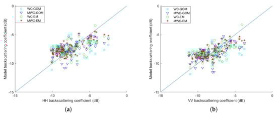
Figure 6.
Comparison of actual SAR backscattering coefficients data with simulations using different models. (a) HH polarization; (b) VV polarization.
Table 6 summarizes the statistics of the SAR backscattering coefficient estimation accuracy of the verification sample points at three different stages and all stages. According to the statistical analysis, the conclusions consistent with Figure 6 can be drawn. Overall, the MAE and RMSE calculated by MWC-EM are the smallest of those four methods, in the range of [0.8, 1.1] dB and [0.9, 1.3] dB, respectively. Except for 24 May (the emergence stage), the R and IA calculated by MWC-EM is higher than the value calculated by the other three models. During the three stages of corn growth, the IA and RPD between the observed backscattering coefficient and the backscattering coefficient estimated by MWC-EM are greater than or equal to 0.72 and 5.0, respectively. Literature [75,76] pointed out that if the values of the factors IA and RPD are greater than 0.80 and 2.5, respectively, the more accurate the predictions are likely to be. According to this conclusion, only MWC-EM meets this criterion at trefoil and jointing stages, while the other three methods cannot. At the emergence stage, RMSE calculated by WC-EM are second only to MWC-EM, and the R and IA is higher than MWC-EM, while the estimation errors of WC-GOM are relatively large, with RMSE greater than 1.3dB, R less than 0.4. This shows that WC-EM and MWC-EM are more suitable than WC-GOM to simulate the backscattering coefficient at the emergence stage. At the trefoil stage, the estimation accuracy of MWC-EM and MWC-GOM is significantly higher than that of WC-GOM and WC-EM, which indicates that MWCM can describe vegetation scattering more accurately than WCM. At the jointing stage, the error between the observed value and the backscattering coefficient estimated by MWC-EM is the smallest and the R is the highest. As with the emergence stage, The estimation accuracy of WC-EM is second only to MWC-EM. This further illustrates that MWCM and the empirical model improve the accuracy of backscattering coefficient simulation. The accuracy of all the validation sample points is approximate to that at the jointing period, which may be due to that the amount of data at the jointing stage is close to twice that of the other two stages in the calibration and verification sample points. According to the estimation accuracy of MWC-EM, MAE and RMSE are largest at the jointing stage and smallest at the trefoil stage. At the emergence stage, R is the smallest and IA is less than 0.8, which cannot reach the criterion of IA greater than 0.8. This indicates that the accuracy of the backscattering coefficient simulated by MWC-EM on May 24 is not high. A discussion of these phenomena is given in Section 5.
Table 6.
Statistical parameters in estimating the backscattering coefficients of HH and VV polarization (Pol) using four different combined models (MWC-EM, WC-GOM, MWC-GOM, WC-EM).
4.2. Accuracy Assessment of Soil Moisture Estimations
In this section, the potential of MWC-EM and ANN algorithms for predicting the SSM from Terra-SAR backscattering coefficient data and the NDVI data obtained from Landsat-7 images is investigated. Since it has been explained in the previous section that MWC-EM can accurately simulate Terra-SAR backscattering coefficients at three different stages of corn growth, only the MWC-EM method is used to synthesize the dataset required for ANN training. The dataset synthesized according to the method described in Section 3.3 is composed of elements (21 SSM values × 16 NDVI values × 30,000 random sampling values). The dataset is set to train ANN with three configurations, which are (1) backscattering coefficient at HH polarization and NDVI as the inputs of ANN, SSM as the target, (2) backscattering coefficient at VV polarization and NDVI is used as input to ANN, SSM is used as target, (3) backscattering coefficient at HH and VV polarization and NDVI are used as input, SSM is used as target. The trained neural networks are applied on the verification sampling points and the estimated SSM values are compared to the reference SSM values.
Figure 7 shows the scatterplots of measured and retrieved SSM from SAR backscattering coefficient and NDVI using the trained ANN. Figure 7 suggests that the estimated SSM and the measured SSM have a linear relationship, which illustrates that the method proposed in this paper can effectively estimate the SSM of the first three stages of corn growth. It can be concluded from Figure 7a–c that the SSM retrieved by the three inversion configurations is slightly underestimated relative to the actually measured SSM, at the trefoil stage. According to the analysis of the scattering structure, with the development of corn, the backscattering contribution of the underlying soil gradually decreases and reaches the minimum value when the NDVI is maximum. During the trefoil stage, the vegetation increases in height, but the NDVI and coverage increase are small. The vegetation scattering component of the combined scattering model is lower than the actual vegetation scattering, so SSM is underestimated.
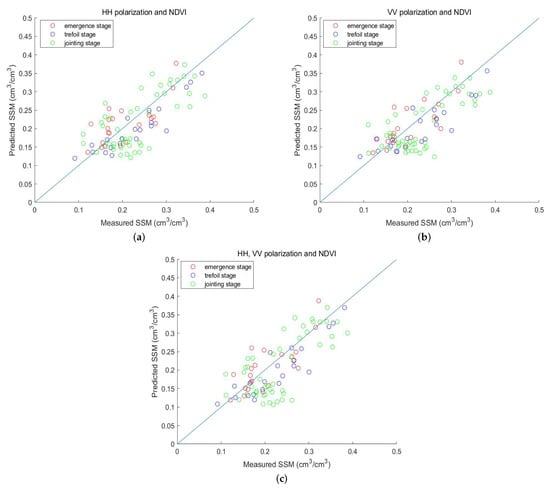
Figure 7.
Comparison of the measured SSM with retrieved SSM using three inversion configurations. (a) HH polarization and NDVI; (b) VV polarization and NDVI; (c) HH and VV polarization and NDVI.
The statistical evaluation parameters corresponding to Figure 7 are given in Table 7. Overall, the three inversion configurations have obtained good results at different vegetation growth stages, such as the maximum RMSE of 0.064 cm/cm. Besides, the MAE and R are about 0.054 cm/cm and 0.71, respectively. Among the three inversion configurations, the inversion algorithm has the highest accuracy in the trefoil stage and the lowest accuracy in the jointing stage. The values of IA and RPD indicate that the MWC-EM and ANN algorithms can accurately estimate SSM using all three inversion configurations. As observed in Table 7, the difference in accuracy is not significant under three different inversion configurations, which shows similar results using HH alone, VV alone or using VV and HH. As an example, Figure 8 gives an inversion map of the SSM when the inversion configuration is VV polarization backscattering coefficient and NDVI. Since the model in this paper is built on the corn covered area, in Figure 8, the area not covered by corn is masked. The spatiotemporal behavior of soil moisture is obvious in Figure 8. The study area is in an irrigation area, so the factors that affect the change of SSM are irrigation as well as precipitation. According to Figure 8, it can be concluded that SSM is homogeneous in the same corn field, while SSM is heterogeneous among different corn fields. This is due to the different irrigation time of different corn fields in the experimental area. When the irrigation time of a corn field is before the acquisition of Terra-SAR images and the time is similar, the SSM of this corn field in Figure 8 is high, and vice versa.
Table 7.
Statistical evaluation parameters of SSM estimates of three inversion configurations.
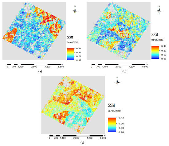
Figure 8.
SSM map with the inversion configuration of VV polarization backscattering coefficient and NDVI. (a) Emergence stage; (b) Trefoil stage; (c) Jointing stage.
5. Discussion
The validity range of different models depends on the roughness of the soil, the cultivation method and the type of vegetation [77]. According to Section 4.1, it is observed that different combined models are suitable for different stages of corn growth, while MWC-EM can effectively simulate the total backscattering coefficient in all three stages. During the emergence stage, the vegetation is in a extremely low state, at which time the effect of vegetation on the backscattering coefficient is negligible. The surface scattering of the underlying soil plays a dominant role [21]. Therefore, the empirical model combined with the two vegetation scattering models can obtain a better estimation, which indicates that the empirical model is more suitable for scattering on underlying soil than GOM. During trefoil stage, the vegetation grows to a moderate height. However, due to the large spacing of vegetation plants, they cannot cover every pixel uniformly. The WCM cannot accurately represent the influence of vegetation on the backscattering coefficient. In contrast, MWCM combined with two models of soil surface scattering can obtain higher accuracy. During the jointing stage, the vegetation coverage reached the maximum, which can be roughly regarded as covering the ground surface uniformly [21]. Therefore, the MWCM and the unmodified WCM obtained similar effects. The difference between the two models comes from interaction scattering between the underlying soil and vegetation.
The above discussion indicates that MWCM and WCM have similar potentials to describe vegetation scattering at the emergence and jointing stages. Therefore, the potential of WC-EM combined with ANN for SSM inversion is evaluated by MAE, RMSE and R. Table 8 shows the MAE, RMSE and R of SSM retrieved by WC-EM combined with ANN in each and all stages. According to Table 8, it can be concluded that the maximum RMSE is 0.071 cm/cm, which is consistent with the RMSE better than 0.08 cm/cm [23,27,44,45]. The potential of MWCM and WCM for SSM inversion can be illustrated by comparing Table 7 with Table 8. In the emergence stage, the scattering is dominated by the bare surface, so the inversion accuracy of the two models is similar. In the trefoil stage, the inversion accuracy of MWCM is better than that of WCM. At this time, due to the low vegetation coverage, MWCM can describe vegetation scattering characteristics more accurately than WCM. In the jointing period, the inversion accuracy of MWCM is slightly better than WCM, which is consistent with the results of backscattering coefficient simulation.
Table 8.
The MAE, RMSE and R of SSM retrieved by WC-EM combined with ANN in each and all stages.
According to Table 6 and Table 7, it can be concluded that both the simulation of backscattering coefficient and the inversion of SSM are more accurate in the trefoil stage than in the emergence stage. However, the lower vegetation coverage at the emergence stage than the trefoil stage suggests that the emergence stage should have a higher estimation accuracy than the trefoil stage, which is inconsistent with the experimental results. It is possibly because the temporal gap between SAR and optical data on 24 May largely affected the experimental results. Figure 2 illustrates that NDVI does not increase linearly during the three stages of corn growth. However, since it is impossible to obtain a cloud-free optical image with the same time as SAR image, only the interpolation method can be used to estimate the NDVI of SAR image acquisition date, which introduced errors in the experimental results.
Apart from soil moisture and vegetation cover, there are many factors that affect the SAR backscattering coefficient, which causes the difference between the inversion SSM and the measured SSM. Toby N. Carlson et al. [78] shows a high correlation between NDVI and vegetation cover, which weakens when vegetation cover reaches 100%. When the NDVI is greater than 0.6, the vegetation coverage has reached the maximum, while the vegetation coverage expression (Equation (11)) [52] in this paper is always less than 100%. Therefore, the inaccuracy of vegetation coverage is one of the main sources of soil moisture inversion error. Younis and Iqbal [79] point out that clay has greater water holding capacity than silt, so soil texture plays an important role in maintaining soil moisture. Simultaneously, surface temperature also affects the inversion of soil moisture [69]. However, in this experiment, the soil texture and soil temperature are only used in the Dobson model [69], which only plays a role in the interaction scattering between the underlying soil and vegetation. This is also one of the reasons for the difference between the measured value of SSM and the inversion value.
From the perspective of spatial resolution, this method can obtain soil moisture with a meter-level spatial resolution, which can be achieved in agricultural applications. The difference in SSM between different small areas can be derived from the SSM map in Figure 8, which is important for irrigated areas where complex crops are grown, compared to the kilometer-level resolution of passive microwave remote sensing [80,81]. The highest spatial resolution that can be obtained by this method is consistent with the Terra-SAR revisit cycle of 11 days, which is lower than the passive microwave remote sensing and soil moisture active passive (SMAP) [80,81]. Considering the penetration of the X-band in the vegetation layer, the effectiveness of the combined scattering model has only been verified and compared in the first three stages of corn growth. When the corn grows to the ear stage and the flowering stage, the average height of the corn is greater than 1 m, and the sensitivity between Terra-SAR backscattering coefficient and SSM is very low. Therefore, in actual agricultural applications, X-band data can only be used to estimate the SSM of the first three stages of corn growth. In order to better monitor the SSM of farmland irrigation areas, it is necessary to consider SAR satellites with longer wavelengths and shorter revisit periods in future research.
6. Conclusions
This study investigates the capability of using Terra-SAR and Landsat-7 data to retrieve SSM over agricultural soil during the three different stages of corn growth. A combined scattering model at improving the accuracy of simulation of SAR backscattering coefficient in different growth periods of corn is proposed. The proposed combined scattering model is developed based on the MWCM and an empirical model. The MWCM is used to address issues related to the the large corn plant spacing and uneven coverage during the corn growth season. The empirical model is used to solve the problem of complex expression and low precision of the bare surface scattering model. The in situ SSM measurements and remote sensing data obtained from the HiWATER are used to parameterize the combined scattering model and evaluate the potential of the model to simulate the backscattering coefficient. According to the results, it can be concluded that the combined scattering model can obtain high accuracy in the simulation of SAR backscattering coefficients at different stages of corn growth, as the maximum RMSE in the three stages is 1.0 dB, 1.0 dB and 1.3 dB respectively. Subsequently, the ANN trained by the SAR backscattering coefficient dataset synthesized by the parameterized combined scattering model is used to retrieve SSM. The comparison against ground-truth data shows that the inversion method gives acceptable results with maximum RMSE of the three corn growth stages about 0.043 cm/cm, 0.046 cm/cm, and 0.064 cm/cm respectively.
Although accurate results are obtained by using Terra-SAR and Landsat-7 data in the SSM inversion of the first three stages of corn growth in this paper, when corn is in the ear stage and after ear stage, due to the limited penetration of the X-band, there is no high sensitivity between Terra-SAR backscattering coefficient and SSM. Therefore, X-band data cannot be used for SSM inversion of dense vegetation coverage. In future studies, SSM inversion will be mainly considered for long-band (C-band and L-band) SAR data in areas with dense vegetation cover considering the entire vegetation growth period. In addition, due to the transmission of Sentinel-1 and Sentinel-2, more free data can be obtained, and the optical data and SAR data have the same spatial resolution. Therefore, in the follow-up research, we will focus on the SSM inversion of different regions and different vegetation using the Sentinel satellite.
Author Contributions
Conceptualization, X.L.; Methodology, L.Z.; Project administration, X.L.; Validation, L.Z.; Visualization, L.Z.; Writing—original draft, L.Z.; Writing—review & editing, Q.C., G.S. and J.Y. All authors have read and agreed to the published version of the manuscript.
Funding
This research was supported by the National Key R&D Program of China, grant number 2018YFC1505100, the China Academy of Railway Sciences Fund, grant number 2019YJ028, and the Key R&D Program of Shannxi, grant number 2019ZDLGY08-05.
Acknowledgments
The authors would like to acknowledge the Cold and Arid Regions Science Data Center for kindly providing the HiWATER dataset used in this work.
Conflicts of Interest
The authors declare no conflict of interest.
References
- Seneviratne, S.I.; Corti, T.; Davin, E.L.; Hirschi, M.; Jaeger, E.B.; Lehner, I.; Orlowsky, B.; Teuling, A.J. Investigating soil moisture–climate interactions in a changing climate: A review. Earth-Sci. Rev. 2010, 99, 125–161. [Google Scholar] [CrossRef]
- Moran, M.S.; Inoue, Y.; Barnes, E. Opportunities and limitations for image-based remote sensing in precision crop management. Remote Sens. Environ. 1997, 61, 319–346. [Google Scholar] [CrossRef]
- Kornelsen, K.C.; Coulibaly, P. Advances in soil moisture retrieval from synthetic aperture radar and hydrological applications. J. Hydrol. 2013, 476, 460–489. [Google Scholar] [CrossRef]
- Aubert, M.; Baghdadi, N.; Zribi, M.; Douaoui, A.; Loumagne, C.; Baup, F.; El Hajj, M.; Garrigues, S. Analysis of TerraSAR-X data sensitivity to bare soil moisture, roughness, composition and soil crust. Remote Sens. Environ. 2011, 115, 1801–1810. [Google Scholar] [CrossRef]
- Paloscia, S.; Pettinato, S.; Santi, E.; Notarnicola, C.; Pasolli, L.; Reppucci, A. Soil moisture mapping using Sentinel-1 images: Algorithm and preliminary validation. Remote Sens. Environ. 2013, 134, 234–248. [Google Scholar] [CrossRef]
- Liu, D.; Mishra, A.K.; Yu, Z. Evaluating uncertainties in multi-layer soil moisture estimation with support vector machines and ensemble Kalman filtering. J. Hydrol. 2016, 538, 243–255. [Google Scholar] [CrossRef]
- Chaparro, D.; Piles, M.; Vall-Llossera, M.; Camps, A.; Konings, A.G.; Entekhabi, D. L-band vegetation optical depth seasonal metrics for crop yield assessment. Remote Sens. Environ. 2018, 212, 249–259. [Google Scholar] [CrossRef]
- Jakobi, J.; Huisman, J.; Vereecken, H.; Diekkrüger, B.; Bogena, H. Cosmic ray neutron sensing for simultaneous soil water content and biomass quantification in drought conditions. Water Resour. Res. 2018, 54, 7383–7402. [Google Scholar] [CrossRef]
- Ghahremanloo, M.; Mobasheri, M.R.; Amani, M. Soil moisture estimation using land surface temperature and soil temperature at 5 cm depth. Int. J. Remote Sens. 2019, 40, 104–117. [Google Scholar] [CrossRef]
- Bai, X.; He, B.; Li, X.; Zeng, J.; Wang, X.; Wang, Z.; Zeng, Y.; Su, Z. First assessment of Sentinel-1A data for surface soil moisture estimations using a coupled water cloud model and advanced integral equation model over the Tibetan Plateau. Remote Sens. 2017, 9, 714. [Google Scholar] [CrossRef]
- Petropoulos, G.P.; Ireland, G.; Barrett, B. Surface soil moisture retrievals from remote sensing: Current status, products & future trends. Phys. Chem. Earth Parts A/B/C 2015, 83, 36–56. [Google Scholar]
- Pierdicca, N.; Pulvirenti, L.; Bignami, C. Soil moisture estimation over vegetated terrains using multitemporal remote sensing data. Remote Sens. Environ. 2010, 114, 440–448. [Google Scholar] [CrossRef]
- Gutman, G.; Ignatov, A. The derivation of the green vegetation fraction from NOAA/AVHRR data for use in numerical weather prediction models. Int. J. Remote Sens. 1998, 19, 1533–1543. [Google Scholar] [CrossRef]
- Yang, Y.; Guan, H.; Long, D.; Liu, B.; Qin, G.; Qin, J.; Batelaan, O. Estimation of surface soil moisture from thermal infrared remote sensing using an improved trapezoid method. Remote Sens. 2015, 7, 8250–8270. [Google Scholar] [CrossRef]
- Sadeghi, M.; Babaeian, E.; Tuller, M.; Jones, S.B. The optical trapezoid model: A novel approach to remote sensing of soil moisture applied to Sentinel-2 and Landsat-8 observations. Remote Sens. Environ. 2017, 198, 52–68. [Google Scholar] [CrossRef]
- Zhao, W.; Sánchez, N.; Li, A. Triangle Space-Based Surface Soil Moisture Estimation by the Synergistic Use of In Situ Measurements and Optical/Thermal Infrared Remote Sensing: An Alternative to Conventional Validations. IEEE Trans. Geosci. Remote Sens. 2018, 56, 4546–4558. [Google Scholar] [CrossRef]
- Baghdadi, N.; Zribi, M.; Loumagne, C.; Ansart, P.; Anguela, T.P. Analysis of TerraSAR-X data and their sensitivity to soil surface parameters over bare agricultural fields. Remote Sens. Environ. 2008, 112, 4370–4379. [Google Scholar] [CrossRef]
- Barrett, B.W.; Dwyer, E.; Whelan, P. Soil moisture retrieval from active spaceborne microwave observations: An evaluation of current techniques. Remote Sens. 2009, 1, 210–242. [Google Scholar] [CrossRef]
- Narvekar, P.S.; Entekhabi, D.; Kim, S.B.; Njoku, E.G. Soil moisture retrieval using L-band radar observations. IEEE Trans. Geosci. Remote Sens. 2015, 53, 3492–3506. [Google Scholar] [CrossRef]
- Zheng, D.; van der Velde, R.; Wen, J.; Wang, X.; Ferrazzoli, P.; Schwank, M.; Colliander, A.; Bindlish, R.; Su, Z. Assessment of the SMAP soil emission model and soil moisture retrieval algorithms for a Tibetan Desert ecosystem. IEEE Trans. Geosci. Remote Sens. 2018, 56, 3786–3799. [Google Scholar] [CrossRef]
- Xing, M.; He, B.; Ni, X.; Wang, J.; An, G.; Shang, J.; Huang, X. Retrieving Surface Soil Moisture over Wheat and Soybean Fields during Growing Season Using Modified Water Cloud Model from Radarsat-2 SAR Data. Remote Sens. 2019, 11, 1956. [Google Scholar] [CrossRef]
- Bazzi, H.; Baghdadi, N.; El Hajj, M.; Zribi, M.; Belhouchette, H. A Comparison of Two Soil Moisture Products S 2 MP and Copernicus-SSM Over Southern France. IEEE J. Sel. Top. Appl. Earth Obs. Remote Sens. 2019, 12, 3366–3375. [Google Scholar] [CrossRef]
- El Hajj, M.; Baghdadi, N.; Zribi, M. Comparative analysis of the accuracy of surface soil moisture estimation from the C-and L-bands. Int. J. Appl. Earth Obs. Geoinf. 2019, 82, 101888. [Google Scholar] [CrossRef]
- Bousbih, S.; Zribi, M.; El Hajj, M.; Baghdadi, N.; Lili-Chabaane, Z.; Gao, Q.; Fanise, P. Soil moisture and irrigation mapping in A semi-arid region, based on the synergetic use of Sentinel-1 and Sentinel-2 data. Remote Sens. 2018, 10, 1953. [Google Scholar] [CrossRef]
- El Hajj, M.; Baghdadi, N.; Zribi, M.; Bazzi, H. Synergic use of Sentinel-1 and Sentinel-2 images for operational soil moisture mapping at high spatial resolution over agricultural areas. Remote Sens. 2017, 9, 1292. [Google Scholar] [CrossRef]
- Gao, Q.; Zribi, M.; Escorihuela, M.J.; Baghdadi, N. Synergetic use of Sentinel-1 and Sentinel-2 data for soil moisture mapping at 100 m resolution. Sensors 2017, 17, 1966. [Google Scholar] [CrossRef]
- El Hajj, M.; Baghdadi, N.; Zribi, M.; Belaud, G.; Cheviron, B.; Courault, D.; Charron, F. Soil moisture retrieval over irrigated grassland using X-band SAR data. Remote Sens. Environ. 2016, 176, 202–218. [Google Scholar] [CrossRef]
- Baghdadi, N.; Camus, P.; Beaugendre, N.; Issa, O.M.; Zribi, M.; Desprats, J.F.; Rajot, J.L.; Abdallah, C.; Sannier, C. Estimating surface soil moisture from TerraSAR-X data over two small catchments in the Sahelian Part of Western Niger. Remote Sens. 2011, 3, 1266–1283. [Google Scholar] [CrossRef]
- Baghdadi, N.; Cresson, R.; El Hajj, M.; Ludwig, R.; La Jeunesse, I. Estimation of soil parameters over bare agriculture areas from C-band polarimetric SAR data using neural networks. Hydrol. Earth Syst. Sci. 2012, 16, 1607–1621. [Google Scholar] [CrossRef]
- Srivastava, H.S.; Patel, P.; Sharma, Y.; Navalgund, R.R. Large-area soil moisture estimation using multi-incidence-angle RADARSAT-1 SAR data. IEEE Trans. Geosci. Remote Sens. 2009, 47, 2528–2535. [Google Scholar] [CrossRef]
- Fung, A.K.; Li, Z.; Chen, K.S. Backscattering from a randomly rough dielectric surface. IEEE Trans. Geosci. Remote Sens. 1992, 30, 356–369. [Google Scholar] [CrossRef]
- Ulaby, F.T.; Moore, R.K.; Fung, A.K. Microwave Remote Sensing: Active and Passive. Volume 3—From Theory to Applications; Artech House, Inc.: Norwood, MA, USA, 1986. [Google Scholar]
- Sancer, M. Shadow-corrected electromagnetic scattering from a randomly rough surface. IEEE Trans. Antennas Propag. 1969, 17, 577–585. [Google Scholar] [CrossRef]
- Oh, Y.; Sarabandi, K.; Ulaby, F.T. Semi-empirical model of the ensemble-averaged differential Mueller matrix for microwave backscattering from bare soil surfaces. IEEE Trans. Geosci. Remote Sens. 2002, 40, 1348–1355. [Google Scholar] [CrossRef]
- Shi, J.; Wang, J.; Hsu, A.Y.; O’Neill, P.E.; Engman, E.T. Estimation of bare surface soil moisture and surface roughness parameter using L-band SAR image data. IEEE Trans. Geosci. Remote Sens. 1997, 35, 1254–1266. [Google Scholar]
- Rao, K.; Raju, S.; Wang, J.R. Estimation of soil moisture and surface roughness parameters from backscattering coefficient. IEEE Trans. Geosci. Remote Sens. 1993, 31, 1094–1099. [Google Scholar] [CrossRef]
- Oh, Y.; Sarabandi, K.; Ulaby, F.T. An empirical model and an inversion technique for radar scattering from bare soil surfaces. IEEE Trans. Geosci. Remote Sens. 1992, 30, 370–381. [Google Scholar] [CrossRef]
- Dubois, P.C.; Van Zyl, J.; Engman, T. Measuring soil moisture with imaging radars. IEEE Trans. Geosci. Remote Sens. 1995, 33, 915–926. [Google Scholar] [CrossRef]
- Baghdadi, N.; Choker, M.; Zribi, M.; Hajj, M.E.; Paloscia, S.; Verhoest, N.E.; Lievens, H.; Baup, F.; Mattia, F. A new empirical model for radar scattering from bare soil surfaces. Remote Sens. 2016, 8, 920. [Google Scholar] [CrossRef]
- Shi, J.; Du, Y.; Du, J.; Jiang, L.; Chai, L.; Mao, K.; Xu, P.; Ni, W.; Xiong, C.; Liu, Q.; et al. Progresses on microwave remote sensing of land surface parameters. Sci. China Earth Sci. 2012, 55, 1052–1078. [Google Scholar] [CrossRef]
- Ulaby, F.T.; Sarabandi, K.; Mcdonald, K.; Whitt, M.; Dobson, M.C. Michigan microwave canopy scattering model. Int. J. Remote Sens. 1990, 11, 1223–1253. [Google Scholar] [CrossRef]
- Attema, E.; Ulaby, F.T. Vegetation modeled as a water cloud. Radio Sci. 1978, 13, 357–364. [Google Scholar] [CrossRef]
- McDonald, K.C.; Dobson, M.C.; Ulaby, F.T. Using MIMICS to model L-band multiangle and multitemporal backscatter from a walnut orchard. IEEE Trans. Geosci. Remote Sens. 1990, 28, 477–491. [Google Scholar] [CrossRef]
- De Roo, R.D.; Du, Y.; Ulaby, F.T.; Dobson, M.C. A semi-empirical backscattering model at L-band and C-band for a soybean canopy with soil moisture inversion. IEEE Trans. Geosci. Remote Sens. 2001, 39, 864–872. [Google Scholar] [CrossRef]
- Baghdadi, N.; El Hajj, M.; Zribi, M.; Bousbih, S. Calibration of the water cloud model at C-band for winter crop fields and grasslands. Remote Sens. 2017, 9, 969. [Google Scholar] [CrossRef]
- Tomer, S.K.; Al Bitar, A.; Sekhar, M.; Zribi, M.; Bandyopadhyay, S.; Sreelash, K.; Sharma, A.K.; Corgne, S.; Kerr, Y. Retrieval and multi-scale validation of soil moisture from multi-temporal SAR data in a semi-arid tropical region. Remote Sens. 2015, 7, 8128–8153. [Google Scholar] [CrossRef]
- Pathe, C.; Wagner, W.; Sabel, D.; Doubkova, M.; Basara, J. Using Envisat ASAR Global Mode data for Surface Soil Moisture Retrieval over Oklahoma (USA) using a change detection approach. In Proceedings of the EGU General Assembly Conference Abstracts, Vienna, Austria, 19–24 April 2009; Volume 11, p. 4921. [Google Scholar]
- Mirsoleimani, H.R.; Sahebi, M.R.; Baghdadi, N.; El Hajj, M. Bare soil surface moisture retrieval from sentinel-1 SAR data based on the calibrated IEM and dubois models using neural networks. Sensors 2019, 19, 3209. [Google Scholar] [CrossRef]
- Baghdadi, N.; Gaultier, S.; King, C. Retrieving surface roughness and soil moisture from SAR data using neural networks. In Proceedings of the Retrieval of Bio-and Geo-Physical Parameters from SAR Data for Land Applications, Sheffield, UK, 11–14 September 2001; Volume 475, pp. 315–319. [Google Scholar]
- Zribi, M.; Kotti, F.; Amri, R.; Wagner, W.; Shabou, M.; Lili-Chabaane, Z.; Baghdadi, N. Soil moisture mapping in a semiarid region, based on ASAR/Wide Swath satellite data. Water Resour. Res. 2014, 50, 823–835. [Google Scholar] [CrossRef]
- Chai, S.S.; Walker, J.P.; Makarynskyy, O.; Kuhn, M.; Veenendaal, B.; West, G. Use of soil moisture variability in artificial neural network retrieval of soil moisture. Remote Sens. 2010, 2, 166–190. [Google Scholar] [CrossRef]
- Tao, L.; Wang, G.; Chen, W.; Chen, X.; Li, J.; Cai, Q. Soil moisture retrieval from SAR and optical data using a combined model. IEEE J. Sel. Top. Appl. Earth Obs. Remote Sens. 2019, 12, 637–647. [Google Scholar] [CrossRef]
- Li, X.; Cheng, G.; Liu, S.; Xiao, Q.; Ma, M.; Jin, R.; Che, T.; Liu, Q.; Wang, W.; Qi, Y.; et al. Heihe watershed allied telemetry experimental research (HiWATER): Scientific objectives and experimental design. Bull. Am. Meteorol. Soc. 2013, 94, 1145–1160. [Google Scholar] [CrossRef]
- Li, X.; Liu, S.; Xiao, Q.; Ma, M.; Jin, R.; Che, T.; Wang, W.; Hu, X.; Xu, Z.; Wen, J.; et al. A multiscale dataset for understanding complex eco-hydrological processes in a heterogeneous oasis system. Sci. Data 2017, 4, 170083. [Google Scholar] [CrossRef] [PubMed]
- Jin, R.; Li, X.; Yan, B.; Li, X.; Luo, W.; Ma, M.; Guo, J.; Kang, J.; Zhu, Z.; Zhao, S. A nested ecohydrological wireless sensor network for capturing the surface heterogeneity in the midstream areas of the Heihe River Basin, China. IEEE Geosci. Remote Sens. Lett. 2014, 11, 2015–2019. [Google Scholar] [CrossRef]
- Xufeng, W.; Mingguo, M. HiWATER: Dataset of soil parameters in the midstream of the Heihe River Basin (2012). Digital Heihe 2017. [Google Scholar] [CrossRef]
- Qiu, J.; Crow, W.T.; Wagner, W.; Zhao, T. Effect of vegetation index choice on soil moisture retrievals via the synergistic use of synthetic aperture radar and optical remote sensing. Int. J. Appl. Earth Obs. Geoinf. 2019, 80, 47–57. [Google Scholar] [CrossRef]
- Mingguo, M.; Jun, L. HiWATER: BNUNET soil moisture and LST observation dataset in the midstream of the Heihe River Basin (2012). Digital Heihe 2016. [Google Scholar] [CrossRef]
- Kang, J.; Li, X.; Jin, R.; Ge, Y.; Wang, J.; Wang, J. Hybrid optimal design of the eco-hydrological wireless sensor network in the middle reach of the Heihe River Basin, China. Sensors 2014, 14, 19095–19114. [Google Scholar] [CrossRef]
- Mingguo, M.; Cunhui, D.; Xin, L. HiWATER: WATERNET observation dataset in the middle of Heihe River Basin (2012). Digital Heihe 2015. [Google Scholar] [CrossRef]
- Mingguo, M.; Cunhui, D.; Xin, L.; Dazhi, L. HiWATER: SoilNET observation dataset in the midstream of the Heihe River Basin. Digital Heihe 2014. [Google Scholar] [CrossRef]
- Jing, W.; Mingguo, M.; Jinxin, Z.; Xin, L. HiWATER: Dataset of plant height observed in the midstream of the Heihe River Basin. Digital Heihe 2017. [Google Scholar] [CrossRef]
- Baghdadi, N.N.; El Hajj, M.; Zribi, M.; Fayad, I. Coupling SAR C-band and optical data for soil moisture and leaf area index retrieval over irrigated grasslands. IEEE J. Sel. Top. Appl. Earth Obs. Remote Sens. 2015, 9, 1229–1243. [Google Scholar] [CrossRef]
- Eineder, M.; Fritz, T.; Mittermayer, J.; Roth, A.; Boerner, E.; Breit, H. Terrasar-X Ground Segment, Basic Product Specification Document; Technical Report; Cluster Applied Remote Sensing (Caf) Oberpfaffenhofen: Munich, Germany, 2008. [Google Scholar]
- Wang, S.; Li, X.; Han, X.; Jin, R. Estimation of surface soil moisture and roughness from multi-angular ASAR imagery in the Watershed Allied Telemetry Experimental Research (WATER). Hydrol. Earth Syst. Sci. 2011, 15, 1415–1426. [Google Scholar] [CrossRef]
- Anguela, T.P.; Zribi, M.; Baghdadi, N.; Loumagne, C. Analysis of local variation of soil surface parameters with TerraSAR-X radar data over bare agricultural fields. IEEE Trans. Geosci. Remote Sens. 2009, 48, 874–881. [Google Scholar] [CrossRef]
- Shi, J.; Lee, J.S.; Chen, K.; Sun, Q. Evaluate usage of decomposition technique in estimation of soil moisture with vegetated surface by multi-temporal measurements. In Proceedings of the IEEE 2000 International Geoscience and Remote Sensing Symposium, Honolulu, HI, USA, 24–28 July 2000; Volume 3, pp. 1098–1100. [Google Scholar]
- Du, J.; Shi, J.; Sun, R. The development of HJ SAR soil moisture retrieval algorithm. Int. J. Remote Sens. 2010, 31, 3691–3705. [Google Scholar] [CrossRef]
- El-Hajj, M.; Baghdadi, N.; Belaud, G.; Zribi, M.; Cheviron, B.; Courault, D.; Charron, F. Soil moisture retrieval over grassland using X-band SAR data. In Proceedings of the 2014 IEEE Geoscience and Remote Sensing Symposium, Quebec City, QC, Canada, 13–18 July 2014; pp. 3638–3641. [Google Scholar]
- Woodhouse, I.H.; Hoekman, D.H. Determining land-surface parameters from the ERS wind scatterometer. IEEE Trans. Geosci. Remote Sens. 2000, 38, 126–140. [Google Scholar] [CrossRef]
- Wen, J.; Su, Z. The estimation of soil moisture from ERS wind scatterometer data over the Tibetan plateau. Phys. Chem. Earth Parts A/B/C 2003, 28, 53–61. [Google Scholar] [CrossRef]
- Frison, P.L.; Mougin, E.; Hiernaux, P. Observations and simulations of the ERS wind scatterometer response over a Sahelian region. In Proceedings of the 1997 IEEE International Geoscience and Remote Sensing Symposium, Singapore, 3–8 August 1997; Volume 4, pp. 1832–1834. [Google Scholar]
- Kseneman, M.; Gleich, D.; Cucej, Ž. Soil moisture estimation using high-resolution spotlight TerraSAR-X data. IEEE Geosci. Remote Sens. Lett. 2011, 8, 686–690. [Google Scholar] [CrossRef]
- Dobson, M.C.; Ulaby, F.T. Active microwave soil moisture research. IEEE Trans. Geosci. Remote Sens. 1986, GE-24, 23–36. [Google Scholar] [CrossRef]
- Kseneman, M.; Gleich, D. Soil-moisture estimation from X-band data using Tikhonov regularization and neural net. IEEE Trans. Geosci. Remote Sens. 2013, 51, 3885–3898. [Google Scholar] [CrossRef]
- Farifteh, J.; Van der Meer, F.; Atzberger, C.; Carranza, E. Quantitative analysis of salt-affected soil reflectance spectra: A comparison of two adaptive methods (PLSR and ANN). Remote Sens. Environ. 2007, 110, 59–78. [Google Scholar] [CrossRef]
- Zribi, M.; Muddu, S.; Bousbih, S.; Al Bitar, A.; Tomer, S.K.; Baghdadi, N.; Bandyopadhyay, S. Analysis of L-band SAR data for soil moisture estimations over agricultural areas in the tropics. Remote Sens. 2019, 11, 1122. [Google Scholar] [CrossRef]
- Carlson, T.N.; Gillies, R.R.; Perry, E.M. A method to make use of thermal infrared temperature and NDVI measurements to infer surface soil water content and fractional vegetation cover. Remote Sens. Rev. 1994, 9, 161–173. [Google Scholar] [CrossRef]
- Younis, S.M.Z.; Iqbal, J. Estimation of soil moisture using multispectral and FTIR techniques. Egypt. J. Remote Sens. Space Sci. 2015, 18, 151–161. [Google Scholar] [CrossRef]
- Zhu, Q.; Luo, Y.; Xu, Y.P.; Tian, Y.; Yang, T. Satellite soil moisture for agricultural drought monitoring: Assessment of SMAP-derived soil water deficit index in Xiang River Basin, China. Remote Sens. 2019, 11, 362. [Google Scholar] [CrossRef]
- Bai, L.; Lv, X.; Li, X. Evaluation of Two SMAP Soil Moisture Retrievals Using Modeled-and Ground-Based Measurements. Remote Sens. 2019, 11, 2891. [Google Scholar] [CrossRef]


© 2020 by the authors. Licensee MDPI, Basel, Switzerland. This article is an open access article distributed under the terms and conditions of the Creative Commons Attribution (CC BY) license (http://creativecommons.org/licenses/by/4.0/).