Article

Using UAV-Based SOPC Derived LAI and SAFY Model for Biomass and Yield Estimation of Winter Wheat

1
Department of Geography, The University of Western Ontario, London, ON N6A 5C2, Canada
2
Ottawa Research and Development Centre, Agriculture and Agri-Food Canada, Ottawa, ON K1A 0C6, Canada
*
Author to whom correspondence should be addressed.
Remote Sens. 2020, 12(15), 2378; https://doi.org/10.3390/rs12152378
Submission received: 18 June 2020 / Revised: 16 July 2020 / Accepted: 21 July 2020 / Published: 24 July 2020
(This article belongs to the Special Issue Environmental Mapping Using Remote Sensing)

Abstract

:
Knowledge of sub-field yield potential is critical for guiding precision farming. The recently developed simulated observation of point cloud (SOPC) method can generate high spatial resolution winter wheat effective leaf area index (SOPC-LAIe) maps from the unmanned aerial vehicle (UAV)-based point cloud data without ground-based measurements. In this study, the SOPC-LAIe maps, for the first time, were applied to the simple algorithm for yield estimation (SAFY) to generate the sub-field biomass and yield maps. First, the dry aboveground biomass (DAM) measurements were used to determine the crop cultivar-specific parameters and simulated green leaf area index (LAI) in the SAFY model. Then, the SOPC-LAIe maps were converted to green LAI using a normalization approach. Finally, the multiple SOPC-LAIe maps were applied to the SAFY model to generate the final DAM and yield maps. The root mean square error (RMSE) between the estimated and measured yield is 88 g/m2, and the relative root mean squire error (RRMSE) is 15.2%. The pixel-based DAM and yield map generated in this study revealed clearly the within-field yield variation. This framework using the UAV-based SOPC-LAIe maps and SAFY model could be a simple and low-cost alternative for final yield estimation at the sub-field scale.

1. Introduction

Precision agriculture aims at optimizing input and output in field operations in order to achieve maximum economic profit while maintain environmental sustainability [1]. The sub-field level crop monitoring can provide finer spatial resolution (meter level) information and reveal the within-field crop variability. Information on the spatial variation of crop biomass and yield at the sub-field level is directly relevant to increasing farm profit by addressing the low-productivity areas within a field. Remote sensing has long been recognized as an effective means to provide multi-temporal information on crop growth over large areas in support of precision agriculture [2,3,4]. For example, moderate resolution imaging spectroradiometer (MODIS), Landsat, and RapidEye optical satellite data have been used to monitor crop growth status throughout the growing season using vegetation spectral indices and crop models [5,6,7,8]. Although the spatial and temporal resolution of satellite imagery has been improved over the years, it is still incapable of providing timely and detailed information of within-field variations for operational applications [9]. The recent advancement of the unmanned aerial vehicle (UAV) system has overcome the spatial and temporal limitation of satellite data for precision agriculture [10,11,12]. The high spatial and temporal UAV-based imagery can provide important information for monitoring the within-field variabilities of crop status during the growing season [13,14]. The high quality and real-time UAV data gives a better solution in precision farming management, such as the monitoring of crop canopy leaf area index (LAI), nitrogen status, water stress, weed stress, and dry aboveground biomass [15,16,17,18].
Commonly, two categories of approaches have been adopted in using remote sensing data for crop biomass and yield estimation. Empirical models are the earliest and simplest approaches to estimate crop yield from remotely sensed imagery and have still been used in many recent applications [5,19,20,21,22,23,24,25]. The basic idea of the empirical models in crop yield estimation relies on the regression between in-situ measurements and remote sensing observations [26,27]. In recent years, many studies have attempted to obtain crop yield estimation using machine learning algorithms [28,29]. However, these empirical relationships are location, time, and crop type dependent and hence limit their operational applications to different crop types and over dynamic geographical regions [30,31]. For example, Yue et al. (2019) [32] estimated the winter wheat dry aboveground biomass (DAM) from the ground based hyperspectral vegetation index with a root mean square error (RMSE) of 1.22 t/ha (122 g/m2). The ground measurements and spectral calibration were required to establish the specific relationship at this location between vegetation index and DAM. On the contrary, crop growth models have been developed by combining crop and environmental parameters to simulate crop growth and estimate crop biomass [33,34]. For modeling approach, remote sensing data have been used for model calibration and initialization. The main challenge of the modeling approach is that many model parameters are difficult to obtain, especially for process-based models [35,36,37]. Currently, crop growth models such as AquaCrop [38], Simulateur mulTIdisciplinaire pour les Cultures Standard (STICS) [33], and World Food Studies (WOFOST) [39] have been well developed in crop production estimation. However, these models require a comprehensive set of parameters to simulate crop growth status. For example, WOFOST requires about 40 parameters and the data acquisition is labor and time intensive, which is challenging to apply in practice. Furthermore, model calibration can introduce uncertainties due to errors contained in remote sensing data products and in-situ measurements.
In general, process-based models that can accurately describe crop growth processes have better model performances. However, they require more complex calculations compared to the empirical methods [40]. The simple algorithm for yield (SAFY) model is a semi-empirical crop model, which combines the crop light use efficiency (LUE) theory [41] and leaf partitioning function [42] to estimate the daily increase in green leaf area index (GLAI) and DAM. SAFY has the benefit of model simplicity yet maintaining the required biophysical processes of leaf growth and senescence [43]. It has been widely adopted in estimating crop biomass and yield using satellite imagery derived LAI for model calibration [5,34,36,40]. The input parameters of the SAFY model include crop phenology, cultivar-specific parameters (CSPs) such as effective light-use efficiency (ELUE), fraction of green leaves, total DAM, and weather data. Usually, LAI derived from remote sensing is used for model calibration. Different estimation approaches can produce different terms of LAI, such as GLAI, effective LAI (LAIe), actual LAI, and plant area index [44], which will lead to a different CSPs for the SAFY model. Therefore, LAI normalization is a necessary procedure for SAFY model calibration in order to achieve accurate crop biomass and yield estimation.
The light-weight UAV system combined with the light-weight multispectral camera has been used to provide the spectral information for crop field during the growing season in LAI and DAM monitoring [15,27,45,46]. Zhou et al. (2017) [27] addressed the fact that the uav-based normalized difference vegetation index (NDVI) has a linear relationship with LAI in rice, with an R2 of 0.71. Although the principle of the vegetation indices is simple, it requires accurate radiometric correction. The accuracy of the vegetation index will be influenced by some other factors, such as shadow and illumination. In addition, the multispectral or hyperspectral camera is more expensive than the regular RGB camera and it also requires a larger UAV system, which will be difficult in practice for farmers. In contrast, the recently developed simulated observation of point cloud (SOPC) method uses the UAV-based point cloud data derived from low-cost RGB imagery to calculated gap fraction of crop canopy from the ratio of bare ground points and the total number of the points in simulated observation area, and can automatically generate LAIe maps showing within field variation [47]. The LAIe is the result of the indirect approach retrieved LAI value using a non-destructive method. If the canopy satisfies the assumption of a random spatial distribution, the LAIe could be calculated from the gap fraction of the canopy [48]. The UAV-based photogrammetry point cloud data contains crop structural information. The SOPC derived LAIe maps from the UAV-based point cloud data can clearly indicate the winter wheat LAIe spatial variability without using ground based LAIe measurements. In addition, the SOPC method is not affected by shadow and illumination, which does not require a radiometric calibration for UAV-based imagery. Currently, Canada has no restriction on UAV system less than 25 kg in agricultural operating. This may encourage the end users to adopt the innovative technology in crop monitoring. The demand for crop monitoring will require a low-cost and accessible approach to achieve the estimation of crop DAM and yield for farmers. Due to the low-cost and easy operation of SOPC method, the SOPC derived LAIe has a great potential for final DAM and yield estimation.
The overall objective of this study aims at developing a simple and low-cost UAV-based approach for generating a high-resolution final DAM and yield maps without ground-based measurements. The SOPC derived UAV-based point cloud LAIe (SOPC-LAIe) were applied to the SAFY model, using winter wheat as an example, to generate the final DAM and yield map to represent the DAM and yield spatial variabilities. The study is designed: (1) to determine winter wheat CSPs from DAM in the SAFY calibration instead of LAI measurements, (2) to generate high spatial resolution multi-temporal LAI maps using the newly developed SOPC method on UAV-based point cloud data, and (3) to generate winter wheat final DAM and yield map using SAFY model calibrated with the UAV-based LAIe maps.

2. Materials and Methods

2.1. Study Area

The study site locates in the west of Melbourne, southwestern Ontario, Canada (42.787707° N, 81.594801° W) (Figure 1a). This region has productive soil and abundant water supply. Due to its long cold winter and shorter growing season (April to September), there is only one harvest per year for field crops. Winter wheat is one of the major crops grown in this region, which is typically sown in the previous fall and regrow in the following spring after snowmelt. The selected winter wheat field is 41 acres in size. The soft red winter wheat cultivar (Brevant Branson, Corteva Agriscience, Wilmington, DE, USA) was planted on 12 October 2018, and harvested on 26 July 2019. The plant emergence date was observed in the field on 19 December 2018(64 days after planting).

2.2. Field Sampling Design and Field Data Collection

Since the UAV imagery was to be collected at very high spatial resolution, the corresponding destructive biomass collection will affect the subsequent crop parameter measurements. To circumvent this situation, two sub-fields, S1 and S2, were selected within this winter wheat field (Figure 1b). S1 was used to collect LAI and DAM, and S2 was used to collect other crop parameters, including LAI, crop height, phenology, and final DAM. The size of each subfield is 100 m by 200 m. The blue points were the sampling locations in S1, and the red points were the sampling locations in S2.
Fieldwork was conducted multiple times from 11 May to 22 July in 2019. In S1, destructive aboveground biomass samples were collected at each of the 12 sampling locations on 8 May, 17 May, 21 May, 27 May, 3 June, 11 June, and 20 July. Winter wheat plant samples were collected from two 0.5 m by 0.5 sections within a 4 × 4 m area at each sampling location. The fresh plant samples were placed in plastic bags and transferred back to the lab directly. All samples were oven dried at 80 °C for at least 24 h to obtain the DAM. In S2, 32 sampling points were used to collect other data, including LAI, soil moisture, crop height and phenology on 11 May, 21 May, 27 May, 3 June, and 11 June. At each sampling location, LAI was obtained using a Nikon D300s camera and a 10.5mm fisheye lens following the procedures described in Shang et al. (2014). Crop phenology was identified in the field using the Biologische Bundesanstalt, Bundessortenamt und CHemische Industrie (BBCH) scale. Details on data collection are listed in Table 1.

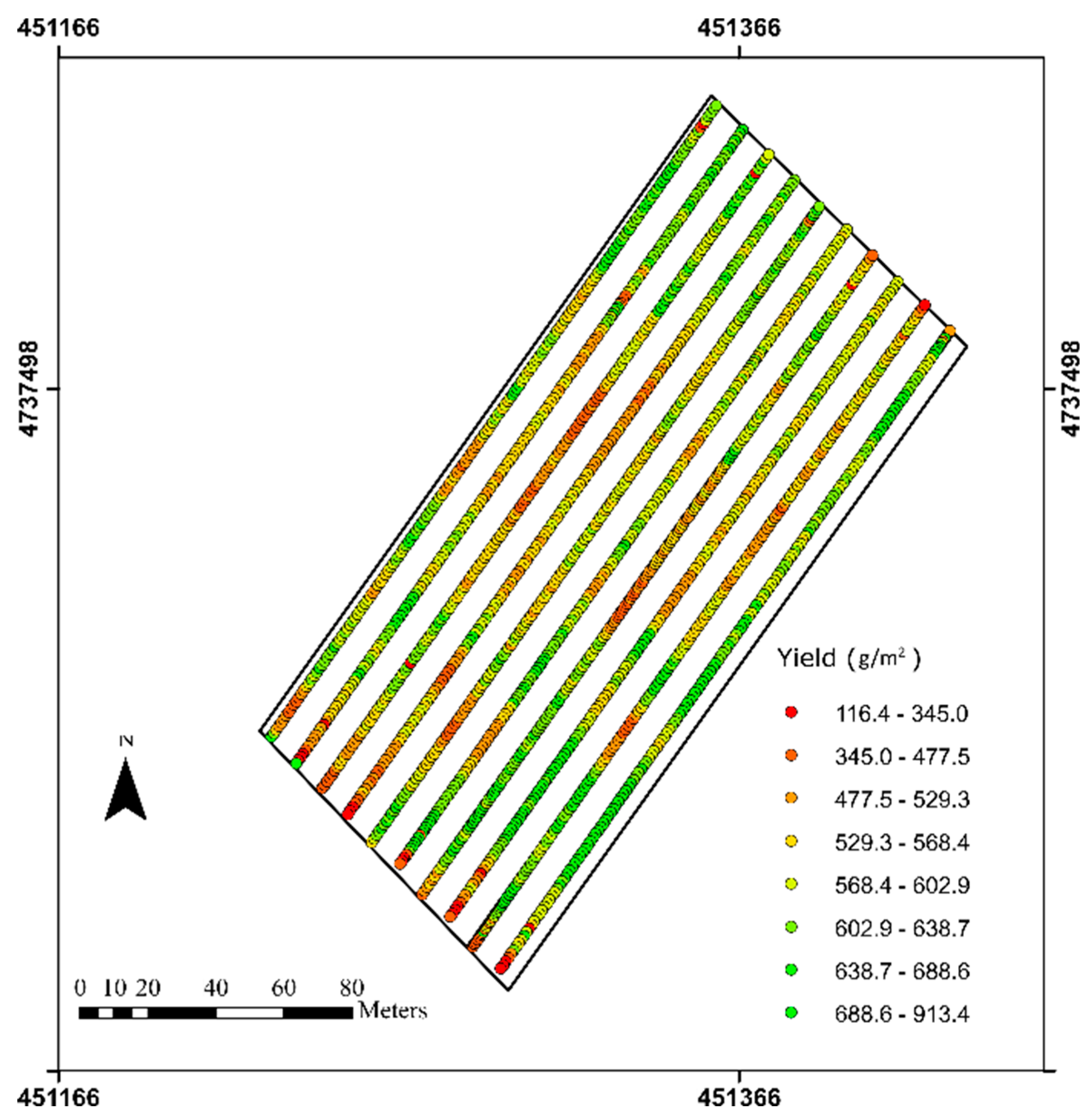
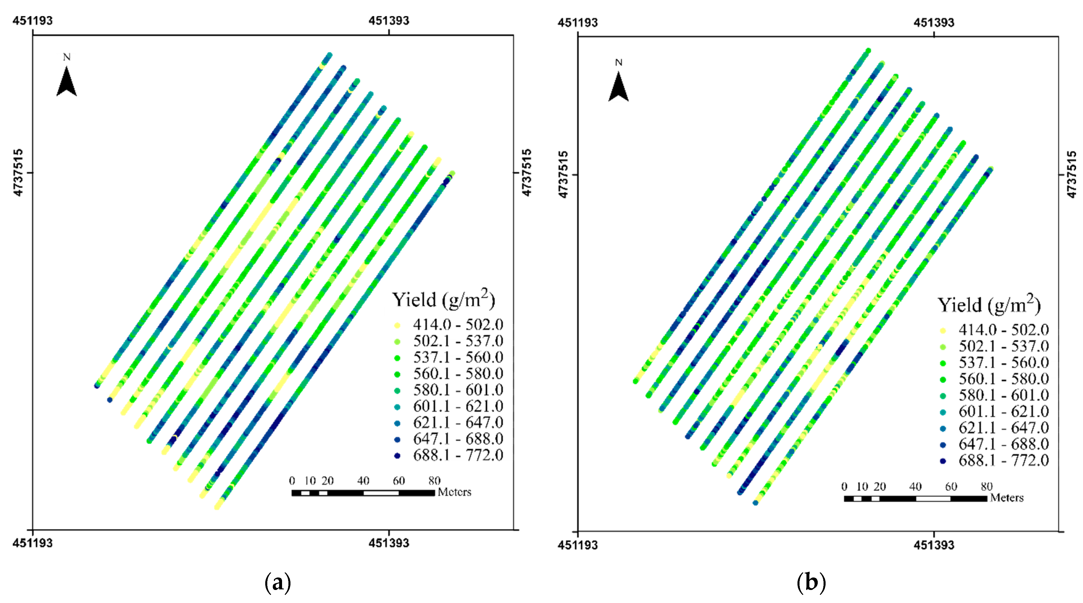
2.3. Combine Harvester Yield Data Collection

The true spatially variable winter wheat yield data was collected by the producer using a 10-m swath John Deere Combine Harvester (John Deere, USA). This harvester equipped with a grain yield monitor and real-time kinematic (RTK)-global navigation satellite systems (GNSS) to record the dry grain weight every second and measured the harvested mass flow, moisture content, and geographic position, in addition to generating high spatial resolution yield map. The moving area of the combine harvester will be calculated by multiplying the harvester moving speed and time interval during crop weight recording. The yield map for S2 was composed of many points containing the yield values (Figure 2). The yield data were then processed in ArcMap 10.7 (ESRI, USA) for duplicate-point removal, spatial resampling, and data extraction.

2.4. UAV-Based Image Collection

Multi-temporal UAV-based RGB imagery was collected using a DJI phantom 4 RTK UAV system on 11 May, 21 May, and 27 May when crop phenology was at BBCH scale were 21, 31, and 39 of early leaf development stage to the end of the stem extension stage for S2. A 5K high-resolution digital camera was mounted on this system to collect information on red, green, and blue bands. An RTK base station was placed on the ground and combined with the RTK system on the UAV to achieve high precision location estimation for all imagery. The UAV flights were performed between 10 am and 2 pm and flown at the altitude of 30 m with the front and side overlapping of 90%. The total time of the operation is 55 min to acquire all images for S2. The Pix4Dmapper Pro v2.4 (Pix4D, Lausanne, Switzerland) software was used to process the UAV-based imagery to generate 3D point cloud data (PCD). The time of point cloud generation and LAIe calculation depends on the hardware of computer. It took about 30 h with a 12 core XEON processor and Quadro M4000 video card for this field in this study. The output of the 3D PCD has a similar format to LiDAR data, which contained the crop structure and optical RGB information. This type of PCD has a low cost on both sensor and UAV system.

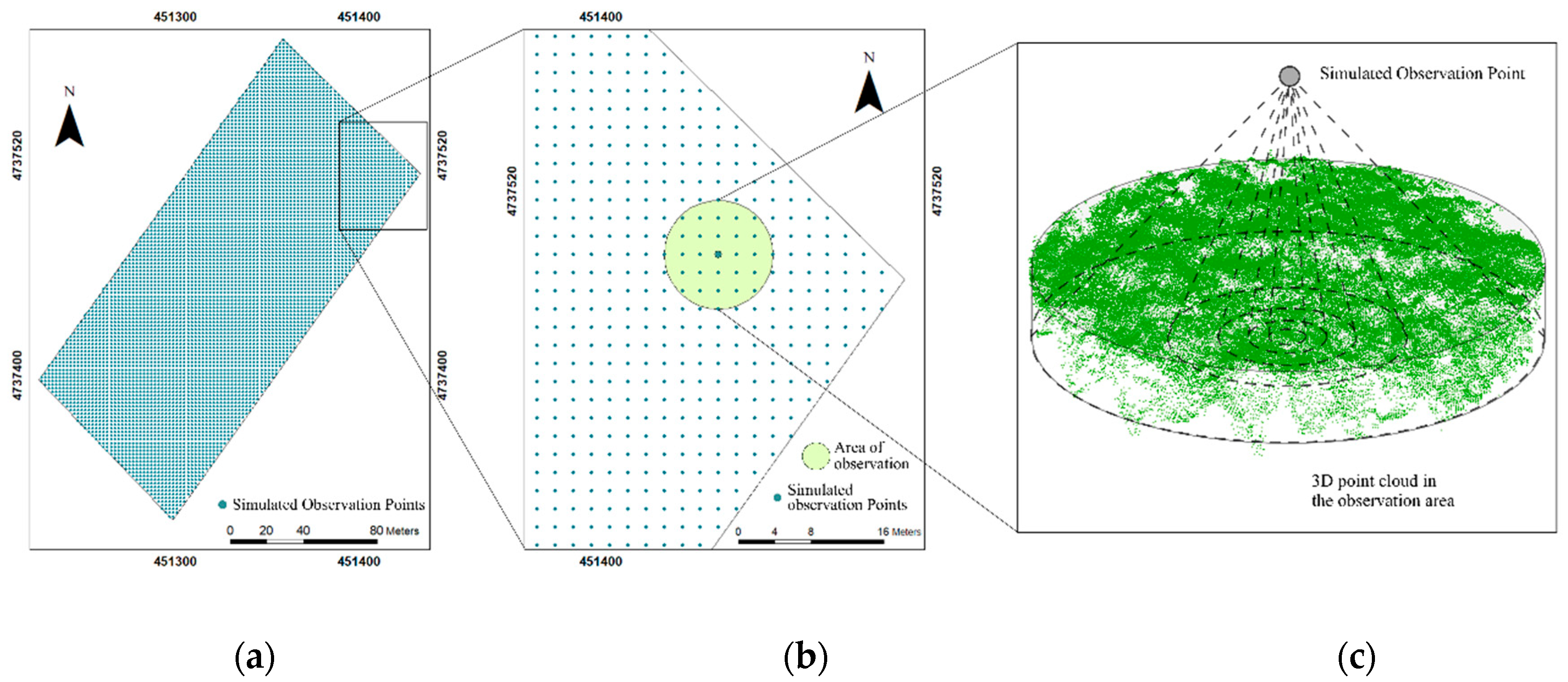
2.5. Simulated Observation of Point Cloud Method
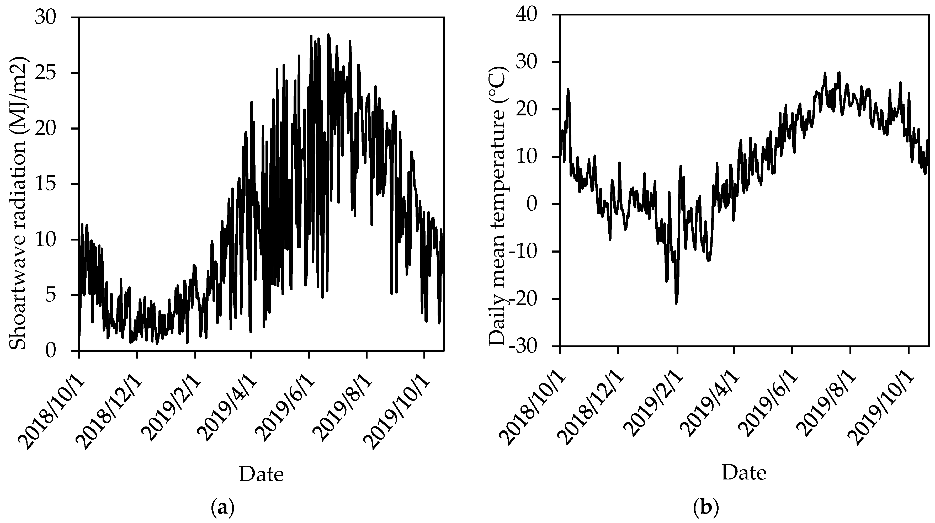
The SOPC method was designed to retrieve the spatial distribution of crop canopy and bare ground points in a simulated observation area from the UAV-based PCD and generate high spatial resolution crop LAIe map [47]. First, the SOPC method divided the study area into many observation areas based on the final resolution of LAI map. In each simulate area, the crop vegetation and bare ground points in the UAV-based PCD will be classified into two groups. The gap fraction will be calculated from the ratio of crop canopy and bare ground points at multi-view angles. Finally, the LAIe will be calculated from the gap fraction in the simulate area. The general principle of the SOPC method is shown in Figure 3. This method achieves the crop canopy LAIe estimation from the UAV-based PCD instead of the traditional optical information, which has limited effects by the shadow and view angles. In addition, the SOPC method retrieves the LAIe estimates without ground based LAI measurements and has a good agreement with downward-looking digital hemispherical photograph method derived LAIe. This method can successfully retrieve winter wheat LAIe at early growth stages from leaf development to the booting stage. The SOPC-LAIe maps are shown in Figure 4.

2.6. Weather Data

Weather data was retrieved from a nearby weather station located on the main campus of Western University, London, Ontario. This weather station has been in operation since 2016 and collects weather data every 30 min, including solar radiation (MJ/m2), temperature (°C), rainfall (mm), and wind speed (m/s). The weather data was used to represent the weather conditions in the region of the study area. The distance between the weather station and the study site is 35 km. The daily shortwave solar radiation from 1 October 2018 to 31 July 2019, was also extracted as the sum of daily solar radiation for the study site (Figure 5a). The daily mean temperature was also calculated from the average of the daily maximum and minimum air temperature (Figure 5b).

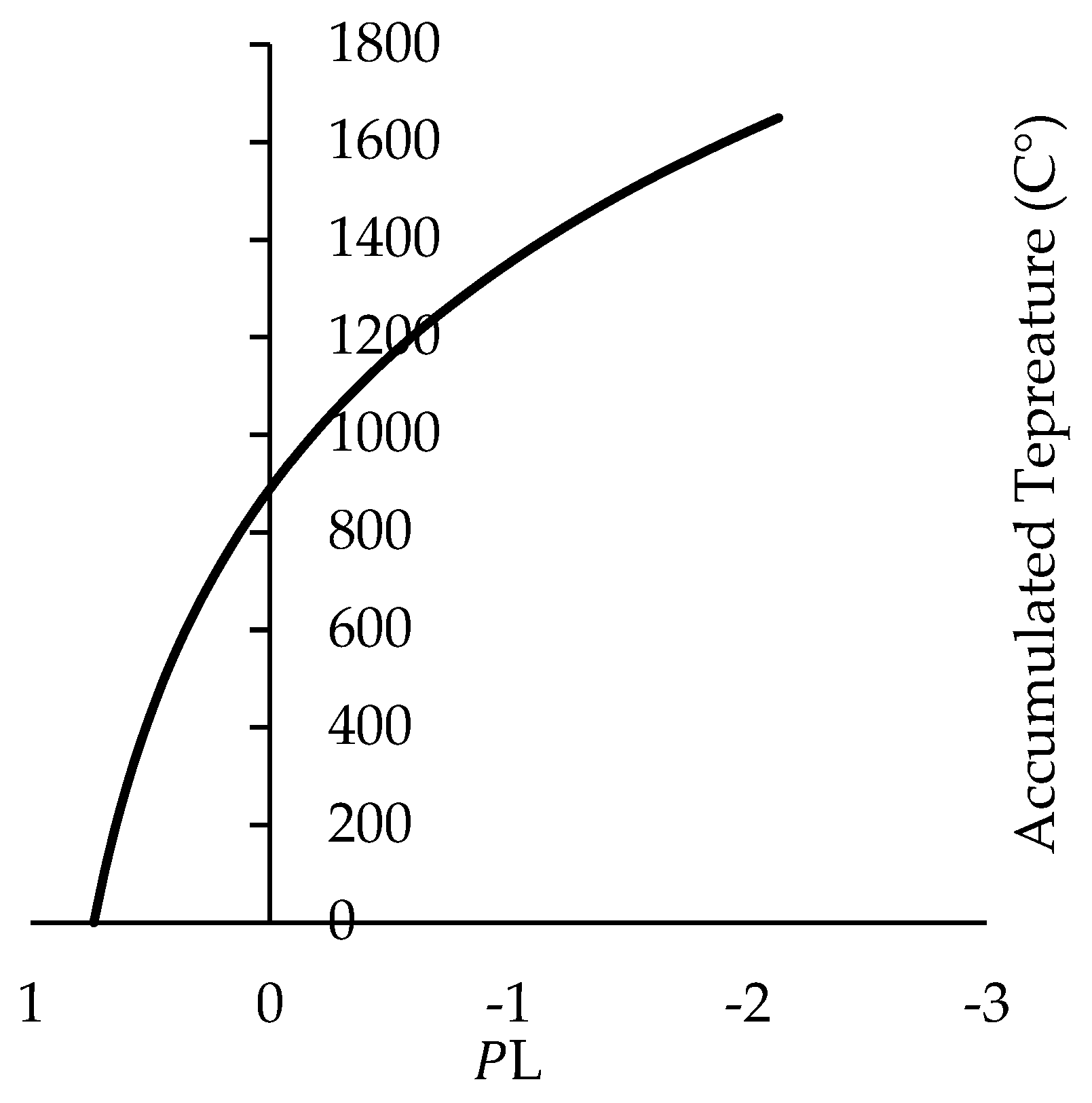
2.7. SAFY Model Calibration

The SAFY model has been used to estimate winter wheat DAM [34]. This model determines the optimized biomass production in the crop growing season based on the LUE [41] and leaf partitioning function [42] theories. Firstly, the daily DAM ( Δ D A M ) accumulation was calculated using the simple LUE theory with the equations shown below:
Δ D A M = E L U E × R g × ε C × f A P A R × F T ( T a )
f A P A R = 1 e k   × G L A I
where E L U E is the effective LUE, which is the LUE under environmental stress except temperature stress [36], R g is the incoming shortwave solar radiation, and ε C is the climate coefficient, which is the ratio of photosynthetically active radiation (PAR) to the shortwave solar radiation. In this study, the fixed value was adopted, ε C . = 0.48 [33,49,50], f A P A R is the fraction of absorbed photosynthetically active radiation; F T ( T a ) is the temperature stress, and the light-interception coefficient k is 0.5 under the assumption of the leaf angle distribution is uniform and the leaf inclination is a spherical distribution [44,51].
Secondly, the daily increase of GLAI ( Δ G L A I ) can be calculated from Δ D A M   which is portioned to leaves ( P L ) according to a given coefficient of specific leaf area ( S L A ). The equation given below:
Δ G L A I = Δ D A M × P L   ( T a ) × S L A
where the T a is the sum of optimal air temperature accumulated since plant emergence. P L   is the fraction between leaf and dry aboveground biomass, which is determined by air temperature and another two parameters (partition to leaf function parameters P L a   and P L b   ) [42]. The equation can be written as follows:
P L   ( T a ) = 1 P L a   × e P L b T a
After the air temperature reached the threshold S T T , the daily GLAI can be calculated from the following equation,
I f   T a > S T T
Δ G L A I = G L A I × ( T a S T T ) / R s
where R s is the rate of senescence.
After simulating the final DAM, the final crop yield can be calculated by multiplying the harvest index with the DAM. The harvest index ( H I ) was calculated from the ground biomass and final yield in S1, the average H I for all 12 sample points was 0.45. The yield can then be calculated using the equation below:
Y I E L D   = D A M   × H I

2.8. Winter Wheat Parameter Estimation from Ground-Based Biomass Measurement

The first step was attempted to determine the CSPs ( P L a , P L b , S T T , R s ) of winter wheat and the range of ELUE based on the experimental DAM data collected in S1. The CSPs depend on the genetic characteristics of the type and cultivar of the winter wheat. Five parameters affect the biomass partitioning which include two parameters P L a and P L b in the partition to leaf function P L (Equation (4)), the sum of temperature to start senescence S T T (°C), rate of senescence R s (°C/day), and ELUE is the ratio of photochemical energy produced as DAM from absorbed PAR (APAR).
Nine parameters identified in the literature, weather station measurements, and in-situ measurements (Table 2) were used to calibrate the SAFY model and determine the crop CSPs [34]. The nine parameters include (1) climatic efficiency ( ε C ), which is the ratio of PAR to the shortwave solar radiation; (2) minimum, optimal and maximum temperature ( T m i n , T o p t , and T m a x ) required for winter wheat growth; (3) specific leaf area ( S L A ), which is the unit weight of crop leave; (4) initial value of D A M at the day of plant emergence; (5) the light-interception coefficient ( k e x t ) in Bear’s law which is related to the plant leaf area index and the fraction of APAR; (6) the day of plant emergence; (7) the day of senescence; (8) the daily shortwave solar radiation ( R g ); and (9) daily mean air temperature ( T a ). Detailed values used in the SAFY model are given in Table 2. The five CSPs are calibrated in the first SAFY calibration.
The winter wheat CSPs and the range of ELUE were calibrated against the DAM observation collected in S1 using the global optimization method, Shuffled Complex Evolution-University of Arizona (SCE-UA) algorithm [52], to determine the optimal value for P L a , P L b , S T T , R s , and ELUE [5,34,36].
After running the optimization procedure using the SCE-UA algorithm (Duan, Sorooshian, & Gupta, 1994), the winter wheat CSPs and ELUE can be determined. The RMSE between the simulated DAM ( D A M s i m ) and the In-situ true DAM ( D A M t r u e ) was used as the cost function of the calibration:
R M S E D A M = [ 1 N i = 1 N ( D A M s i m D A M t r u e ) 2 ] 1 2
Model calibration was performed by minimizing the RMSE between DAMsim and DAMtrue. In the SAFY model, the optimization procedure was run 10,000 times for each sampling location to achieve the optimal parameters with the lowest RMSE. In addition, RRMSE was also used to indicate model accuracy.
R R M S E D A M = R M S E D A M i = 1 N D A M t r u e × 100 %

2.9. Fisheye-Derived GLAI and Model-Simulated GLAI

As the first calibration generated the daily GLAI values for 12 sampling locations for the entire growing season using the SAFY model, these GLAI values can be used to calibrate the fisheye derived LAIe. The relationship between the fisheye LAIe and the GLAI was established using the data from S1. This relationship was then used to convert the fisheye derived LAIe in S2 and used as input for the SAFY model to simulate the DAM and SAFY-GLAY in S2. A second calibration of the SAFY model was performed for S2 using the winter wheat CSPs ( P L a , P L b , S T T , R s ), and the GLAI which is converted from fisheye-derived LAIe measurements in S2 to simulate the SAFY-GLAI and final DAM. The median values of these CSPs were then adopted and the ELUE was kept as a variable in the second calibration. The RMSE between the simulated GLAI ( G L A I s i m ) and the converted fisheye LAI measurements ( G L A I t r u e ) were used as the cost function in the SCE-UA algorithm during the calibration.
R M S E G L A I = [ 1 N i = 1 N ( G L A I s i m G L A I t r u e ) 2 ] 1 2
The calibration procedure was also performed 10,000 times to ensure the optimal GLAI simulation with the lowest RMSE.

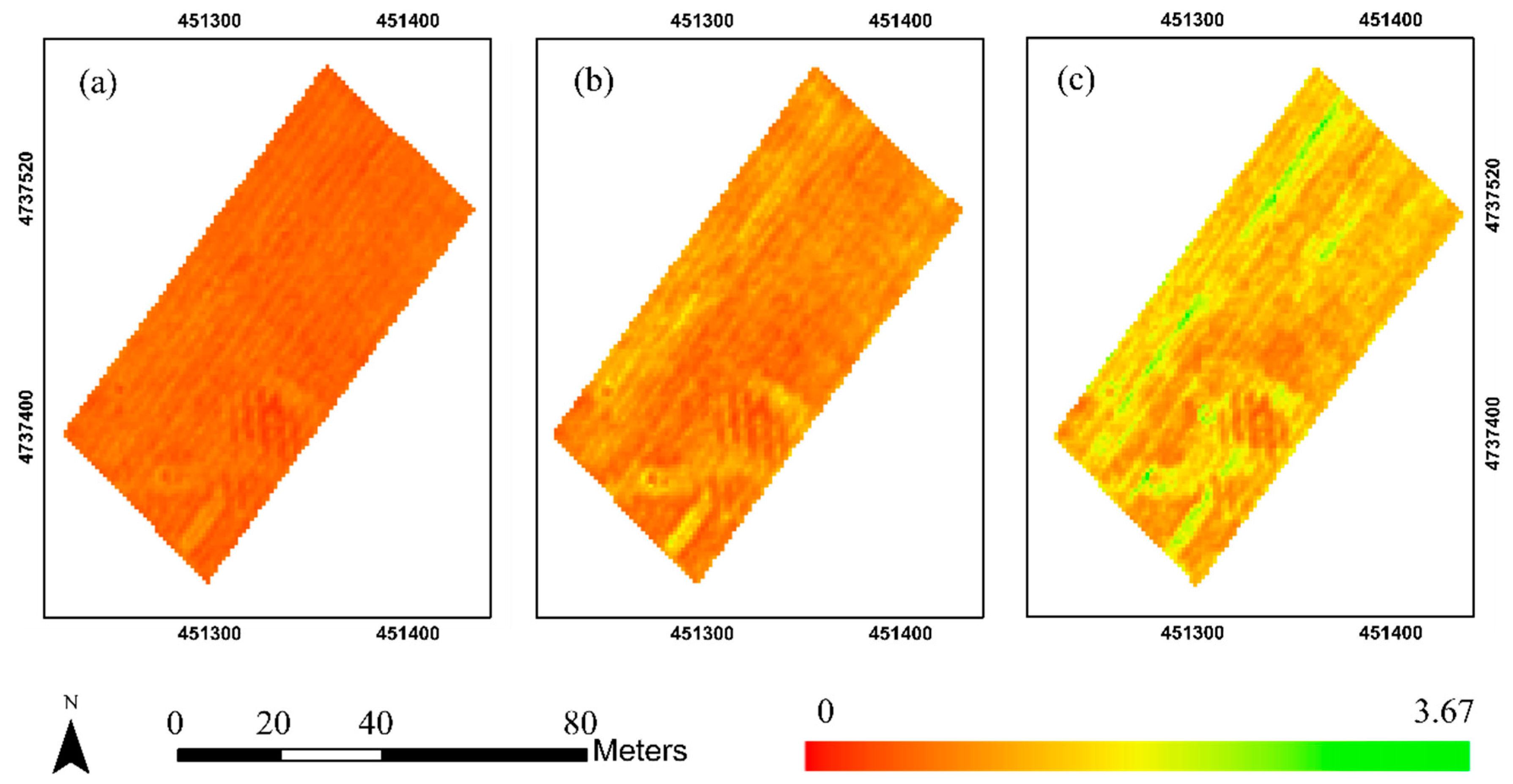
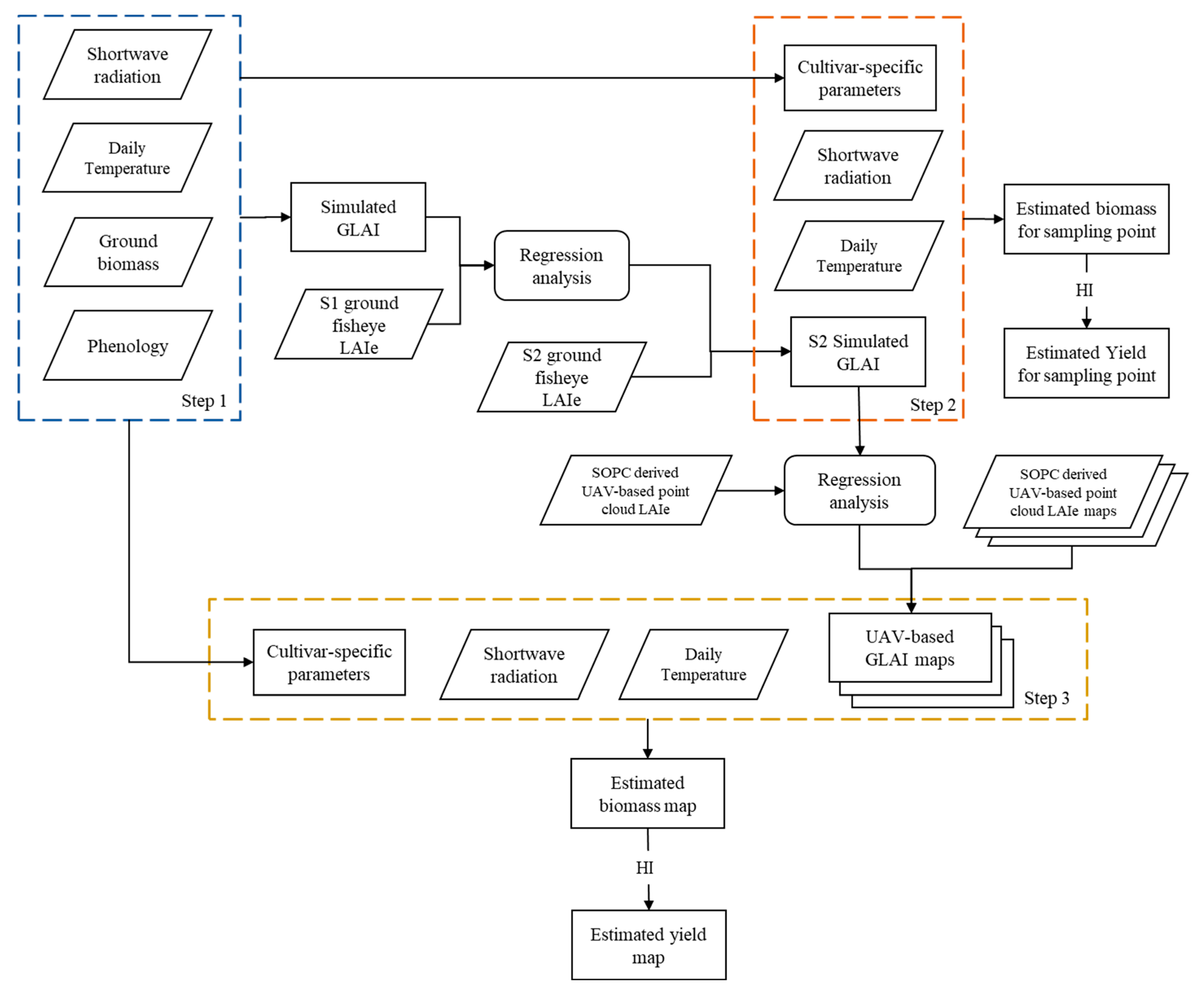
2.10. Final DAM and Yield Estimation Using UAV-Based LAIe in S2

The relationship between the UAV-based LAIe and simulated SAFY-GLAI derived from the second SAFY calibration was then established from the second calibration. After converting the UAV-based LAIe to GLAI, the third SAFY calibration was performed for S2 using the winter wheat CSPs derived from the first SAFY calibration and the UAV-based GLAI to simulate the DAM in S2. The total of UAV-based LAIe has 5977 measurements for S2 on each monitoring date. The final DAM was estimated by optimizing the lowest RMSE of GLAI value using Equation (9). The final yield was calculated using Equation (6). After resampling the UAV-based final yield to the same resolution of the harvester yield data, the mean, standard deviation, and coefficient of variation (CV) were used to evaluate the performance of yield estimation. The flow chart below illustrates the steps of winter wheat yield estimation using the UAV-based LAI (Figure 6).

3. Results

3.1. Determination of Cultivar-Specific Parameters

After the initial SAFY model calibration using the In-situ DAM, the ranges of P L a , P L b , S T T , R s and ELUE were determined. Table 3 shows the results of the five parameters, including maximum, minimum, median, mean, and standard deviation (STD). The median value of P L a , P L b , S T T , and R s were adopted from the second and third SAFY model calibration [34]. The RMSE between the In-situ DAM measurements and simulated DAM in S1 was 81 g/m2, and the RRMSE is 13.89%.

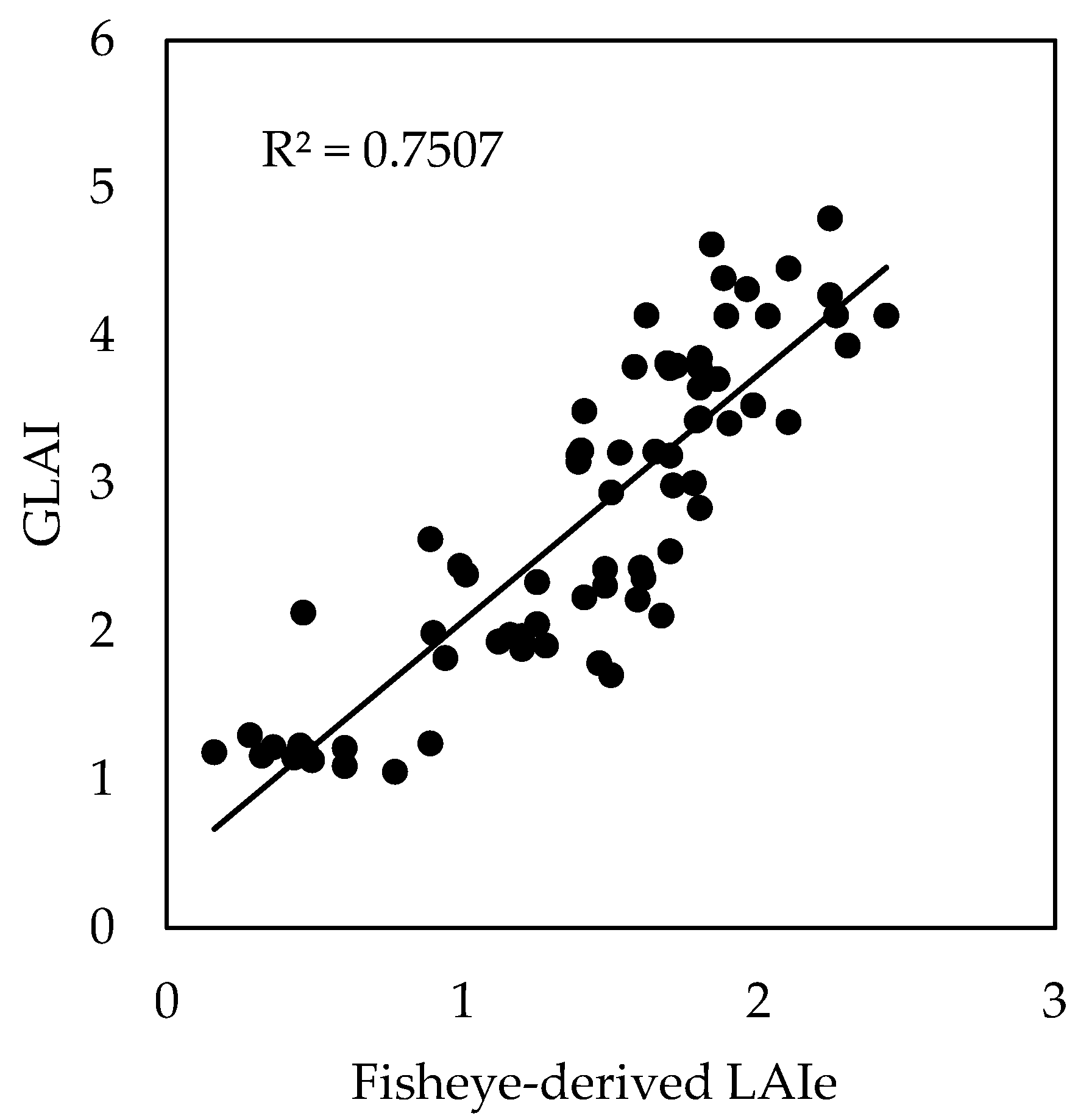
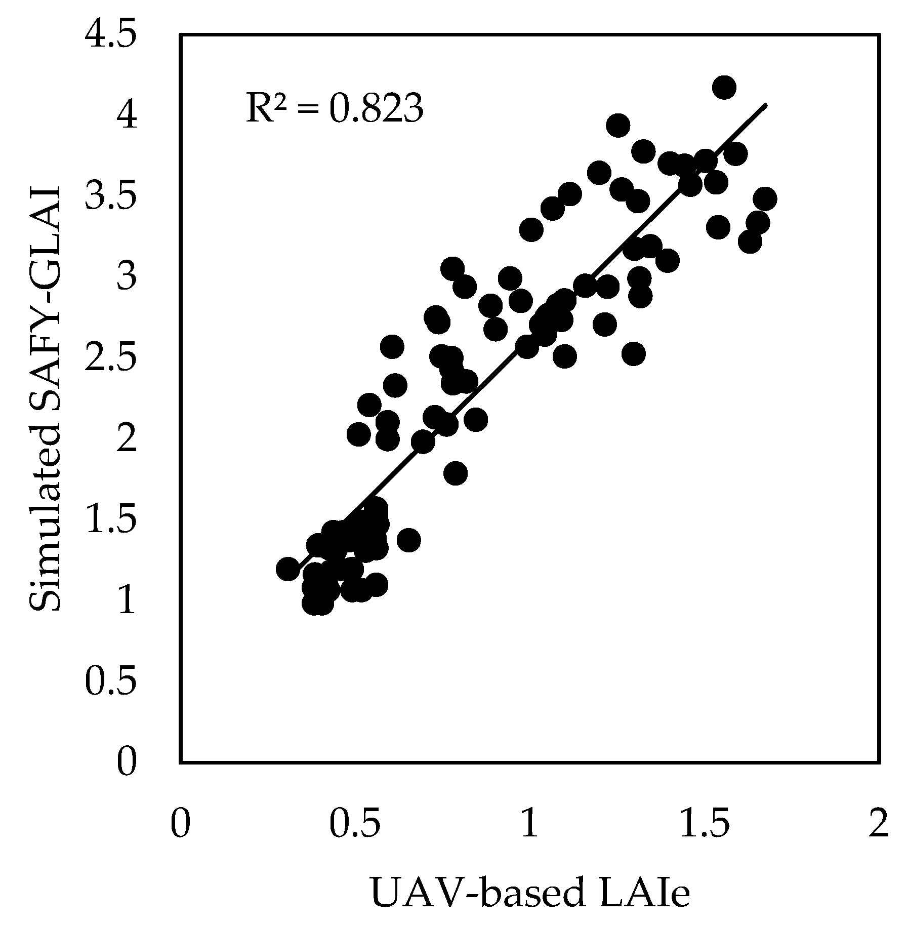
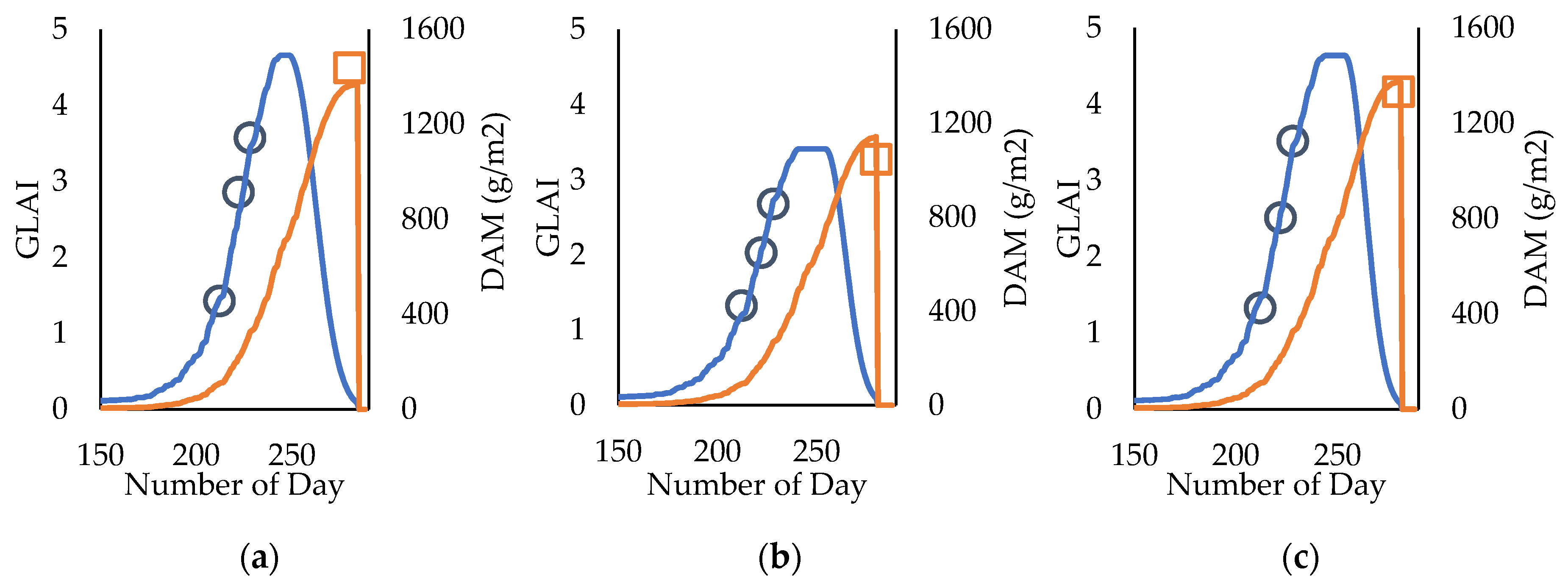
3.2. Relationship between Simulated SAFY-GLAI and Fisheye-Derived LAIe in S1 and S2

After the first SAFY calibration (Figure 6, step 1), the simulated daily SAFY-GLAI were generated from DAM calibration for 12 sampling locations in S1, and the relationship between the simulated GLAI and fisheye-derived LAIe were established (Figure 7). The coefficient of determination (R2) was 0.75 for all 60 measurements.
Using this relationship between fisheye-derived LAIe and simulated GLAI in S1, the fisheye-derived LAIe measurements in S2 were converted to simulated GLAI. The second SAFY model calibration (Figure 6, step 2) was conducted using the simulated GLAI values of 32 sampling locations in S2, the final DAM and simulated daily SAFY-GLAI of these locations was determined in the second SAFY calibration. After estimating the final DAM for the 32 sampling locations in S2 from the second calibration, the In-situ measured final DAM and simulate DAM derived from SAFY model were compared (Figure 8). The R2 between the estimation and measured grain yield was 0.48, the RMSE was 54 g/m2, and the RRMSE was 9.37%.

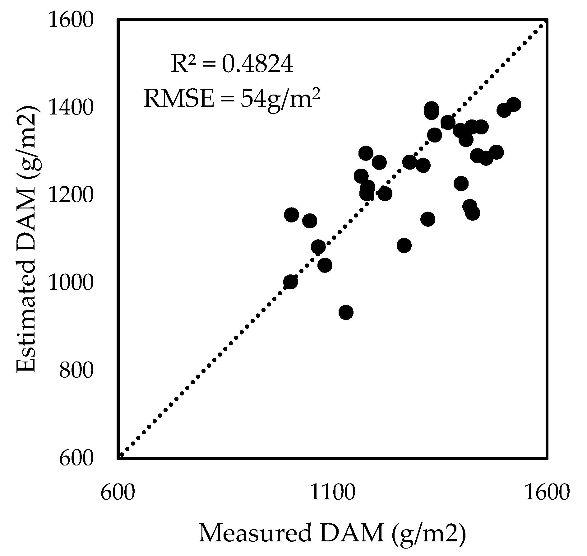
3.3. DAM Estimation Using UAV-Based LAIe Measurements

After the second calibration of SAFY model in S2, the simulated daily SAFY-GLAI were generated from the GLAI (converted from fisheye-LAIe) for 32 sampling locations. By comparing the results of simulated SAFY-GLAI and the SOPC derived UAV-based LAIe of 32 sampling location, the relationship between the simulated SAFY-GLAI and UAV-based LAIe was established for three monitoring days and shown in Figure 9. The R2 was 0.82 for all 96 measurements. Based on this relationship, the multiple UAV-based LAIe maps will be converted to GLAI maps. These GLAI maps will be used in the third SAFY calibration (Figure 6, step 3) to estimate the final DAM in S2.
Figure 10 depicts the converted UAV-derived LAIe, the daily simulated SAFY-GLAI, the daily simulated DAM, and the final DAM value derived from the second SAFY model calibration for point 8 (Figure 10a), 16 (Figure 10b), and 26 (Figure 10c) of S2. The final DAM map was generated with the same spatial resolution as the UAV-based LAIe map. Figure 11 shows the final DAM maps at the resolution at 2 × 2 m.

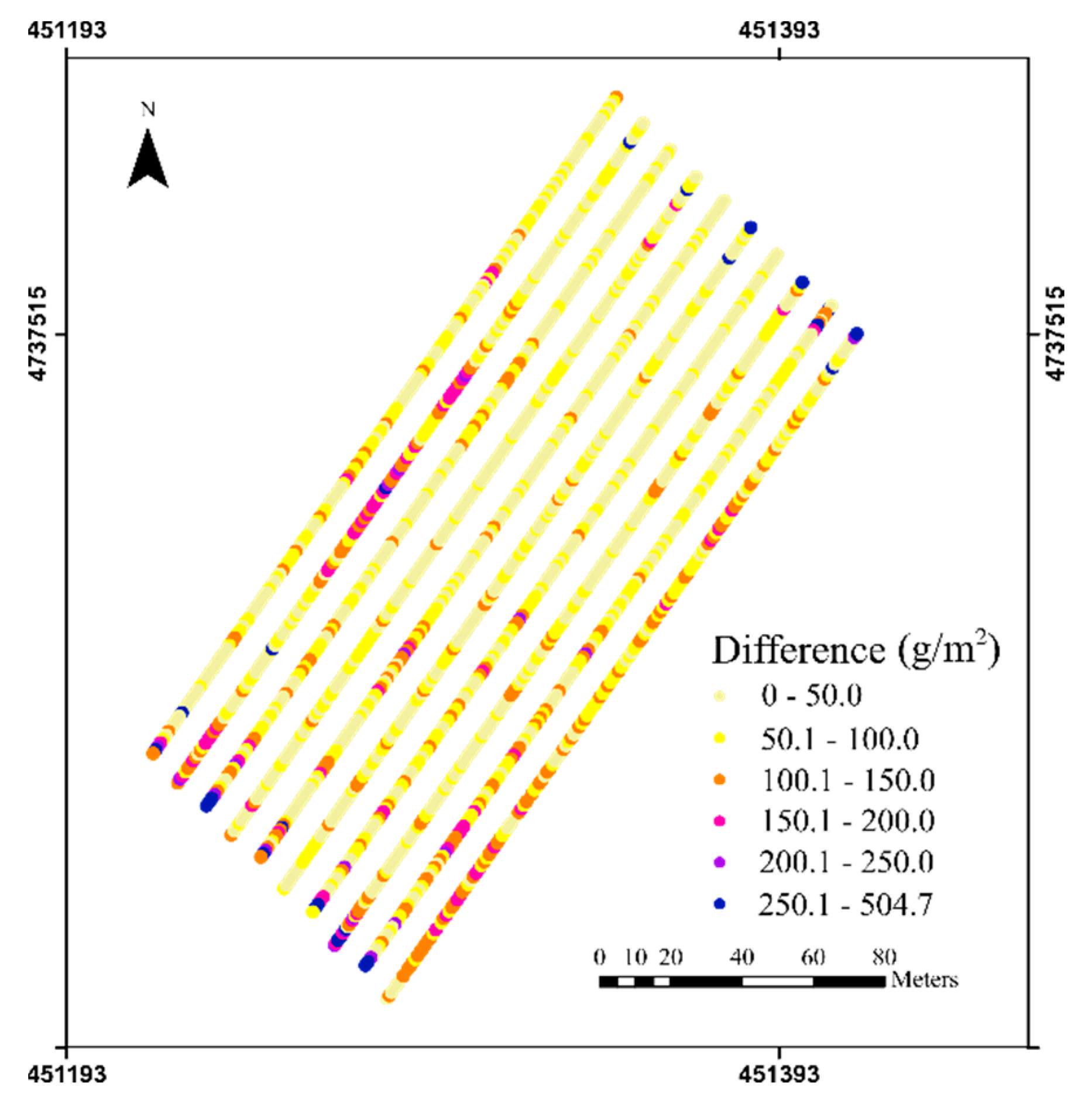
3.4. Comparison of True Grain Yield and Estimated Yield

Table 4 shows statistical information of the harvester and estimated yield maps. Figure 12 shows the maps of harvester measured grain yield (Figure 12a) and estimated yield (Figure 12b) for S2. The accuracy of the estimated yield was evaluated by comparing their RMSE, mean, standard deviation (STD), and CV. Figure 13 shows the absolute difference map between true grain yield and estimated yield for S2.

4. Discussion

4.1. Cultivar-Specific Parameters Derived from the First SAFY Model Calibration

The determination of the CSPs ( P L a , P L b , S T T , R s and ELUE) can help the SAFY model in crop final biomass estimation. Many studies have provided the ranges of these parameters. For instance, Duchenmin et al. (2008) determined the range of P L a and P L b for winter wheat as 0.05–0.5 and 10−5–10−2 respectively. The median values of P L a = 0.1573 and P L b = 0.00196 were adopted during the final DAM estimation. In this study, the ranges of P L a and P L b used were 0.2038–0.2686 and 0.0015–0.0021, respectively. The ranges of the two parameters used in our study are much smaller in comparison with that of in the literature. This is because the In-situ DAM measurements were used to calibrate the SAFY model and the day of plant emergence was observed through In-situ observation. The P L a and P L b combined with the accumulated temperature will affect the value of P L (Equation (4)). Figure 14 shows the relationship between P L and the accumulated temperature in this study. The P L decreases exponentially from the value of 1 to the value of 0 with the accumulated temperature, which is the plant emergence to the end of the leave production phase [42]. The P L is the ratio of the daily increase of GLAI and the daily increase of DAM, the value of 0 marks the stopping point of leave developments. As illustrated in Figure 14, P L is zero when the accumulated temperature is at 881 °C, and the date was 14 June. According to in-situ observation on 16 June, winter wheat was at the end of flowering stage at that time.
The simulated total accumulated temperature ( S T T ) determined by SAFY was 954 °C when senescence started. The date for achieving this temperature was 17 June, which was one day later than winter wheat flowering stage. According to the relationship between phenology and total accumulated temperature, the winter wheat starts seed fill at this temperature [54]. Beyond this threshold temperature, the GLAI calculated using Equation (5) started to decrease. In Equation (5), the R s is related to the threshold temperature and total accumulated temperature for maturity. The total accumulated temperature can be used to determine the date of maturity with the aid of the weather data. Based on the value of S T T and R s , the total accumulated temperature for maturity of all 12 samples were evaluated using the SAFY model for S1. The average total mature day is 282, which is five days earlier than the day of harvest (287). The values of the sum of temperature for senescence ( S T T ) and the rate of senescence ( R s ) are consistent with the actual in-situ observations.

4.2. ELUE

ELUE plays an important role in the SAFY model. ELUE is largely influenced by crop species, physiological factors, soil conditions, and weather conditions. Soil conditions such as soil nutrient, soil moisture, texture, organic matter, and pH vary across the field and can lead to variable ELUE values for the same crop. Conventionally, a constant ELUE value is used for the entire field in yield estimation. Dong et al. (2017) introduced the spatially variable crop maximum LUE for the first time and achieved significant improvements in biomass estimation accuracy for winter wheat and corn. Liao et al. (2019) also used variable ELUE values to estimate the yield of corn and soybean. Therefore, in this study the ELUE was adopted as a variable parameter in the SAFY model rather than a fixed value as the P L a , P L b , S T T , and R s in the second and third calibrations. The range of ELUE in the first calibration was 2.93–3.18, which fits in the range of ELUE in the literature [5,34].

4.3. Uncertainties of the Estimated Crop Biomass and Yield

By comparing the yield maps in Figure 12, both the estimated and measured maps have similar patterns at the bottom corner, but the upper left area in the field has different yield estimations. Figure 13 shows the absolute difference between the true grain yield and estimated yield for S2. Since the disease and pests stress were not observed during the fieldwork in the winter wheat field. The absolute difference in the upper left area in the field may be affected by some external factors such as soil water content and nutrient. Because the SAFY model simplifies the crop growth model which considers the temperature stress only, the soil water and nutrient stress after the last LAI monitoring may lead to an inaccurate final DAM estimation. Except the upper left area, most of the test points have small differences which are less than 100 g/m2. Some test points with large yield differences are located at the end of rows which may cause by the basis of the harvester. Because the harvester needs to lift the head during turning. The uncertainties of the yield estimation on the upper left area might have been due to the limited number of UAV-based LAIe maps. The early LAIe measurements of the winter wheat were used in the SAFY model to estimate the final DAM and yield. The last UAV-based LAIe measurement was 50 days earlier than the actual harvest date. The LAIe information used only captured the crop growth condition up to the date of the last UAV flight which could not have taken into condition of the further biomass growth during the later season. The multiple data sources can be considered to increase the temporal resolution of the GLAI for the SAFY model.
The histograms of the UAV-based yield and the harvester measured yield map are shown in Figure 15. Overall, these two yield histograms exhibit a similar distribution, in which the range of harvester measured yield data was between 340 to 840 g/m2, and the range of the estimate yield data was between 420 to 780 g/m2. The UAV estimated yield has a lower standard deviation and CV than that of the harvester measured yield data in S2. This is likely due to the fixed P L a and P L b used in the SAFY model. In addition, the ground-based yield map, generated by the combine harvester, might have suffered yield loss in comparison with manual harvest. The destructive biomass is more accurate in estimating GLAI and yield during the SAFY model calibrations. This may be one of the reasons for the difference between the true and estimate yield maps. Due to the use of destructive biomass, the estimated yield has a slightly narrower histogram distribution in the yield map. In addition, the final yield might have been influenced by the fixed harvest index. The UAV-based yield was calculated from the average harvest index derived from 12 sampling points. However, the crop growth condition can influence the harvest index and lead to a different yield estimation [55].

4.4. Application and Contribution

This study, for the first time, applied the SOPC derived UAV-based point cloud LAIe maps to the SAFY model to generate the sub-field biomass and yield maps. It is also the first time to use the UAV-based data to the SAFY model. One of the potential applications of this framework is for yield estimation. This can help reveal the spatial variability of yield potential for winter wheat at the sub-field scale. The LAI maps generated at various growth stages can also provide useful information to assist in making crop management decisions. The soft red winter wheat CSPs determined in this study can be used in future studies for the same region. Since this framework is designed for UAV application at farm level, the day of planting and emergence can be obtained from in-situ observation. With specific phenological date and the CSPs, yield prediction using the SAFY model and the UAV derived simulated GLAI only requires the solar radiation and temperature data. Therefore, it is possible to predict the winter wheat final yield using weather data collected at real-time and simulated for the rest of the growing season using the proposed framework.
The normalization of LAIe derived from different platforms can help the SAFY model application to final DAM estimation using different data sources. The normalization approach can be applied to other crops to determine the CSPs. In this study, the normalized UAV-based point cloud LAIe were used in the SAFY model calibration for final DAM and yield estimation. The UAV-based point cloud LAIe can provide a variable range of spatial resolution map from submeter to meter scale (50 cm to 5 m) which can clearly display the within-field final DAM and yield variability.
Fu et al. (2020) [45] estimated the winter wheat biomass using the UAV-based multispectral imagery. The RRMSE of the DAM were 23.37%. In this study, the DAM values were estimated from only 30 individual sampling locations. In contrast, this study achieved a RRMSE of 15% for more than 1800 points. In addition, this study uses the UAV-based PCD derived from RGB imagery instead of multispectral vegetation indices. The SOPC method does not require any ground spectral calibration, which is more accessible and low cost. The final DAM and yield estimation could be conducted without ground measurements in this study. Furthermore, the method of this study could be applied on different geographical locations and other crops. The solar radiation and air temperature should be collected for the different locations. The SOPC-LAIe calculates the crop leaf area index based on the gap fraction theory under the assumption of the leaf angle distribution is uniform and the leaf inclination follows spherical distribution [44,51]. If the crop leaf area index can be calculated using the gap fraction theory with the same assumption. This method is practical for different locations and crops. For example, the gap fraction theory on leaf area index estimation and the SAFY model on yield estimation have been proved on corn and soybean [36]. This method may possible be applied on corn and soybean and to estimate the final yield.

5. Conclusions

In this study, destructive biomass was used to calibrate the SAFY model to derive CSPs for winter wheat instead of using the LAI measurements to calibrate the SAFY model for determining of CPSs. Through the normalization of the SOPC-LAIe maps to the simulated SAFY-GLAI maps, the UAV-based point cloud derived LAIe can be used as input to the SAFY model for winter wheat final DAM and yield estimation. This is the first time the SOPC derived LAIe was used for final DAM and yield estimation of winter wheat. It is also the first time to apply the UAV-based LAI to the SAFY model to estimate the final DAM. The results showed that the SOPC method derived UAV-based point-cloud LAIe and the SAFY model have a great potential in generating high-spatial resolution (2 × 2 m in this study) DAM and yield map. The final yield estimation achieved the RMSE of 88 g/m2 and RRMSE of 15.22%. The UAV-based point cloud derived LAIe before the booting stages can be used to estimate the final DAM and yield of winter wheat. The CSPs determination approach developed in this study can be adopted in deriving crop CSPs for other crop types when using SAFY model to estimate and forecast final DAM and grain yield. After determining the CSPs of crops, the approach can be achieved without having to rely on ground measurements, which is a great advantage for operational near-real-time operations.
Given the success of the reported results, this stud still has the limitations. For future work, UAV imagery collected at the late growth stages can be incorporated into the analysis to achieve improved estimation accuracy. In addition, more detailed soil information, such as moisture content, nutrient level, and soil organic matter, should also be used as model input to improved model performance.

Author Contributions

Conceptualization, Y.S.; Methodology, Y.S.; writing-original draft preparation, Y.S.; writing-review and editing, Y.S., J.W., J.S., C.L.; supervision, J.W.; funding acquisition, Y.S., J.W. All authors have read and agreed to the published version of the manuscript.

Funding

This work is partially funded by NSERC discovering Grant awarded to Wang; a MITACS accelerate internship sponsored by MITACS and A&L Canada Laboratories Inc., and an NSERC CRD grant awarded to Leblon, Wang and Sabarinathan.

Acknowledgments

We would like to thank Minfeng Xing, Qinghua Xie, Huang Lee, Jody Yu, and Dandan Wang for their helpful work on field data collection. We also thank A&L Laboratories Inc. provided the study field.

Conflicts of Interest

The authors declare no conflict of interest.

References

  1. Schimmelpfennig, D. Farm Profits and Adoption of Precision Agriculture; (Economic Research Report, 217); United States Department of Agriculture: Washington, DC, USA, 2016.
  2. Idso, S.B.; Jackson, R.D.; Reginato, R.J. Remote-sensing of crop yields. Science 1977, 196, 19–25. [Google Scholar] [CrossRef] [PubMed]
  3. Liu, J.; Miller, J.R.; Pattey, E.; Haboudane, D.; Strachan, I.B.; Hinther, M. Monitoring crop biomass accumulation using multi-temporal hyperspectral remote sensing data. Int. Geosci. Remote Sens. Symp. (IGARSS) 2004, 3, 1637–1640. [Google Scholar] [CrossRef]
  4. Toscano, P.; Castrignanò, A.; Di Gennaro, S.F.; Vonella, A.V.; Ventrella, D.; Matese, A. A precision agriculture approach for durum wheat yield assessment using remote sensing data and yield mapping. Agronomy 2019, 9, 437. [Google Scholar] [CrossRef] [Green Version]
  5. Dong, T.; Liu, J.; Qian, B.; Zhao, T.; Jing, Q.; Geng, X.; Wang, J.; Huffman, T.; Shang, J. Estimating winter wheat biomass by assimilating leaf area index derived from fusion of Landsat-8 and MODIS data. Int. J. Appl. Earth Obs. Geoinf. 2016, 49, 63–74. [Google Scholar] [CrossRef]
  6. Dong, T.; Shang, J.; Liu, J.; Qian, B.; Jing, Q.; Ma, B.; Huffman, T.; Geng, X.; Sow, A.; Shi, Y.; et al. Using RapidEye imagery to identify within-field variability of crop growth and yield in Ontario, Canada. Precis. Agric. 2019, 20, 1231–1250. [Google Scholar] [CrossRef]
  7. Shang, J.; Liu, J.; Ma, B.; Zhao, T.; Jiao, X.; Geng, X.; Huffman, T.; Kovacs, J.M.; Walters, D. Mapping spatial variability of crop growth conditions using RapidEye data in Northern Ontario, Canada. Remote Sens. Environ. 2015, 168, 113–125. [Google Scholar] [CrossRef]
  8. Rudorff, A.F.; Batista, G.T. Wheat yield estimation at the farm level using tm landsat and agrometeorological data. Int. J. Remote Sens. 1991, 12, 2477–2484. [Google Scholar] [CrossRef]
  9. Ruwaimana, M.; Satyanarayana, B.; Otero, V.M.; Muslim, A.; Syafiq, A.M.; Ibrahim, S.; Raymaekers, D.; Koedam, N.; Dahdouh-Guebas, F. The advantages of using drones over space-borne imagery in the mapping of mangrove forests. PLoS ONE 2018, 13, e0200288. [Google Scholar] [CrossRef] [PubMed] [Green Version]
  10. Song, Y.; Wang, J. Winter wheat canopy height extraction from UAV-based point cloud data with a moving cuboid filter. Remote Sens. 2019, 11, 1239. [Google Scholar] [CrossRef] [Green Version]
  11. Duan, B.; Fang, S.; Zhu, R.; Wu, X.; Wang, S.; Gong, Y.; Peng, Y. Remote estimation of rice yield with unmanned aerial vehicle (uav) data and spectral mixture analysis. Front. Plant Sci. 2019, 10, 1–14. [Google Scholar] [CrossRef] [Green Version]
  12. Sanches, G.M.; Duft, D.G.; Kölln, O.T.; Luciano, A.C.D.S.; De Castro, S.G.Q.; Okuno, F.M.; Franco, H.C.J. The potential for RGB images obtained using unmanned aerial vehicle to assess and predict yield in sugarcane fields. Int. J. Remote Sens. 2018, 39, 5402–5414. [Google Scholar] [CrossRef]
  13. Bansod, B.; Singh, R.; Thakur, R.; Singhal, G. A comparision between satellite based and drone based remote sensing technology to achieve sustainable development: A review. J. Agric. Environ. Int. Dev. 2017, 111, 383–407. [Google Scholar] [CrossRef]
  14. Zhang, C.; Kovacs, J.M. The application of small unmanned aerial systems for precision agriculture: A review. Precis. Agric. 2012, 13, 693–712. [Google Scholar] [CrossRef]
  15. Yao, X.; Wang, N.; Liu, Y.; Cheng, T.; Tian, Y.; Chen, Q.; Zhu, Y. Estimation of wheat LAI at middle to high levels using unmanned aerial vehicle narrowband multispectral imagery. Remote Sens. 2017, 9, 1304. [Google Scholar] [CrossRef] [Green Version]
  16. Hoffmann, H.; Jensen, R.; Thomsen, A.; Nieto, H.; Rasmussen, J.; Friborg, T. Crop water stress maps for entire growing seasons from visible and thermal UAV imagery. Biogeosciences 2016, 1–30. [Google Scholar] [CrossRef] [Green Version]
  17. Huang, Y.; Reddy, K.N.; Fletcher, R.S.; Pennington, D. UAV Low-Altitude Remote Sensing for Precision Weed Management. Weed Technol. 2018, 32, 2–6. [Google Scholar] [CrossRef]
  18. Schirrmann, M.; Hamdorf, A.; Garz, A.; Ustyuzhanin, A.; Dammer, K. Estimating wheat biomass by combining image clustering with crop height. Comput. Electron. Agric. 2016, 121, 374–384. [Google Scholar] [CrossRef]
  19. Berni, J.; Zarco-Tejada, P.J.; Suarez, L.; Fereres, E. Thermal and Narrowband Multispectral Remote Sensing for Vegetation Monitoring from an Unmanned Aerial Vehicle. IEEE Trans. Geosci. Remote Sens. 2009, 47, 722–738. [Google Scholar] [CrossRef] [Green Version]
  20. Dong, T.; Liu, J.; Qian, B.; Jing, Q.; Croft, H.; Chen, J.; Wang, J.; Huffman, T.; Shang, J.; Chen, P. Deriving Maximum Light Use Efficiency from Crop Growth Model and Satellite Data to Improve Crop Biomass Estimation. IEEE J. Sel. Top. Appl. Earth Obs. Remote Sens. 2017, 10, 104–117. [Google Scholar] [CrossRef]
  21. Casanova, D.; Epema, G.F.; Goudriaan, J. Monitoring rice reflectance at field level for estimating biomass and LAI. Field Crop. Res. 1998, 55, 83–92. [Google Scholar] [CrossRef]
  22. Idso, S.B.; Pinter, P.J.; Jackson, R.D.; Reginato, R.J. Estimation of grain yields by remote sensing of crop senescence rates. Remote Sens. Environ. 1980, 9, 87–91. [Google Scholar] [CrossRef]
  23. Hunt, E.R.; Dean Hively, W.; Fujikawa, S.J.; Linden, D.S.; Daughtry, C.S.T.; McCarty, G.W. Acquisition of NIR-green-blue digital photographs from unmanned aircraft for crop monitoring. Remote Sens. 2010, 2, 290–305. [Google Scholar] [CrossRef] [Green Version]
  24. Hoefsloot, P.; Ines, A.; Van Dam, J.; Duveiller, G.; Kayitakire, F.; Hansen, J. Combining Crop Models and Remote Sensing for Yield Prediction: Concepts, Applications and Challenges for Heterogeneous Smallholder Environments; European Union: Luxembourg, 2012; ISBN 978-92-79-27883-9. [Google Scholar]
  25. Shang, J.; Liu, J.; Huffman, T.; Qian, B.; Pattey, E.; Wang, J.; Zhao, T.; Geng, X.; Kroetsch, D.; Dong, T.; et al. Estimating plant area index for monitoring crop growth dynamics using Landsat-8 and RapidEye images. J. Appl. Remote Sens. 2014, 8, 085196. [Google Scholar] [CrossRef] [Green Version]
  26. Kouadio, L.; Newlands, N.K.; Davidson, A.; Zhang, Y.; Chipanshi, A. Assessing the performance of MODIS NDVI and EVI for seasonal crop yield forecasting at the ecodistrict scale. Remote Sens. 2014, 6, 10193–10214. [Google Scholar] [CrossRef] [Green Version]
  27. Zhou, X.; Zheng, H.B.; Xu, X.Q.; He, J.Y.; Ge, X.K.; Yao, X.; Cheng, T.; Zhu, Y.; Cao, W.X.; Tian, Y.C. Predicting grain yield in rice using multi-temporal vegetation indices from UAV-based multispectral and digital imagery. ISPRS J. Photogramm. Remote Sens. 2017, 130, 246–255. [Google Scholar] [CrossRef]
  28. Khaki, S.; Wang, L. Crop yield prediction using deep neural networks. Front. Plant Sci. 2019, 10, 1–10. [Google Scholar] [CrossRef] [Green Version]
  29. Kim, N.; Ha, K.J.; Park, N.W.; Cho, J.; Hong, S.; Lee, Y.W. A comparison between major artificial intelligence models for crop yield prediction: Case study of the midwestern United States, 2006–2015. Int. J. Geo-Inf. 2019, 8, 240. [Google Scholar] [CrossRef] [Green Version]
  30. Cheng, Z.; Meng, J.; Wang, Y. Improving spring maize yield estimation at field scale by assimilating time-series HJ-1 CCD data into the WOFOST model using a new method with fast algorithms. Remote Sens. 2016, 8, 303. [Google Scholar] [CrossRef] [Green Version]
  31. Kuwata, K.; Shibasaki, R. Estimating Corn Yield in the United States with Modis Evi and Machine Learning Methods. ISPRS Ann. Photogramm. Remote Sens. Spat. Inf. Sci. 2016, 8, 131–136. [Google Scholar] [CrossRef]
  32. Yue, J.; Yang, G.; Tian, Q.; Feng, H.; Xu, K.; Zhou, C. Estimate of winter-wheat above-ground biomass based on UAV ultrahigh-ground-resolution image textures and vegetation indices. ISPRS J. Photogramm. Remote Sensi. 2019, 150, 226–244. [Google Scholar] [CrossRef]
  33. Brisson, N.; Gary, C.; Justes, E.; Roche, R.; Mary, B.; Ripoche, D.; Zimmer, D.; Sierra, J.; Bertuzzi, P.; Burger, P.; et al. An overview of the crop model STICS. Eur. J. Agron. 2003, 18, 309–332. [Google Scholar] [CrossRef]
  34. Duchemin, B.; Maisongrande, P.; Boulet, G.; Benhadj, I. A simple algorithm for yield estimates: Evaluation for semi-arid irrigated winter wheat monitored with green leaf area index. Environ. Model. Softw. 2008, 23, 876–892. [Google Scholar] [CrossRef] [Green Version]
  35. Lobell, D.B.; Asseng, S. Comparing estimates of climate change impacts from process-based and statistical crop models. Environ. Res. Lett. 2017, 12, 1–12. [Google Scholar] [CrossRef]
  36. Liao, C.; Wang, J.; Dong, T.; Shang, J.; Liu, J.; Song, Y. Using spatio-temporal fusion of Landsat-8 and MODIS data to derive phenology, biomass and yield estimates for corn and soybean. Sci. Total Environ. 2019, 650, 1707–1721. [Google Scholar] [CrossRef] [PubMed]
  37. Liu, J.; Shang, J.; Qian, B.; Huffman, T.; Zhang, Y.; Dong, T.; Jing, Q.; Martin, T. Crop yield estimation using time-series MODIS data and the effects of cropland masks in Ontario, Canada. Remote Sens. 2019, 11, 2419. [Google Scholar] [CrossRef] [Green Version]
  38. Steduto, P.; Hsiao, T.C.; Raes, D.; Fereres, E. Aquacrop-the FAO crop model to simulate yield response to water: I. concepts and underlying principles. Agron. J. 2009, 101, 426–437. [Google Scholar] [CrossRef] [Green Version]
  39. van Diepen, C.A.; Wolf, J.; van Keulen, H.; Rappoldt, C. WOFOST: A simulation model of crop production. Soil Use Manag. 1989, 5, 16–24. [Google Scholar] [CrossRef]
  40. Silvestro, P.C.; Pignatti, S.; Pascucci, S.; Yang, H.; Li, Z.; Yang, G.; Huang, W.; Casa, R. Estimating wheat yield in China at the field and district scale from the assimilation of satellite data into the Aquacrop and simple algorithm for yield (SAFY) models. Remote Sens. 2017, 9, 509. [Google Scholar] [CrossRef] [Green Version]
  41. Monteith, J.L. Solar radiation and productivity in tropical ecosystems. J. Appl. Ecol. 1972, 9, 747–766. [Google Scholar] [CrossRef] [Green Version]
  42. Maas, S.J. Parameterized Model of Gramineous Crop Growth: I. Leaf Area and Dry Mass Simulation. Agron. J. 1993, 85, 348. [Google Scholar] [CrossRef]
  43. Zhang, C.; Liu, J.; Dong, T.; Shang, J.; Tang, M.; Zhao, L.; Cai, H. Evaluation of the simple algorithm for yield estimate model in winter wheat simulation under different irrigation scenarios. Agron. J. 2019, 111, 2970–2980. [Google Scholar] [CrossRef]
  44. Zheng, G.; Moskal, L.M. Retrieving Leaf Area Index (LAI) Using Remote Sensing: Theories, Methods and Sensors. Sensors 2009, 9, 2719–2745. [Google Scholar] [CrossRef] [PubMed] [Green Version]
  45. Fu, Z.; Jiang, J.; Gao, Y.; Krienke, B.; Wang, M.; Zhong, K.; Cao, Q.; Tian, Y.; Zhu, Y.; Cao, W.; et al. Wheat growth monitoring and yield estimation based on multi-rotor unmanned aerial vehicle. Remote Sens. 2020, 12, 508. [Google Scholar] [CrossRef] [Green Version]
  46. Mccabe, M.F.; Houborg, R.; Rosas, J. The potential of unmanned aerial vehicles for providing information on vegetation health. In Proceedings of the 21st International Congress on Modelling and Simulation, Gold Coast, Australia, 29 November–4 December 2015; pp. 1399–1405. [Google Scholar]
  47. Song, Y.; Wang, J.; Shang, J. Estimating Effective Leaf Area Index of Winter Wheat Using Simulated Observation on Unmanned Aerial Vehicle-Based Point Cloud Data. IEEE J. Sel. Top. Appl. Earth Obs. Remote Sens. 2020, 1, 99. [Google Scholar] [CrossRef]
  48. Weiss, M.; Baret, F.; Smith, G.J.; Jonckheere, I.; Coppin, P. Review of methods for in situ leaf area index (LAI) determination Part II. Estimation of LAI, errors and sampling. Agric. Forest Meteorol. 2004, 121, 37–53. [Google Scholar] [CrossRef]
  49. Claverie, M.; Demarez, V.; Duchemin, B.; Hagolle, O.; Ducrot, D.; Marais-Sicre, C.; Dejoux, J.F.; Huc, M.; Keravec, P.; Béziat, P.; et al. Maize and sunflower biomass estimation in southwest France using high spatial and temporal resolution remote sensing data. Remote Sens. Environ. 2012, 124, 844–857. [Google Scholar] [CrossRef]
  50. Betbeder, J.; Fieuzal, R.; Baup, F. Assimilation of LAI and Dry Biomass Data from Optical and SAR Images into an Agro-Meteorological Model to Estimate Soybean Yield. IEEE J. Sel. Top. Appl. Earth Obs. Remote Sens. 2016, 9, 2540–2553. [Google Scholar] [CrossRef]
  51. Liu, J.; Pattey, E. Retrieval of leaf area index from top-of-canopy digital photography over agricultural crops. Agric. Forest Meteorol. 2010, 150, 1485–1490. [Google Scholar] [CrossRef]
  52. Duan, Q.; Sorooshian, S.; Gupta, V.K. Optimal use of the SCE-UA global optimization method for calibrating watershed models. J. Hydrol. 1994, 158, 265–284. [Google Scholar] [CrossRef]
  53. Battude, M.; Al Bitar, A.; Brut, A.; Cros, J.; Dejoux, J.; Huc, M.; Sicre, C.M.; Tallec, T.; Demarez, V. Estimation of yield and water needs of maize crops combining HSTR images with a simple crop model, in the perspective of Sentinel-2 mission. Remote Sens. Environ. 2016, 184, 668–681. [Google Scholar] [CrossRef]
  54. Bauer, A.; Fanning, C.; Enz, J.W.; Eberlein, C.V. Use of Growing-Degree Days to Determine Spring Wheat Growth Stages; Extension Service Bulletin, North Dakota State University: Fargo, ND, USA, 1984. [Google Scholar]
  55. Li, H.; Luo, Y.; Xue, X.; Zhao, Y.; Zhao, H.; Li, F. A comparison of harvest index estimation methods of winter wheat based on field measurements of biophysical and spectral data. Biosyst. Eng. 2011, 109, 396–403. [Google Scholar] [CrossRef]
Figure 1. The maps of the winter wheat study site (a) shows the field geographical location in Canada; (b) shows the location of S1 and S2 in the wheat field. The blue points are the sampling locations in S1, and the red points are the sampling locations in S2.
Remotesensing 12 02378 g001
Figure 2. Winter wheat yield map generated from combine harvester for S2.
Remotesensing 12 02378 g002
Figure 3. The general principle of Simulated Observation of Point Cloud (SOPC) method for point observation [47]. (a) The simulate observation points in the study area; (b) the observation area for one simulate observation point; (c) the 3D respective view of the unmanned aerial vehicle (UAV)-based point cloud data within the observation area.
Remotesensing 12 02378 g003
Figure 4. The SOPC derived UAV-based point cloud effective leaf area index (LAIe) maps for S2. (a) LAIe map on 11 May 2019; (b) LAIe map on 21 May 2019; (c) LAIe map on 27 May 2019.
Remotesensing 12 02378 g004
Figure 5. Daily shortwave solar radiation (a) and mean air temperature (b) for the study site between 1 October 2018 and 1 October 2019.
Remotesensing 12 02378 g005
Figure 6. Flowchart shows the steps to perform UAV-based winter wheat yield estimation. Step 1 determines the cultivar-specific parameters of winter wheat. Step 1 and 2 established the relationship between simulated green leaf area index (GLAI) and UAV-based point cloud LAIe. Step 3 applies the UAV-based GLAI maps and cultivar-specific parameters in simple algorithm for yield (SAFY) model to estimate final biomass and yield map.
Remotesensing 12 02378 g006
Figure 7. Relationship between the simulated GLAI and fisheye derived LAIe for 12 sampling locations in S1.
Remotesensing 12 02378 g007
Figure 8. Relationship between the measured and estimated dry above-ground biomass (DAM) using SAFY model for S2.
Remotesensing 12 02378 g008
Figure 9. Relationship between the simulated SAFY-GLAI and UAV-based LAIe for 32 sampling locations in S2.
Remotesensing 12 02378 g009
Figure 10. Seasonal variation of simulated SAFY-LAI, simulated DAM, and converted UAV derived LAIe, and ground final DAM in S2. (a) sampling point 8; (b) sampling point 16; (c) sampling point 26. The blue line is the daily simulate GLAI; the orange line is the daily simulate DAM; The blue circles are the converted UAV LAIe value; and the orange square is the In-situ measured DAM.
Remotesensing 12 02378 g010
Figure 11. Winter wheat final dry aboveground biomass map derived from UAV-based LAIe maps and the SAFY model.
Remotesensing 12 02378 g011
Figure 12. Comparison between the true grain yield generated from combine harvester and the estimated yield derived from SAFY model and UAV-based point cloud LAI data in S2 over 1828 points. (a) harvester measured grain yield map; (b) estimated yield map.
Remotesensing 12 02378 g012
Figure 13. Absolute difference map between the harvester measured grain yield and the estimated yield for S2.
Remotesensing 12 02378 g013
Figure 14. Relationship between P L and the accumulated temperature.
Remotesensing 12 02378 g014
Figure 15. Histograms of harvester measured (a) and estimated (b) winter wheat yield for S2.
Remotesensing 12 02378 g015
Table 1. The data collection in S1 and S2.
Biomass (S1)Biomass (S2)Fisheye LAI (S1)Fisheye LAI (S2)UAV-Flights (S2)BBCH
8-May12 samples 12 samples 20
11-May 32 samples1257 images21
17-May12 samples 12 samples32 samples 25
21-May12 samples 12 samples32 samples1157 images31
27-May12 samples 12 samples32 samples1157 images39
3-June12 samples 12 samples32 samples 49
11-June12 samples 12 samples32 samples 65
16-June 69
20-July12 samples32 samples 85
Table 2. SAFY parameters and associated values used in this study.
Parameter nameNotationUnitRangeValueSource
Climatic efficiency ε C - 0.48[33,49,53]
Temperature range for winter wheat growth T m i n , T o p t , T m a x °C [0,25,30][5,53]
Specific leaf area S L A m2/g 0.022[5]
Initial dry aboveground biomass D A M 0 g/m2 4.2[5,34]
Light-extinction coefficient k e x t - 0.5[5,34]
Day of plant emergence D O E day 64In-situ measurement
Day of senescence D O S day 284In-situ measurement
Daily shortwave solar radiation R g MJ/m2/d In-situ measurement
Daily mean temperature T a i r °C In-situ measurement
Partition to leaf function: parameter a P L a -0.05–0.5 First calibration
Partition to leaf function: parameter b P L b -10-5–10-2 First calibration [5,34]
Sum of temperature for senescence S T T °C800–2000 First calibration [5]
Rate of senescence R s °C day0–105 First calibration [49]
Effective light-use efficiency E L U E g/MJ1.5–3.5 Variable in this study Range [5,34]
Table 3. The cultivar-specific parameters and effective light use efficiency (ELUE) derived from the initial SAFY calibration. P L a is the parameter a of P L function; P L b is the parameter b of P L function; S T T (°C) is the sum of temperature for senescence; R s (°C day) is the rate of senescence; ELUE (g/MJ) is the effective light-use efficiency.
P L a P L b S T T   ( ° C ) R s   ( ° C   Day ) ELUE (g/MJ)
Maximum0.26860.002141084.104949.623.18
Minimum0.20380.00151848.4012148.512.93
Mean0.23770.00169969.6563543.413.08
Median0.24240.00171954.1273449.863.08
STD0.02290.0001982.1101023.330.085
Table 4. The mean grain yield, coefficient of variation (CV), and standard deviation (STD) of grain yield measured by harvester and estimated by SAFY model. The root mean square error and relative root mean square error between the harvester and estimated yield.
Mean (g/m2)CV (%)STD (g/m2)RMSE (g/m2)RRMSE (%)
Harvester measured grain yield576.7612.5272.248815.22
Estimated yield578.628.7750.77

