3D Fine-scale Terrain Variables from Underwater Photogrammetry: A New Approach to Benthic Microhabitat Modeling in a Circalittoral Rocky Shelf

Abstract

The relationship between 3D terrain complexity and fine-scale localization and distribution of species is poorly understood. Here we present a very fine-scale 3D reconstruction model of three zones of circalittoral rocky shelf in the Bay of Biscay. Detailed terrain variables are extracted from 3D models using a structure-from-motion (SfM) approach applied to ROTV images. Significant terrain variables that explain species location were selected using general additive models (GAMs) and micro-distribution of the species were predicted. Two models combining BPI, curvature and rugosity can explain 55% and 77% of the Ophiuroidea and Crinoidea distribution, respectively. The third model contributes to explaining the terrain variables that induce the localization of Dendrophyllia cornigera. GAM univariate models detect the terrain variables for each structural species in this third zone (Artemisina transiens, D. cornigera and Phakellia ventilabrum). To avoid the time-consuming task of manual annotation of presence, a deep-learning algorithm (YOLO v4) is proposed. This approach achieves very high reliability and low uncertainty in automatic object detection, identification and location. These new advances applied to underwater imagery (SfM and deep-learning) can resolve the very-high resolution information needed for predictive microhabitat modeling in a very complex zone.

1. Introduction

Circalittoral rock substrates are characterized by very diffuse light and more constant hydrodynamic conditions than in the upper beds, although the currents in some places can be strong. The depth at which the circalittoral zone begins is directly dependent on the intensity of light reaching the seabed. Most of the circalittoral rock bottoms are dominated by animal species, because of the weakness of the light. The number of species characterizing these seafloors can be very high, depending on the different geographic areas, the geomorphology of the bottom and different factors that affect them [1].

In the rocky circalittoral environment of the Bay of Biscay there is a great variety of species, often of small size. The most abundant species were: Ophiothrix fragilis, Leptometra celtica, Phakellia ventilabrum, Dendrophyllia cornigera and Gracilechinus acutus [2]. The cup sponge (P. ventilabrum) and the yellow coral (D. cornigera) are the most representative structural species in the vulnerable habitat 1170 of the EU Directive [1] within the studied area. As for microscale, the Artemisina transiens sponge appears in abundance [3]. In this area the sponge communities make up 14.5% of coverage [4]. This variety of species in the same geographic location makes the area complex to map. It is even more difficult to carry out predictive habitat modeling studies because very detailed scales must be established.

Predictive habitat models were used widely in recent years to statistically infer the distribution of benthic species of interest in ocean bottoms, especially oriented to protected zone management [5,6,7] and marine strategy framework directive (MSFD) implementation [8,9]. Therefore, statistical models have become a key tool for any marine space management [10,11,12] enabling better understanding of the spatial distribution of the habitats of the seabed and also showing the relationships between the species and their environment. Habitat maps also help managers to design environmental measures for specific vulnerable habitats in the establishment and management of marine reserves. These models feed primarily on data acquired by Multibeam Echosounders (MBEs) and other acoustic techniques [13]. The spatial resolution of bathymetric data often determines the maximum working scale of predictive habitat modeling. The use of a regional approach with tens of meters of resolution per pixel [14] or global scale, with hundreds of meters of resolution per pixel [15] is common.

Spatial scale or spatial resolution is one of the most critical aspects in habitat mapping, as well as one of the most misunderstood [16]. A microhabitat ranges in size from centimeters to one meter [17]; so individual biogenic structures such as corals and sponges could be included in this potential marine benthic habitat type. However, in deep-sea conditions, beyond diving range, it is very difficult to obtain descriptive variables of the seafloor and locations of species that describe microhabitat characteristics with very-high resolution.

At depths greater than 100 m, it is very difficult to include in marine predictive model variables that take into account the structural complexity of the habitats. Habitat structural complexity is a key factor in ecology [18] and it is often positively linked to biodiversity in marine environments [19,20]. Seafloor topography is a good approximation to define this habitat structural complexity. Topography has a relevant role in current regulation, interaction of flow and sediment and access to food and other chemical components. Habitat structural complexity may have an important effect on ecological interactions and its inclusion can improve the precision and accuracy of ecological assessments [21]. Therefore, where marine areas vary in structural complexity, it is important to quantify this variability, which is in turn influenced by the working scale. For example, a total of 3037 macrofaunal specimens were collected from canals and cavities of the 15 sponges examined in Mediterranean marine caves [22] and, in tidal flats and flood plains, elevation changes in the order of centimeters can determine species distribution, interaction and ecosystem services [23].

Structure from motion (SfM), a form of 3D photogrammetry, is an emerging approach in underwater marine imaging research. Using SfM, scientists can derive complete 3D models of ocean floor surface. Using massive correlation points, SfM techniques can achieve very-high resolution definition of the surface. Therefore, thanks to the use of this approach, advanced progress is being made in knowledge about biologic characteristics of many benthic marine organisms that were poorly understood. Based on underwater 3D photogrammetry, a very detailed population structure of Paramuricea clavata [24] and Placogorgia sp. [25,26] has been identified in deep-sea gorgonian forest. In a similar way, growth rates of Paragorgia arborea and Primnoa resedaeformis [27] and approximate age of 16 sponge species in the Caribbean Sea [28] have been obtained from nondestructive in situ methods. The capacity to describe the morphometry of a surface in a very-high resolution mode demonstrates its application to evaluate coral reef rugosity [29,30] or coral reef structural complexity [31,32]. Factors such as species richness, epifauna abundance and fish abundance increase with structural complexity [33]. Although the structural complexity indices usually applied (i.e., Rugosity index) provide a reasonably reliable assessment of the structural complexity, the ecological implications still remain unclear [34].

Predictive habitat models were used to determine which derived terrain variables were most useful in explaining observed spatial patterns. These terrain variables were obtained from SfM [35,36]; but the application of this methodology to benthic microhabitat mapping in deep waters is still scarce.

Predictive habitat models need to have high presence of examples in the study area to predict with high reliability the distribution of the habitats under study [37,38,39]. Nowadays, experts perform highly repetitive tasks of manual image annotation which becomes the bottleneck in mapping studies. The large amount of information to analyze; a single ROV survey can generate tens of hours of video or thousands of photographs; makes the annotation process one of the most time-consuming tasks. Usually, less than 2% of the acquired imagery ends up being manually annotated by a marine expert, resulting in a significant loss of information [40]. To perform this work automatically and unsupervised, recent deep-learning algorithms for automatic object detection or semantic segmentation of images seem the most appropriate solution [41]. This object detection networks are able to identify and classify multiples specimens in a given image, predicting rectangular bounding boxes around them with their location. Semantic segmentation, on the other hand, provides a classification of every pixel in the image, thus identifying specimens with their precise shape. For our study, which aims to automatically classify, count and place every specimen, the object detection approach seems the most efficient.

Their application for the analysis of images of benthic species has hardly been explored by the scientific community, with very few references of its use and application in the marine environment [42]. Existing studies have focused mainly on coral reefs, where achieving coral coverage is one of the main issues. Different algorithms were proposed: a custom multiscale convolutional network [43], texture features extracting and self-organizing maps [44], support vector machines [45] or, more recently, semantic segmentation models [46]. Recent works also benefit from 3D modeling techniques of ocean floors to improve performance, using for example a ResNet152 classifier [47] or even ensembles of several concurrent algorithms [48].

The continental shelf is under great anthropic pressure, mainly due to its proximity to the coast and its bathymetric distribution with moderate depths. Both in sedimentary and rocky bottoms, fishing activities have negative effects on the benthic communities, but, on the other hand fishing activity has a socioeconomic value. In this area, there are some fisheries, so it is important to establish the vulnerable habitats’ spatial distribution in order to identify potential conflicts of use [49]. Consequently, the management of activities in these areas should be done based on the detailed characterization of their habitats.

Currently, the link between 3D terrain complexity and geographic localization and distribution of species of vulnerable habitats is poorly understood. Here, we present a very fine-scale 3D reconstruction model of a circalittoral rock area of a portion of the Bay of Biscay continental shelf. The study area is within the Avilés Canyon System (ACS), declared a site of community importance (SCI). The aims of this study are: (1) characterization of some habitats of the Avilés circalittoral rocky zone using 3D high resolution modeling, (2) extraction of terrain variables from a 3D model of the circalittoral rocky zone to determine the principal factors explaining species location, (3) prediction of the detailed distribution of the selected species based on imagery using predictive habitat modeling and (4) testing of a new methodology of automatic species localization in images (records of presence) based on deep-learning algorithms.

2. Materials and Methods

2.1. Study Area

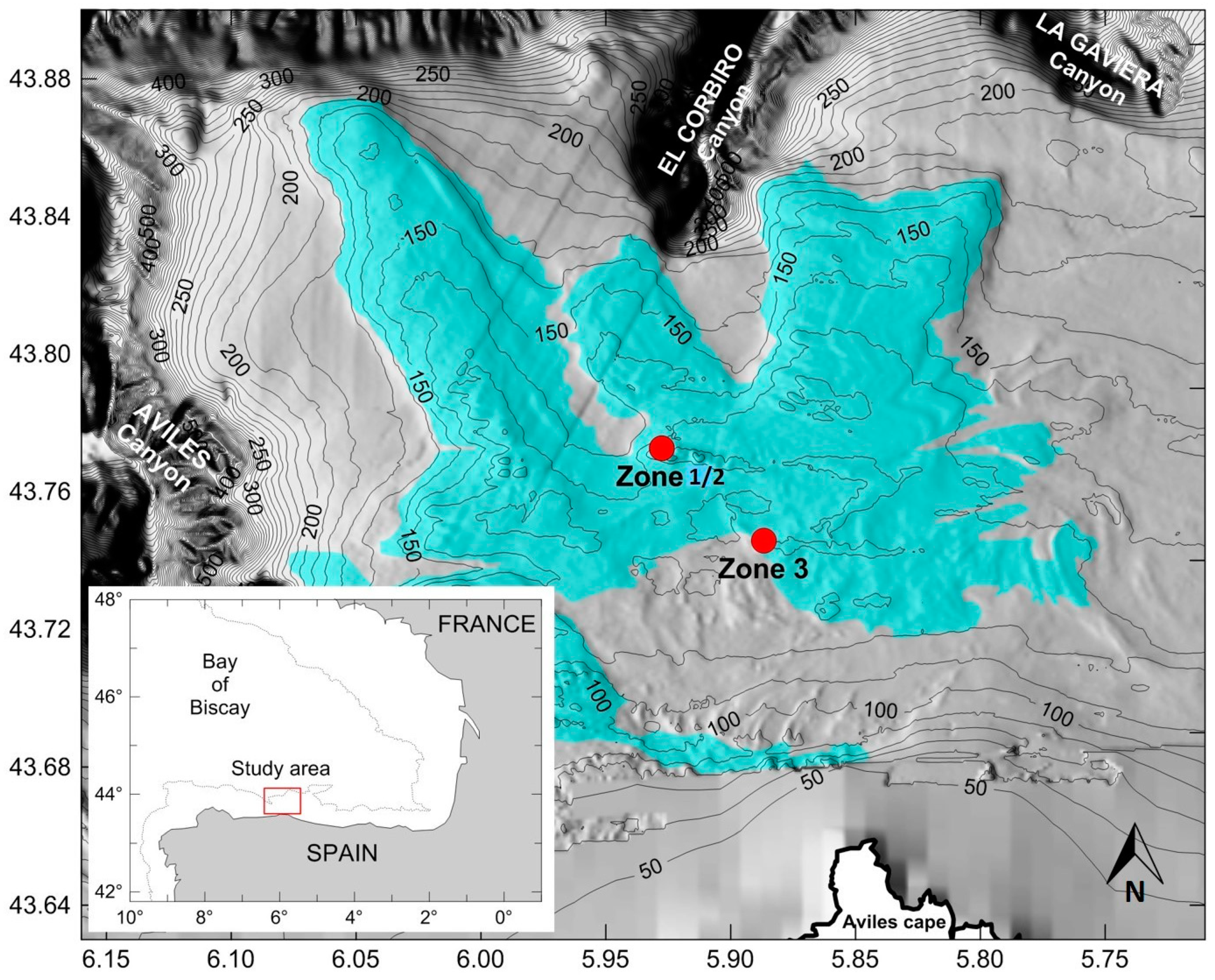
The area of the Bay of Biscay continental shelf located in the headwaters of the Avilés Canyon System (ACS) is characterized by rocky outcrops (Figure 1). This is mainly due to the sedimentary transport mechanisms associated with the ACS’s oceanographic dynamics. Throughout the entire Bay of Biscay, the continental shelf is generally narrow; a typical characteristic feature of compressive continental margins [50]. Its width varies from 12 km, at the head of the Avilés Canyon (AC), to 40 km, with maximum depths of about 200 m and exceptionally as high as 300 m east of the AC. The slope varies gently, ranging from 0 to less than 1º. The area is highly affected by tectonic action, with interference of various strain directions [51]. This strong tectonic influence results in a very irregular continental shelf edge, with incoming and outgoing directions oblique to the coastline. In general, the existence of strong currents in the Bay of Biscay continental shelf prevents the accumulation of large sedimentary deposits on this rocky area. The materials are dragged and channeled through the canyons, resulting in a platform with low sedimentary thickness.

This area is currently declared a site of community importance (SCI) in the context of the Natura 2000 network, mainly due to the existence of coral reefs [52].

2.2. Survey Description and Image Acquisition

Images were obtained from 3 test zones (Figure 1) in two different trips, each associated with the following projects; Zone 1 and Zone 2: ECOMARG 2017, monitoring of the marine protected area of El Cachucho and Zone 3: LIFE IP INTEMARES, Action A4, Diagnosis of the impact of human activities and climate change on marine RN 2000 and proposals to control, eliminate or mitigate its effects.

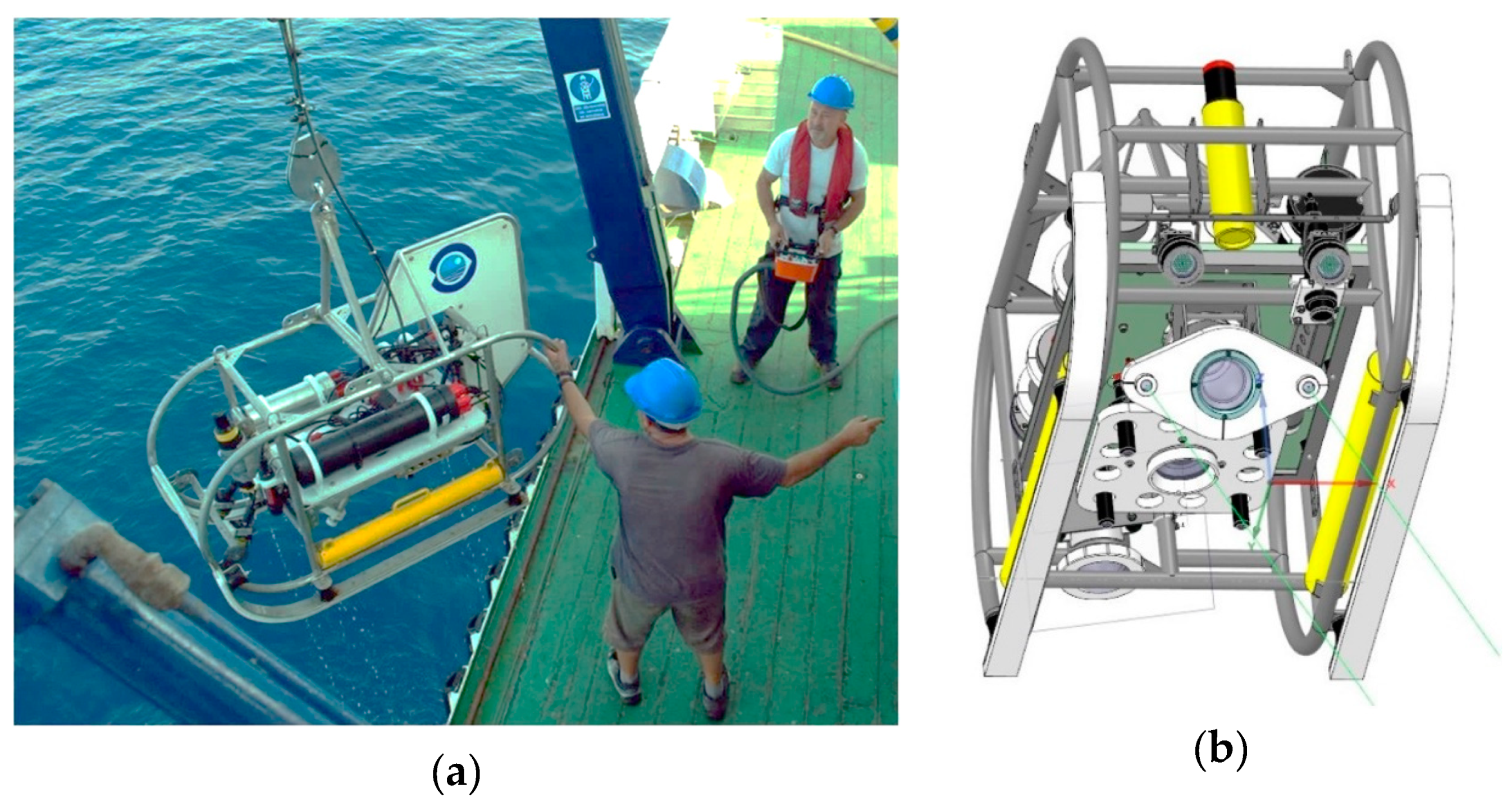
The images analyzed in this study were obtained using the remotely operated towed vehicle (ROTV) Politolana (Figure 2). The ROTV Politolana, designed by the Santander Oceanographic Center of the Spanish Institute of Oceanography (IEO), is a robust submarine towed vehicle designed to study the deep-sea floor using photogrammetric methods [53]. The vehicle can be operated down to a maximum of 2000-m depth. In this case, transects were carried out navigating at a 0.8–1.0 knots at 2–4 m over the sea floor. The vehicle has bidirectional telemetry to control the submerged instruments (altimeter, CTD probe, compass, video and still camera control) and sends data to the surface control unit in real time. This vehicle acquires both still pictures and HD videos simultaneously, synchronizing them with measurements of the existing environmental conditions.

Absolute positioning of the vehicle is provided by a Kongsberg HiPAP 502 super-(ultra)-short base line (SSBL). This fully omni directional system can be pointed in any direction below the vessel, as the transducer has the shape of a sphere and an operating area of 200°. The ROTV is positioned by an acoustically operated transponder. Ad hoc designed software performs synchronization of data in real time. ocean floor observation protocol—OFOP software [54] processes the observation files subsequently and merges them with additional sensor data, which are corrected for space and time offsets and finally splined producing a complete data set for each individual deployment.

Video transects of Zone 1 and Zone 2, were recorded in July 2017 during the ECOMARG-2017 survey (E0717_TV02); at a range of depths around 125 m. The video-camera used was a Full HD video camera (Sony HD-700-CX), at 45° with respect to the seabed and two LED lights (12,600 lumens/6000° Kelvin) were attached to the image system. The system was equipped with 2 parallel laser beams separated by a constant distance of 20 cm (Figure 2b). This distance provides a method to scale and validate the geometric uncertainty of the resulting model. The two sections of video transect analyzed in this study were about 100 m and 50 m long for Zone 1 and Zone 2, respectively. The footprint on the seabed was around 3 m wide; this imaging swath varies depending on the height of flight over the seabed and its topography.

High resolution photographs used for Zone 3 were acquired during the INTEMARES A4 Avilés 2018 survey (IA418_TF27); in a range of depths about 120 m. The ROTV Politolana is fitted with a Sony Alfa 7 camera (24 megapixels) with two LED lights, at zenithal position. The system was equipped with 4 parallel laser beams separated by a constant distance of 25 cm that provides a method to scale the images (Figure 2b). The equipment takes pictures with a time-lapse of 0.5 s obtaining representative data of the habitat and benthic communities to be characterized and a collection of highly overlapping images that register a complete image of the sea floor.

2.3. 3D Image Reconstruction and Digital Surface Model

Video sections were decomposed into thousands of geopositioned overlapping images. These video frames and photographs were processed using photogrammetric Pix4D MapperPro software (Pix4D SA, Switzerland). This software carries out advanced automatic triangulation based purely on image content and an optimization technique [55]. The triangulation algorithm is based on binary local key points, searching for matching points by analyzing all images. Those matching points, as well as approximate values of image position and orientation provided by the Politolana telemetry system, are used in a bundle adjustment to reconstruct the exact position and orientation of the camera for every acquired image. For this study, the focal length, principal point and radial/tangential distortions of the cameras were set as initial theoretical values, while the final internal and exterior orientation parameters were determined by bundle adjustment processing.

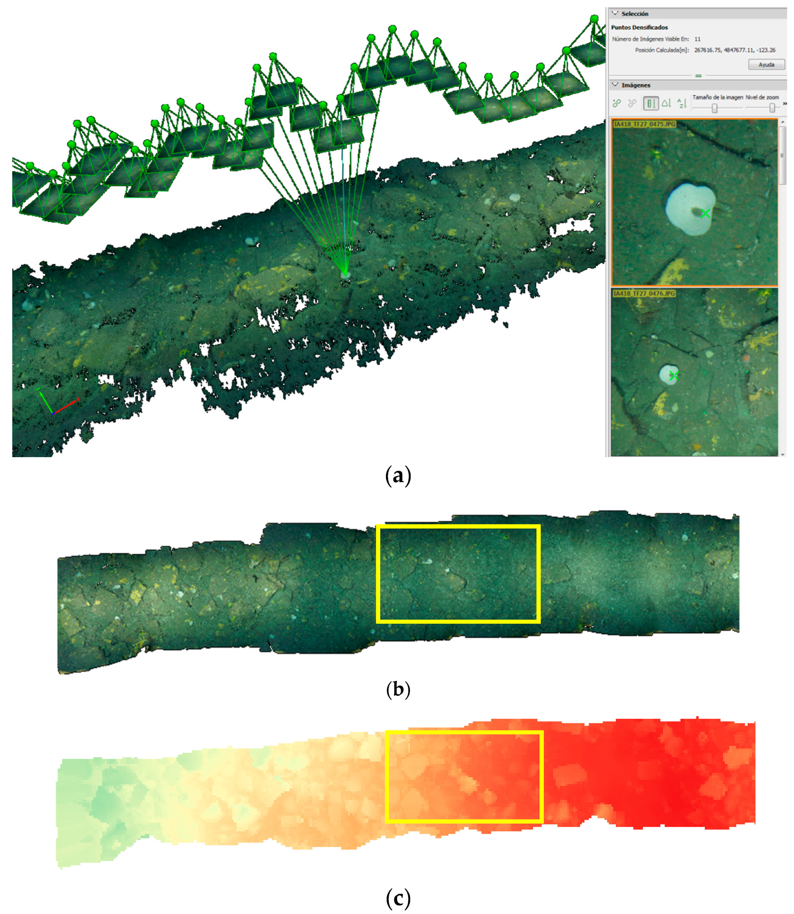
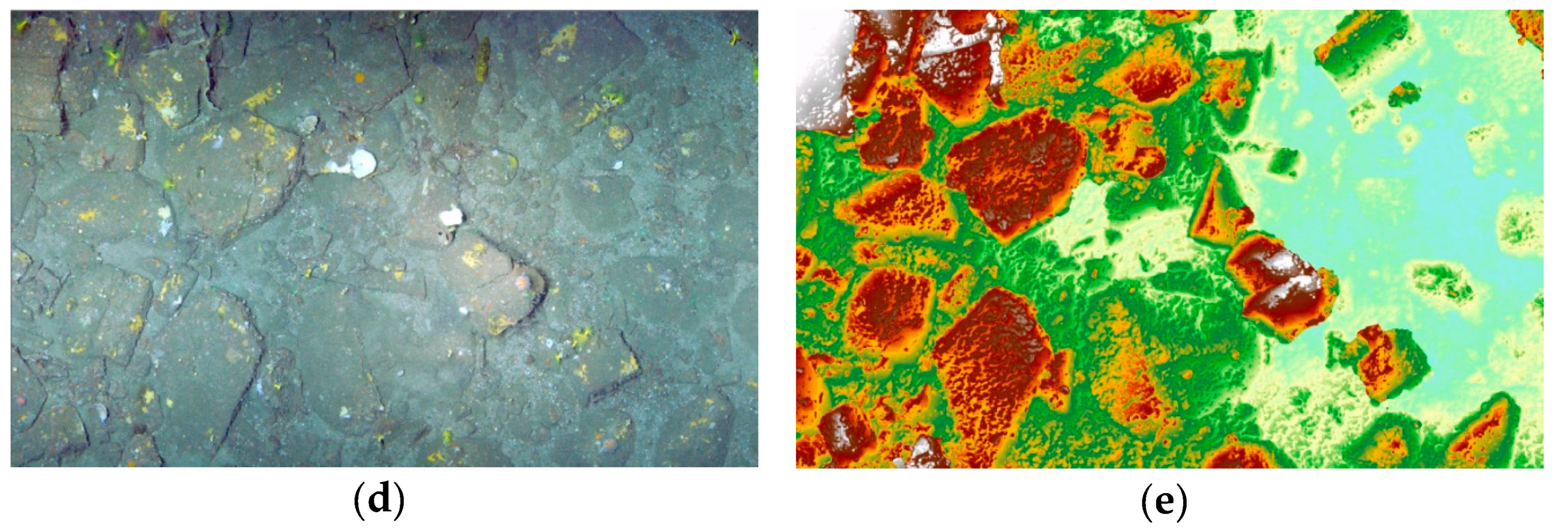
The distance between parallel laser beams (20 cm apart in video frames and 25 cm apart in photographs) is used as reference scale. Several scale constraints are used to fine rescale and optimize the project. With this complete automated integration of tie point measurements, camera calibration, position data given by the cameras and scale constraints, the software provides 3D dense point clouds (Figure 3a), orthomosaics (Figure 3b,d) and digital surface models (DSM) (Figure 3c,e). The products derived from the sea floor morphology, such as maps of slope, aspect, rugosity, curvature, etc. can be extracted from the DSM in a simple way. Since all the information is geo-referenced in a cartographic system (UTM-WGS84), all geographic layers obtained can be included in a GIS environment.

The 3D point cloud is a cartographic product that contains coordinates (XYZ) of the points and color information, enabling subsequent morphometric analysis. The point cloud processing is used to extract DSM. The maximum spatial resolution ground sampling distance (GSD) was used to produce orthomosaics. These very-high resolution orthomosaics are used to annotate species presence location. To generate a DSM model, the resolution was resampled to avoid the size of the individual specimens contributing to differences in DSM.

2.4. Terrain Analysis

Spatial terrain properties describe the complexity of the habitat and condition the location of the specimens on the seabed. To quantify these spatial properties, DSMs of the surveyed sites were exported from Pix4D software into R.

Then, this bathymetric layer was used to calculate the terrain descriptors in R software; aspect, slope, roughness, curvature and bathymetric position index (BPI) of the terrain model (Figure 4). Aspect indicates the direction that slopes are facing, the direction of the surface expressed in two components (north and east). Slope is the vertical gradient of a surface, expressed in degrees. Terrain–surface roughness is a morphometric measure expressing how heterogeneous a surface is. Roughness is the difference between the minimum and maximum bathymetry values for a given surface area. Curvature in marine environment expresses the acceleration, deceleration, convergence and divergence of flow across a surface and therefore indicates areas influenced by erosion or deposition processes. Finally, BPI is the difference in bathymetry between a central cell and the mean value of a given group of surrounding cells.

These morphometric terrain descriptors were generated from a resampled low resolution DSM. This operation means that presence of the specimens does not contribute to generating differences in the results.

2.5. Faunal Presences

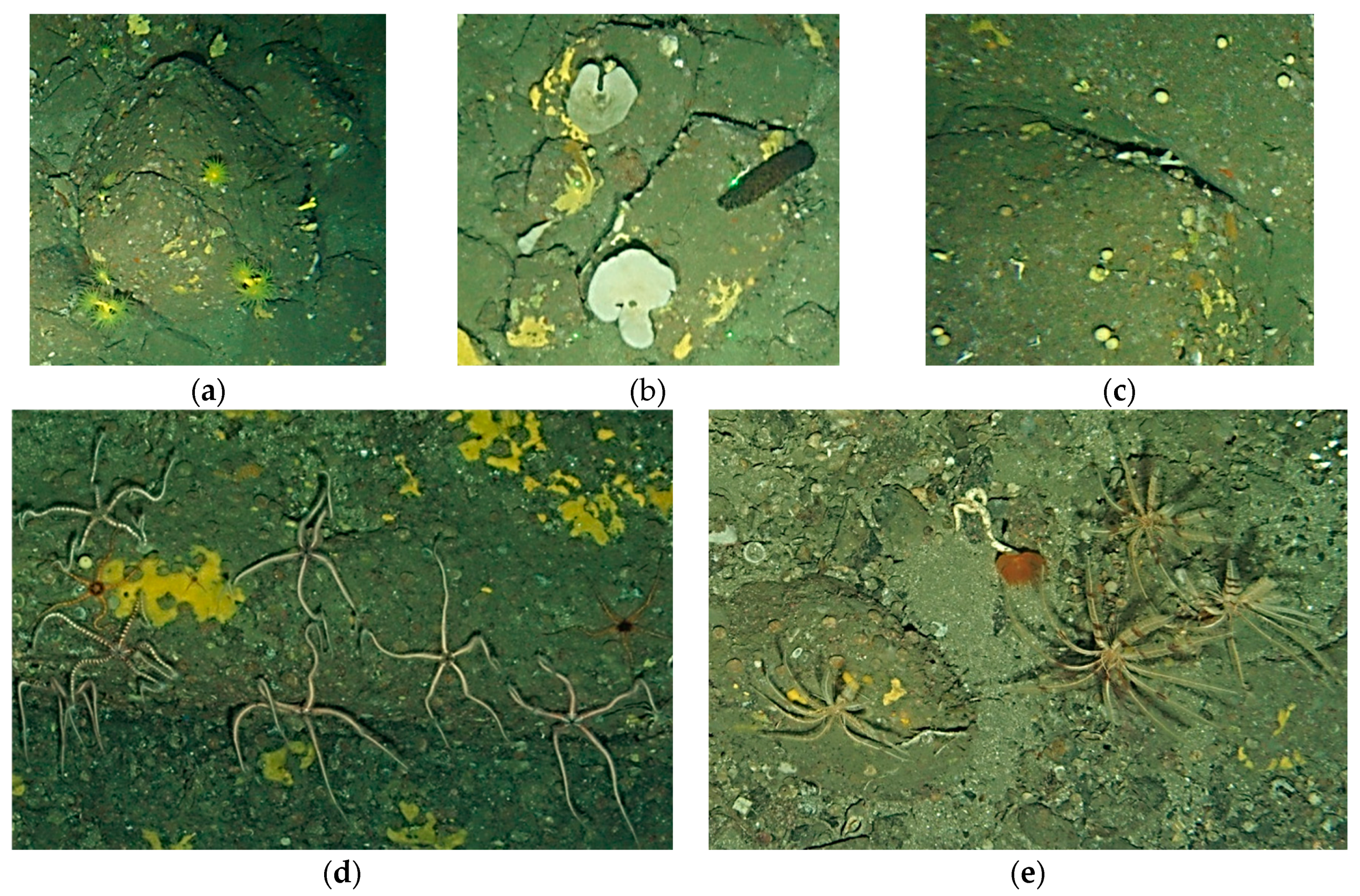
The target species for this study were those that, due to their size or morphologic characteristics, are easily identified in the images. Specifically: one cnidarian (Dendrophyllia cornigera (Lamarck 1816)), two sponge morphotypes (Artemisina transiens (Topsent, 1890) and Phakellia ventilabrum (Linnaeus, 1767)), three brittle stars (Ophiothrix fragilis (Abildgaard in O.F. Müller, 1789), Ophiothrix sp. III (sensu Taboada & Perez-Portela, 2016) and Ophiura ophiura (Linnaeus, 1758) and one feather star (Leptometra celtica (M’Andrew & Barrett, 1857)).

The yellow scleractinian coral D. cornigera (Figure 5a), is well known from Ireland to the Cape Verde Islands, including in the Azores archipelago and the Mediterranean Sea, with a bathymetric distribution ranging from 80 to 600 m. It is widely distributed in the whole Bay of Biscay and nearby areas.

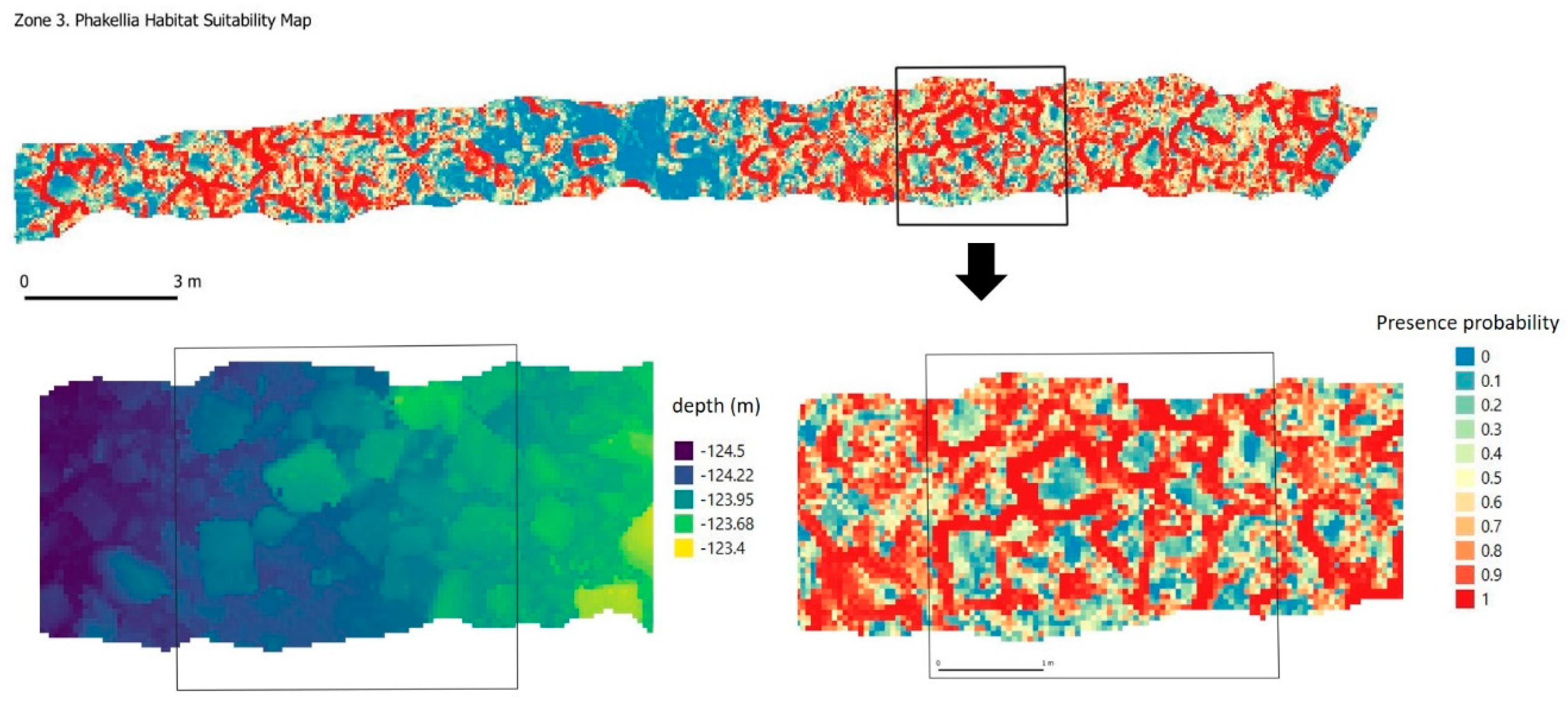
P. ventilabrum (Figure 5b) is a species that is characteristic of the sponge communities on deep circalittoral rock (EUNIS habitat code A4.12), among others. It is a Demospongiae sponge with a funnel shape or flabelliform, whitish color and a wide distribution in the North Atlantic Ocean, Arctic and Mediterranean Sea; it is found at depths of 10–1863 m.

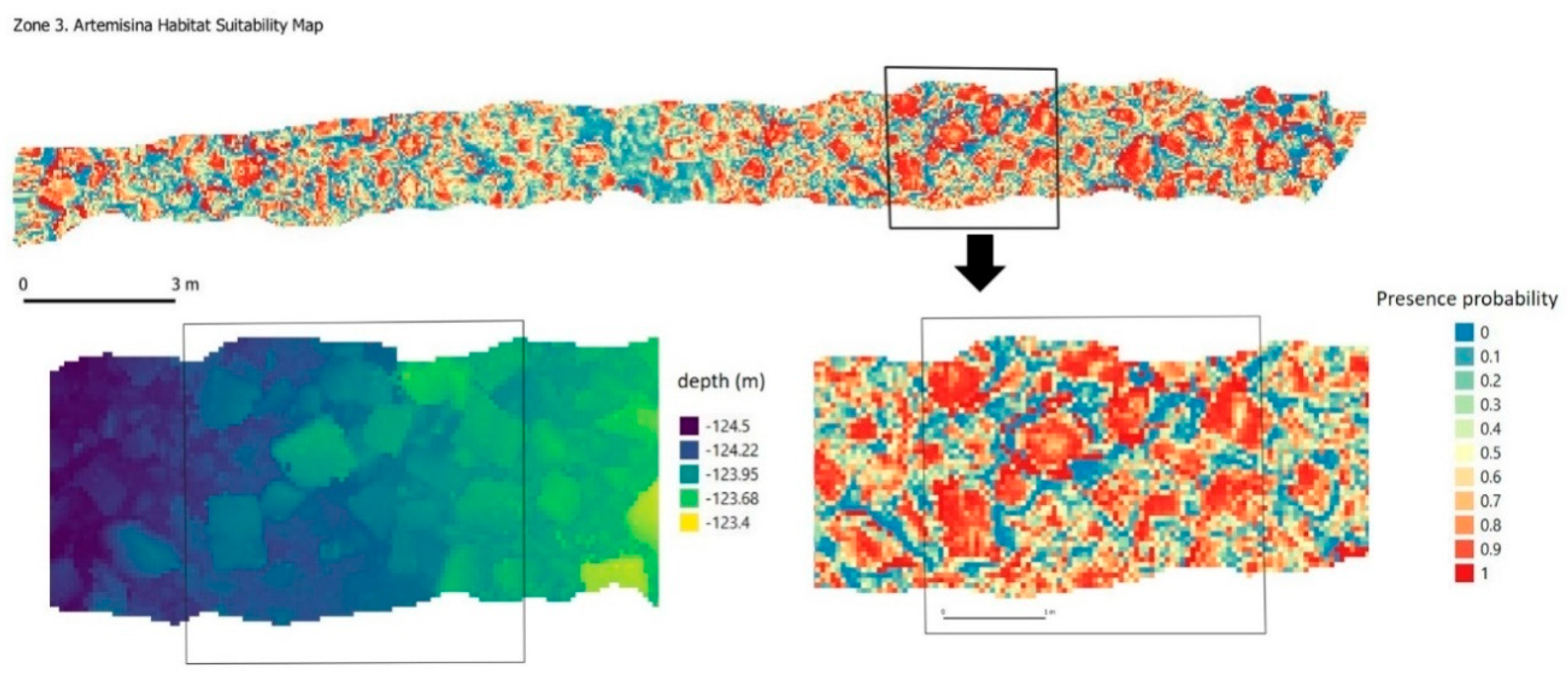
A. transiens (Figure 5c) is a globular pedunculated sponge with several slightly raised apical oscules with a main body with a spherical to elliptical shape. It is found from 35 to 126 m in depth and the density of these sponge grounds can reach up to 50—60 ind/m², with the appearance of ‘mushroom fields’ (Ríos et al. 2018).

O. fragilis (Figure 5d) is a species characteristic of echinoderms and crustose communities on circalittoral rock (EUNIS habitat code A4.21). With a wide range of colors, the specimens from ACS are green, brown and/or orange alive. The color of specimens of Ophiothrix sp. III (Figure 5d) (Taboada & Perez-Portela, 2016) from ACS is principally orange alive, but the disc is pale pink and white. O. ophiura (Figure 5d) is a species characteristic of the fine circalittoral sand Habitat (EUNIS habitat code A5.25). The color of specimens from ACS is pink. This species lives from intertidal down to more than 200 m, on sand or muddy sand. In ACS, it lives up to a maximum depth of 240 m, in patches of fine sand.

L. celtica (Figure 5e) is an unstacked crinoid distributed in northeast waters of the Atlantic Ocean, West and South Africa and Mediterranean Sea. The ability of these echinoderms to adapt to different types of habitats and depths makes this species extraordinarily abundant in the Bay of Biscay Canyons, where it can colonize rocky bottoms from the circalittoral floor, at 80 m, down to more than 1000 m in submarine canyons and even over coral reefs in regressive state [52].

These species are annotated in the three zones on a portion of high-resolution orthomosaics generated from 3D reconstruction. In addition, for the 3 zones and for all the selected species, absences were generated manually to improve the estimation of the predictive statistical models.

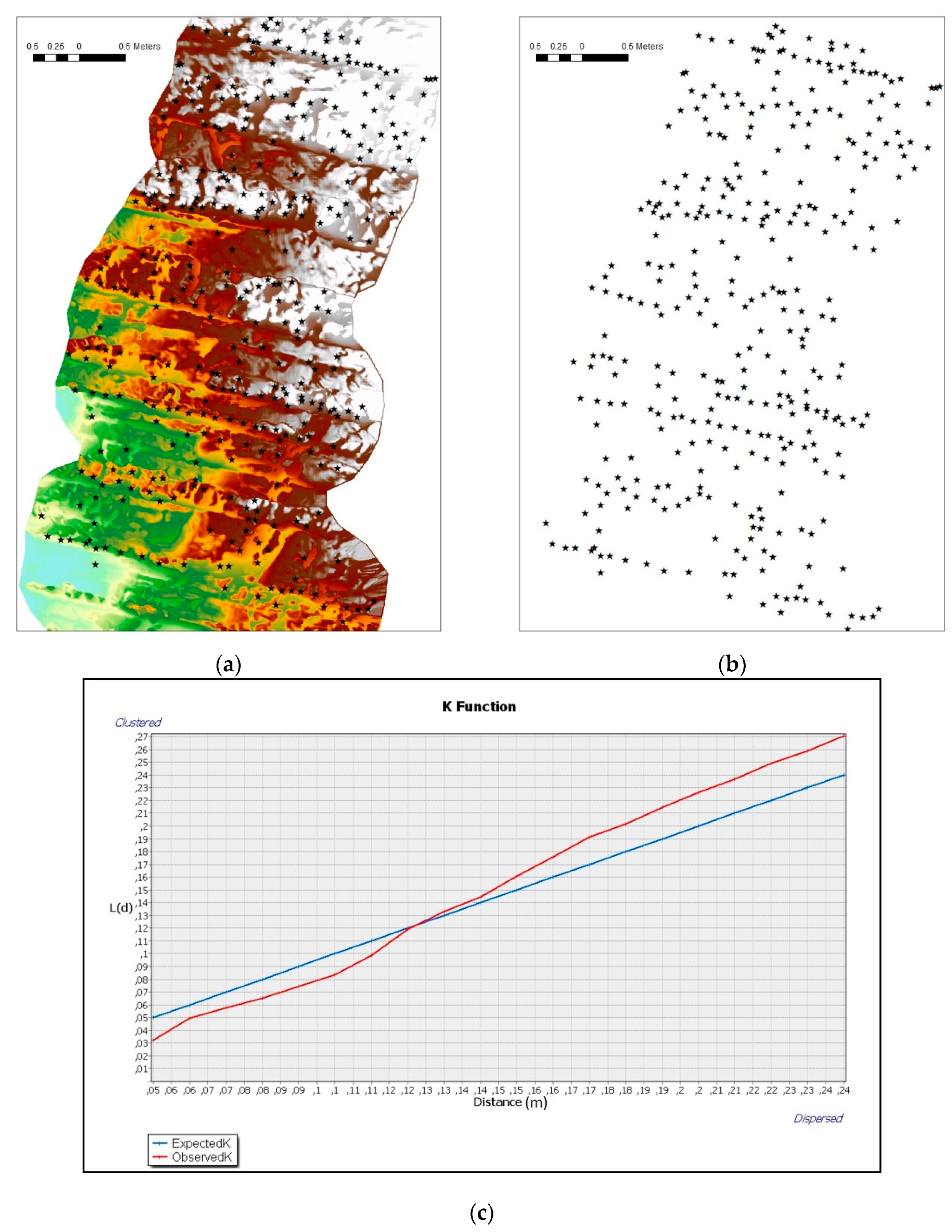
To analyze the spatial pattern distributions of these species within the areas, multi-distance spatial cluster analysis is used. This approach is based on Ripley’s K function [56]. A distinguishing feature of this method is that it summarizes spatial dependence (feature clustering or feature dispersion) over a range of distances. Therefore, the selection of an appropriate scale of analysis is necessary. This analysis enables the determination of whether the phenomenon of interest (e.g., positions of specimens) appears to be dispersed, clustered or randomly distributed throughout the study area using very high-resolution information (~cm).

2.6. Significant Terrain Variables and Habitat Suitability Model

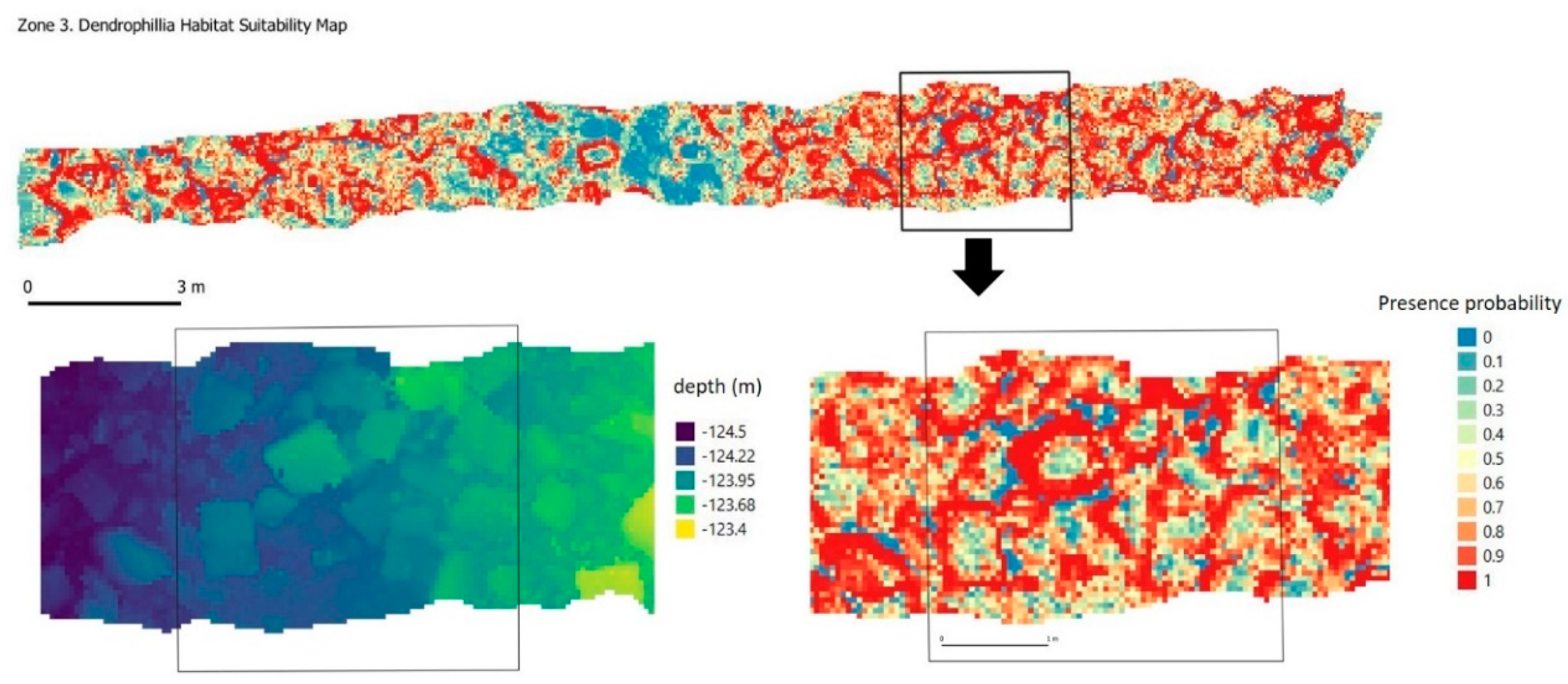
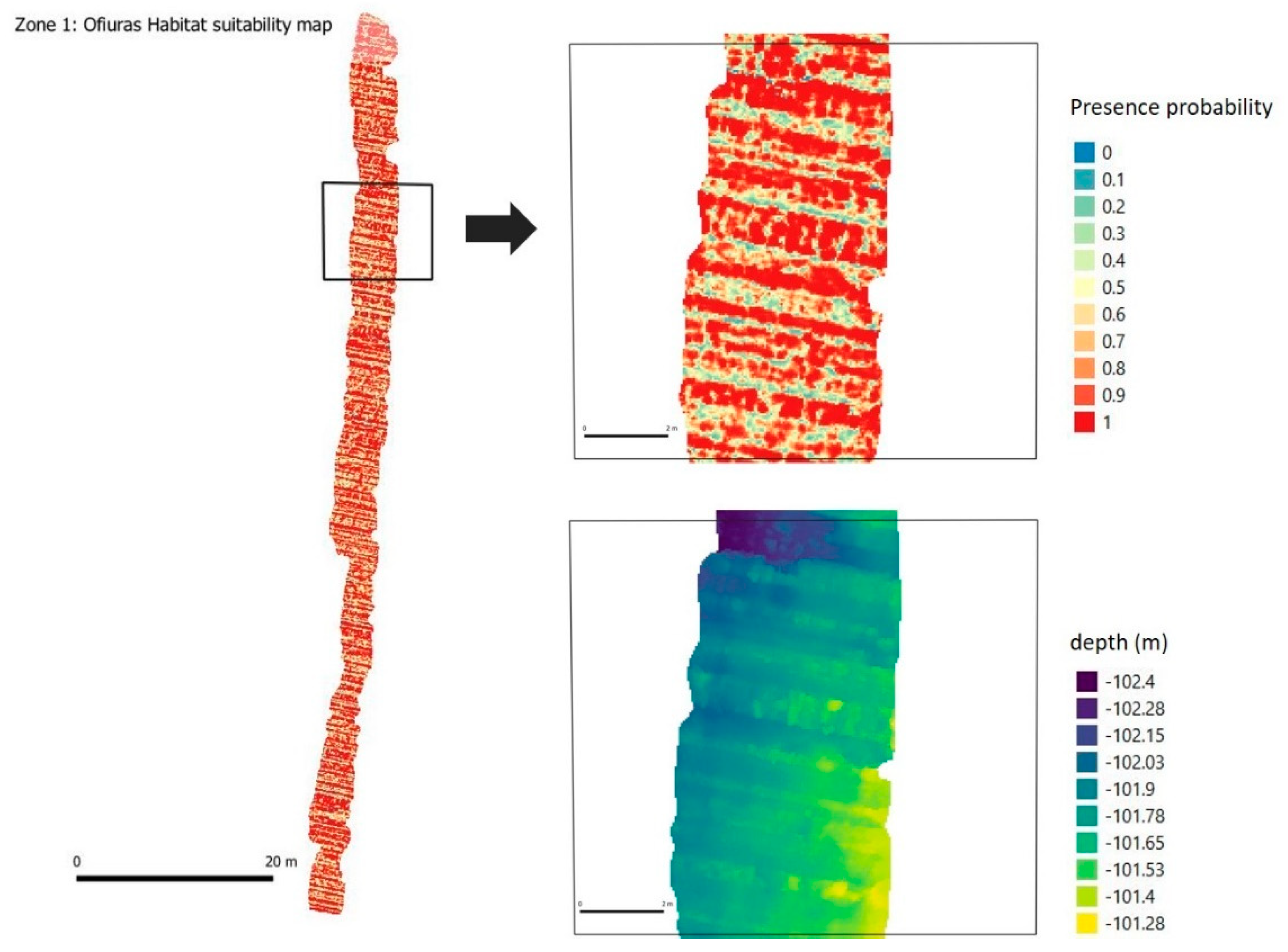
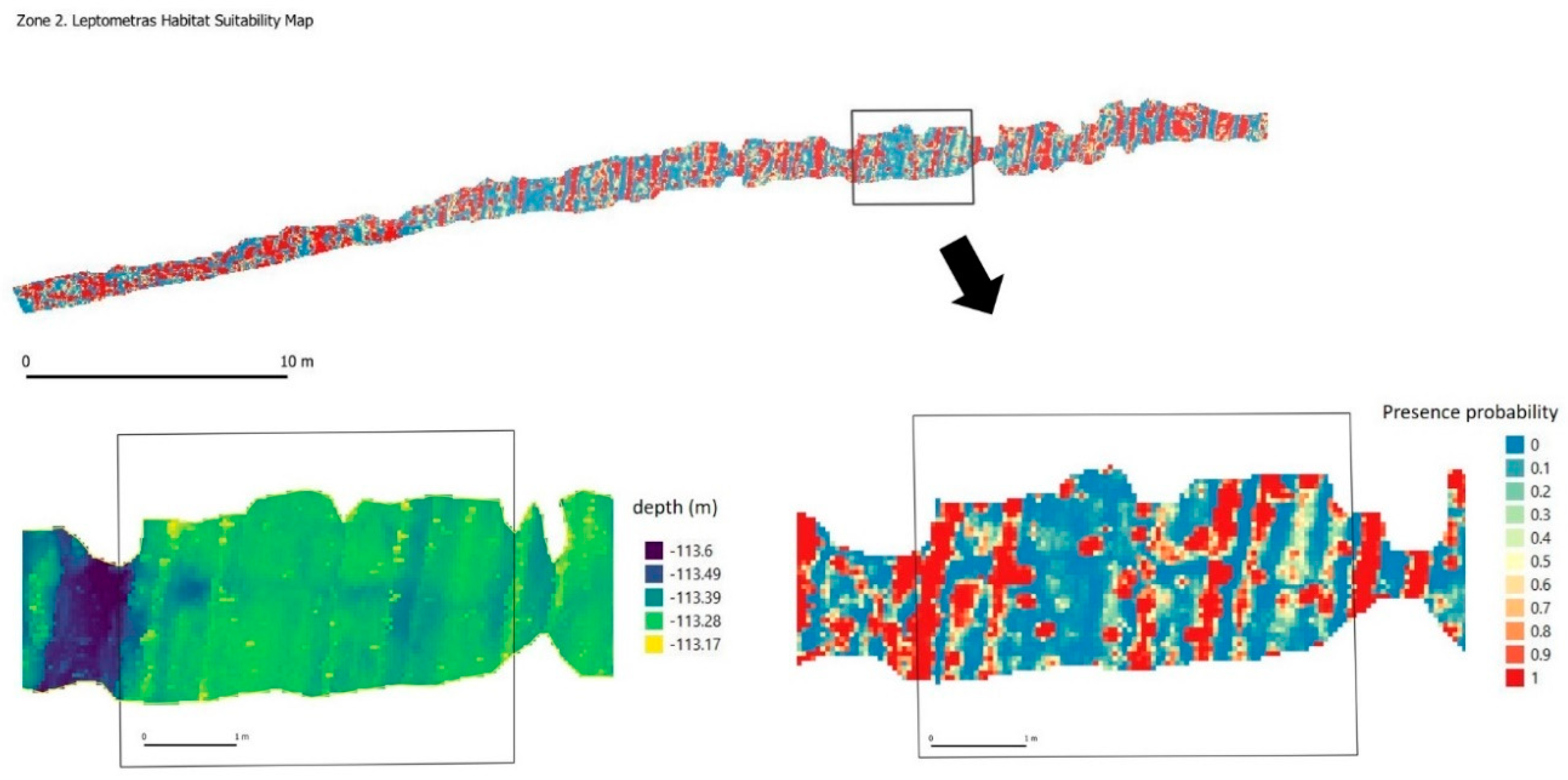
The habitat suitability model technique was applied to create maps for each target species, showing spatial distributions according to probability values. Generalized additive models (GAMs) are widely used statistical models of species distribution in habitat and environmental management modeling as they enable the incorporation of nonlinearity.

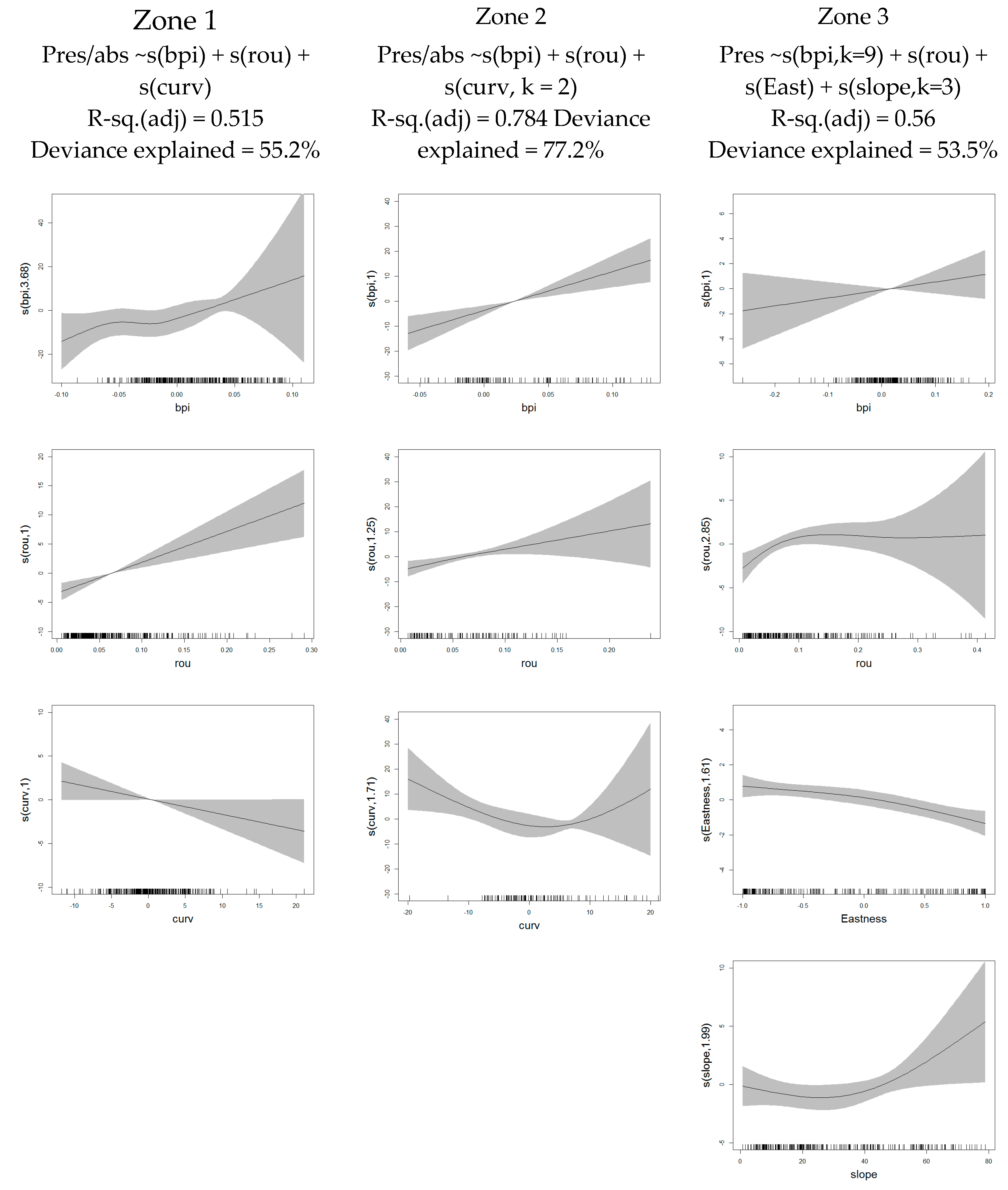
GAMs were used to determine which high-resolution-derived terrain variables were most useful in explaining observed spatial patterns and habitat distribution of the selected species. The environmental variables used were extracted from high-resolution 3D point clouds. First, to detect multicolinearity among the different predictors, a variance inflation factor (VIF) was established and the correlated variables discarded so inflation due to colinearity could be avoided. Second, univariate GAMs were applied to select the variables that have great influence on the presence of specimens. Third, the variance and the level of significance (p-value < 0.05) were used to select the variables that have influence on the final predictive model. Finally, once the significant variables were selected, we could combine these environmental variables derived exclusively from the terrain descriptors to obtain the most significant predictors that will help to explain the location of the species at the centimetric level.

After the models were defined, a similar GAM approach was used to predict relative abundance of selected species throughout three test zones, based on the defined models, estimation of presence and absence located in a portion of orthomosaic and the micro-bathymetric conditions.

Validation of predictive models was achieved using AUC (area under curve) tests for the presence/absence that assess misclassification rate. AUC measures the ability of model predictions to discriminate between observed presence and absence for a test dataset. It is independent of the threshold and takes into account the sensitivity (true positives), as well as specificity (false negatives).

2.7. First Approximation of Automatic Image Annotation of Species Using Deep-Learning

A deep learning-based algorithm was tested for the automatic annotation of specimens in the very high-resolution orthomosaic created for Zone 3. As both species identification and location is needed, an “object detection” variant of a convolutional neural network (CNN) was chosen. YOLO v4 (You Only Look Once, version 4) architecture [57] was used. It is based on a CSPDarknet53 backbone image prediction CNN network and a YOLO v3 head to predict the size and location of the object’s bounding boxes. This particular approach embraces several recent improvements in the architecture and training pipeline of deep-learning algorithms that result in very good precision and fast inference times.

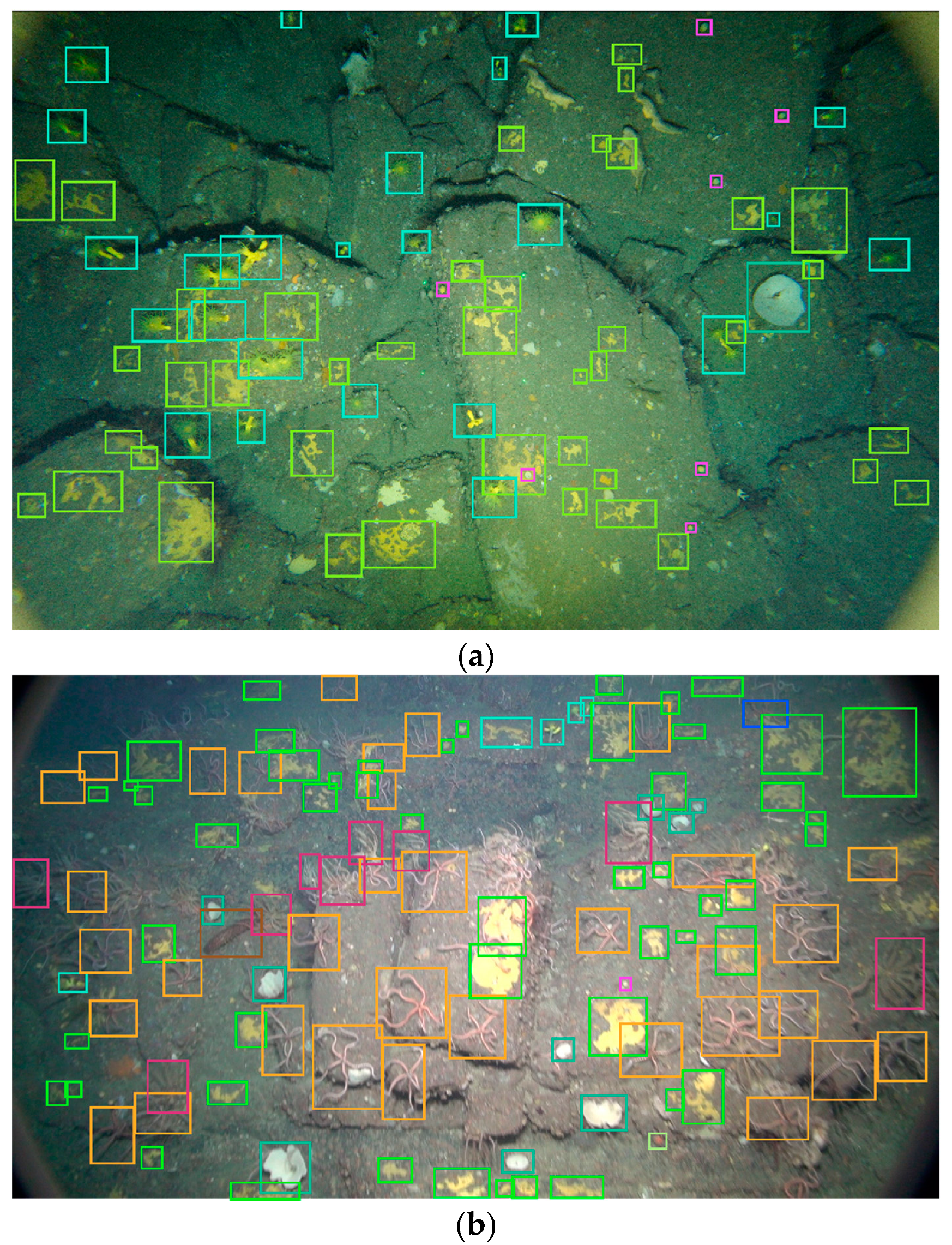
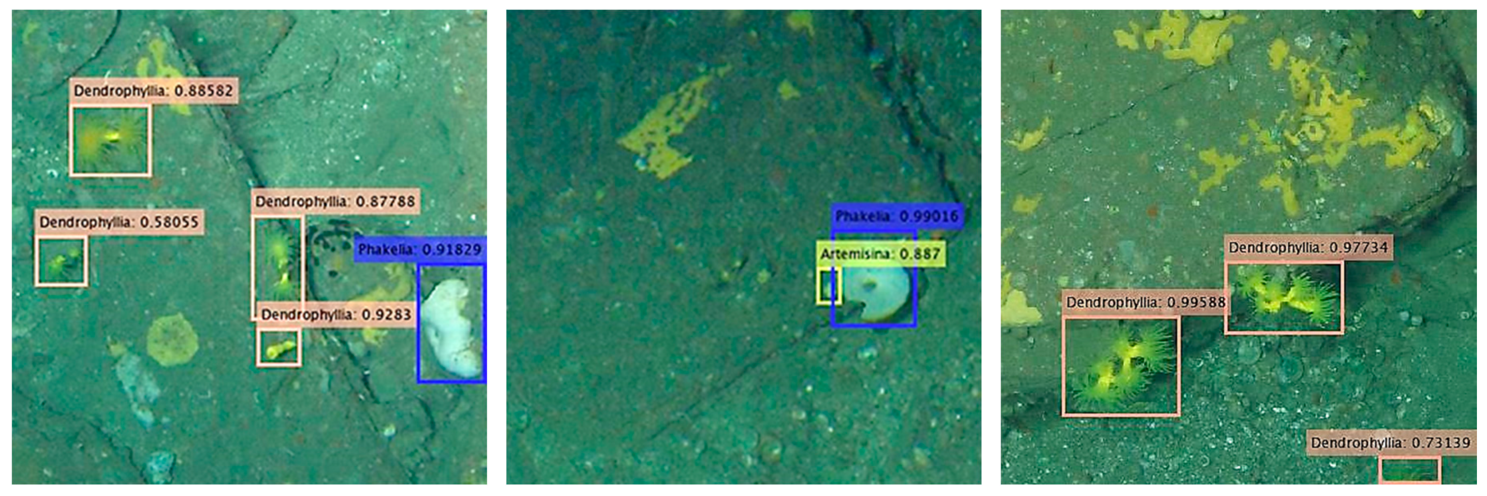
For the training, a network previously trained on the MS COCO dataset (80 classes of common objects) was chosen as the starting point. The supervised procedure uses a dataset of 65 high-resolution images (both full HD video frames and 24Mpx photographs) from several circalittoral rocky floors. The images were manually annotated by an expert using the web service Supervisely (http://supervise.ly). The manual annotation (Figure 6) was performed on seven species;, but for the training, only the three structural species in Zone 3 (A. transiens, D. cornigera and P. ventilabrum) were considered, resulting in 532 specimens, 705 colonies and 250 specimens of each species, respectively. From the high resolution images, a custom script generates the training and validation datasets (80%/20%) of 416x416px cropped images, adding the following data augmentation transformations: random shift, horizontal flip, vertical flip, resizing, brightness and color variations. Both the selection of annotated object and the amount of data augmentation is adjusted dynamically by the script to reduce the resulting class imbalance, which is a problem for this kind of datasets due to the huge difference in the number of specimens of the different species. The training procedure was performed with the default hyperparameters suggested by the yolov4 author [57], although some of them were fine-tuned looking for the best performance. The final values of the most important ones are: Learning rate = 0.001, Batch size = 16, Subdivisions = 8, native size = 416 × 416px.

The results of orthomosaic annotation processing obtained using this automatic process was validated against the manual annotation by an expert generated as input data for predictive habitat modeling.

3. Results

3.1. 3D Model, Digital Surface Model and Terrain Variables

Individual 3D models were reconstructed for three study zones. Trajectory reconstruction and automatic tie point extractions were performed and a re-optimization of the model based on scales obtained from parallel laser beams was carried out. From these measurements, dense point clouds can be processed afterwards in high-density mode. A basic description of the characteristics of the 3D point clouds and orthomosaic processing performed is shown in

Table 1. Basic data regarding the image dataset and the 3D point cloud densification process.

Summary	Zone 1	Zone 2	Zone 3
Longitude of video section (m)	91	48	25
Area covered (m2)	421.5	93.3	60.1
Average Ground Sampling Distance - GSD (cm)	0.23	0.14	0.05
Number of calibrated images	341	191	101
Median of matches per calibrated image	4268	4207	7290
Number of 3D densified Points	21833998	11590084	19864272
Average density points (per m3)	709,403	2.44 × 106	1.76 × 107

.

Several scales were used for re-optimization of the geometric fitting of the models showing very low uncertainty (

Table 2. Summary of scales of geometric uncertainty in 3D models.

Summary	Zone 1	Zone 2	Zone 3
Mean reprojection error (pixels)	0.209	0.202	0.196
Number of scales	9	2	3
Initial length (m)	0.200	0.200	0.250
Mean computed length error (m)	0.005	0.017	0.018
Mean relative camera position uncertainties (m):
X	0.023	0.006	0.002
Y	0.034	0.008	0.004
Z	0.029	0.007	0.002

).

According to Table 1, the average of GSDs in different zones is always below 0.5 cm; so, although the presence of specimens is annotated in a maximum-resolution orthomosaic; in areas with faunal aggregations or specimens with considerable size, the extracted terrain descriptors are derived from the surface of these aggregations or these species. Based on the resolution of our model and the sizes of selected species specimens, all terrain descriptors were resampled to a pixel size of 5 cm to test for small-scale terrain morphometric characteristics. Therefore, from the digital surface model, slope, aspect (north and east), BPI, curvature and rugosity were obtained.

3.2. Environmental Characteristics of Studied Sites and Faunal Presence

The study areas are composed of a mainly rocky bottom, with some small sediment patches with very low slopes, which are always less than 3%. In both Zone 1 and Zone 2, there are small steps of approximately 20 cm, which are arranged in a transverse direction to the transect and are regularly spaced along the transect (Figure 7a,b). This seafloor morphology is common in this zone. In Zone 3 the bottom consists of adjacent rocky blocks of various sizes, between 10 and 20 cm in height (Figure 7c). Some small sedimentary-bottomed patches appear from time-to-time, without the presence of these blocks of rock that, given their sandy composition, do not present highlights or abrupt changes in elevation.

The target species in this study were annotated on portions of high-resolution orthomosaics in all study areas using QGis. In this way, a list of coordinates identifies the locations of presence/absence of specimens. An area of 20 m² was selected in Zone 1; 341 specimens of the dominant species of brittle stars was annotated, obtaining a density of 17 specimens per m². An area of 12 m² was selected in Zone 2; 93 specimens of the L. celtica were annotated, obtaining a density of 7.75 specimens per m².

Finally, in Zone 3 there is no unique predominant species, but there is a concentration of different species, among which three (D. cornigera, P. ventilabrum and A. trasiens) were selected. In the high-resolution orthomosaic covering an area of 60 m², the presence of all the specimens of these species was annotated: 206 colonies of D. cornigera (3.43 colonies/m²), 56 specimens of P. ventilabrum (0.93 specimens/m²) and 120 specimens of A. transiens (2 specimens/m²). These coordinate lists of the instances was used as the input layer for the habitat suitability models.

Ripley’s K indicated the distribution of ophiuroids is more clustered than a random distribution at distances greater than 0.13 m in Zone 1 (Figure 8), so the presence of ophiuroids displays distribution clustering points; while at smaller distances, the points were more dispersed than a random distribution. In Zone 2 the analysis of clustering of L. celtica positions shows a dispersed distribution over the sea floor at any distance from 0.05 to 1.5 metros (Figure 8b). In Zone 3 both the selected species, A. transiens and D. cornigera display a more clustered than random distribution at distances less than 1.3 m and P. ventilabrum shows this clustered distribution at distances from 0.2 m to 1.3 m.

3.3. Significant Terrain Variables and Habitat Suitability Model

The depth variable was eliminated since at these fine scales the absolute altimetry differences within the same area are negligible as a condition that a species is present or not at a specific point. Therefore, the initial set of 6 environmental predictors: slope, aspect (north and east), BPI, rugosity and curvature were reduced to select the most explicative variables using a univariate approach. The variance inflation factors (VIF) showed collinearity between roughness and slope for Zones 1 and 2, so we avoided using slope as it had the highest VIF. Collinearity was not detected between terrain variables in Zone 3.

Deviance explained and adjusted R squared of univariate GAM models are shown on

Table 3. Results of univariable adjustment for terrain variables for Zone 1 and Zone 2. Shaded in gray, the predictors used for the final model of each species.

R-sq.(adj)/Deviance Explained (%)
Terrain Variables	Zone 1	Zone 2
Aspect (North)	0.014/2.54	0.01/0.22
Aspect (East)	0.015/2.8	0.02/4.36
Bathymetric position index (BPI)	0.320/38.7	0.45/43.7
Curvature	0.099/14.6	0.33/31.5
Rugosity	0.205/25.2	0.57/50.2
Final model	0.515/55.2	0.784/77.2
AUC	0.951	0.986

for the most representative species of Zone 1 and Zone 2, with a unique selected species for each zone. The most important predictors for these areas are the bathymetric position index and the roughness. The first one explains about 40% of the variance of both zones. As for roughness, its contribution to the final model of Zone 2 is highly relevant, with more than 50% of the variance explained in the univariate GAM and it is also relevant for Zone 1, explaining 25% of the variance.

The univariate GAM results for Zone 3 are presented by target species in

Table 4. Results of univariate and final model general additive model (GAM) adjustment and deviance explained for terrain variables for Zone 3. Shaded in gray, the predictors used for the final model of each species.

R-sq.(adj)/Deviance Explained (%)
Terrain Variables	D. cornigera	A. transiens	P. ventilabrum
Northness	Not significant	0.03/3.51	0.07/5.66
Eastness	0.1/8.14	0.03/2.6	0.28/22.8
BPI	0.11/11.1	0.2/16.4	0.26/22.6
Curvature	0.08/8.77	0.07/6.31	0.29/25.9
Rugosity	0.34/30.5	0.1/9.21	0.61/53.6
Slope	0.22/22.5	0.04/4.25	0.49/43.7
Final model	0.56/53.5	0.45/40.9	0.66/62.4
AUC	0.941	0.894	0.959

. The most important predictor in this area for D. cornigera is the roughness, explaining about 30% of the variance, followed by the slope, which explains about 22%. As for P. ventilabrum univariate models, roughness is the most important predictor with a value of 53.6% of the variance explained, followed by slope, which displays about 43%. In the case of A. transiens, the univariate GAM shows 16% and 9% of explained variance for bathymetric position index and for roughness, respectively. Although these values are lower than the previous ones, they are the most important for this species.

As for the final models of the three zones (Figure 9), three predictors explain 55.2% of the variance in Zone 1, roughness, BPI and curvature. The same variables explain 77.2% of the variance in Zone 2 and finally, in the case of Zone 3, 53.3% of the variance is explained by roughness, BPI, Eastness and slope. AUC values (Table 3 and Table 4) very close to 0.9 in all cases show very high reliability of predictions.

The probability of occurrence of the species studied in all the areas increases directly as the BPI and roughness become higher. However, to a certain extent, when presence decreases, confidence bands become wider. Thus, the presence of the brittle stars is not relevant above a BPI value of 0.05 in Zone 1, 0.1 in Zones 2 and 3 or above a roughness value of 0.1. On the other hand, the curvature has a negative relationship with occurrence in Zones 1 and 2; and Eastness and slope and the rest of the significant predictors of Zone 3, do not display a clear tendency.

The models designed enabled the generation of detailed maps with the spatial distributions expressed as probability values (Figure 10, Figure 11, Figure 12, Figure 13 and Figure 14), identifying the environmental characteristics required for each of the selected species. These models were run with data based on the presence and absence of the selected species annotated in very high spatial resolution orthomosaic and with representative values of abundance in the area.

In general terms we can summarize by indicating that all the target species studied have environmental preferences for abrupt rocky facies (high rugosity and extreme values of BPIs) with low or null sedimentary coverage. The Ophiuroidea species prefer to be emplaced on the depressions located between the ridges of these rocky bottoms (Figure 10). The crinoid L. celtica have environmental preferences for the small ridge borders (Figure 11). The sponge Artemisina shows clear preference for the upper flat areas of boulders (or rocky blocks) characterized by positive BPIs (Figure 12). On this ground type with boulders, the yellow coral (D. cornigera) has a preference for the edges of blocks (high values of slope and rugosity), with what appears to be spatial segregation with respect to the previous sponges, which settle on central areas of boulders (Figure 13). Finally, the cup sponge (P. ventilabrum) shows similar environmental preferences to the yellow coral, but even more restrictive than this (Figure 14).

3.4. Automatic Presence Record Annotation

The performance of the trained network was tested using the orthomosaic of Zone 3. It is a very high-resolution image (0.05 cm/pixel) with 132 specimens A. transiens, 213 colonies D. cornigera and 62 specimens P. ventilabrum, not included in the training or validation dataset. The large image was cropped in 416 x 416px images with 30% overlap among them and processed by the trained network. The coordinates of the detected individuals in each cropped image are then traced back to the original orthomosaic. As the overlap results in some individuals being detected multiple times, a non-max suppression algorithm was applied to overlapped bounding boxes. Figure 15 shows some examples of the automatically detected and identified specimens.

An objective indication of the network performance can be extracted from the confusion matrix derived from the processing of the orthomosaic of Zone 3 (

Table 5. Confusion matrix for the test of the trained yolov4 network against the orthomosaic of Zone 3. The class “background” for the ground truth refers to the image areas not annotated (sea floor and other species) that were incorrectly identified as one of the three species (false positives); for the predicted specimens, “background” refers to individuals not detected (false negatives).

		Predicted
Truth		P. ventilabrum	D. cornigera	A. transiens	Background	Total
	P. ventilabrum	54	0	0	8	62
	D. cornigera	0	145	0	68	213
	A. transiens	0	0	87	45	132
	Background	38	66	71	–	130
	Total	92	211	158	121	–

).

In the overall performance (

Table 6. Performance metrics for the test of the trained You Only Look Once, version 4 (YOLO v4) network against the orthomosaic of Zone 3.

	P. ventilabrum	D. cornigera	A. transiens
True positives	54	145	87
False positives	38	66	71
False negatives	8	68	45
Precision	0.59	0.69	0.55
Recall	0.87	0.68	0.66
f1-score	0.70	0.68	0.60
Mean average precision	0.61
Mean recall	0.74
Mean f1-score	0.66

), it can be seen that the mean average precision is very high (i.e., species are correctly identified), but there is also a high number of false positives, that is, areas of sea floor and encrusting yellow species incorrectly identified as one of the three structuring species. Performance is poorer for the species A. transiens, due to the high number of false negatives (individuals not detected).

4. Discussion

This study combined 3D photogrammetry, predictive suitability models and deep-learning techniques to improve our knowledge about benthic microhabitat in the Bay of Biscay circalittoral zone. All data sources are obtained and used at very fine-scale (~cm). We present the resulting habitat mapping of three zones of the circalittoral zone dominated by different predominant species in each one. Bathymetric characteristics were obtained from 3D models constructed from very high-resolution optic images. Additionally, a new deep-learning approach was validated to use it in records of presence of species. Although previous manual training is required, the automatic performance of the network presented here represents a breakthrough in the field of underwater image annotation.

The results show the utility of this methodology for circalittoral auto-ecology, species behavior and food habits. It can also be useful to improve data for monitoring and management measures in the spatial planning context (i.e., Marine Spatial Planning, Nature Network 2000 or Marine Strategy). In the following sections we discuss the main aspects analyzed in this study, the advantages and limitations.

4.1. 3D Photogrammetry to Improve Habitat Suitability Models

Nowadays, the presence of species in benthic habitats is usually obtained from annotated photographs or video transects. The recent improvements in underwater optic sensors (e.g., geo-referenced underwater high-resolution photos, full HD and 4k video) result in an availability of information about species location with a very high spatial scale. Therefore, there is an inconsistency between the magnitude used for terrain descriptors extracted from acoustic technology and the scale used for determining the presence/absence and density of species of interest. Habitat modeling is limited to the scale at which seafloor characteristics can be resolved, based on the maximum resolution of the data. A similar problem is described in [13] with a disparity in the scale of features that can be resolved between high-resolution acoustic data sets and the broader oceanographic data sets (i.e., temperature, salinity, etc.). What happens when combining data obtained from different sources (underwater images, acoustic systems, oceanographic and biologic data) in producing habitat maps? The coarse scale at which one type of data can be accessible determines the working scale of study that can be carried out on the area and the results obtained. The global approach can produce sufficiently optimistic models in cases like coral occurrence. The frequency of coral occurrence observed in analyses of survey photographic data were much lower than expected and patterns of observed versus predicted coral distribution were not highly correlated [58].

Structure-from-motion techniques can achieve spatial resolution that can be orders of magnitude greater than are achieved by other methods such as large-scale lidar and sonar mapping of coral reef ecosystems [59]. Thus, 3D photogrammetry is a powerful resource for characterizing benthic habitat complexity based on terrain details at very fine scale. Contributions from these approaches combined with habitat/species distribution models are substantially advancing the knowledge about the relation of environmental data and habitat/species at very high geographic scales. The use of the 3D photogrammetry approach using underwater images enables the generation of three-dimensional maps at sub-centimetric scale. structure-from-motion (SfM), allows the simultaneous mapping of organisms and bathymetric variables at fine scale, avoiding the problem of the different resolutions of data. It should not be forgotten, however, that this approach sacrifices the size of seafloor area covered in the studies. These 3D cartographic products are very useful for understanding of fine-scale ecological processes, such as the structural complexity of benthic habitats. Three-dimensional structure of habitats plays a fundamental role in the localization of species. 3D maps are increasingly accessible to researchers and allow them to establish different studies for spatial ecology understanding [60].

Incorporating microhabitat distribution could significantly enhance the evaluation of efficiency of reserves and benthic habitat modeling. One of the most emblematic habitats that has been the subject of many studies in the marine environment are coral reefs. Coral reef habitat structural complexity influences key ecological processes, ecosystem biodiversity and resilience. In this environment, the efficiency of marine reserves may be influenced by the availability of suitable decimetric scale habitats (“microhabitats”) for species of low mobility or sessile macroinvertebrates [61]. Structure-from-motion photogrammetry has proven to be a useful tool for understanding the structural complexity of the coral reefs studied. The efficiency of this technique has been demonstrated in quantifying multiscale habitat structural complexity comparing it with dive measurements [32] or with laser reference models [62]. Using this approach, [63,64] show that coral assemblage structure acts as a significant driver of 3D structural complexity of coral reef habitats.

Beyond evaluating the complexity of the habitat, these fine-scale bathymetric variables can be used to study the location in 3D space of small organisms. This enables the verification of the influence of the terrain’s morphometric characteristics on different species behavior. It is rare to find works that address habitat modeling at centimeter scales in marine environment. However, this type of methodology enables the study of ecological characteristics and environmental preferences in small species; the study in detail of areas with high habitat fragmentation and improvement in knowledge of the relationships between specimens of the same species or between species with similar environmental niches (association and competitiveness). There are areas where the morphometric complexity of the terrain conditions the formation of a specific type of habitat. In addition, these terrain characteristics complicate access to study zones. In [35], high-resolution mapping of vertical marine features were presented, based on SfM and spatial patterns in ecological characteristics were explained. A very similar methodological approach is used in [36]. In this case, it is also a morphometrically peculiar area since 3D modeling and predictive habitat suitability models are used to discriminate the environmental preferences of hydrothermal vent faunal assemblages. Besides morphometric terrain variables, the distance to diffuse and black fluid is used too, demonstrating the potential of knowing very precise specimen positions on the sea floor. Unfortunately, no similar studies have been conducted in circalittoral zones.

The prediction models presented here show AUC values very close to 1, associated with very high degrees of accuracy. AUC scores with the maximum achievable value of one imply perfect discrimination of validation data [58]. This represents the ability of the models presented here to predict presence at very fine spatial resolution scales. This high prediction capacity is based exclusively on the microbathymetric characteristics of the terrain. Therefore, this methodology can be used for modeling microhabitats in areas of high complexity due to their fractionation or ecological patching.

4.2. Spatial Distribution and Behavior of Species

The habitat suitability models can be used to improve our knowledge about environmental preferences in location of different species, conditioning the behavior of the specimens.

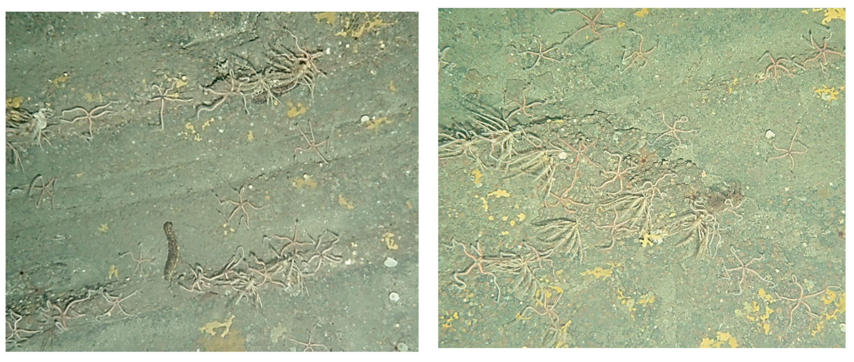
An example explained above is found in the results obtained in the analysis of significant environmental terrain variables in Zone 1 and 2 (localizations of ophiuroids and L. celtica, respectively). These species live in places with strong currents and in large aggregations. This behavior of living in dense patches maximizes their efficiency in the access to food as suspension feeders [65]. The results show that the positions chosen by the specimens of these species depend on the same environmental derivatives of the terrain (bpi, curvature and roughness), seeking maximum turbulence in the microscale range. This indicates that if two population groups of these species coincide in space, they will compete for the same locations since they have the same environmental preferences. This issue can be verified with images taken precisely in an area close to the study areas (between Zone 1 and Zone 2), where numerous specimens of these species can be found. Figure 16 shows the specimens of Ophiuroidea and L. celtica located on the same ground positions even when there are free parts of the sea floor.

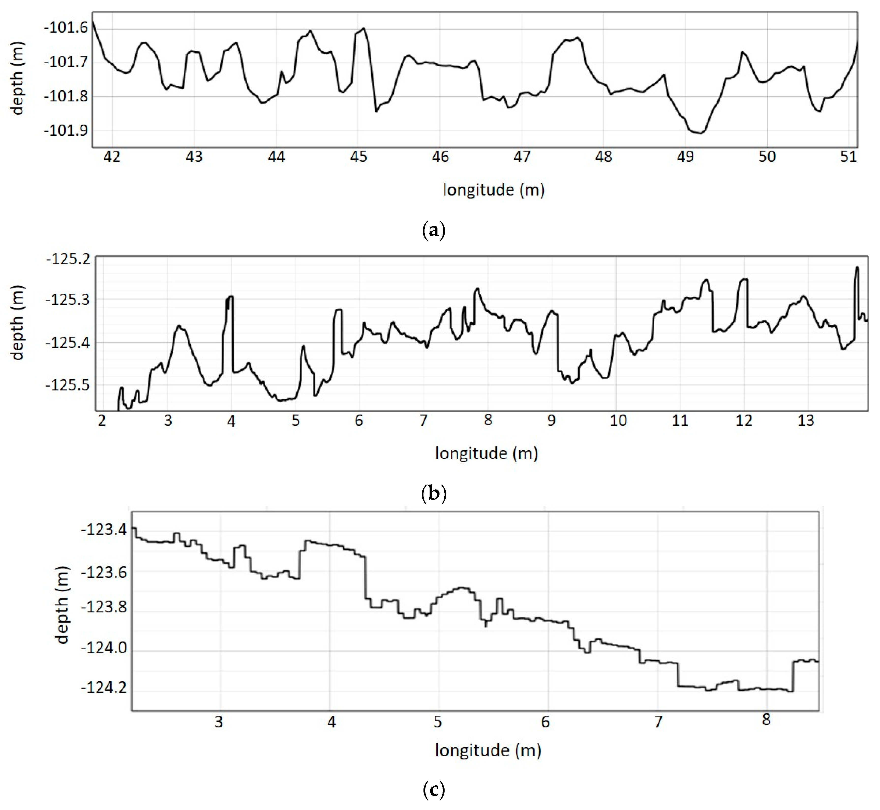
The dispersion of the specimens in Zones 1 and 2, through the Ripley’s K of these species, however, shows dissimilar results. The Ophiuroidea tend to form clusters of specimens when they are at distances greater than 13 cm (Figure 7a); roughly corresponding to the size of the specimens recorded in this study. However, the Crinoidea show a scattered distribution in the terrain in the range of scales studied (Figure 7b). This could be interpreted in L. celtica as behavior that minimizes competition between individuals related to food availability, since they are filter feeders. However, the spatial distribution of the Ophiuroidea, even when specimens of different species coexist, does not show any problem in sharing the same space. This behavior may be influenced by the lesser dependence of ophiuroids on water currents that carry organic matter, since a large proportion of their food is deposited or fixed in the ground

A. transiens was found forming dense aggregations always on rocky beds, in the Bay of Biscay and Northwest of Iberian Peninsula [3]. In the visual analysis of photographs, we can see that these small sponges are fixed to the flat faces of the stone blocks, seeking clear areas, but without large slopes or sudden changes (Figure 17). This coincides with the predictive analysis (Figure 12) in which the highest probability of occurrence was precisely in these places. Data on spatial distribution patterns in this case may be associated with the range of larvae with survival success and the distances to which they are fixed. According to the results of the Ripley’s K analysis, this maximum dispersion distance could be set at 1.5 m approx. Below this distance the specimens of this species show a distribution of groups.

D. cornigera, usually forming low patches with a mean size of about 30 cm. This species is colonial, forming three-dimensional structures growing by extra-tentacular budding on hard bottoms. Typically, it has a small and bushy colony with sparse irregular branching [66]. Among the environmental preferences that influence its location, the roughness of the terrain stands out. This can be mainly attributed to their diet, based on the capture of zooplankton present in the water, therefore choosing areas of greater turbulence and resuspension of food. Visually, the images show how the colonies are usually arranged on the edges of the stone blocks, fixing their base on them and extending the polyps towards the clearest areas (Figure 15). This same behavior in location preferences is reflected in the habitat suitability map (Figure 13).

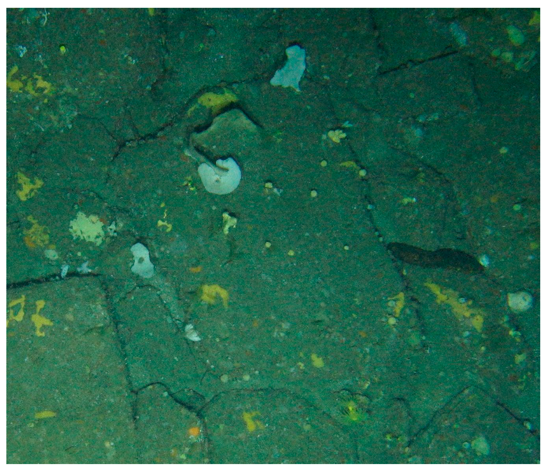
In the Bay of Biscay, P. ventilabrum was found forming small cups or funnels with thin walls and a short peduncle on rock ridges and outcrops. At the microscale range, the environmental preferences of this species focus mainly on roughness and both in the images and in the habitat suitability model (Figure 14), a distribution very similar to D. cornigera can be seen, although unlike the latter, BPI is not among its restrictions and it can be found both on edges with a clear horizon and on sunken rock edges.

4.3. Implementation of Deep-Learning Techniques to Annotate Benthic Species in Images

In all habitat predictive models, it is necessary to incorporate biologic information in order to create a benthic habitat map. Habitat predictive models require a representative number of geographic locations of specimens of the different species [39]. The automation of the image annotation process is, in fact, one of the clearest requirements of researchers and one of the issues that will enable underwater investigation of the benthos to take a further step forward.

From the above-described automatic detection algorithm using the trained network, it is possible to get the location of every individual over the orthomosaic, even with geographic coordinates. This information could then directly feed the microhabitat predictive models. Moreover, this approach can contribute to automate generation of density maps of selected species.

Although the performance of the YOLO v4 deep learning network after training with our custom dataset is similar to other object detection networks reported in the literature, there is room for improvement of the merit figures. In future works, we plan to improve our dataset with more annotated images and use different detection threshold for each specie, which we hope will improve the detection of small species such as A. transiens. The careful choosing of the overlap threshold of the non max suppression algorithm should also help with the correct identification of specimens in D. cornigera colonies. Additionally, we plan to train the network with all the species found in Zones 1, 2 and 3, so the algorithm could be used in more diverse areas.

5. Conclusions

We provided evidence that using a SfM approach and terrain-derived variables at centimetric scales, predictive microhabitat models can be designed with very high confidence levels. A 3D reconstruction model of a circalittoral rock area of a portion of the Bay of Biscay continental shelf enabled the characterization of some habitats in circalittoral rocky zones, extracting terrain variables from 3D model to find the principal factors that explain species location. These models enable the advance in knowledge about the factors that affect the space distribution among specimens of different or the same species at very fine scales.

The accurate classification of benthic habitats in circalittoral ecosystems is essential for developing realistic management strategies. However, automatic or semiautomatic approaches for deriving species identification, localization and quantification from underwater images are still scarce. The deep-learning-based approach presented here for the automatic annotation of images is very promising.