Regional Precipitation Model Based on Geographically and Temporally Weighted Regression Kriging


Abstract
:1. Introduction
2. Materials and Methods
2.1. Methodology
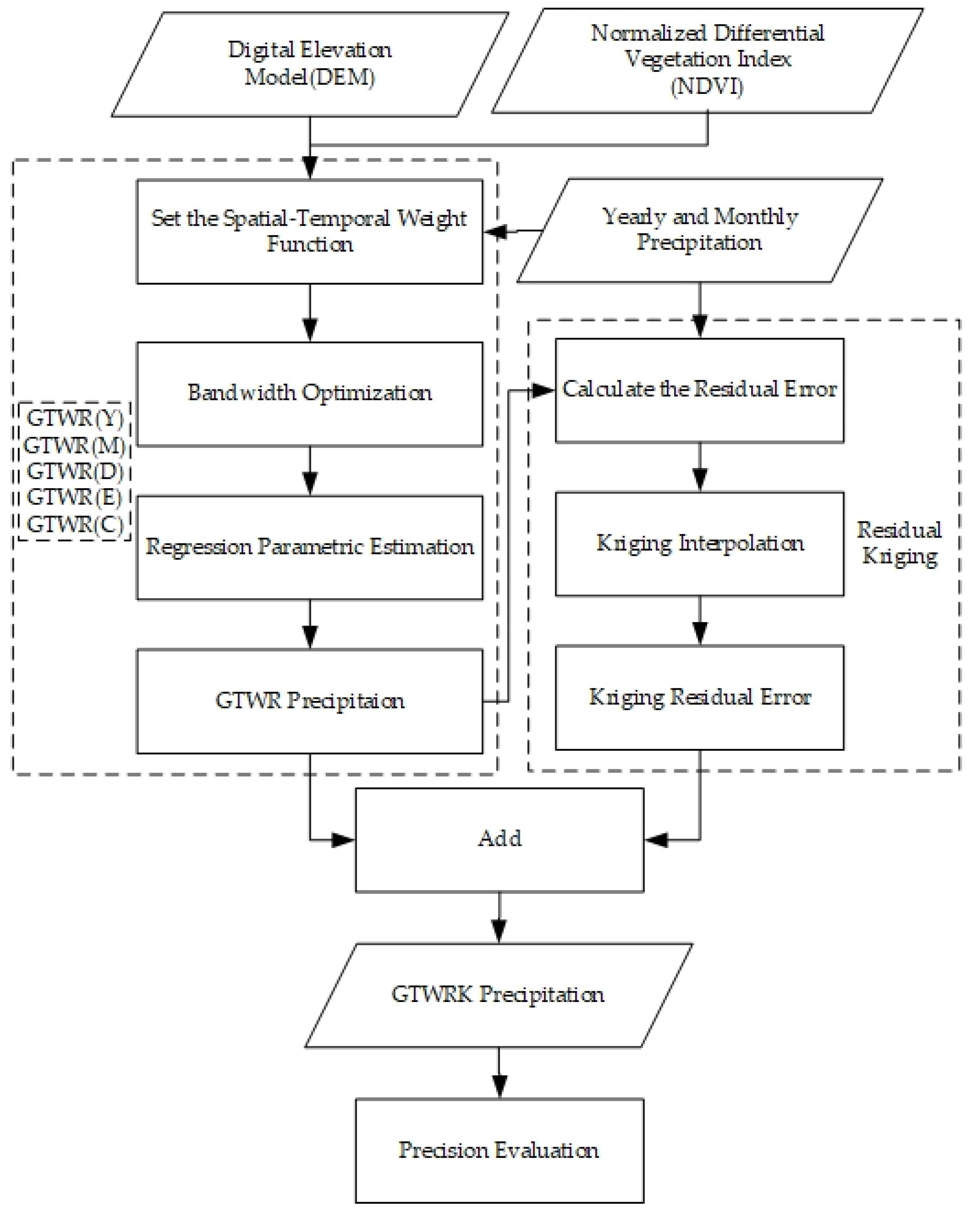
2.1.1. Geographically and Temporally Weighted Regression Model
2.1.2. Comparison Models with Different Spatial–Temporal Parameters
2.1.3. Geographically and Temporally Weighted Regression Kriging
2.1.4. Precision Evaluation
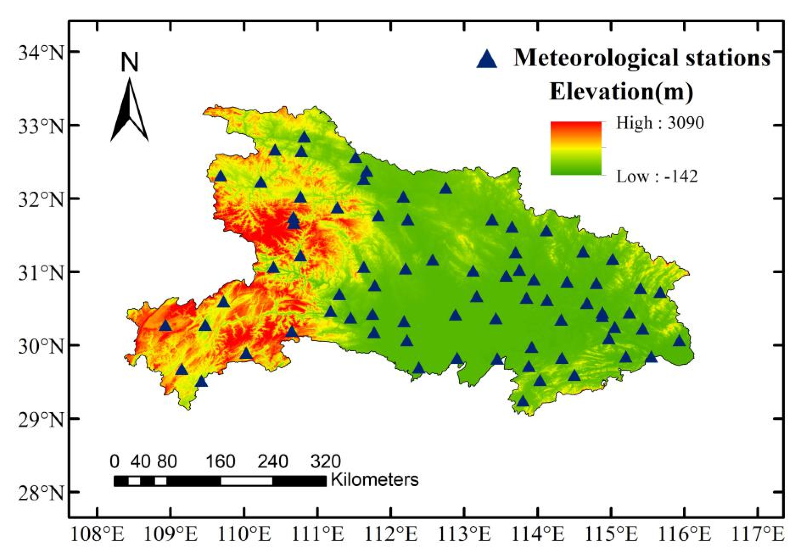
2.2. Study Area and Data
2.3. Data Preprocessing
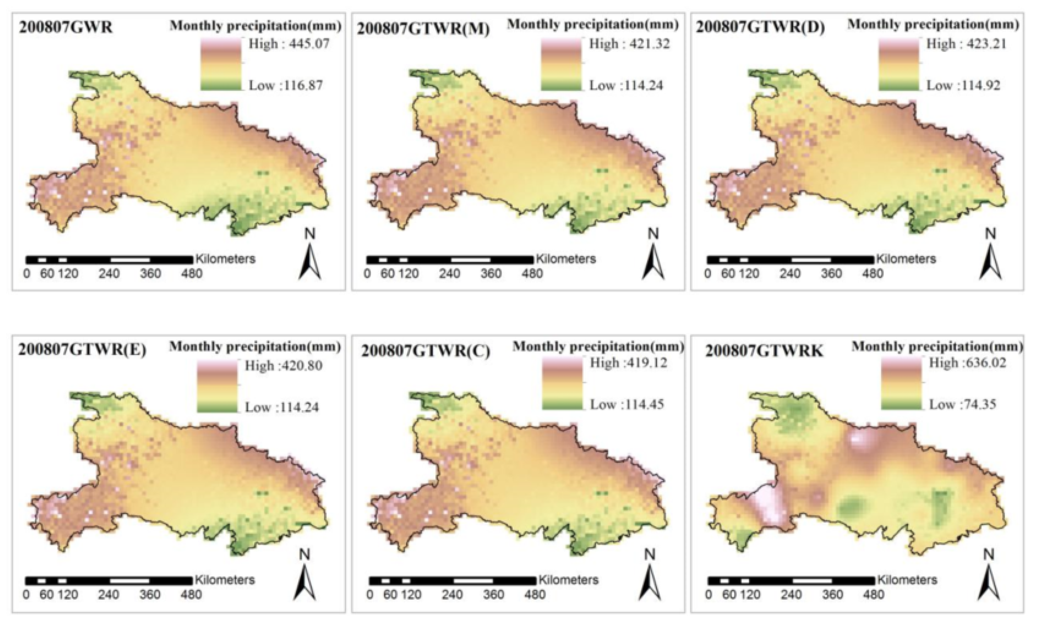
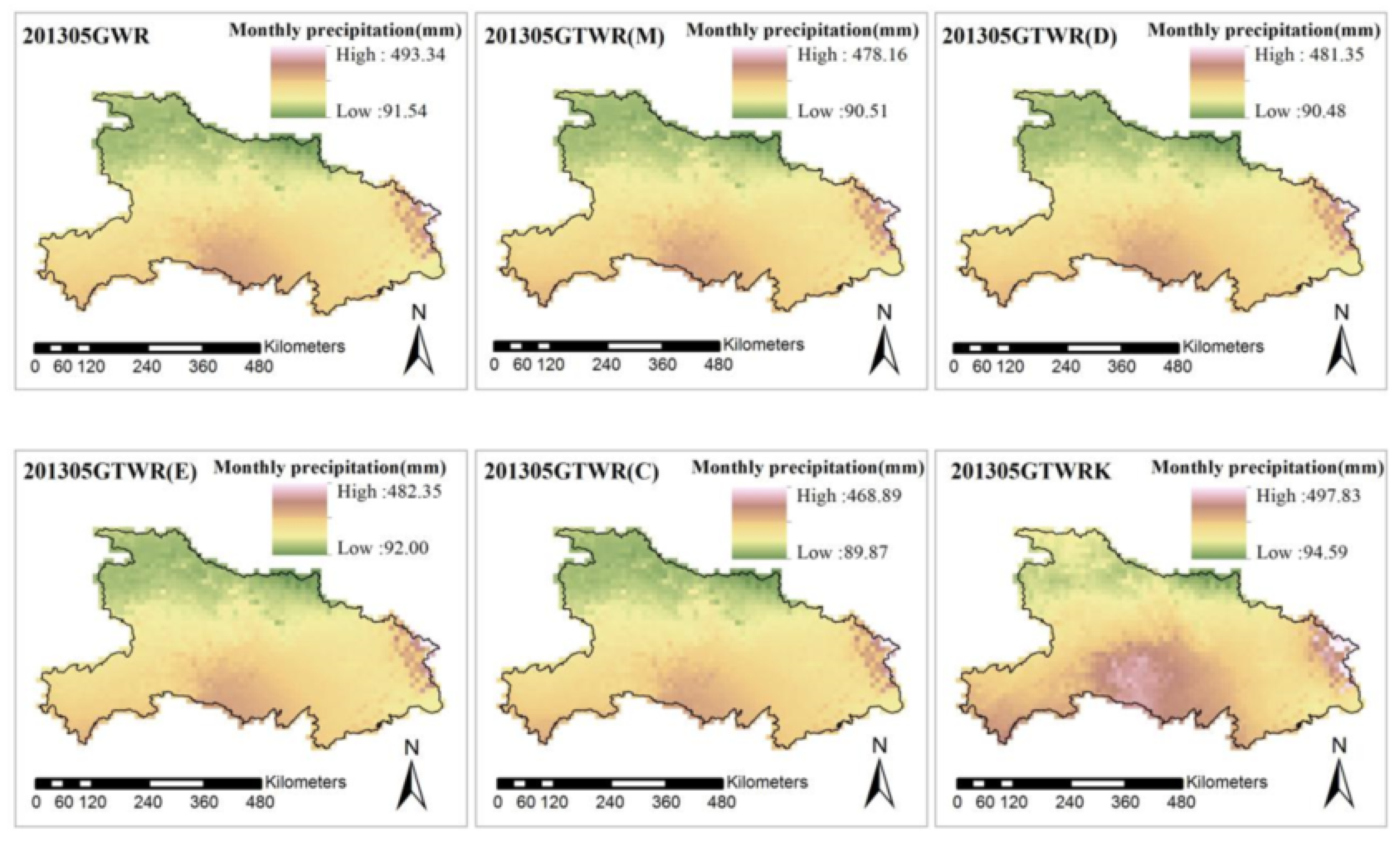
3. Results and Analysis
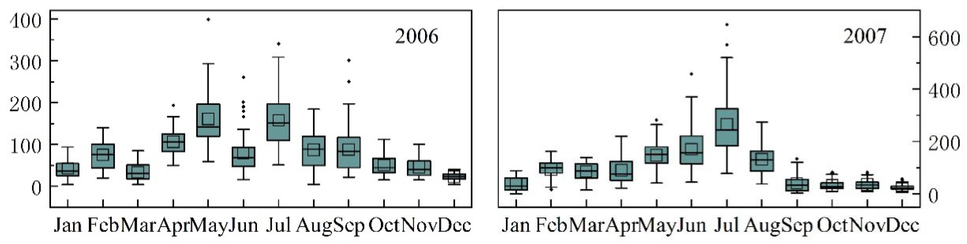
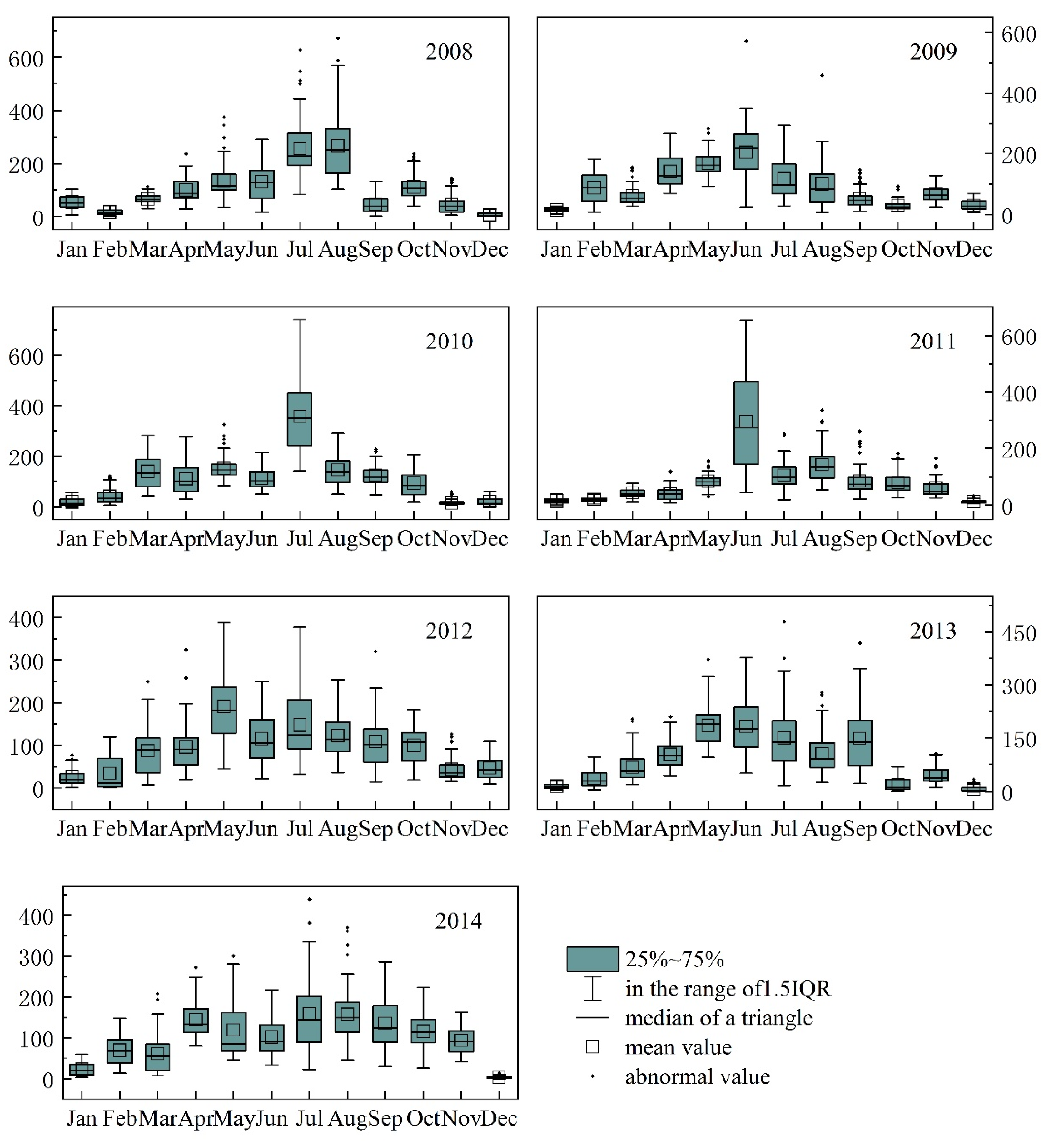
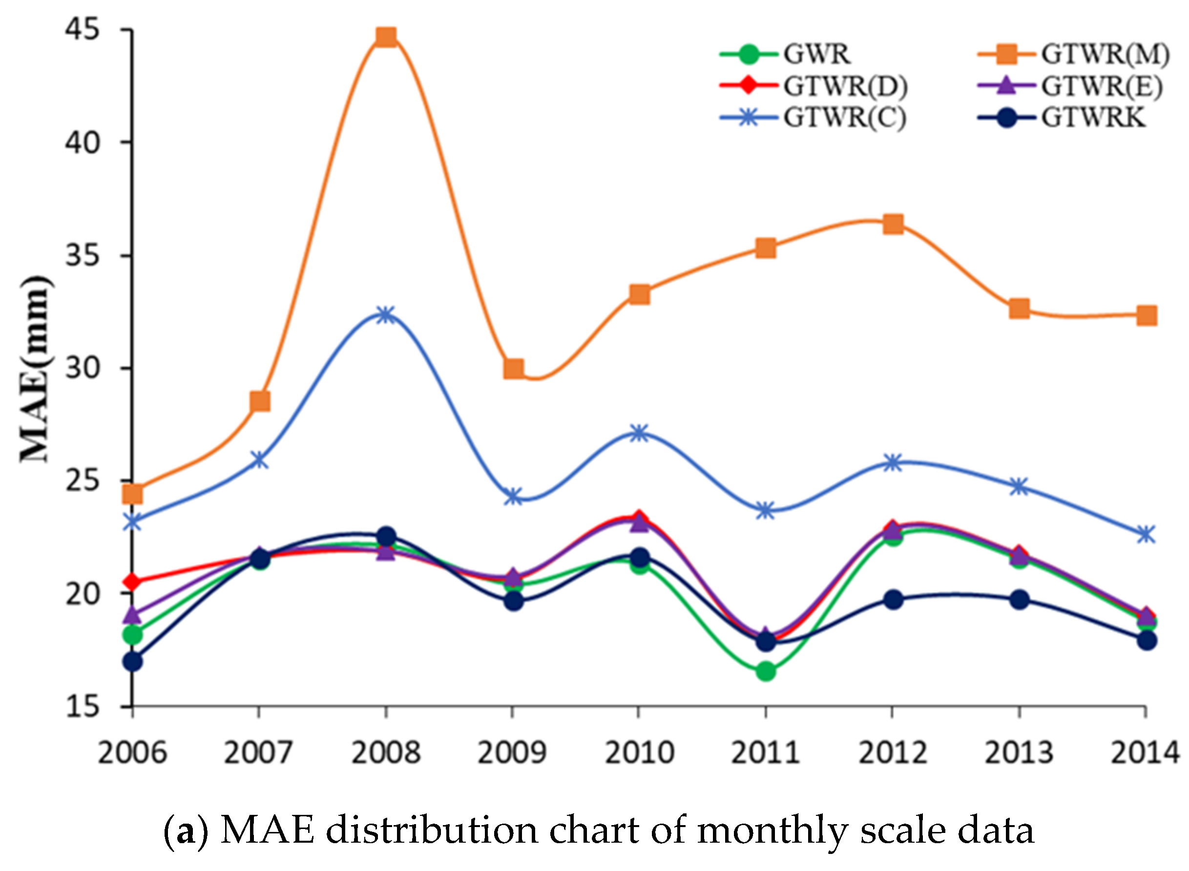
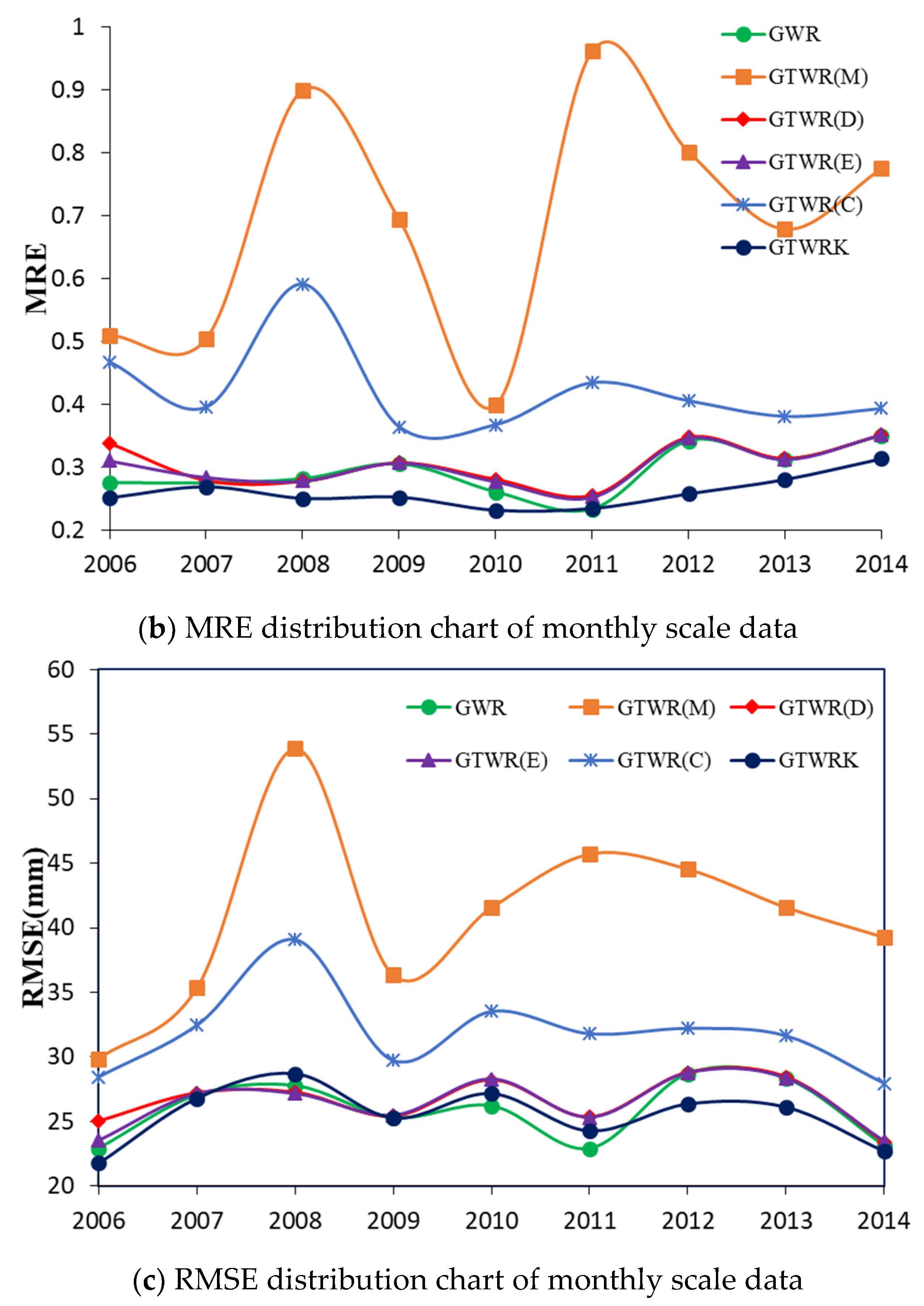
3.1. Monthly Data
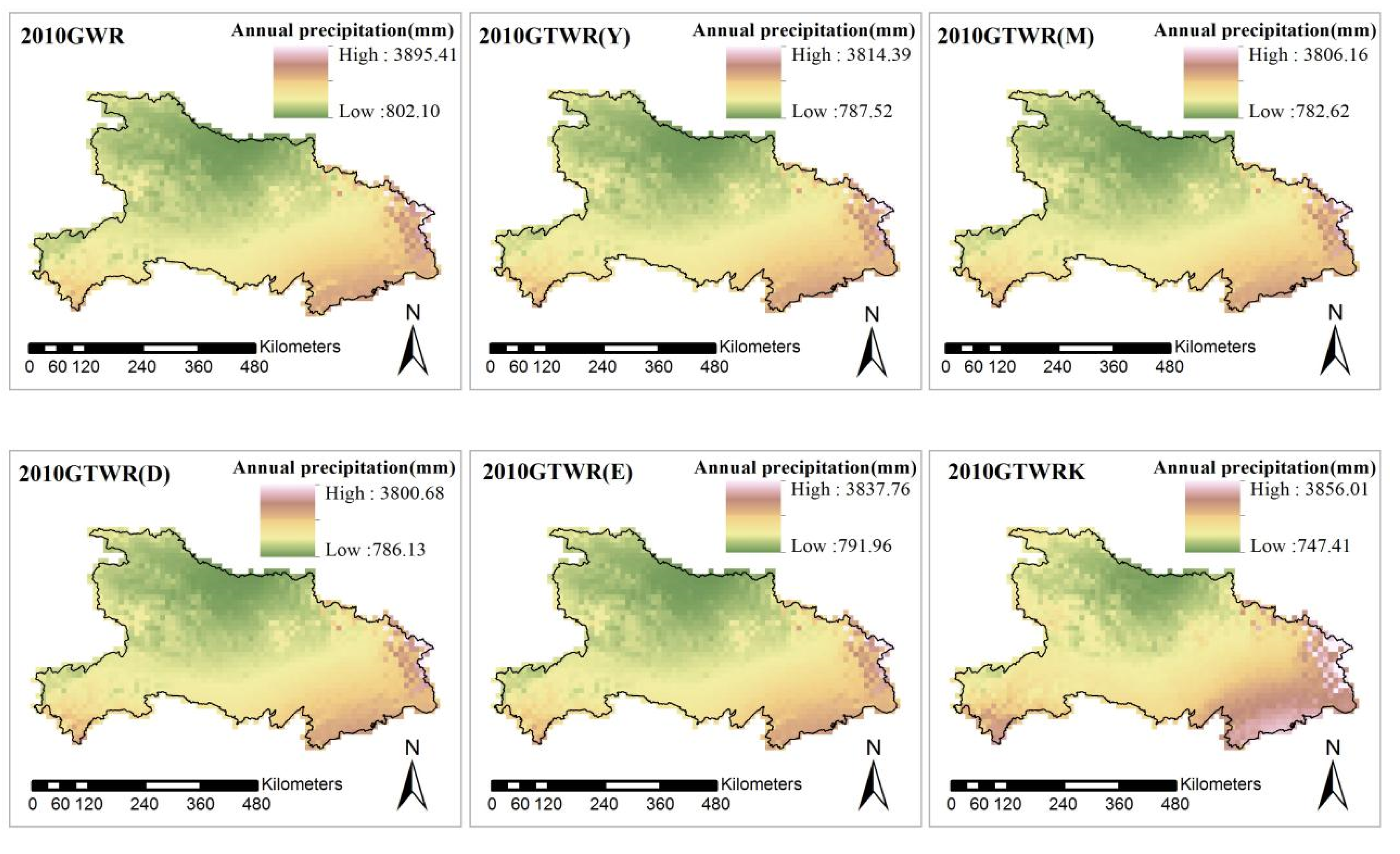
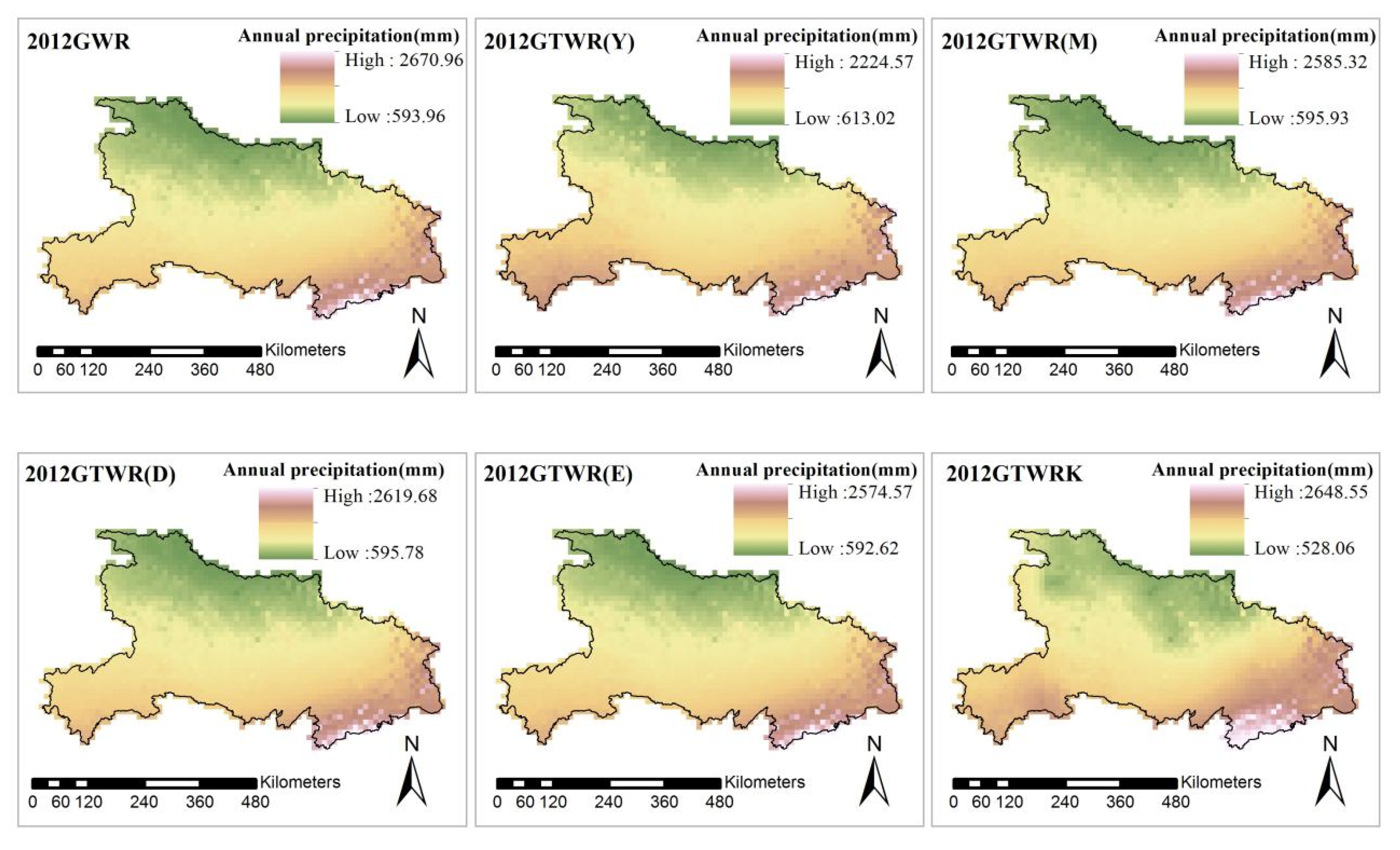
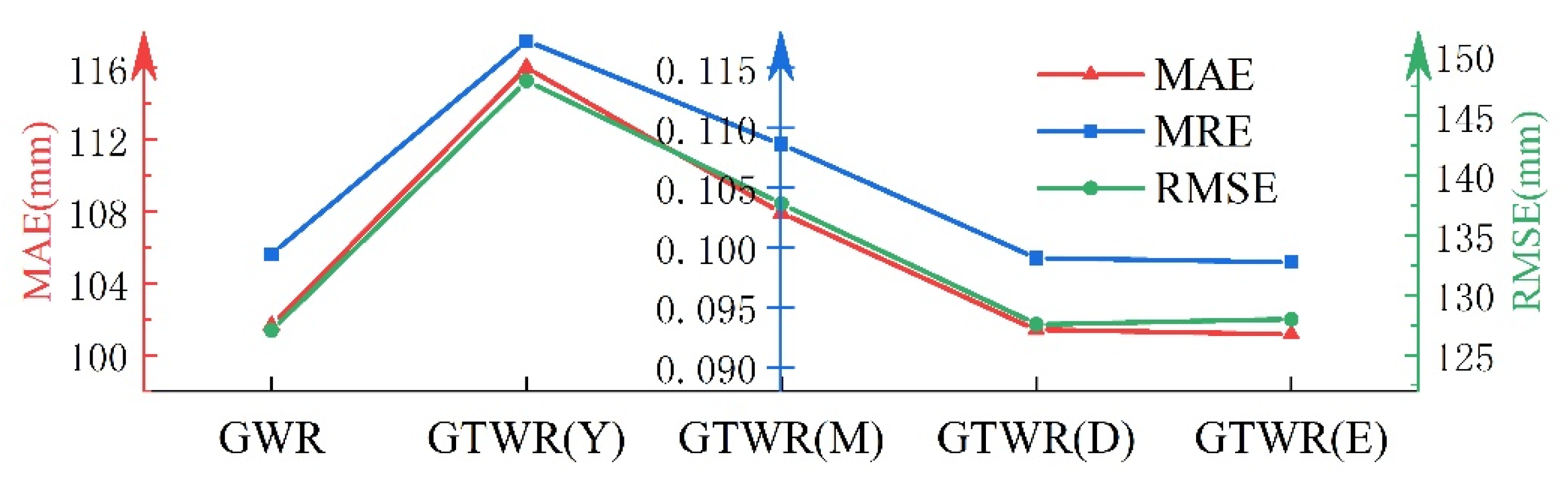
3.2. Annual Data
4. Discussion
5. Conclusions
- (1)
- GTWRK obtains a better average interpolation accuracy, compared to the GWR model. In the comparison between the GTWRK and GWR, the MAE decreased from 101.64 to 98.27. Consequently, we conclude that it is an improvement to extend GTWR with kriging.
- (2)
- The optimal timescale for interpolating precipitation data with the GTWR model is daily. The fitting accuracy is improved when the timescale is converted from yearly to daily. Compared with the GTWR(M) model, the average MAE, MRE, and RMSE of the monthly scale data decreased by 36%, 56%, and 35%, respectively, when using daily data. The same indices for the annual data reduced by 13%, 15%, and 14% when using daily data, respectively.
- (3)
- The temporal weight based on an exponential function improved the GTWR model at the monthly and annual data. It reduced the accuracy difference of the monthly scale between GTWR and GWR by about 3%. For the yearly scale data, the years with improved accuracy account for about 55%. Especially in 2008, 2009, 2010, 2011, and 2013, the accuracy was improved significantly. Meanwhile, the GTWRK improves the accuracy as measured by the MAE, MRE, and RMSE by 3%, 10%, and 1%, respectively, of monthly precipitation prediction, and by 3%, 10%, and 5%, respectively, of annual precipitation predictions.
- (4)
- The proposed model could be applied to manage similar phenomena with a large historical dataset. Meanwhile, the GTWR model takes into account the spatial and temporal heterogeneity of precipitation and produces better estimates of the residuals.
- (5)
- This work explored the annual, monthly, and daily scales to adjust the optimal time scale, while other time scales should be explored in future work. Additionally, the influence of the periodic characteristics of precipitation on the GTWR model needs further study.
Author Contributions
Funding
Conflicts of Interest
References
- Bhattacharya, A.; Adhikari, A.; Maitra, A. Multi-technique observations on precipitation and other related phenomena during cyclone Aila at a tropical location. Int. J. Remote Sens. 2013, 34, 1965–1980. [Google Scholar] [CrossRef]
- Goovaerts, P. Geostatistical approaches for incorporating elevation into the spatial interpolation of rainfall. J. Hydrol. 2000, 228, 113–129. [Google Scholar] [CrossRef]
- Vicente-Serrano, S.M.; Beguería, S.; López-Moreno, J.I. A multiscalar drought index sensitive to global warming: The standardized precipitation evapotranspiration index. J. Clim. 2010, 23, 1696–1718. [Google Scholar] [CrossRef] [Green Version]
- Plouffe, C.C.F.; Robertson, C.; Chandrapala, L. Comparing interpolation techniques for monthly rainfall mapping using multiple evaluation criteria and auxiliary data sources: A case study of Sri Lanka. Environ. Model. Softw. 2015, 67, 57–71. [Google Scholar] [CrossRef]
- Collischonn, B.; Collischonn, W.; Tucci, C.E.M. Daily hydrological modeling in the Amazon basin using TRMM rainfall estimates. J. Hydrol. 2008, 360, 207–216. [Google Scholar] [CrossRef]
- Lin, Z.; Mo, X.; Li, H.; Li, H. Comparison of Three Spatial Interpolation Methods for Climate Variables in China. Acta Geogr. Sin. 2002, 57, 47–56. [Google Scholar]
- Feng, Z.; Yang, Y.; Ding, X.; Lin, Z. Optimization of the spatiaI interpolation methods for climate resources. Geogr. Res. 2004, 23, 357–364. [Google Scholar]
- Liu, J.-F.; Chen, R.-S.; Han, C.-T.; Tan, C.-P. Evaluating TRMM multi-satellite precipitation analysis using gauge precipitation and MODIS snow-cover products. Adv. Water Sci. 2010, 21, 343–348. [Google Scholar]
- Zhu, L.; Huang, J. Comparis on of spatial interpolation m ethod for precipitation of mountain areas in county scale. Trans. CSAE 2007, 23, 80–85. [Google Scholar]
- Li, C.; Chen, L.; Wang, Y. Research on spatial interpolation of rainfall distribution-A case study of Idaho State in the USA. Miner. Resour. Geol. 2007, 21, 684–687. [Google Scholar]
- Lam, N.S.-N. Spatial Interpolation Methods: A Review. Am. Cartogr. 1983, 10, 129–150. [Google Scholar] [CrossRef]
- Li, L.; Revesz, P. Interpolation methods for spatio-temporal geographic data. Comput. Environ. Urban. Syst. 2004, 28, 201–227. [Google Scholar] [CrossRef]
- Peng, S. Developments of Spatio-temporal Interpolation Methods for Meteorological Elements. Master’s Thesis, Central South University, Changsha, China, 2010. [Google Scholar]
- Li, S.; Shu, H.; Xu, Z. Interpolation of temperature based on spatial-temporal Kriging. Geomatics Inf. Sci. Wuhan Univ. 2012, 37, 237–241. [Google Scholar]
- Lu, Y. Spatio-Temporal Cokriging Interpolation for Air Pollution Index Analysis. Master’s Thesis, Chinese Academy of Surveying & Mapping, Beijing, China, 2018. [Google Scholar]
- Fotheringham, A.S.; Brunsdon, C.; Charlton, M.E. Geographically Weighted Regression: A Method for Exploring Spatial Nonstationarity. Geogr. Anal. 1996, 28, 281–298. [Google Scholar]
- Hu, Q.; Li, Z.; Wang, L.; Huang, Y.; Wang, Y.; Li, L. Rainfall Spatial Estimations: A Review from Spatial Interpolation to Multi-Source Data Merging. Water 2019, 11, 579. [Google Scholar] [CrossRef] [Green Version]
- Wang, M.; He, G.; Zhang, Z.; Wang, G.; Zhang, Z.; Cao, X.; Wu, Z.; Liu, X. Comparison of Spatial Interpolation and Regression Analysis Models for an Estimation of Monthly Near Surface Air Temperature in China. Remote. Sens. 2017, 9, 1278. [Google Scholar] [CrossRef] [Green Version]
- Huang, B.; Wu, B.; Barry, M. Geographically and temporally weighted regression for modeling spatio-temporal variation in house prices. Int. J. Geogr. Inf. Sci. 2010, 24, 383–401. [Google Scholar] [CrossRef]
- Wu, B.; Li, R.; Huang, B. A geographically and temporally weighted autoregressive model with application to housing prices. Int. J. Geogr. Inf. Sci. 2014, 28, 1186–1204. [Google Scholar] [CrossRef]
- Fotheringham, A.S.; Crespo, R.; Yao, J. Geographical and Temporal Weighted Regression (GTWR). Geogr. Anal. 2015, 47, 431–452. [Google Scholar] [CrossRef] [Green Version]
- Xiao, H.; Yi, D. Empirical study of carbon emission drivers based on Geographically time weighted regression model. Stat. Inf. Forum 2014, 29, 83–89. [Google Scholar]
- Liu, J.; Yang, Y.; Xu, S.; Zhao, Y.; Wang, Y.; Zhang, F. A geographically temporal weighted regression approach with travel distance for house price estimation. Entropy 2016, 18, 303. [Google Scholar] [CrossRef]
- Song, C.; Kwan, M.P.; Zhu, J. Modeling fire occurrence at the city scale: A comparison between geographically weighted regression and global linear regression. Int. J. Environ. Res. Public Health 2017, 14, 396. [Google Scholar] [CrossRef] [PubMed] [Green Version]
- Zhou, Y.; Wu, L.; Zhang, Y.; Shen, Y.; Qin, K.; Bai, Y. A Geographically and Temporally Weighted Regression Model for Ground-Level PM2.5 Estimation from Satellite-Derived 500 m Resolution AOD. Remote Sens. 2016, 8, 262. [Google Scholar]
- Qin, K.; Rao, L.; Xu, J.; Bai, Y.; Zou, J.; Hao, N.; Li, S.; Yu, C. Estimating ground level NO2 concentrations over central-eastern China using a satellite-based geographically and temporally weighted regression model. Remote Sens. 2017, 9, 950. [Google Scholar] [CrossRef] [Green Version]
- Wei, Q.; Zhang, L.; Duan, W.; Zhen, Z. Global and Geographically and Temporally Weighted Regression Models for Modeling PM2.5 in Heilongjiang, China from 2015 to 2018. Int. J. Environ. Res. Public Health 2019, 16, 5107. [Google Scholar] [CrossRef] [PubMed] [Green Version]
- Brunsdon, C.; McClatchey, J.; Unwin, D.J. Spatial variations in the average rainfall-altitude relationship in Great Britain: An approach using geographically weighted regression. Int. J. Climatol. 2001, 21, 455–466. [Google Scholar] [CrossRef] [Green Version]
- Chen, C.; Zhao, S.; Duan, Z.; Qin, Z. An Improved Spatial Downscaling Procedure for TRMM 3B43 Precipitation Product Using Geographically Weighted Regression. IEEE J. Sel. Top. Appl. Earth Obs. Remote Sens. 2015, 8, 4592–4604. [Google Scholar] [CrossRef]
- Lv, A.; Zhou, L. A rainfall model based on a Geographically Weighted Regression algorithm for rainfall estimations over the arid Qaidam Basin in China. Remote Sens. 2016, 8, 311. [Google Scholar] [CrossRef] [Green Version]
- Georganos, S.; Abdi, A.M.; Tenenbaum, D.E.; Kalogirou, S. Examining the NDVI-rainfall relationship in the semi-arid Sahel using geographically weighted regression. J. Arid Environ. 2017, 146, 64–74. [Google Scholar] [CrossRef]
- Li, Y.; Xiong, L.; Yan, L.A. Geographically Weighted Regression Krigin Approach for TRMM-Rain Gauge Data Merging and its Application in Hydrological Forecasting. Resour. Environ. Yangtze Basin 2017, 26, 1359–1368. [Google Scholar]
- Liu, J.; Zhao, Y.; Yang, Y.; Xu, S.; Zhang, F.; Zhang, X.; Shi, L.; Qiu, A. A mixed geographically and temporallyweighted regression: Exploring spatial-temporal variations from global and local perspectives. Entropy 2017, 19, 53. [Google Scholar] [CrossRef] [Green Version]
- Tobler, W. A computer movie simulating urban growth in the Detroit region. Econ. Geogr. 1970, 46 (Suppl. 46), 234–240. [Google Scholar] [CrossRef]
- Ge, L.; Zhao, Y.; Sheng, Z.; Wang, N.; Zhou, K.; Mu, X.; Guo, L.; Wang, T.; Yang, Z.; Huo, X. Construction of a seasonal difference-geographically and temporally weighted regression (SD-GTWR) model and comparative analysis with GWR-based models for hemorrhagic fever with renal syndrome (HFRS) in Hubei Province (China). Int. J. Environ. Res. Public Health 2016, 13, 1062. [Google Scholar] [CrossRef] [PubMed] [Green Version]
- Du, Z.; Wu, S.; Zhang, F.; Liu, R.; Zhou, Y. Extending geographically and temporally weighted regression to account for both spatiotemporal heterogeneity and seasonal variations in coastal seas. Ecol. Inform. 2018, 43, 185–199. [Google Scholar] [CrossRef]
- Dong, F.; Wang, Y.; Zhang, X. Can Environmental Quality Improvement and Emission Reduction Targets Be Realized Simultaneously? Evidence from China and A Geographically and Temporally Weighted Regression Model. Int. J. Environ. Res. Public Health 2018, 15, 2343. [Google Scholar] [CrossRef] [PubMed] [Green Version]
- Qin, W. The Basic Theoretics and Application Research on Geographically Weighted Regression. Ph.D. Thesis, Tongji University, Shanghai, China, 2007. [Google Scholar]
- Yuan, M. Dynamic Change of Vegetation and Phenology Response to Climate Change in Hubei Province. Master’s Thesis, Wuhan University, Wuhan, China, 2017. [Google Scholar]
- Spreen, W.C. A determination of the effect of topography upon precipitation. Trans. Am. Geophys. Union 1947, 28, 285–290. [Google Scholar] [CrossRef]
- Smith, R.B. The influence of mountains on the atmosphere. Adv. Geophys. 1979, 21, 87–230. [Google Scholar]
- Kang, L.; Di, L.; Shao, Y.; Yu, E.; Zhang, B.; Shrestha, R. Study of the NDVI-precipitation correlation stratified by crop type and soil permeability. In Proceedings of the 2013 2nd International Conference on Agro-Geoinformatics: Information for Sustainable Agriculture, Agro-Geoinformatics, Fairfax, VA, USA, 12–16 August 2013; pp. 194–199. [Google Scholar]
- Feng, J.; Zhang, H.; Hu, X.; Shi, Q.; Zubaidai, M. Spatial non-stationarity characteristics of the impacts of precipitation and temperature on vegetation coverage index: A case study in Yili River Valley, Xinjiang. Acta Ecol. Sin. 2016, 36, 4626–4634. [Google Scholar]


| Model | Spatial Weight | Time Weight | Timescale | Calculation Method | Residual Processing |
|---|---|---|---|---|---|
| GTWR(Y) | Gaussian | Gaussian | Year | Subtraction | None |
| GTWR(M) | Gaussian | Gaussian | Month | Subtraction | None |
| GTWR(D) | Gaussian | Gaussian | Day | Subtraction | None |
| GTWR(E) | Gaussian | Exponential | Day | Subtraction | None |
| GTWR(C) | Gaussian | Exponential | Day | Sinusoidal | None |
| GTWRK | Gaussian | Exponential | Day | Subtraction | Kriging interpolation |
| Model | MAE (mm) | MRE | RMSE (mm) |
|---|---|---|---|
| GWR | 20.36 | 0.29 | 25.80 |
| GTWR(M) | 33.08 | 0.69 | 40.90 |
| GTWR(D) | 21.09 | 0.31 | 26.57 |
| GTWR(E) | 20.92 | 0.30 | 26.40 |
| GTWR(C) | 25.54 | 0.42 | 31.88 |
| GTWRK | 19.77 | 0.26 | 25.47 |
| Model | MAE (mm) | MRE | RMSE (mm) |
|---|---|---|---|
| GWR | 101.64 | 0.10 | 127.08 |
| GTWR(Y) | 116.04 | 0.12 | 147.94 |
| GTWR(M) | 107.93 | 0.11 | 137.69 |
| GTWR(D) | 101.41 | 0.10 | 127.57 |
| GTWR(E) | 101.17 | 0.10 | 128.01 |
| GTWRK | 98.27 | 0.09 | 120.60 |
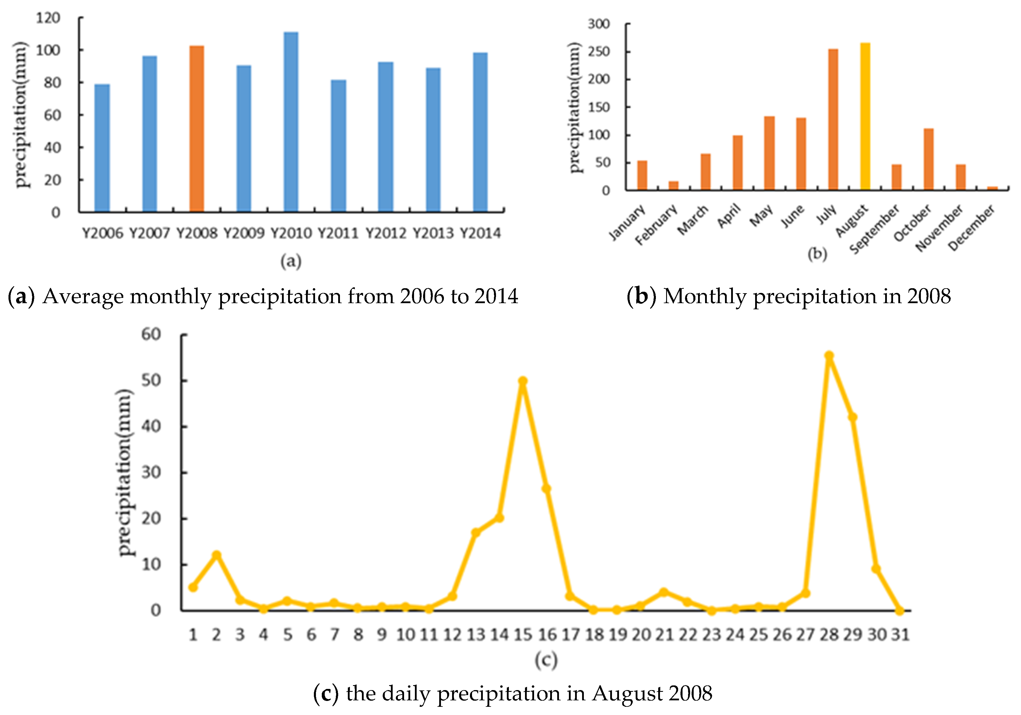
| Month | Kolmogorov-Smirnova | Kurtosis | Skewness | Average Precipitation (mm) | |
|---|---|---|---|---|---|
| df | Sig. | ||||
| January | 60 | 0.200 * | 0.674 | 0.553 | 53.99 |
| February | 60 | 0.200 * | −0.424 | −0.01 | 16.29 |
| March | 60 | 0.200 * | 1.228 | 0.448 | 65.99 |
| April | 60 | 0.200 * | 5.968 | 1.661 | 99.41 |
| May | 60 | 0.005 | 3.979 | 1.802 | 134.22 |
| June | 60 | 0.006 | −0.139 | 0.844 | 130.83 |
| July | 60 | 0.059 | 0.95 | 0.939 | 255.36 |
| August | 60 | 0.054 | 0.922 | 0.886 | 266.10 |
| September | 60 | 0.039 | 0.342 | 0.626 | 46.81 |
| October | 60 | 0.200 * | 0.965 | 0.273 | 111.70 |
| November | 60 | 0.200 * | 0.471 | −0.08 | 46.72 |
| December | 60 | 0 | 0.709 | 0.386 | 7.01 |
© 2020 by the authors. Licensee MDPI, Basel, Switzerland. This article is an open access article distributed under the terms and conditions of the Creative Commons Attribution (CC BY) license (http://creativecommons.org/licenses/by/4.0/).
Share and Cite
Zhang, W.; Liu, D.; Zheng, S.; Liu, S.; Loáiciga, H.A.; Li, W. Regional Precipitation Model Based on Geographically and Temporally Weighted Regression Kriging. Remote Sens. 2020, 12, 2547. https://doi.org/10.3390/rs12162547
Zhang W, Liu D, Zheng S, Liu S, Loáiciga HA, Li W. Regional Precipitation Model Based on Geographically and Temporally Weighted Regression Kriging. Remote Sensing. 2020; 12(16):2547. https://doi.org/10.3390/rs12162547
Chicago/Turabian StyleZhang, Wei, Dan Liu, Shengjie Zheng, Shuya Liu, Hugo A. Loáiciga, and Wenkai Li. 2020. "Regional Precipitation Model Based on Geographically and Temporally Weighted Regression Kriging" Remote Sensing 12, no. 16: 2547. https://doi.org/10.3390/rs12162547