A Method to Automatically Detect Changes in Multitemporal Spectral Indices: Application to Natural Disaster Damage Assessment

Abstract

This paper presents a new method, based on clustering and thresholding, to automatically perform binary change detection in multitemporal spectral indices. The method is denoted as Buffer-From-Cluster Approach (BFCA). To estimate the distributions of changed and unchanged pixels, as needed for the purpose of a reliable thresholding of a spectral index, a clustering algorithm is preliminarily applied to identify image objects possibly corresponding to areas where significant changes occurred. Then, a buffer zone is created around the selected cluster to identify unchanged areas surrounding changed ones. The cluster and the buffer zone are jointly analyzed to estimate the distributions of changed and unchanged pixels and to verify that they can be distinguished from each other. Finally, the results of thresholding and clustering are combined to generate the binary change map. The BFCA has been conceived to map the extent of the areas affected by a natural disaster like wildfire. To validate the proposed method, burned area maps produced by applying the BFCA to spectral indices derived from Sentinel-2 data have been compared to maps produced by the Copernicus Emergency Management Service. For testing the multi-hazard detection capability, the same kind of exercise has been carried out for a flooding test case too. The positive results of the comparison have confirmed the effectiveness of the proposed method.

1. Introduction

The frequency and the destructivity of natural hazards is continuously increasing. They leave in their wake a trail of injury, death, loss of livestock, property damage, and economic loss. This implies the need for improving the capability to manage these events. The availability of a synoptic map of the affected area in a short time strongly supports a rapid response to natural disasters [1]. Satellite earth observation (EO) data represent the most useful source of information to quickly map the extension of the area affected by a natural hazard [2].

Operational services like the rapid mapping component of the Copernicus Emergency Management Service (CEMS) currently provide emergency managers with maps of natural disasters at different spatial resolutions depending on the kind of EO data used to produce the maps. CEMS is an on-demand service, being triggered on request by authorized users (e.g., National Civil Protection Agencies), which is often at least partially based on the visual interpretation of a skilled operator. However, the present availability of Sentinel-1/2/3 data allows for routinely producing maps of areas affected by disasters (without the need of waiting for an activation). An unsupervised, fully automatic algorithm able to rapidly map the disaster’s extent is needed to accomplish this routine production, especially if many EO data must be sequentially processed (e.g., when working at large spatial scales).

Change detection aiming at producing binary maps where changed and unchanged areas are separated, often denoted as binary change detection [3], represents the most commonly used technique for disaster extent assessment through EO data. It is usually applied using multitemporal satellite images. Several unsupervised binary change detection methods were developed in past studies including image differencing (mostly used for multispectral images) or ratioing (for SAR images) (e.g., [4,5]) principal components analysis (e.g., [6,7]), change vector analysis (e.g., [8,9]), and vegetation index differencing (e.g., [10]). In [3,11,12], thorough reviews of change detection techniques are provided.

Due to its simplicity, image (or vegetation index) differencing is a popular method for performing binary change detection. It only requires calculating the values of the difference between the corresponding pixels in two images. Basically, large values in the difference map indicate the occurrence of change. From the difference map, the binary map representing change/no-change classification is usually produced by thresholding the difference map at a determined value. The determination of the threshold value is often very critical, because too low a value may give rise to a binary map presenting many false alarms, while too high a value may suppress significant changes. The proper value of the threshold generally depends on many factors such as environmental and satellite system parameters, so that it can be highly variable. Therefore, thresholds derived in an empirical way may lack generality and their applicability to data acquired under different environmental conditions can be questioned, while determining thresholds through photointerpretation is not consistent with a routine production of many change maps.

To cope with the aforementioned problems, it is possible to rely on automatic thresholding. Several methods to automatically select a threshold are available in the literature (e.g., [13,14,15,16,17,18]). However, they generally assume that the histogram of the analyzed image is the mixture of two distributions: changed and unchanged pixels, in this case. Thus, the histogram should have two peaks and the population of changed pixels should be large enough to give rise to a significant statistical mode in the histogram. This happens if the spatial extent of the area affected by the change is not much smaller than the size of the image. Hence the idea, originally proposed in [4], to divide the considered image into a set of non-overlapping sub-images (or splits) and select the splits having a high probability to contain a significant amount of changed pixels. This technique is known as the split-based approach (SBA). The choice of the size of the sub-images is subjective and if no splits are selected, their size can be decreased to try to increase the percentage of changed pixels in the sub-images. Along this line, in [19], splits of various dimensions are sequentially analyzed to search for bimodal histograms. The analysis of a large number of splits might be time consuming if many images have to be processed, e.g., when working at large spatial scales, and/or when simultaneous observations of the same scene must be considered, e.g., when different bands (or combinations of bands) of a multispectral image have to be processed.

Thresholding can be applied in combination with other image segmentation techniques to deal with the uncertainties in the determination of the threshold. Within the framework of a region growing algorithm (RGA), the threshold is used to identify an initial seed region. Then, RGA analyses neighboring pixels of the seed points and determines whether the pixel neighbors should be added to the seed region based on a tolerance criterion [20,21]. RGA is applied to disaster damage mapping through change detection in several papers, for instance in [22,23,24] for burned area (BA) mapping and in [25,26] for flood mapping. Recently, cluster-based thresholds have been introduced. In [27], where BA maps are derived from MODIS highest resolution (250 m) data, active fire (hotspots) information, provided by the MODIS Global Monthly Fire Location Product (MCD14ML), is used to identify the clusters. Then, a threshold is computed by analyzing burned and unburned pixels from the vicinity of each cluster. A combination of clustering and thresholding is proposed in [22] as well. Both in [22] and in [27], thresholding is applied within the framework of a RGA.

In this paper, an innovative method to perform automatic change detection, aiming at mapping the extent of the area affected by a natural disaster, is presented. It will be indicated hereafter as “Buffer-From-Cluster Approach” (BFCA). The BFCA has been conceived to work with one, or more than one, multitemporal spectral index (difference between the corresponding pixels in two spectral index images). The use of more than one spectral index generally adds complementary information for the change detection task (e.g., [28]), thus likely improving the accuracy of the result of the BFCA.

The BFCA combines clustering, thresholding, and region growing. With respect to the approach proposed in [27], that has been specifically designed for BA mapping, the BFCA can be applied to map the extent of other kinds of disasters like floods. In addition, the BFCA does not need any information furnished by ancillary products and the thresholds discriminating changed and unchanged pixels are determined using one of the automatic thresholding algorithms available in the literature [14]. With respect to the processor designed in [24] for AVHRR data, which uses the thresholding method developed in [14] and the RGA, the BFCA estimates the distribution functions representing changed and unchanged pixels to reliably apply automatic thresholding. In the processing chain designed in [22], which combines clustering, thresholding and region growing, a SBA similar to that proposed in [4,15] is used to determine the threshold. Conversely, the BFCA directly analyzes portions of an image of a multitemporal spectral index (MTSI) that likely contains comparable amounts of changed and unchanged pixels.

Burned area mapping has been chosen as main application of the BFCA and, to assess the aforementioned possibility to apply it even to other kinds of natural disasters, flood mapping has been tested as well. In both cases, Sentinel-2 (S2) data have been used to derive the MTSIs. This paper describes the various phases of the BFCA and presents the results of its application to S2-derived MTSIs useful to map BAs and floods. Validation has been accomplished by comparing the BFCA-derived maps to maps produced by the CEMS in the period 2018–2020, which have been therefore considered as the benchmark.

2. Materials and Methods

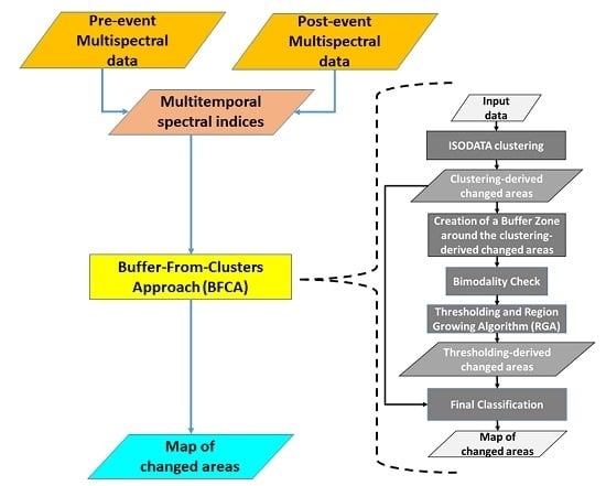
2.1. The Buffer-From-Cluster Approach

The flowchart of the new BFCA is shown in Figure 1. Each operation will be described in detail hereafter.

2.1.1. Clustering and Creation of the Buffer Zone

The first step of the BFCA consists of the application of the Iterative Self-Organizing Data Analysis Technique Algorithm (ISODATA) to the input data. The ISODATA is an unsupervised clustering algorithm that separates groups of objects in a scene. A typical scene consists of regular and/or irregular regions arranged in a patchwork manner, each containing one class of surface cover type (e.g., burned or flooded areas, croplands, forests, manmade structures, etc.). These homogeneous regions are the objects in the scene. Objects within each cluster should be as close to each other as possible and as far from other objects in other clusters as possible. The ISODATA begins with arbitrary cluster means and then clusters the pixels according to the minimum spectral distance technique. It is an iterative procedure, in which each iteration recalculates means and reclassifies pixels with respect to the new means. The process ends when a maximum number of iterations has been performed, or a maximum percentage of unchanged pixels between two iterations has been reached. The ISODATA does not keep a fixed number of clusters. In particular, clusters having a very large number of members are split, while if two cluster means are very close in terms of spectral distance (e.g., they represent an unnecessary or an injudicious division of the data), they are merged [29]. Clusters that contain so few points as to be meaningless (e.g., that they would not give acceptable statistics estimates if used in training a maximum likelihood classifier) are discarded and their members are reassigned to other clusters.

Since the ISODATA splits and merges clusters, it just requires specifying a range for the number of clusters. The optimum number of clusters is not known, so it is generally chosen to be conservatively high [29]. Hence, although here the goal is to distinguish changed pixels from unchanged ones, a maximum number of 10 clusters has been chosen as done in [22]. In Section 4.3, the impact of this choice on the BFCA-derived maps will be analyzed. A cluster can be considered as a sort of unknown class of surface cover type, and it is the task of the user to label the classes after the application of the clustering [29].

Let us assume that we are searching for positive values of the considered MTSI, that is, we are searching for significant increases of the spectral index. In this case, the objects belonging to the cluster presenting the highest median of the pixel values of the considered MTSI are selected and labelled as the class of changed pixels. Median value is used instead of the mean value being less sensitive to outliers. The reliability of the selection of the pixels belonging to the class of changed pixels can be improved by adding some constraints, e.g., by removing pixels having negative values of the MTSI (if present). If more than one MTSI is used as input data, the ISODATA clustering is sequentially applied to each index and the corresponding selected clusters are then intersected (i.e., only pixels included in overlapping clusters are maintained, thus basically applying a logical AND). The set of pixels derived in this way will be denoted hereafter as clustering-derived changed area.

The second step of the BFCA aims at searching for a reliable threshold separating changed and unchanged pixels. A buffer zone of buffering distance 50 pixels is initially created around the clustering-derived changed area. The buffer zone likely contains unchanged pixels. Hence, it is expected that, by merging the buffer zone with the clustering-derived changed area, the histogram of the pixel values of the considered MTSI will tend to be bimodal. If the clustering-derived changed area contains less than 30% of the pixels of the population formed by the union of the buffer zone and the clustering-derived changed area itself, the buffering distance is halved (25 pixels). The opposite (doubling) is done if the buffer zone contains less than 30% of the pixels of the total population. The processes of halving (or doubling) the buffering distance continues until at least 30% of the total population is included in each class. Note that, in [19,30], it is recommended that the smaller population should represent at least 10% of the other one. Hence, 30% is a conservative value chosen to be sure that the populations of changed and unchanged pixels are balanced. In Section 4.3, a discussion on the choice of 50 pixels as initial buffering distance will be provided.

2.1.2. Bimodality Check

Once the merging between the buffer zone and the clustering-derived changed area is carried out, the BFCA checks the bimodality of the histogram of the pixel values by evaluating the bimodality coefficient [31,32] and the Ashman’s D coefficient [33].

The former, used also in [22,34], is defined as:

$$BC=\frac{{\gamma }^2+1}{k+\frac{3{\left(P-1\right)}^2}{\left(P-2\right)\left(P-3\right)}}$$

(1)

where P is the population size, k is the kurtosis and γ is the skewness of the distribution. Values of BC greater than 5/9 (∼0.555) indicate a bimodal distribution.

The Ashman’s D coefficient, used in [19], quantifies how well two Gaussian distributions are separated, thus assuming a Gaussian mixture model (GMM) for the distribution of changed and unchanged pixels. It is defined as [30]:

$$D=\sqrt{2}\frac{\left|{\mu }_1-{\mu }_2\right|}{\sqrt{{\sigma }_1^2+{\sigma }_2^2}}$$

(2)

where ${\mu }_1$ and ${\mu }_2$ are the mean values of the distributions and ${\sigma }_1$ and ${\sigma }_2$ are the corresponding standard deviations. A distribution has two peaks if D > 2. In order to carry out a reliable application of the D coefficient, a non-linear least squares fit to a Gaussian function is computed for the histograms. D is then determined based on the ${\mu }_i$ and ${\sigma }_i$ (i = 1:2) parameters of the Gaussian functions fitting the histograms [19].

For a MTSI, the bimodality check is passed if BC > 5/9 and D > 2. Otherwise, the buffering distance is modified by halving or doubling it, as done in the previous step, depending on which population (clustering-derived changed area, or buffer zone) has the major number of samples. Minimum and maximum buffering distances of 3 and 150 pixels, respectively, have been assumed. When the buffering distance reaches the aforementioned limit values, the bimodality check stops.

If more than one MTSI is considered to perform the change detection through BFCA, it can be assumed that, overall, the bimodality check is passed if it is passed for the majority of the MTSIs. Otherwise, it can be deduced that changed pixels have not been found.

2.1.3. Thresholding and Region Growing

If, for a given MTSI, the bimodality check has been passed, the Otsu’s automatic thresholding method [14] is applied to the corresponding histogram. If more than one MTSI is considered and the bimodality check is passed only for the majority of the MTSIs, empirical thresholds found in the literature can be used for the remaining indices (see Section 2.4).

Once a threshold (Th) has been determined, it is applied within the framework of a RGA, as done in [22,23,24,26,34], in order to account for the spatial context that is not considered if changed pixels are simply identified based on a threshold value, without any tolerance. To derive the seed region and the tolerance from the analysis of the distributions of changed and unchanged pixels, Th and ${\mu }_2-2{\sigma }_2$ are used, where ${\mu }_2$ and ${\sigma }_2$ are the mean value and the standard deviation of the Gaussian distribution fitting the histogram of the clustering-derived changed area. The seed region is represented by the pixels whose value is greater than the maximum between Th and ${\mu }_2-2{\sigma }_2$. The tolerance is the minimum between Th and ${\mu }_2-2{\sigma }_2$. Note that, as done in Section 2.1.1, here it is assumed that increases of the considered index are searched for. Otherwise, the seed region is represented by the pixels whose value is less than the minimum between Th and ${\mu }_2+2{\sigma }_2$, while the tolerance is the maximum between Th and ${\mu }_2+2{\sigma }_2$.

The application of thresholding and RGA generates the thresholding-derived changed area. If more than one MTSI is used, the corresponding thresholding-derived changed areas are intersected.

2.1.4. Final Classification

The final step of the BFCA consists of combining the clustering-derived and thresholding-derived changed areas. The combination is based on the following scheme:

• Pixels belonging to both clustering-derived and thresholding-derived changed areas are classified as changed.
• Pixels belonging only to the clustering-derived changed area are classified as changed if the corresponding cluster includes seed pixels.
• Pixels belonging only to the thresholding-derived changed area are classified as changed if they are located in a buffer zone of buffering distance 50 pixels created around the changed area determined according to points A and B.

2.2. Data

The Sentinel-2 multispectral instrument measures the reflectance (ρ) in 13 spectral bands with spatial resolutions ranging from 10 to 60 m. For this study, Level-2A (L2A) S2 products, freely available from the Copernicus Open Access Hub have been used. L2A surface reflectance products are corrected for the atmospheric effects and include a Scene Classification (SCL) map, which is useful to mask clouds, snow, and water bodies. Each Level-2A product is available as a 100 × 100 km² tile in cartographic geometry (UTM/WGS84 projection). Only ρ data at 10 and 20 m resolution have been processed to generate the considered MTSIs. The 20-m grid has been chosen as reference, so that, before applying the BFCA, the 10 m S2 bands have been resampled to 20 m (5490 × 5490 pixels for each L2 tile). A land cover map derived from the most recent version (2018) of the CORINE land cover [35] has also been used to mask targets where BAs mapping is unreliable, as urban areas.

CEMS-derived maps of BA and flood extent have been used for validation purposes. They have been generated in the framework of the CEMS activations listed in

Table 1. Test case considered in this study for flood mapping.

CEMS Activation Code	Time Period	Country	Location	Flooded Area [km2]
EMSR342	February 2019	Australia	South Normanton	1987.1

(flood mapping) and

Table 2. Test cases considered in this study for BA mapping.

CEMS Activation Code	Time Period	Country	Location	Most Affected Vegetation	Burned Area [km2]
EMSR306	August 2018	Greece	Evia Island	Pine forest	4.4
EMSR316	September 2018	Italy	Calci	Forest, olive groves	10.8
EMSR331	October 2018	Greece	Sithonia	Pine forest	8.1
EMSR345	February 2019	Kenia	Mount Kenia	Moorland, bamboo forest	141.4
EMSR368	June 2019	Spain	Castile and León	Forest and shrubland	15.5
EMSR371	July 2019	Italy	Tortolì	Mediterranean scrub	6.9
EMSR374	July 2019	Italy	Siniscola	Mediterranean scrub, agricultural areas	5.8
EMSR377	August 2019	Italy	Dualchi	Mediterranean scrub	3.4
EMSR401	October 2019	Italy	Bosa	Mediterranean scrub	1.2
EMSR426	February 2020	France	Olmeta di Tuda	Mediterranean scrub	3.2
EMSR428	February 2020	Spain	Tasarte	Pine forest	9.9
EMSR435	April 2020	Ukraine	Chernobyl	Pine forest, agricultural areas	169.8
EMSR443	June 2020	Portugal	Barao de Sao Joao	Pine and eucalyptus	23.0

(BA mapping). Note that since the use of multispectral data for flood mapping is often hampered by the presence of clouds, only one test case concerns flood mapping. Nonetheless, a case of a big flood mapped by CEMS by using also S2 data, namely the flood that hit Northern Queensland (Australia) in February 2019, has been found. The area affected by the flood was so wide that four S2 tiles have been processed (and the corresponding maps have been mosaicked) to generate a map to be compared to the CEMS-derived one. They are listed in

Table 3. S2-L2A tiles used in this study for flood mapping.

CEMS Activation Code	Sentinel-2 Data
EMSR342	S2B_MSIL2A_20190105T004709_N0211_R102_T54KVE_20190105T024138	pre-flood
	S2B_MSIL2A_20190105T004709_N0211_R102_T54KVF_20190105T024138	pre-flood
	S2B_MSIL2A_20190105T004709_N0211_R102_T54KWE_20190105T024138	pre-flood
	S2B_MSIL2A_20190105T004709_N0211_R102_T54KWF_20190105T024138	pre-flood
	S2B_MSIL2A_20190214T004709_N0211_R102_T54KVE_20190214T024656	post-flood
	S2B_MSIL2A_20190214T004709_N0211_R102_T54KVF_20190214T024656	post-flood
	S2B_MSIL2A_20190214T004709_N0211_R102_T54KWE_20190214T024656	post-flood
	S2B_MSIL2A_20190214T004709_N0211_R102_T54KWF_20190214T024656	post-flood

.

Most of the reference BA maps have been derived by CEMS by processing pre-fire and post fire S2 data. In these cases, the same images used by CEMS have been processed to test the BFCA. For the EMSR371, EMSR374, EMSR377 and EMSR443 case studies, CEMS produced the BA maps by analyzing Pleiades and SPOT-6/7 images as post-fire data. For the EMSR371 and EMSR377 case studies, S2 post-fire data acquired on the same days of the post-fire images used by CEMS have been selected to apply the BFCA. For the EMSR374 test case, the S2 image was acquired one day later than the SPOT one; for the EMSR443 test case, the S2 image was acquired two days later than the SPOT one. The S2 tiles used to generate the BFCA-derived BA maps are listed in

Table 4. S2-L2A tiles used in this study for BA mapping.

CEMS Activation Code	Sentinel-2 Data
EMSR306	S2A_MSIL2A_20180531T091031_N0208_R050_T34SGH_20180531T120702	pre-fire
	S2B_MSIL2A_20180814T090549_N0208_R050_T34SGH_20180814T180143	post-fire
EMSR316	S2A_MSIL2A_20180926T101021_N0208_R022_T32TPP_20180926T191545	pre-fire
	S2A_MSIL2A_20180926T101021_N0208_R022_T32TPP_20180926T191545	post-fire
EMSR331	S2A_MSIL2A_20181018T090951_N0209_R093_T35TKE_20181018T122725	pre-fire
	S2B_MSIL2A_20181026T092049_N0209_R093_T35TKE_20181026T114842	post-fire
EMSR345	S2A_MSIL2A_20190218T073951_N0211_R092_T37MCV_20190218T102547	pre-fire
	S2A_MSIL2A_20190228T073841_N0211_R092_T37MCV_20190228T102340	post-fire
EMSR368	S2A_MSIL2A_20190512T110621_N0212_R137_T30TUK_20190512T122956	pre-fire
	S2A_MSIL2A_20190701T110621_N0212_R137_T30TUK_20190701T120906	post-fire
EMSR371	S2A_MSIL2A_20190713T101031_N0213_R022_T32TNK_20190713T135651	pre-fire
	S2B_MSIL2A_20190718T101039_N0213_R022_T32TNK_20190718T144057	post-fire
EMSR374	S2A_MSIL2A_20190723T101031_N0213_R022_T32TNK_20190723T125722	pre-fire
	S2A_MSIL2A_20190802T101031_N0213_R022_T32TNK_20190802T114341	post-fire
EMSR377	S2B_MSIL2A_20190731T102029_N0213_R065_T32TMK_20190731T145020	pre-fire
	S2B_MSIL2A_20190810T102029_N0213_R065_T32TMK_20190810T134755	post-fire
EMSR401	S2B_MSIL2A_20190929T102029_N0213_R065_T32TMK_20190929T135206	pre-fire
	S2B_MSIL2A_20191026T101029_N0213_R022_T32TMK_20191026T133255	post-fire
EMSR426	S2B_MSIL2A_20200206T102109_N0214_R065_T32TNN_20200206T140634	pre-fire
	S2A_MSIL2A_20200211T102141_N0214_R065_T32TNN_20200211T115801	post-fire
EMSR428	S2B_MSIL2A_20200220T115219_N0214_R123_T28RDR_20200220T141320	pre-fire
	S2A_MSIL2A_20200225T115211_N0214_R123_T28RDR_20200225T125637	post-fire
EMSR435	S2A_MSIL2A_20200407T085551_N0214_R007_T35UQS_20200407T115339	pre-fire
	S2B_MSIL2A_20200412T085549_N0214_R007_T35UQS_20200412T120821	post-fire
EMSR443	S2A_MSIL2A_20200618T112121_N0214_R037_T29SNB_20200618T141236	pre-fire
	S2B_MSIL2A_20200623T112119_N0214_R037_T29SNB_20200623T143258	post-fire

.

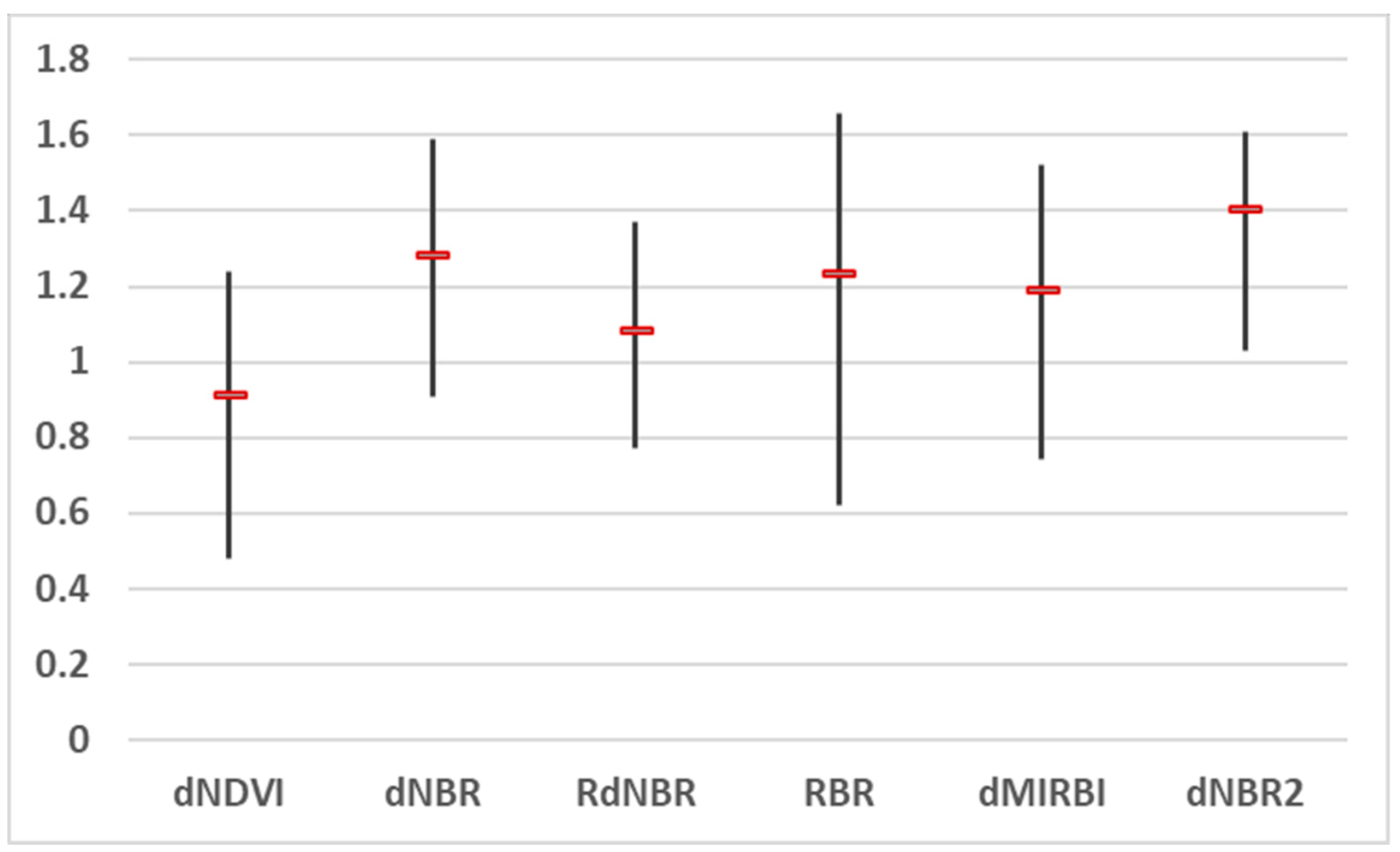
2.3. Selection of Fire Spectral Indices for the Buffer-From-Cluster Approach

The three spectral indices chosen to test the BFCA for the BA mapping application have been selected by accounting for the results of the analysis of the separability parameter [36], similarly to what was done in [37,38]. The separability between two thematic classes (burned/changed pixels and unburned/unchanged pixels in this case) is defined as:

$$S=\frac{\left|{\mu }_1-{\mu }_2\right|}{{\sigma }_1+{\sigma }_2}$$

(3)

where ${\mu }_1$ and ${\mu }_2$ are the mean values of the samples belonging to the classes and ${\sigma }_1$ and ${\sigma }_2$ are the corresponding standard deviations. By comparing Equations (2) and (3), it can be noted that the definition of S is quite similar to that of the Ashman’s coefficient. The separability between two classes is generally considered good if S > 1 and the higher S, the higher the separability [36,37,38].

S has been evaluated for the differences between the pre-fire and post-fire values of the following indices: Normalized Difference Vegetation Index (NDVI) [39] and Normalized Burn Ratio (NBR) [40] used in [22,41], and Normalized Burned Ratio 2 (NBR2) [42] and Mid-Infrared Burned Index (MIRBI) [43], used in [23,38]. These indices are defined as:

$$NDVI=\frac{{\rho }_{NIR}-{\rho }_{RED}}{{\rho }_{NIR}+{\rho }_{RED}}$$

(4)

$$NBR=\frac{{\rho }_{NIR}-{\rho }_{SWIR\_L}}{{\rho }_{NIR}+{\rho }_{SWIR\_L}}$$

(5)

$$NBR2=\frac{{\rho }_{SWIR\_S}-{\rho }_{SWIR\_L}}{{\rho }_{SWIR\_S}+{\rho }_{SWIR\_L}}$$

(6)

$$MIRBI=10·{\rho }_{SWIR\_L}-9.8·{\rho }_{SWIR\_S}+2$$

(7)

where NIR indicates the near infrared band, RED indicates the red band, and SWIR_L and SWIR_S are the short wave infrared long reflectance and short wave infrared short reflectance, respectively. The differences between the pre-fire and post-fire values of the aforementioned indices will be indicated hereafter as dNDVI, dNBR2, dNBR, and dMIRBI.

Besides dNBR, even its relativized forms proposed in the literature, namely the relativized dNBR (RdNBR) [44] and the relativized burn ratio (RBR) [45] have been considered in the separability analysis. These variables are defined as:

$$RdNBR=\frac{1000·dNBR}{\sqrt{\left|NB{R}_{pre-fire}\right|}}=\frac{1000·\left(NB{R}_{pre-fire}-NB{R}_{post-fire}\right)}{\sqrt{\left|NB{R}_{pre-fire}\right|}}$$

(8)

$$RBR=\frac{1000·dNBR}{NB{R}_{pre-fire}+1.001}$$

(9)

To perform the separability analysis, the S2 data listed in Table 2 have been used. For each case study, the BA class has been derived by gathering the pixels labelled as burned by CEMS. The class of unburned pixels has been generated by considering both a buffer zone around the BAs and by randomly collecting pixels in areas labelled as unburned by CEMS. When building up the class of unburned pixels, attention has been paid to include in each class at least 30% of the total sample pixels and to exclude clouds, snow and water bodies. The result of the analysis is shown in Figure 2.

Looking at Figure 2, it can be noted that the MTSIs that present the highest S between the classes of burned and unburned pixels are dNBR2 and dNBR. These MTSIs provide different information about a target, because NBR2 accounts for the SWIR bands while NBR considers SWIR_L and NIR bands. Conversely, RdNBR and RBR basically provide the same information as dNBR. Even dMIRBI presents a quite high value of S. Although MIRBI accounts for the SWIR bands like NBR2, it has been demonstrated in [38] that the distributions of burned and unburned classes are different for dNBR2 and dMIRBI. Hence, dNBR2, dNBR and dMIRBI have been selected as the MTSIs used to generate the maps of BA through the BFCA.

2.4. Application of the Buffer-From-Cluster Approach to Burned Area Mapping

The operations described in this section have been carried out for each test case. They have been implemented using the IDL programing language, and the ENVI routines that can be launched by means of specific IDL instructions. Firstly, the ISODATA clustering has been applied to the maps of dNBR2, dNBR and dMIRBI (excluding masked pixels). For burned pixels, the post-fire values of NBR and NBR2 tend to decrease with respect to the pre-fire ones [37,38,44,46], while the opposite occurs for MIRBI [23,38]. Hence, the clusters presenting the highest median value of dNBR and dNBR2 and the lowest median value of dMIRBI have been selected and then intersected, generating the clustering-derived changed (burned) area. Moreover, pixels presenting a negative value of dNBR or dNBR2, or a positive value of dMIRBI have been excluded from the clustering-derived changed area. To further increase the reliability of the clustering-derived changed area, even pixels whose NBR2_post-fire values were greater than the tile mean value of NBR2_post-fire or whose MIRBI_post-fire values were less than the tile mean value of MIRBI_post-fire have been removed as suggested in [38].

Successively, for each MTSI, the bimodality check has been performed. It has been marked as passed if it has been passed for at least two out of three MTSIs. It has been verified that this happened for all the test cases listed in Table 2 and that, for most of the test cases, bimodal histograms were obtained for all the MTSIs. For bimodal histograms, the Otsu’s method has been applied to determine the threshold Th, as described in Section 2.1.3. For the remaining non-bimodal histograms, the empirical thresholds proposed by in [38] for dNBR2 (0.05) and dMIRBI (−0.25) and in [46] for dNBR (260) have been used.

After having applied the RGA, the thresholding-derived BA has been combined with the clustering-derived one as described in Section 2.1.4 to produce, for each test case, a map of BAs. All the burned pixels grouped in patches of ground smaller than 10,000 m² (25 pixels) have not been labelled as burned, thus assuming 1 ha as minimum mapping unit for BA mapping from S2.

2.5. Water Index and Application of the Buffer-From-Cluster Approach to Flood Mapping

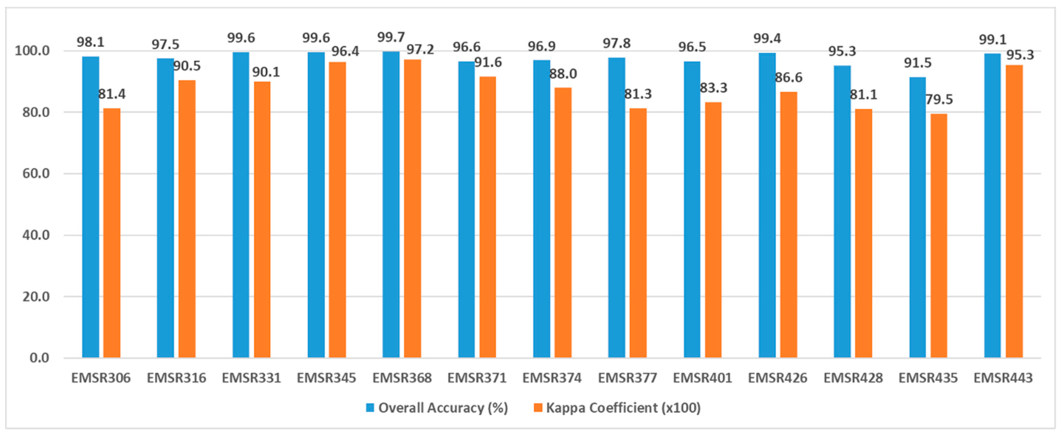
Two water indices are commonly used to map floodwater using multispectral data. They are the Normalized Difference Water Index (NDWI) [47] and the Modified Normalized Difference Water Index (MNDWI) [48]. Positive values of NDWI and MNDWI correspond to the presence of water. In this case, we have decided to test the BFCA using only one MTSI. The MNDWI has been selected and increases of MNDWI are searched for by BFCA to map flooded areas. Hence, in this case dMNDWI is computed as the difference between post-flood and pre-flood values of the MNDWI. The latter is defined as:

$$MNDWI=\frac{{\rho }_{GREEN}-{\rho }_{SWIR\_S}}{{\rho }_{GREEN}+{\rho }_{SWIR\_S}}$$

(10)

After having applied the ISODATA clustering, the clusters presenting the highest median value of dMNDWI have been selected to represent the clustering-derived changed (flooded) area. Pixels presenting a negative value of dMNDWI have been excluded from the clustering-derived changed area. The flood maps have been generated by combining the clustering-derived changed area with the thresholding-derived one.

2.6. Validation

To quantitatively represent the results of the comparison between BFCA-derived and CEMS-derived maps, a confusion matrix has been computed for each case study, assuming the CEMS-derived maps as ground truth. A confusion matrix summarizes the performance of a classification algorithm. From the confusion matrices, four accuracy metrics have been derived: overall accuracy (OA), kappa coefficient (κ), errors of commission (ε_comm), and omission (ε_om) for the class of changed areas. It must be considered that, if the extension of the changed area is small, the class of changed pixels is underrepresented compared to the other class (unchanged pixels). This implies that very high values of OA are often obtained. To tackle this problem, limited geographic areas have been considered to derive the confusion matrices. The boundaries of the geographic areas have been determined using the “area of interest” shapefile included in the CEMS data (see [22] for more details).

3. Results

Figure 3 shows a full example of the results of the BFCA for the Calci test site (EMSR316, see Table 2). It includes the intermediate results of the various steps of the BFCA and the final BA map. Looking at Figure 3, it can be noted that, for each MTSI, the cluster presenting the highest median of the pixel values (red color in the left panels) has been labelled as the class of changed pixels. The upper central panel shows that with a buffer zone of buffering distance 50 pixels, the clustering-derived changed area contains less than 30% of the pixels of the population formed by the union of the buffer zone and the clustering-derived changed area itself. The same occurs with a buffering distance of 25 pixels. Conversely, with a buffer zone of buffering distance 12 pixels (blue color in the upper central panel of Figure 3) bimodal histograms have been obtained, as confirmed by Figure 4, where the histograms of the pixel values of the population generated by merging the buffer zone with the clustering-derived changed area are presented for dNBR2, dNBR, and dMIRBI. The Gaussian fitting functions are also shown. It can be seen that, in this case, the GMM is suitable to describe the distribution of the pixel values. The following threshold values have been obtained: 0.19 for dNBR2, 0.35 for dNBR and −0.38 for dMIRBI.

Looking at the upper right panel of Figure 3, it can be deduced that a very noisy map would have been obtained by using only the ISODATA clustering. Conversely, an underestimation of the BA would have resulted from the simple application of the thresholding and region growing techniques. This can be inferred by looking also at the lower central panel of Figure 3, which includes the boundary of the CEMS-derived BA too.

Figure 5 shows, for the EMSR342 test case, the histograms of the pixel values of dMNDWI for the clustering-derived changed area and the buffer zone (S2 tile T54KVE). The latter histogram has been generated with a final value of the buffering distance equal to 25 pixels. A threshold value equal to 0.59 has been obtained. Even in this case the GMM properly describes the distribution of the pixel values. Figure 6 presents the result of the mosaicking of the flood maps produced by applying the BFCA to the four tiles listed in Table 3.

The results of the comparison between BFCA-derived and CEMS-derived maps, expressed in terms of the accuracy metrics introduced in Section 2.6 are synthetically presented in Figure 7 (OA and κ) and Figure 8 (ε_comm and ε_om) for the BA mapping application.

The OA always exceeds 91% with an average value (over the 13 test cases considered here) of 97.5%, while κ is in the range [0.80–0.97] with an average value of 0.88. With respect to the errors, ε_comm ranges between 1.1% and 29.8% with an average value of 10.3%, while ε_om is in the range [0.2%–26.3%] with an average value equal to 9.5%. We have also calculated the errors for all the pixels in the 13 tiles together obtaining in this case ε_comm = 4.3% and ε_om = 11.3%.

As for the flood mapping application, the following values of the values of the accuracy metrics have been obtained: OA = 91.1%, κ = 0.80, ε_comm = 12.1%, ε_om = 0.5%.

4. Discussion

This paper presents a new method to automatically perform binary change detection in MTSIs conceived to map the extent of the area affected by a natural disaster like wildfire. Several approaches dealing with unsupervised binary change detection in MTSIs are available in the literature (see the Introduction for some references). Most of them are generally quite complex using complicated data modeling and parameter estimation. The proposed method represents a rapid approach that aims at joining computational efficiency and good accuracy.

4.1. Computational Efficiency and Accuracy

As for the computational efficiency, although, before carrying out the automatic thresholding, the BFCA uses ISODATA clustering, the latter is not significantly time consuming even if it is applied sequentially to three MTSIs, as done for the BA mapping application, mainly because just an iteration is used to cluster the pixels. Even the fitting of the histograms of changed and unchanged pixels with a Gaussian function is not time consuming (a maximum of 20 iteration has been fixed). It takes about 10 min to process a S2 image tile (5490 × 5490 pixels) using an i7-7800X 3.5GHz processor with 128 GB RAM.

As for the accuracy, looking at Figure 7 and Figure 8, it can be deduced that a fairly good agreement between CEMS-derived and BFCA-derived BA maps has been obtained for the case studies considered here. In the literature, using S2 data and fully automatic BA mapping algorithms, omission errors equal to around 40% [49] and 26.5% [38] and commission errors of 19.3% [38] and 25% have been obtained [49]. Hence, average values around 10% for both errors can be considered as an indication that the BFCA works well in the identification of BAs from S2 data.

The case studies listed in the first five rows of Table 1 (EMSR306-368) were also analyzed in [22], where a SBA was used in combination with clustering. A significant reduction of ε_om has been achieved through the BFCA, although this implied a slight increase of ε_comm. A significant improvement of the results has been obtained in particular for the EMSR331 case study. The agreement with the CEMS-derived BA maps has increased also for the EMSR345 and EMSR 368 test cases, while for the EMSR306 and EMSR316 test cases, the decrease of ε_om has been compensated by an increase of ε_comm. It must be pointed out that the improvement of the performances of the BA mapping is due not only to the use of the BFCA, but also to a more accurate choice of the MTSIs, performed through the analysis of the separability between classes. To support this hypothesis, the algorithm proposed in [22] has been applied to the MTSIs used for BA mapping. For some test cases, e.g., EMSR316, values of the accuracy metrics very similar to those obtained using the BFCA have been achieved. For other test cases, a worsening of the performances with respect to those achieved through the BFCA has been observed. For instance, for the EMSR435 test case, ε_om has increased from 23.1% (BFCA) to 24.2% and for the EMSR428 test case it has increased from 26.3% (BFCA) to 27.3%. The great importance of selecting suitable variables to detect changes in any change detection problem is pointed out in [3]. The case studies listed in Table 2 include fires having very different extents from about 1 km² (EMSR401 test case) to about 170 km². The use of a medium-high resolution instrument like S2 contributed to the quite low values of ε_om (e.g., 10.3% for the EMSR401 test case) achieved when fire burned few km² of surface. It can be expected that the BFCA might underestimate small-size fires using MTSIs derived from coarser resolution data. In [27,38,50], missed detection of fires having a size less than 1 km² has been ascribed to the use of data having a coarse spatial resolution (250–500 m).

The highest value of ε_comm (29.8%) has been obtained for the EMSR377 case study. However, in this case the CEMS-derived maps have been produced using the data from a different satellite (SPOT-6/7). This may have an impact on the agreement between the BA maps especially if a small area (3.4 km² for EMSR377, see Table 2) is affected by fire, because in this case the fire likely had a quite low intensity and an ambiguous spectral signature.

The highest value of ε_om (26.3%) has been obtained for the EMSR428 case study. Figure 9 shows an RGB color composite of the pre-fire (red) and post-fire (green and blue) dNBR2 data used to map the Tasarte fire (EMSR428). It can be noted that some areas classified as burned by CEMS appear in cyan tone; this indicates that NBR2 increased rather than decrease, as expected in a BA, thus explaining the large value of ε_om. Note that even a Pleaides post-fire image acquired on the same day as the S2 one has been analyzed by CEMS to produce the BA map. This could at least partially explain the discrepancy, considering that Pleiades do not have SWIR bands.

For what concerns flood mapping, it has been chosen to test the performances of the BFCA using just one MTSI, obtaining again a good agreement with reference data. The high OA (91.1%) is significant for the EMSR342 case study, because in this case the class of changed/flooded pixels is not underrepresented with respect to the other one. Using S2-derived dMNDWI data at a resolution of 20 m, commission errors ranging from 2% to 7.6% (lower than the ε_comm value obtained through the BFCA for the EMSR342 case study) and omission errors in the range [9–42.1%] (considerably higher than the ε_om value obtained through the BFCA for the EMSR342 case study) have been reported in [51], but analyzing a very different study area (the Venice coastland) and only very small portions of the images (2 × 2 km²). Even in this case, it is expected that combining more MTSIs could lead to the achievement of better accuracies, as discussed in [52], where quite high omission and commission errors (generally higher than those obtained through the BFCA for the EMSR342 case study) were reported by applying crisp thresholds to single MTSIs.

It must be pointed out that, while the effect of a wildfire can be assessed even several days after the event (e.g., reforestation generally takes a long time), the temporal scale of flood events can be very fast. For instance, the possibility to map flash floods vanishes few hours after the occurrence of the event. Even if flood mapping using multispectral instruments like S2 can provide good performances, microwave instruments, capable to operate in almost all-weather conditions and during both day-time and night-time, are generally more suitable to map floods also because of the sensitivity of the microwave radiation to water [53]. Hence, flood mapping is more commonly carried out using synthetic aperture radar (SAR) (e.g., [54,55]), which joins the aforementioned characteristics of microwave sensors to a high spatial resolution (that ranges from hundreds of meters to less than 1 m).

4.2. Combination of Different Image Processing Techniques

The combination of different image processing techniques is not new for what concerns BA mapping (e.g., [56]), flood mapping (e.g., [25,34]), and change detection in general (e.g., [7], where clustering was used in combination with principal components analysis). Here, clustering is basically used to estimate two distribution functions, one representing the class of changed pixels and the other one representing the background. Nonetheless, it has also a role in determining the final classification because objects belonging to the clustering-derived changed area are finally classified as changed if they include seeds of the RGA (see Section 2.1.4). Although, for BA mapping, the clustering-derived changed area is generated by the sequential application of the ISODATA to different MTSIs, the intra-class variability in each MTSI can be high, so that ISODATA may not produce a very accurate classification. Looking at the upper right panel of Figure 3, it can be seen that ISODATA is generally able to identify the BA, but many false alarms may be raised. On the other hand, the application of the thresholding, even if performed in the framework of an RGA, is very sensitive to uncertainties in the determination of the seeds and the tolerances of the RGA. Since the BFCA fits the distributions of changed and unchanged pixels by assuming a GMM, an imperfect fitting can imply imperfect estimations of the thresholds and the tolerances.

To further underline the importance of combining different techniques, BA maps have also been produced by using a thresholding algorithm with thresholds derived from the SBA and applied within the framework of an RGA. The individual maps derived from the application of SBA, thresholding and RGA to each MTSI have been combined through a logical AND (i.e., intersected) and through a logical OR (i.e., merged). For the first case (map intersection) an increase of the omission error has been generally observed. For instance, for the EMSR316 test case, ε_om has increased from 3.1% (BFCA) to 25.4% and for the EMSR428 test case it has exceeded 50%. As expected, for map merging, the opposite occurs. For instance, for the EMSR316 test case, ε_comm has increased from 15.2% (BFCA) to 24.3%.

The values of the accuracy metrics shown in Figure 7 and Figure 8 suggest that the combination of clustering and thresholding succeeds in compensating the errors related to the application of each technique alone.

4.3. Maximum Number of Clusters and Initail Buffering Distance

Figure 10 shows, for one MTSI (dNBR2), the ISODATA outputs obtained by selecting different values for the maximum number of classes: 5, 10, and 15. The EMSR316 test case has been used to carry out the exercise (hence the central panel of Figure 10 is the same as the upper left panel of Figure 3). The pixels belonging to the class having the highest median of the dNBR2 pixel values (red color in Figure 10) are almost the same in the three maps. For the BFCA, it is fundamental that the majority of changed pixels are identified by the ISODATA because it is basically used to estimate the distribution of this population. Hence, if among the classes of unchanged pixels discriminated by the ISODATA, which can for instance represent different types of land cover, oversegmentation or undersegmentation occur, this does not represent a problem for the accuracy of the BFCA.

Besides the selection of the maximum number of classes, another arbitrary choice done to implement the BFCA is the initial value of the buffering distance (50 pixels). Looking at the upper central panel of Figure 3, it can be noted that the initial buffer zone (grey color) covers a large part of the spatial subset around the area affected by the fire shown in the figure. This is due to the quite large number of small objects belonging to the class of changed pixels. In principle, for each object belonging to the class of changed pixels, a different dimension of the buffering distance, proportional to the size of the object, should be used. However, this would imply a significant decrease of the computational efficiency, especially if many objects belong to the class of interest. In the BFCA the buffer is mainly used to derive a bimodal histogram for the population formed by the selected changed and unchanged pixels. The adaptive modification of the buffering distance is an efficient way to mitigate this problem. Its increase/decrease ensures that two distinguishable modes are present in the histograms as confirmed by Figure 4 (and Figure 5 for flood mapping). Hence, it is not worthwhile to decrease the computational efficiency of the BFCA if this goal is achieved without generating different buffer sizes for objects of different sizes.

In [27], unburned pixels around burned ones are searched for within a strip whose length has been empirically set between 10 and 20 km in order to determine a suitable threshold to identify BA. This strip is placed around a buffer having a distance of 1875 m. In [27], no adaptive modification of the strip and the buffer size is performed. It is worth noting that, for a pixel size of 20m, a buffering distance of 50 pixels corresponds to 1 km. Using 250-m resolution data, like the MODIS highest resolution ones from which BA maps are produced in [27], a range between 10 and 20 km corresponds to a buffering distance of 40–80 pixels. Hence, using the BFCA for coarse spatial resolution data (250–500 m), an initial buffering distance greater than that chosen for S2 (e.g., 80 pixels) can be used.

5. Conclusions and Perspectives

The new Buffer-From-Cluster Approach (BFCA) to automatically perform binary change detection in multitemporal spectral indices has been presented. It has been conceived to map the extent of areas affected by a natural hazard like wildfire. The BFCA combines different image processing techniques such as clustering and thresholding, which are applied within the framework of a region growing algorithm. Nonetheless, it is quite simple in terms of computation and effective in identifying changes caused by the occurrence of a disaster. It is therefore suitable for real-time applications, especially if a large amount of multispectral data has to be processed, for instance for routinely producing maps of areas affected by disasters.

The effectivity of the BFCA in the identification of changes caused by the occurrence of a disaster has been verified by comparing BFCA-derived burned area maps, generated using Sentinel-2 data, with maps produced by the CEMS. Values around 10% for omission and commission errors have been obtained considering the average over all the case studies. They never exceeded 30%, while the overall accuracy always exceeded 91%.

The values of the accuracy metrics seem to indicate that the BFCA provides results better than those found in the literature for automatic burned areas mapping using Sentinel-2 data and fully automatic algorithms. However, more tests are necessary to confirm this indication. For this purpose, it is planned to make available the BA mapping algorithm derived from the BFCA in the WASDI platform (www.wasdi.net), where registered users will be able to test it on their own Sentinel-2 data. In addition, starting from summer 2020, this algorithm will update a previous version implemented to provide, for the Italian territory, a daily service of burned areas mapping based on Sentinel-2 data [22].

Although burned areas mapping has been chosen as the main application of the BFCA, the latter has been conceived to be applied also to other disasters like floods. A test for this kind of application gave encouraging results (omission error of 0.5%, commission error of 12%). Even the algorithm for flood mapping using Sentinel-2 data based on the BFCA will be made available through the WASDI platform. However, it must be pointed out that the inability of multispectral instruments to provide data when cloud cover is present or during night-time strongly limits their effectivity for flood mapping. Therefore, future work will evaluate the possibility to adapt the BFCA to flood mapping from SAR, which is the most suitable sensor for this application.

References

1. Dilley, M.; Chen, R.S.; Deichmann, U.; Lerner-Lam, A.; Arnold, M.; Agwe, J.; Buys, P.; Kjekstad, O.; Lyon, B.; Yetman, G. Natural Disaster Hotspots: A Global Risk Analysis; World Bank Publications: Washington, DC, USA, 2005. [Google Scholar]
2. Petiteville, I.; Ward, S.; Dyke, G.; Steventon, M.; Harry, J. Satellite Earth Observations in Support of Disaster Risk Reduction; Special 2015 WCDRR Edition; ESA Publication: Auckland, New Zealand, 2015. [Google Scholar]
3. Lu, D.; Li, G.; Moran, E. Current situation and needs of change detection techniques. Int. J. Image Data Fusion 2014, 5, 13–38. [Google Scholar] [CrossRef]
4. Bovolo, F.; Bruzzone, L. A Split-Based Approach to Unsupervised Change Detection in Large-Size Multitemporal Images: Application to Tsunami-Damage Assessment. IEEE Trans. Geosci. Remote Sens. 2007, 45, 1658–1669. [Google Scholar] [CrossRef]
5. Bruzzone, L.; Prieto, D.F. Automatic analysis of the difference image for unsupervised change detection. IEEE Trans. Geosci. Remote Sens. 2000, 38, 1171–1182. [Google Scholar] [CrossRef] [Green Version]
6. Li, H. Accurate and efficient classification based on common principal components analysis for multivariate time series. Neurocomputing 2016, 171, 744–753. [Google Scholar] [CrossRef]
7. Celik, T. Unsupervised change detection in satellite images using principal component analysis and κ-means clustering. IEEE Geosci. Remote Sens. Lett. 2009, 6, 772–776. [Google Scholar] [CrossRef]
8. Chen, J.; Gong, P.; He, C.; Pu, R.; Shi, P. Land-use/land-cover change detection using improved change-vector analysis. Photogramm. Eng. Remote Sens. 2003, 69, 369–379. [Google Scholar] [CrossRef] [Green Version]
9. Bovolo, F.; Bruzzone, L. A theoretical framework for unsupervised change detection based on change vector analysis in the polar domain. IEEE Trans. Geosci. Remote Sens. 2007, 45, 218–236. [Google Scholar] [CrossRef] [Green Version]
10. Nordberg, M.L.; Evertson, J. Vegetation index differencing and linear regression for change detection in a Swedish mountain range using Landsat TM® and ETM+® imagery. L. Degrad. Dev. 2005, 16, 139–149. [Google Scholar] [CrossRef]
11. Tewkesbury, A.P.; Comber, A.J.; Tate, N.J.; Lamb, A.; Fisher, P.F. A critical synthesis of remotely sensed optical image change detection techniques. Remote Sens. Environ. 2015, 160, 1–14. [Google Scholar] [CrossRef] [Green Version]
12. Ban, Y.; Yousif, O. Change Detection Techniques: A Review. In Multitemporal Remote Sensing: Methods and Applications; Ban, Y., Ed.; Springer International Publishing: Cham, Switzerland, 2016; pp. 19–43. ISBN 978-3-319-47037-5. [Google Scholar]
13. Kittler, J.; Illingworth, J. Minimum error thresholding. Pattern Recognit. 1986, 19, 41–47. [Google Scholar] [CrossRef]
14. Otsu, N. A Threshold Selection Method from Gray Level Histograms. IEEE Trans. Syst. Man. Cybern. 1979, 9, 62–66. [Google Scholar] [CrossRef] [Green Version]
15. Rogerson, P.A. Change detection thresholds for remotely sensed images. J. Geogr. Syst. 2002, 4, 85–97. [Google Scholar] [CrossRef]
16. Glasbey, C.A. An Analysis of Histogram-Based Thresholding Algorithms. Graph. Models Image Process. 1993, 55, 532–537. [Google Scholar] [CrossRef]
17. Zhan, Y.; Zhang, G. An improved OTSU algorithm using histogram accumulation moment for ore segmentation. Symmetry 2019, 11, 431. [Google Scholar] [CrossRef] [Green Version]
18. Kapur, J.N.; Sahoo, P.K.; Wong, A.K.C. A new method for gray-level picture thresholding using the entropy of the histogram. Comput. Vis. Graph. Image Process. 1985, 29, 273–285. [Google Scholar] [CrossRef]
19. Chini, M.; Hostache, R.; Giustarini, L.; Matgen, P. A hierarchical split-based approach for parametric thresholding of SAR images: Flood inundation as a test case. IEEE Trans. Geosci. Remote Sens. 2017, 55, 6975–6988. [Google Scholar] [CrossRef]
20. Haralick, R.M.; Shapiro, L.G. Survey: Image Segmentation Techniques. Comput. Vis. Graph. Image Process. 1985, 29, 100–132. [Google Scholar] [CrossRef]
21. Adams, R.; Bischof, L. Seeded Region Growing. IEEE Trans. Pattern Anal. Mach. Intell. 1994, 16, 641–647. [Google Scholar] [CrossRef] [Green Version]
22. Pulvirenti, L.; Squicciarino, G.; Fiori, E.; Fiorucci, P.; Ferraris, L.; Negro, D.; Gollini, A.; Severino, M.; Puca, S. An automatic processing chain for near real-time mapping of burned forest areas using sentinel-2 data. Remote Sens. 2020, 12, 674. [Google Scholar] [CrossRef] [Green Version]
23. Stroppiana, D.; Bordogna, G.; Carrara, P.; Boschetti, M.; Boschetti, L.; Brivio, P.A. A method for extracting burned areas from Landsat TM/ETM+ images by soft aggregation of multiple Spectral Indices and a region growing algorithm. ISPRS J. Photogramm. Remote Sens. 2012, 69, 88–102. [Google Scholar] [CrossRef]
24. Plank, S.; Martinis, S. A fully automatic burnt area mapping processor based on AVHRR Imagery-A TIMELINE thematic processor. Remote Sens. 2018, 10, 341. [Google Scholar] [CrossRef] [Green Version]
25. Matgen, P.; Hostache, R.; Schumann, G.; Pfister, L.; Hoffmann, L.; Savenije, H.H.G. Towards an automated SAR-based flood monitoring system: Lessons learned from two case studies. Phys. Chem. Earth 2011, 36, 241–252. [Google Scholar] [CrossRef]
26. Stroppiana, D.; Boschetti, M.; Azar, R.; Barbieri, M.; Collivignarelli, F.; Gatti, L.; Fontanelli, G.; Busetto, L.; Holecz, F. In-season early mapping of rice area and flooding dynamics from optical and SAR satellite data. Eur. J. Remote Sens. 2019, 52, 206–220. [Google Scholar] [CrossRef] [Green Version]
27. Lizundia-Loiola, J.; Otón, G.; Ramo, R.; Chuvieco, E. A spatio-temporal active-fire clustering approach for global burned area mapping at 250 m from MODIS data. Remote Sens. Environ. 2020, 236, 111493. [Google Scholar] [CrossRef]
28. Smiraglia, D.; Filipponi, F.; Mandrone, S.; Tornato, A.; Taramelli, A. Agreement index for burned area mapping: Integration of multiple spectral indices using Sentinel-2 satellite images. Remote Sens. 2020, 12, 1862. [Google Scholar] [CrossRef]
29. Richards, J.A.; Jia, X. Remote Sensing Digital Image Analysis: An Introduction; Springer: Berlin/Heidelberg, Germany, 2006; ISBN 3540251286. [Google Scholar]
30. Vilasa, L.; Miralles, D.G.; De Jeu, R.A.M.; Dolman, A.J. Global soil moisture bimodality in satellite observations and climate models. J. Geophys. Res. Atmos. 2017, 122, 4299–4311. [Google Scholar] [CrossRef] [Green Version]
31. Guide, S.A.S.U. SAS/STAT User’s Guide, version 6; SAS Institute Inc.: Cary, NC, USA, 1990. [Google Scholar]
32. Pfister, R.; Schwarz, K.A.; Janczyk, M.; Dale, R.; Freeman, J.B. Good things peak in pairs: A note on the bimodality coefficient. Front. Psychol. 2013, 4, 700. [Google Scholar] [CrossRef] [Green Version]
33. Ashman, K.A.; Bird, C.M.; Zepf, S.E. Detecting bimodality in astronomical datasets. Astron. J. 1994, 108, 2348–2361. [Google Scholar] [CrossRef]
34. Boni, G.; Ferraris, L.; Pulvirenti, L.; Squicciarino, G.; Pierdicca, N.; Candela, L.; Pisani, A.R.; Zoffoli, S.; Onori, R.; Proietti, C.; et al. A Prototype System for Flood Monitoring Based on Flood Forecast Combined with COSMO-SkyMed and Sentinel-1 Data. IEEE J. Sel. Top. Appl. Earth Obs. Remote Sens. 2016, 9, 2794–2805. [Google Scholar] [CrossRef]
35. European Environment Agency, Corine Land Cover. 2018. Available online: https://land.copernicus.eu/pan-european/corine-land-cover/clc2018 (accessed on 14 August 2020).
36. Kaufman, Y.J.; Remer, L.A. Detection of Forests Using Mid-IR Reflectance: An Application for Aerosol Studies. IEEE Trans. Geosci. Remote Sens. 1994, 32, 672–683. [Google Scholar] [CrossRef]
37. Lasaponara, R. Estimating spectral separability of satellite derived parameters for burned areas mapping in the Calabria region by using SPOT-Vegetation data. Ecol. Modell. 2006, 196, 265–270. [Google Scholar] [CrossRef]
38. Roteta, E.; Bastarrika, A.; Padilla, M.; Storm, T.; Chuvieco, E. Development of a Sentinel-2 burned area algorithm: Generation of a small fire database for sub-Saharan Africa. Remote Sens. Environ. 2019, 222, 1–17. [Google Scholar] [CrossRef]
39. Tucker, C.J. Red and Photographic Infrared Linear Combinations for Monitoring Vegetation. Remote Sens. Environ. 1979, 8, 127–150. [Google Scholar] [CrossRef] [Green Version]
40. Key, C.H.; Benson, N. The Normalized Burn Ratio (NBR): A Landsat TM Radiometric Measure of Burn Severity; Northern Rocky Mountain Science Center: Bozeman, MT, USA, 1999.
41. Navarro, G.; Caballero, I.; Silva, G.; Parra, P.C.; Vázquez, Á.; Caldeira, R. Evaluation of forest fire on Madeira Island using Sentinel-2A MSI imagery. Int. J. Appl. Earth Obs. Geoinf. 2017, 58, 97–106. [Google Scholar] [CrossRef] [Green Version]
42. García, M.J.L.; Caselles, V. Mapping burns and natural reforestation using thematic mapper data. Geocarto Int. 1991, 6, 31–37. [Google Scholar] [CrossRef]
43. Trigg, S.; Flasse, S. An evaluation of different bi-spectral spaces for discriminating burned shrub-savannah. Int. J. Remote Sens. 2001, 22, 2641–2647. [Google Scholar] [CrossRef]
44. Miller, J.D.; Thode, A.E. Quantifying burn severity in a heterogeneous landscape with a relative version of the delta Normalized Burn Ratio (dNBR). Remote Sens. Environ. 2007, 109, 66–80. [Google Scholar] [CrossRef]
45. Parks, S.A.; Dillon, G.K.; Miller, C. A new metric for quantifying burn severity: The relativized burn ratio. Remote Sens. 2014, 6, 1827–1844. [Google Scholar] [CrossRef] [Green Version]
46. Botella-Martínez, M.A.; Fernández-Manso, A. Estudio de la severidad post-incendio en la comunidad Valenciana comparando los índices dNBR, RdNBR y RBR a partir de imágenes landsat 8. Rev. Teledetec. 2017, 2017, 33–47. [Google Scholar] [CrossRef] [Green Version]
47. McFeeters, S.K. The use of the Normalized Difference Water Index (NDWI) in the delineation of open water features. Int. J. Remote Sens. 1996, 17, 1425–1432. [Google Scholar] [CrossRef]
48. Xu, H. Modification of normalised difference water index (NDWI) to enhance open water features in remotely sensed imagery. Int. J. Remote Sens. 2006, 27, 3025–3033. [Google Scholar] [CrossRef]
49. Filipponi, F. Exploitation of Sentinel-2 Time Series to Map Burned Areas at the National Level: A Case Study on the 2017 Italy Wildfires. Remote Sens. 2019, 11, 622. [Google Scholar] [CrossRef] [Green Version]
50. Chuvieco, E.; Mouillot, F.; van der Werf, G.R.; San Miguel, J.; Tanasse, M.; Koutsias, N.; García, M.; Yebra, M.; Padilla, M.; Gitas, I.; et al. Historical background and current developments for mapping burned area from satellite Earth observation. Remote Sens. Environ. 2019, 225, 45–64. [Google Scholar] [CrossRef]
51. Du, Y.; Zhang, Y.; Ling, F.; Wang, Q.; Li, W.; Li, X. Water bodies’ mapping from Sentinel-2 imagery with Modified Normalized Difference Water Index at 10-m spatial resolution produced by sharpening the swir band. Remote Sens. 2016, 8, 354. [Google Scholar] [CrossRef] [Green Version]
52. Goffi, A.; Stroppiana, D.; Brivio, P.A.; Bordogna, G.; Boschetti, M. Towards an automated approach to map flooded areas from Sentinel-2 MSI data and soft integration of water spectral features. Int. J. Appl. Earth Obs. Geoinf. 2020, 84, 101951. [Google Scholar] [CrossRef]
53. Pierdicca, N.; Pulvirenti, L.; Chini, M.; Guerriero, L.; Candela, L. Observing floods from space: Experience gained from COSMO-SkyMed observations. Acta Astronaut. 2013, 84, 122–123. [Google Scholar] [CrossRef]
54. Chini, M.; Pelich, R.; Pulvirenti, L.; Pierdicca, N.; Hostache, R.; Matgen, P. Sentinel-1 InSAR Coherence to Detect Floodwater in Urban Areas: Houston and Hurricane Harvey as A Test Case. Remote Sens. 2019, 11, 107. [Google Scholar] [CrossRef] [Green Version]
55. Pulvirenti, L.; Chini, M.; Pierdicca, N.; Boni, G. Use of SAR data for detecting floodwater in urban and agricultural areas: The role of the interferometric coherence. IEEE Trans. Geosci. Remote Sens. 2016, 54, 1532–1544. [Google Scholar] [CrossRef]
56. Bastarrika, A.; Chuvieco, E.; Martín, M.P. Mapping burned areas from landsat TM/ETM+ data with a two-phase algorithm: Balancing omission and commission errors. Remote Sens. Environ. 2011, 115, 1003–1012. [Google Scholar] [CrossRef]
Figure 1. Flowchart of the Buffer-From-Cluster Approach. Rectangles denote operations; parallelograms denote data.
Remotesensing 12 02681 g001
Figure 2. Mean value (red horizontal lines) plus/minus standard deviation of the separability for the multitemporal spectral indices considered in this study.
Remotesensing 12 02681 g002
Figure 3. Full example of the results of the BFCA for the EMSR316 test case. Upper left panel (a): output of the ISODATA applied to dNBR2. Central left panel (b): output of the ISODATA applied to dNBR. Lower left panel (c): output of the ISODATA applied to dMIRBI. Upper central panel (d): clustering-derived changed area and buffer zone. Lower central panel (e): thresholding-derived changed area. Upper right panel (f): pixels belonging to both clustering-derived and thresholding-derived BAs (orange), only to the clustering-derived BA (purple), only to the thresholding-derived BA (green). Lower right panel (g): final BA map. All the maps are zoomed on the area affected by the fire. The magenta lines in panel (e) represent the boundary of the CEMS-derived burned area.
Remotesensing 12 02681 g003
Figure 4. Histograms (continuous lines) of the pixel values of dNBR2 (a), dNBR (b) and dMIRBI multiplied by −1 (c), for the clustering-derived changed areas (red) and the buffer zones (blue) shown in the upper central panel of Figure 3 (EMSR316 case study). The dashed lines represent the Gaussian fitting functions.
Remotesensing 12 02681 g004
Figure 5. Histograms (continuous lines) of the pixels values of dMNDWI for the clustering-derived changed area (red) and the buffer zone (blue). The EMSR342 test case (Queensland flood) and the T54KVE tile are considered. The dashed lines represent the Gaussian fitting functions.
Remotesensing 12 02681 g005
Figure 6. BFCA-derived flooded area map for the EMSR342 test case (Queensland flood). Cyan: flooded; blue: permanent water; grey: masked (cloudy) pixels; white: non-flooded; black: unclassified.
Remotesensing 12 02681 g006
Figure 7. Agreement between CEMS-derived and BFCA-derived BA maps represented in terms of overall accuracy and kappa coefficient (multiplied by 100).
Remotesensing 12 02681 g007
Figure 8. Disagreement between CEMS-derived and BFCA-derived BA maps represented in terms of omission and commission errors for the class of burned pixels.
Remotesensing 12 02681 g008
Figure 9. RGB color composite of the S2 images of the Tasarte fire (EMSR428). Red: NBR2pre-fire; green and blue: NBR2post-fire. The magenta line represents the boundary of the CEMS-derived burned area.
Remotesensing 12 02681 g009
Figure 10. Output of the ISODATA applied to dNBR2 obtained by assuming 5 (a), 10 (b) and 15 (c) as the maximum number of clusters. The EMSR316 test case is considered.
Remotesensing 12 02681 g010