1. Introduction
Recent Earth observation systems provide optical imagery at high spatial, spectral, and temporal resolutions, that allow for land cover maps containing agricultural, natural, and artificial classes to be produced over wide regions. While using a pixel-based approach provides accurate results on many land cover classes, especially on different crops [
1,
2,
3,
4], certain land cover types remain challenging to identify precisely, even with rich multi-spectral and multi-temporal information [
5].
With the high spatial resolution necessary to provide a precise outline and localization of the various land cover elements comes an significant issue: in general, each individual pixel covers a very limited area of the object that contains it. For example, in land cover mapping, artificial classes such as roads, urban cover, and industrial areas are made up of asphalted surfaces, vegetation, and buildings. This implies that the information contained in each pixel alone, the set of so-called pixel features, can be insufficient to fully characterize the target class. In fact, the spatial arrangement and proportion of the basic land cover elements can be a discriminating factor for telling apart such context-dependent classes.
For supervised classification methods to tackle this issue, information from beyond the pixel must be included in some way. The group of pixels, often adjacent in the image, that all participate in the decision regarding the target pixel are defined as the spatial support. Supervised methods that are currently employed to perform this task can be divided principally into two groups: model-based approaches and contextual feature approaches, which differ in their way of interpreting the spatial support.
The first group of methods, called model-based approaches here, involves providing the entirety of the spatial support of the target pixel as an input to the classification model. However, the number of pixels contained in a spatial support increases in a quadratic manner with its size. In order to deal with a large number of features in an efficient way, the supervised classification model must be tailored to the task at hand.
Today, a very popular model-based approach to tackle the issue of context-dependent classes is to use a Convolutional Neural Network (CNN) [
6], which is a supervised classification method that aims to learn both the feature extraction and the decision steps in an end-to-end manner, from the training data that have been provided. By using techniques like data augmentation, dropout regularization [
7], and batch normalization, these neural networks may achieve very strong performances on image classification problems, when sufficient quantities of labeled data are available [
8,
9,
10,
11]. CNNs have more recently been extended to the problem of labeling each pixel in an image, rather than labeling each patch individually. This problem is known as semantic segmentation in computer vision, but has sometimes been referred to as classification by the Remote Sensing community. In this paper, the term dense classification is used, to avoid ambiguity.
Many studies show that the recognition rate of context-dependent classes is improved by the use of CNNs, when compared to pixel-based classification. However, a deeper analysis suggests that such methods have difficulty providing geometrically precise results, as will be illustrated further in
Section 3. Recent attempts have been made to include geometric information into the CNN training process to counteract undesirable effects like the smoothing of sharp corners and the removal of small elements. For instance, in [
12], the authors combine a regular CNN with an edge detecting CNN, the Holistically-Nested Edge Detection network [
13], in order to improve the classification performance in these sensitive areas. However, the authors of these studies do not address the case where no dense reference data are available for training.
Generally speaking, CNNs are challenging to use for land cover map production, especially over large territories, as the reference data used for training are only available in a sparse form, in other words, not every pixel of the training patches is labeled. This is very often the case in land cover mapping, as the reference data come from a combination of existing geodatabases [
5], which each contain specific classes from the desired nomenclature. This means that the fine details of the geometry, the class edges, and the spatial relations between various classes are not directly present in the training data. This might make training difficult, as the CNN attempts to learn the feature extraction step from the data itself. Moreover, most of the past studies that apply CNN models to land cover mapping compare this approach to pixel-based classifications and, therefore, it is impossible to know whether the improvements come from the feature extraction, or from the fact that CNN models inherently take into account spatial context.
For these reasons, methods that were state-of-the-art before the arrival of Deep Learning are reconsidered here. Rather than using an end-to-end optimization, there exist several approaches based on the manual selection of contextual features, which describe a group of adjacent pixels known as the spatial support of the feature. Contextual features often seek to convey notions such as homogeneity or texture, or the presence of certain geometrical features like sharp angles, local extrema, or particular spatial frequencies. The selection of features is often relatively generic, but can also be guided by knowledge of the data and of the problem, as well as experience from similar cases. Using contextual features allows the prediction of the class label of the target pixel to be made according to a certain aspect of the behavior of the pixels in its neighborhood. Often, contextual features are combined with a general supervised classification method such as Support Vector Machine (SVM) [
14] or Random Forest (RF) [
15].
Practically speaking, using contextual features involves first defining a strategy for selecting a context around each pixel. If a square shape is taken everywhere, the method is known as a sliding window method. An example of a very common feature used in sliding windows is the Greyscale Level Co-occurence Matrix (GLCM), also known as the Haralick Texture [
16], which is based on a directional texture detection in a square neighborhood, and has previously been used in land cover mapping applications [
17,
18].
The other option is to consider an adaptive window around each pixel, which should respect the boundaries of the object containing the pixel. An object is defined as a connected area that represents an element of the nomenclature. Objects can be used as spatial supports for calculating contextual features. This is the basic idea behind Object Based Image Analysis (OBIA) [
19], where an image segmentation is applied to define different areas in the image, which are used instead of pixels as the base unit for classification. Often, low order statistics like the mean and variance are combined with contour descriptors, like the perimeter or compactness, to provide a contextual description of the segments [
20,
21]. Choosing a strategy for defining the neighborhood, and deciding which and how many contextual features to use is not simple, and relies on a degree of human expertise. However, one advantage is that these methods are usually faster than CNNs. Moreover, as their design is not based on an end-to-end optimization scheme, but on the inclusion of prior structure through the use of hand-crafted features in adaptive spatial supports, it is worth questioning whether these methods are more or less sensitive to incomplete training data.
A new methodology for including contextual information is presented in this study: the Histogram of Auto-Context Classes in Superpixels (HACCS), detailed in
Section 2, which makes up the principal contribution of this paper. The HACCS method involves integrating semantic cues in one or more adaptive spatial supports around the target pixel, by using an initial dense classification of the image.
Superpixel segmentation is based on the maximization of both feature homogeneity in the segments, and segment compacity. The result is that superpixels are generally similar in size, equally spread throughout the image, and homogeneous when possible. For these reasons, they provide interesting neighborhoods for the computation of contextual features. More details about the motivations behind this choice are provided in
Section 2.3.
The goal of this study is to evaluate the classification performance of the HACCS process, in comparison to a Deep Learning type of architecture. This is done in order to improve our understanding of the advantages and drawbacks of both approaches, in the challenging case when dense training data are not available.
These two contextual classification methods are not compared solely upon their ability to increase the accuracy of land cover classification of context-dependent classes, but also on the cartographic quality of the generated maps. In short, this quality criterion, presented in
Section 4.1, encompasses how well salient elements present in the image are respected.
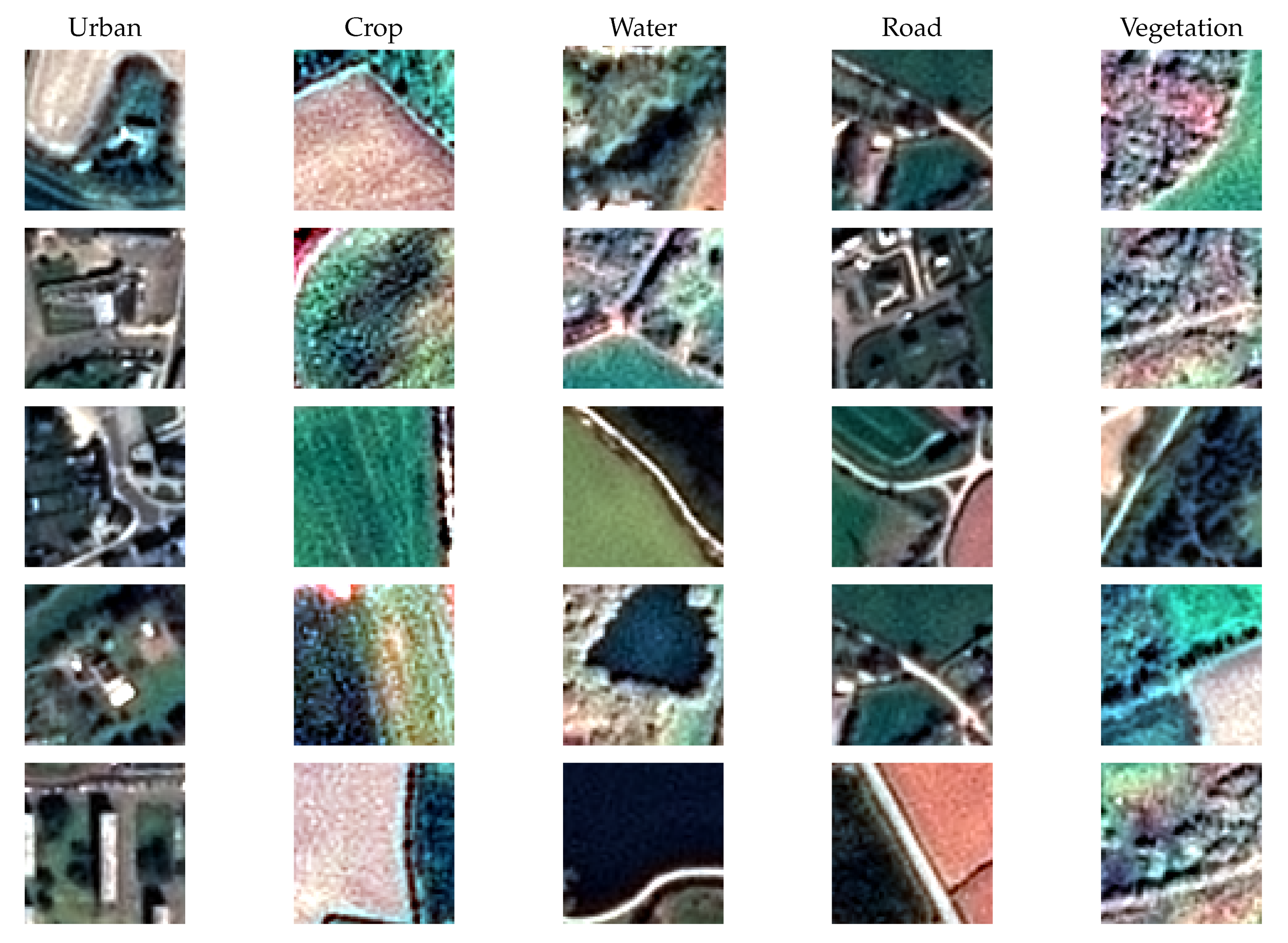
This study also provides an in-depth analysis of the performance of the various land cover classes in different types of landscape, which may guide the selection of an appropriate methodology in land cover classification over wide areas. These issues are illustrated with experiments on two very different land cover mapping problems, that have recently been addressed with CNN models. The first problem involves classifying 17 land cover classes using high-dimensional time series of Sentinel-2 multi-spectral images, while the second problem has a five-class nomenclature, and is based on imagery at a higher spatial resolution of 1.50m from the SPOT-7 satellite.
The detailed description of the HACCS method is provided in
Section 2. Then,
Section 3 presents the architectures of the two CNN models used in the comparison, as well as a discussion on their limitations. The experimental data set and the evaluation protocol used to compare the two approaches are shown in
Section 4, along with the results of the HACCS method. The interpretation of these results is discussed in
Section 5. Finally,
Section 6 presents our conclusions and insights on the issue.
2. The Histogram of Auto-Context Classes in Superpixels process
This study investigates the idea of describing the context of the target pixel using a prior prediction of the class labels of the neighboring pixels. The proposed method is named Histogram of Auto-Context Classes in Superpixels, abbreviated as HACCS. The different aspects and steps of the HACCS process are described in the three following sections.
First of all,
Section 2.1 presents the notion of contextual features, namely a group of methods called image-based contextual features. These directly use pixel values or calculate statistics upon the values of neighboring pixels in the image.
Next,
Section 2.2 presents stacked contextual classification methods. These first involve applying a prediction, or labeling step to the neighboring pixels, which allows the context to be described in a lower dimensional space than the initial pixel feature space.
Finally,
Section 2.3 explains why superpixels were chosen as a spatial support, and how they can be extracted from high-dimensional images which cover wide areas.
2.1. Image-Based Contextual Features
At submetric spatial resolutions, features such as the Scale Invariant Feature Transform (SIFT) [
22], the Speeded-Up Robust Feature (SURF) [
23], or more recently the Point-Wise Covariance of Oriented Gradients (PW-COG) [
24], aim to describe the context of a pixel by characterizing high spatial resolution features, such as sharp gradients and local extrema in the vicinity. This is achieved by extracting so-called keypoints, which are meant to characterize the points of interest in the image, and should help describe its content. This way, a pixel can be characterized by statistical information regarding the keypoints in its surroundings.
Another popular contextual feature for the classification of High Spatial Resolution (HSR) imagery is the Extended Morphological Attribute Profile (E-MAP) [
25]. This contextual feature is based on a series of mathematical morphology operations, namely closing and opening by reconstruction. The E-MAP describes the scale at which a pixel in the image is distinguishable from its neighborhood, and whether the pixel is generally lighter or darker than its surroundings. Other morphological attributes also describe geometrical properties such as elongation and squareness.
The issue with the previously mentioned features (SIFT, SURF, PW-COG, E-MAP), and with many other image-based features that are not mentioned here, is that they describe the spatial support in a very high dimensional space. For this reason image-based contextual features have limited applicability to land cover mapping based on high-dimensional imagery.
2.2. Local Class Histograms as a Contextual Feature
Most image-based features (SIFT, SURF, E-MAP) describe the spatial support in a dimension proportional to the number of pixel features, which is prohibitive for application on multi-spectral time series or hyperspectral imagery, for example. For this reason, unsupervised dimension reduction methods, for instance Principal Component Analysis (PCA), Independent Component Analysis (ICA), have been used before in studies on hyperspectral imagery [
26,
27,
28]. However, there is no theoretical guarantee that the relevant information for distinguishing the target classes is contained in the dimensions or linear combinations of dimensions with the highest variability in the data set.
Ideally, the reduction in dimensions should be guided by the classification problem at hand. This is the motivation behind stacked classification methods, which are based on a projection of the high-dimensional pixel features into a lower dimensional label space, using either a supervised classification scheme, or an unsupervised clustering technique.
For instance, the Bag of Visual Words (BoVW) method [
29], consists in applying
k-means clustering to a set of SURF keypoints, in order to extract a dictionary of so-called visual words. These represent different spatial features, such as corners or a local extrema. Then, the histograms of these visual words are calculated within a spatial support to be used as contextual features. The histogram can also be calculated on an entire image, for instance for image classification or for image matching [
30]. An unsupervised approach is used because an extensive nomenclature to characterize each of the low level classes in the image is impossible to obtain. Another reason for using clustering is that keypoint features and texture features often present very large dimensions, and clustering reduces the dimension of the contextual feature to the size of the visual dictionary.
Stacked classification methods can also use a supervised labeling, as is done in [
31], where an RF is used to classify the keypoints, and the scores from the various trees in the RF are then used by a SVM classifier. Here, in order to preserve the applicability to high-dimensional imagery, keypoint extraction methods are avoided.
Stacked contextual classification methods use the fact that the systematic errors of a pixel-based classifier can help characterize context-dependent classes. A pixel-based prediction is made with no knowledge of the context, and therefore contains certain predictable sources of errors, which can be learned in the successive iterations. For example, in land cover mapping, the combination of any artificial class and vegetation class in the same histogram serves as a strong indicator of the presence of discontinous urban cover.
The idea of using the result of a supervised classification to provide contextual information as an input to a classification model is essential to the Conditional Random Field (CRF) methods [
32,
33]. These methods involve using the estimated class-conditional probability density functions in a
neighborhood surrounding each pixel to build a context-aware model by minimizing energy functions to enforce coherence with the transitions observed in the training data set.
Another group of methods, known as the Semantic Texton Forests (STF) [
34], involves using a great number (millions) of features to generate the splits of the Random Forest. These features are simple functions of raw image pixels within a sliding window around the target pixels: either the raw value of a single random pixel, or the sum, difference, or absolute difference of a random pair of pixels. The optimization of the purity criteria guarantees the use of relevant features that best split the training data. Random pixels and pairs of pixels in the neighborhood provide a contextual characterization, in a way similar to how the CNNs consider the different combinations of neighboring pixels through convolutions. In a second step, the histogram of the tree responses and the histogram of the split nodes are calculated in a neighborhood (sliding window [
34], or object [
35]), and these are used as features for the final classification.
This is similar to the Auto-Context method [
36,
37]. In these studies, each pixel is classified using a number of image-based features, namely, color and texture features. While the initial classification is coherent, it lacks fine geometrical details in corners, and has the tendency to blur out sharp elements. In their study, the authors use successive iterations of classification using the same classifier and training data, but add supplementary features based on the predictions of the previous iteration. Specifically, the mean of the vector of class probabilities provided by the classifier, in several regions surrounding the pixel is used. As there are only two classes, this represents a very low total number of extra features, which allows a large number of different neighborhoods to be considered simultaneously, and for the pixel and image-based features to be preserved throughout the process. Selecting the shape and location relative to the target pixel of these neighborhoods carefully allows different aspects of the problem to be learnt by the classifier, for instance, spatial relations between classes, or relative positional information. The authors concluded that applying the Auto-Context algorithm several times refined the details of the geometry and improved the quality of the output classification. In fact, a large number of iterations was not seen as necessary, as the authors observed no more notable changes in the results after 5-6 iterations. This means that the process is light and fast, and potentially applicable to classification over wide areas with high-dimensional imagery.
The STF and Auto-Context methods address a similar problem as the one encountered in land cover mapping over wide areas, namely, the difficulty of classifying context-dependent areas while preserving the sharp corners and fine elements, on a large dimensional data set. Nonetheless, there are several differences between these methods and the HACCS process.
First of all, a normalized histogram of the predicted labels is used rather than the output probability vector of a soft labeling classifier, in a similar way to the histogram of clusters used in the BoVW features. Second of all, rather than using sliding window neighborhoods as in [
34,
38,
39], or more recently in [
40,
41], superpixels are used as spatial support to calculate the class histograms.
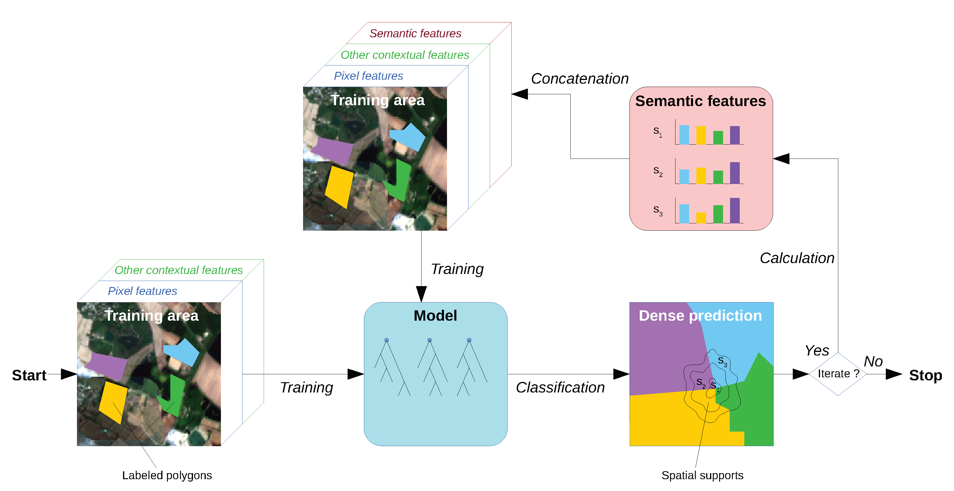
Figure 1 shows the different steps of the HACCS process. By using pixel features, optionally in combination with other contextual features, an initial classification model is trained. This model is then used to achieve a first dense classification of the image. Once all of the pixels in the image are labeled, the histogram of these predictions is calculated in each neighborhood, and used as a contextual feature. In the HACCS process, image-based features can optionally be used to generate a more accurate estimation of the first dense classification map. They can be useful for improving the quality of the first classification, and for providing complementary contextual descriptors to the histogram of classes. These optional features are represented by the green box labeled “Other contextual features” in
Figure 1.
The methods cited above can be described by five properties, given in the following list.
The density of the initial prediction: certain methods predict the class or cluster of keypoints, whereas others use every single pixel in the image.
Supervised or unsupervised prediction: some methods prefer the use of clustering rather than supervised classification for the initial prediction.
The contextual features, or lack thereof, used for the initial prediction: the first prediction can be pixel-based, or can already be based on the use of pre-selected contextual descriptors.
The number of iterations: certain methods stop at the second prediction, while others use successive predictions to improve the classification in an iterative way.
Adaptive spatial support. The definition of the context can be a sliding window, or an adaptive spatial support.
Table 1 shows the characteristics of the different methods that were cited previously. Clearly, the nomenclature of the different methods is not very well defined, as they originate from a variety of backgrounds and applications. None of the methods possess all five of the characteristics.
Table 1 also shows that the the HACCS method can in some cases bear all five of these properties.
2.3. Multi-Scale Superpixels as Spatial Supports
The choice of which spatial support to use to calculate the histogram of the class labels is not a simple one. Two commonly used spatial supports used for calculating contextual features are sliding windows and objects [
19].
Previous studies on the geometric precision of land cover mapping have shown that the use of a sliding window neighborhood with a so-called unstructured feature can increase the risk of blurring out high spatial frequency image features [
43]. Unstructured features do not take into account the spatial arrangement of the pixels in the neighborhood. Other examples of unstructured features are the sample mean and variance. In fact, this phenomenon is observed on experiments on the Sentinel-2 and SPOT-7 datasets, shown in
Section 4.
The other popular spatial support is the object, which is the result of an object segmentation method such as Mean Shift [
44], or Region Merging [
45].
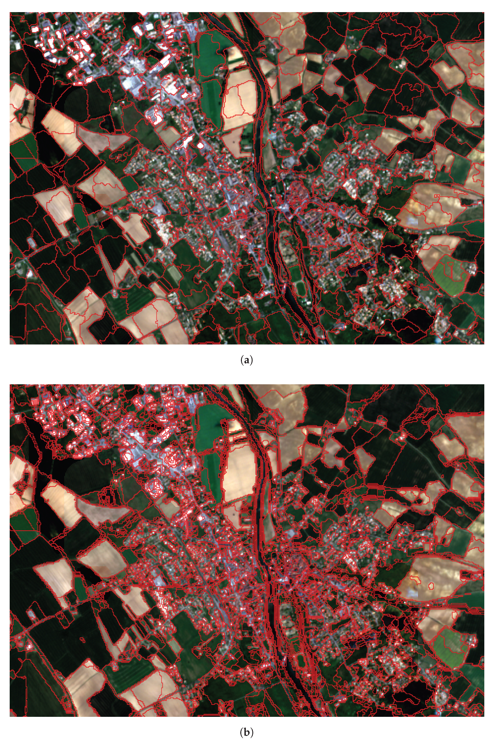
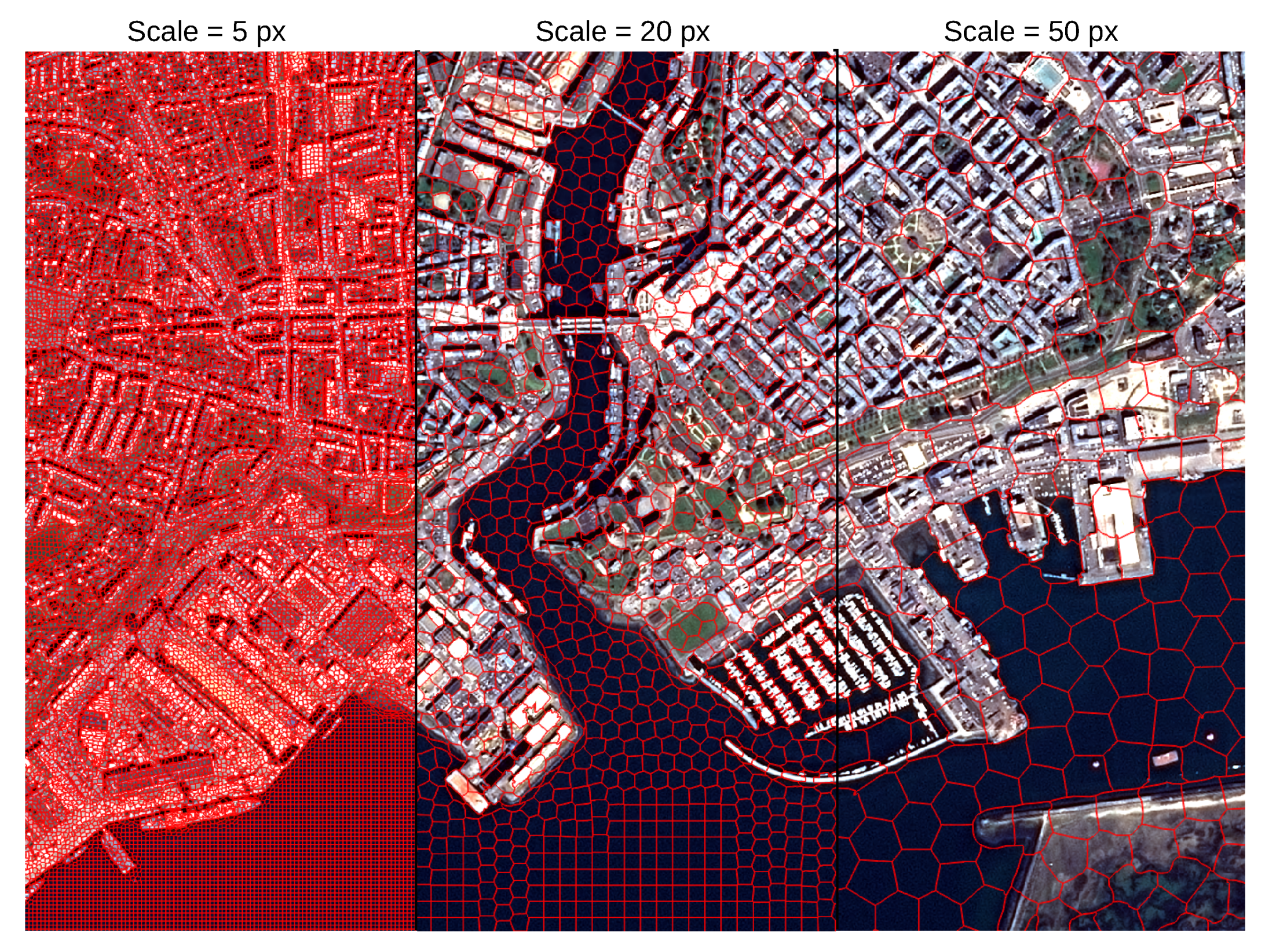
Figure 2b shows that in highly textured areas such as urban areas, the Mean Shift segmentation algorithm fails to provide segments containing diverse pixels. Therefore, a different type of segmentation is used here: superpixel segmentation. The algorithm used in this study, known as Simple Linear Iterative Clustering, or SLIC [
46], aims to provide segments that exhibit homogeneous features, but are also similar in size, and have a relatively compact shape, as is shown in
Figure 2a.
This algorithm is also very fast, and can be applied to remote sensing imagery over wide areas, using the scaling method described in [
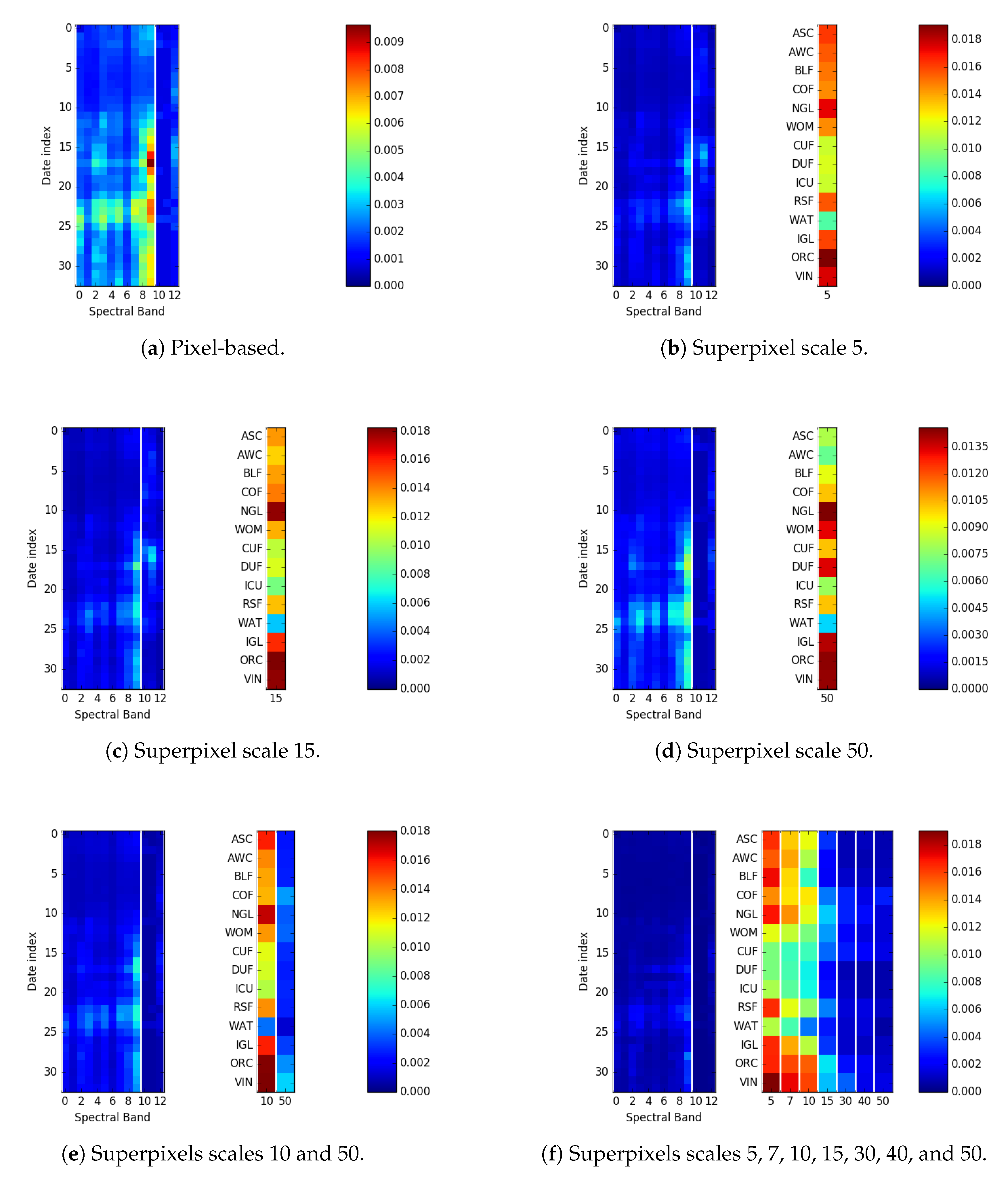
47]. The size of the grid at the first iteration of the SLIC algorithm is a parameter which is set manually, and which conditions the average size of the superpixels in the final segmentation. This parameter is referred to as the scale of the superpixel segmentation. The scale of a superpixel segmentation can be seen a characteristic diameter, in other words, the square root of the average area of the segments. This parameter gives an indication of the average distance at which contextual information is considered.
The choice of which scales to use depends on the application, in particular, which context-dependent classes are targeted, as well as the spatial resolution of the images. Initial experiments on the HACCS process indicate that using histograms in several scales of superpixels is beneficial compared to using only one. Indeed, it seems reasonable that a multi-scale description of the neighborhood would be useful for characterizing context-dependent land cover classes.
The scale of the superpixels is a parameter of the HACCS process, which can be selected according to a priori knowledge of the target classes, through experimentation, or both.
5. Discussion
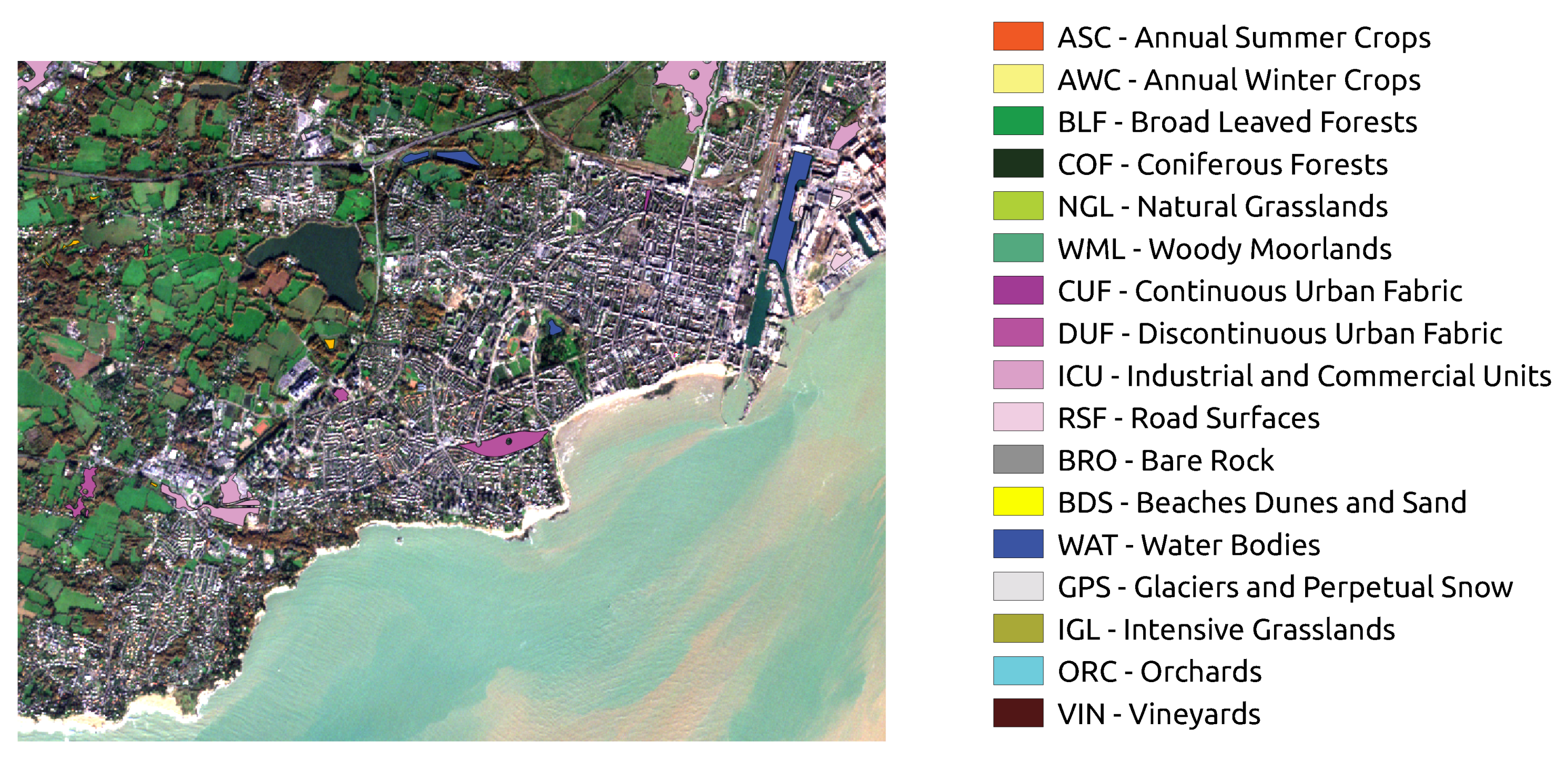
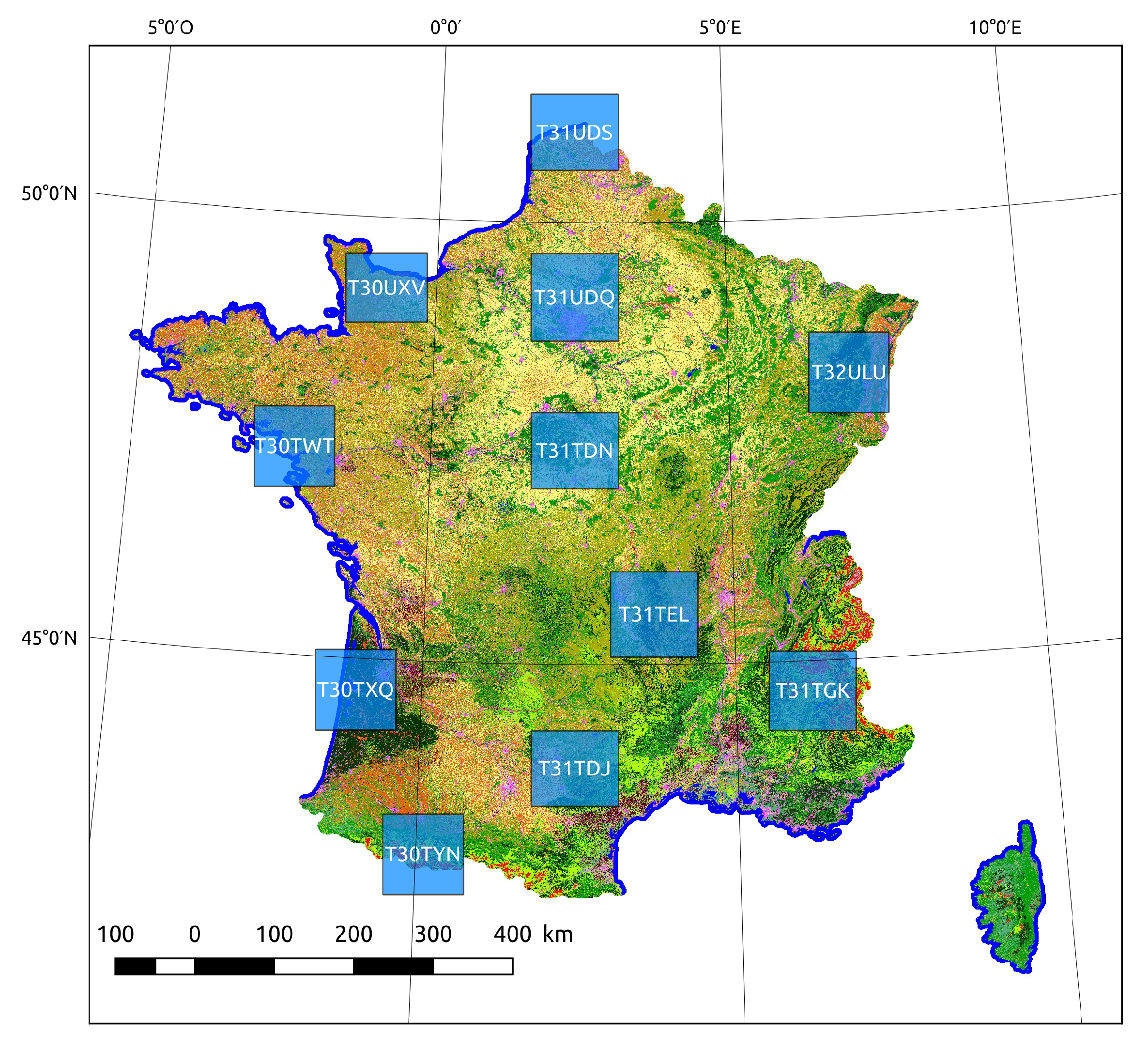
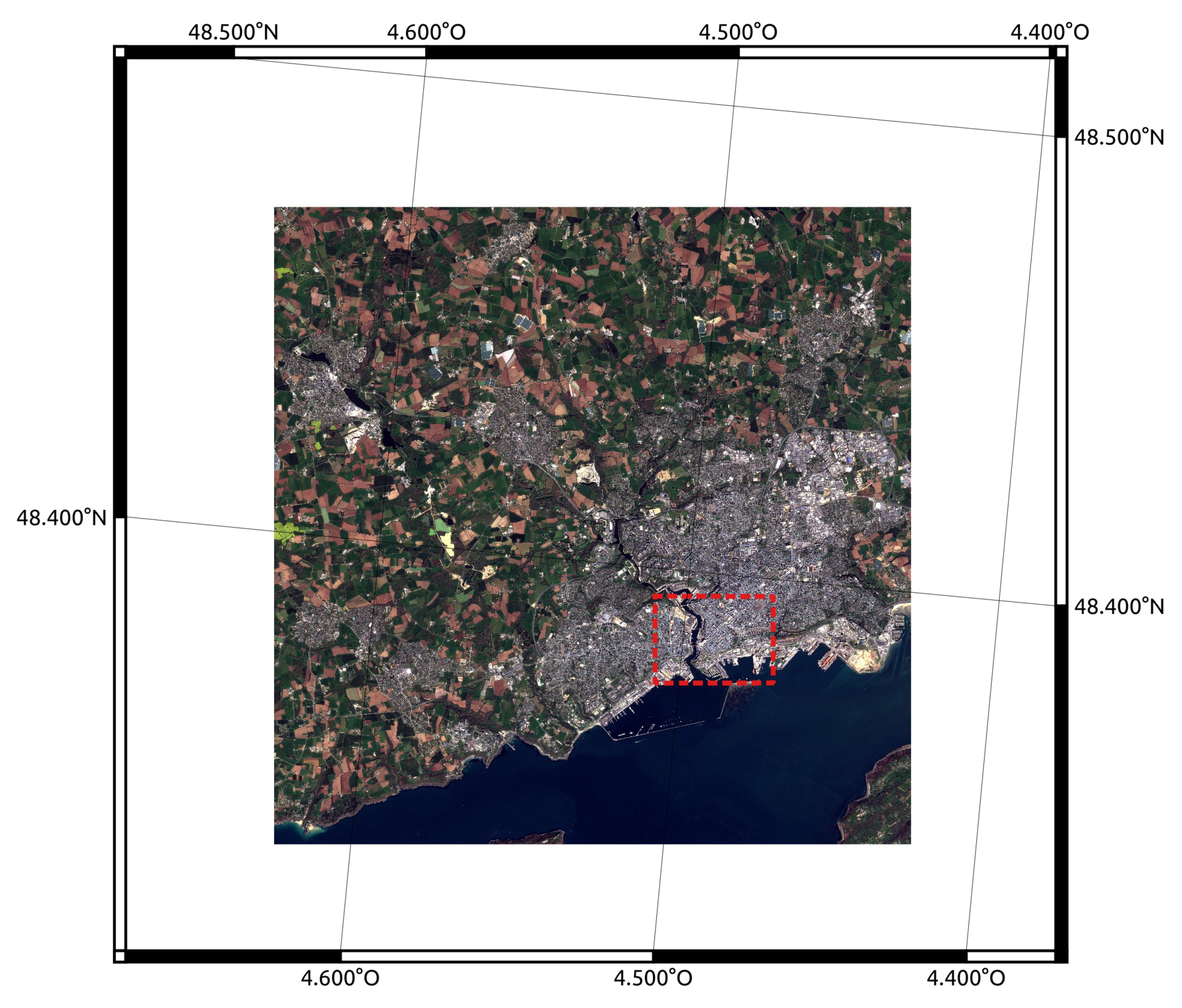
The first classification problem, presented in
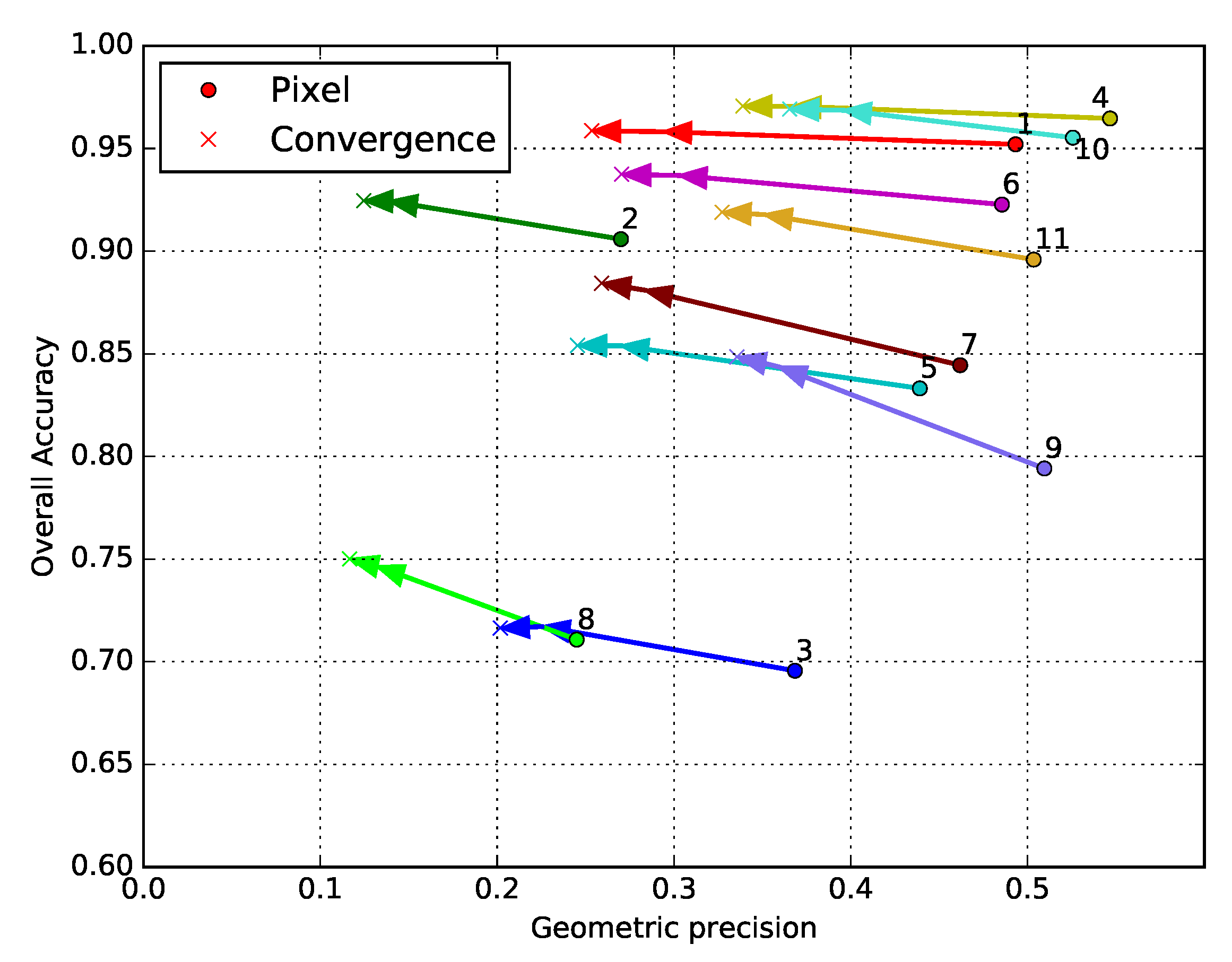
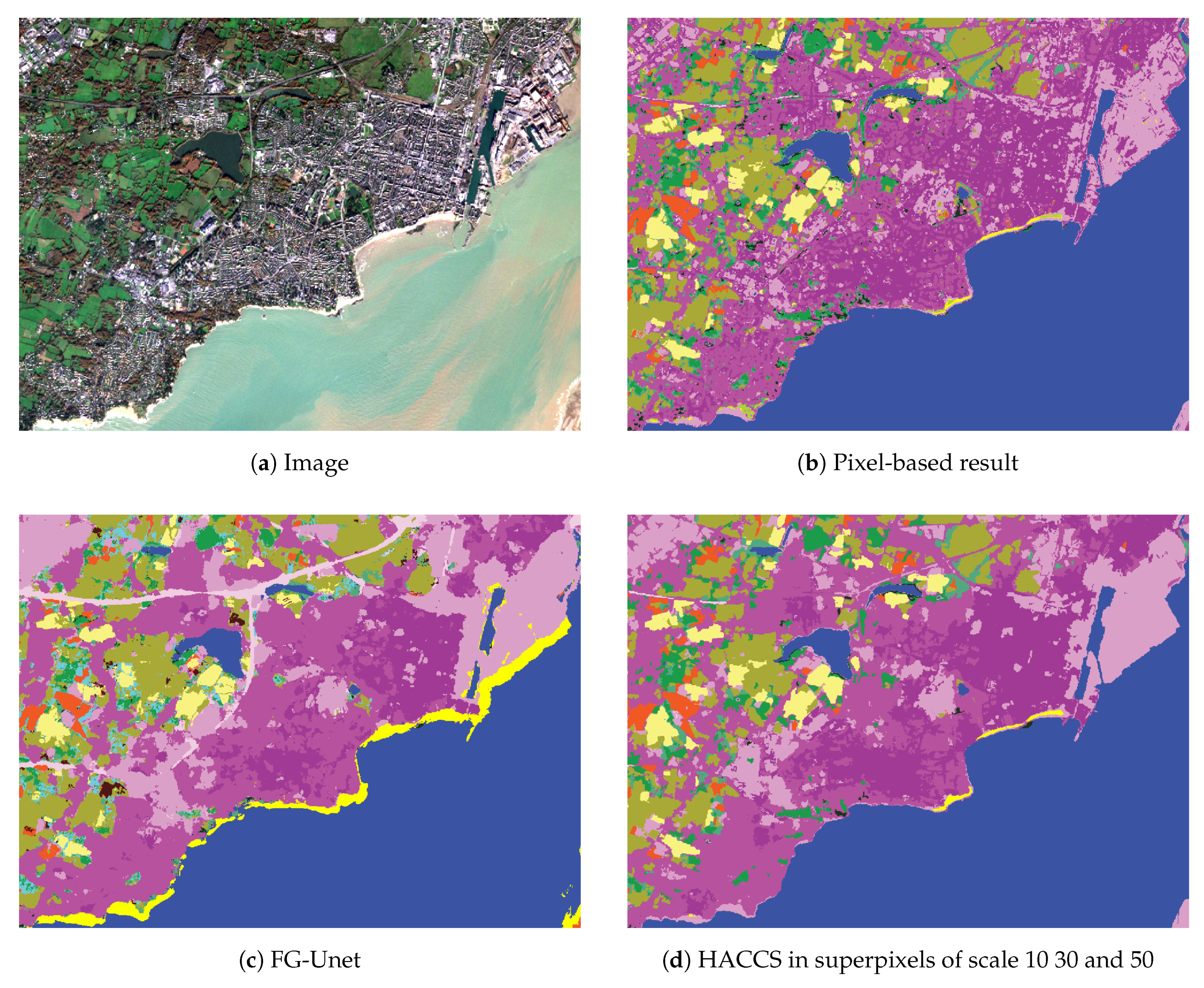
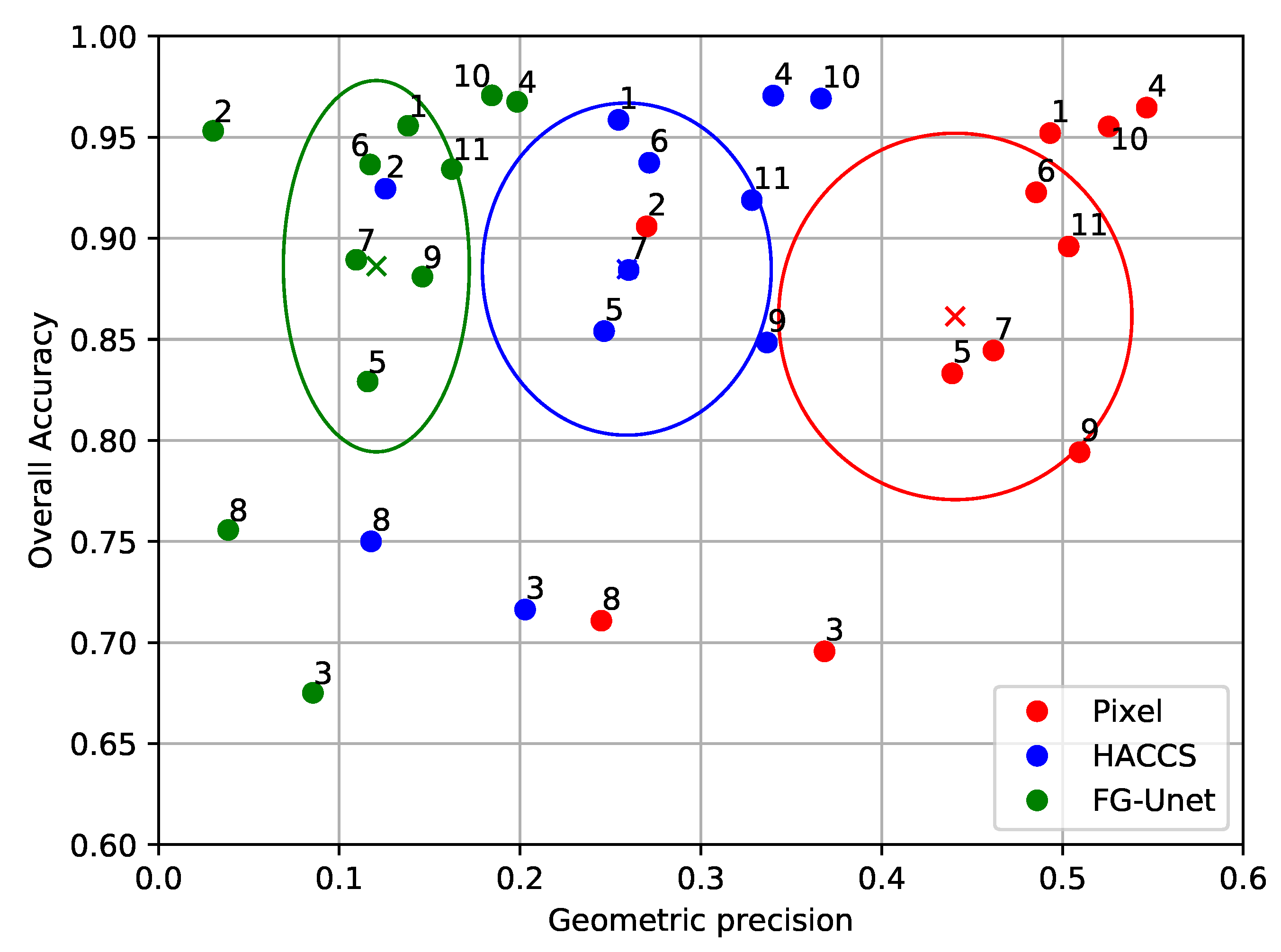
Section 4.2, is a land cover mapping problem over 110 × 110 tiles covering parts of the French territory. The use of 10 m spatial resolution Sentinel-2 time series enables a variety of natural, agricultural, and artificial classes to be recognized using supervised classification methods. Training data for these methods almost always come in a sparse form, which is why this case study is representative of a real world land cover mapping problem. Moreover, high-dimensional time series are rarely used in combination with contextual features, due to limitations in the total number of features that can be simultaneously considered by a supervised classifier. The main advantage of the HACCS process is that it does not require very many features. Indeed, the number of features is conditioned by the class nomenclature and the number of scales, and not by the type of imagery, making it adapted for classifying images presenting a great number of original pixel features. The experiments on this data set show that the HACCS process provides a similar performance to the CNN architecture in terms of overall accuracy. Moreover, the HACCS process produces maps with a higher geometric accuracy, measured by how well the classification can restore sharp corners compared to a pixel-based classification. This result is consistent across 11 Sentinel-2 tiles, which each cover an area of around ten thousand square kilometers, meaning that the proposed method is relatively robust to differences in class proportion and land cover class behavior.
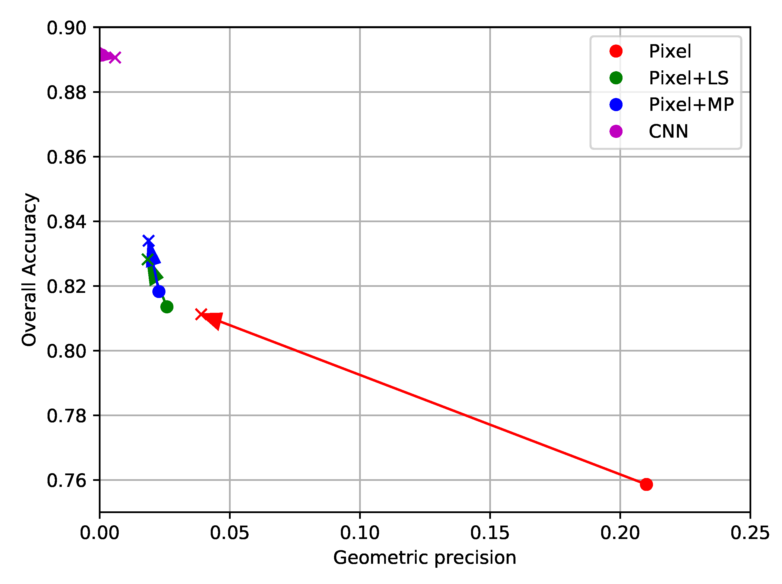
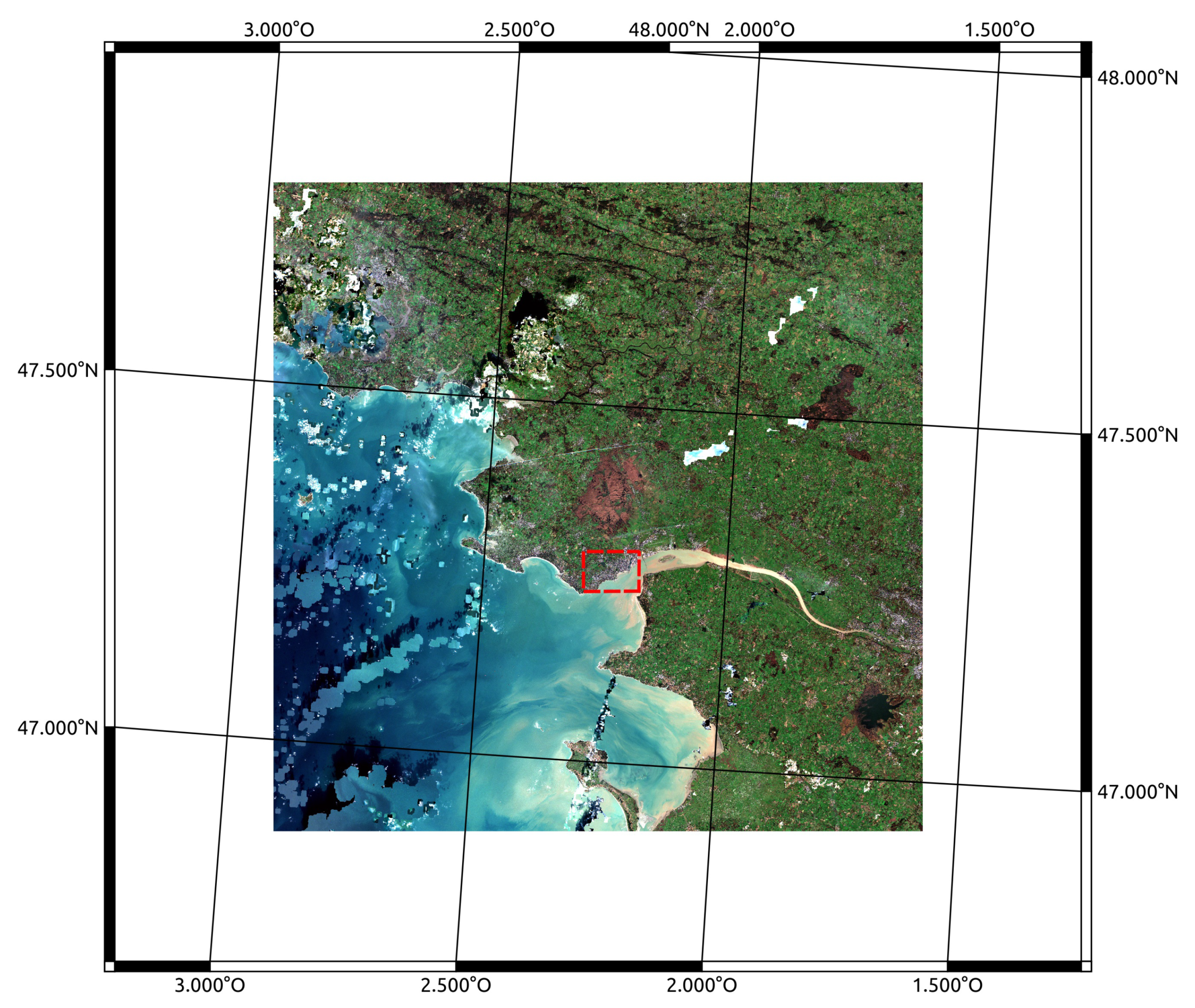
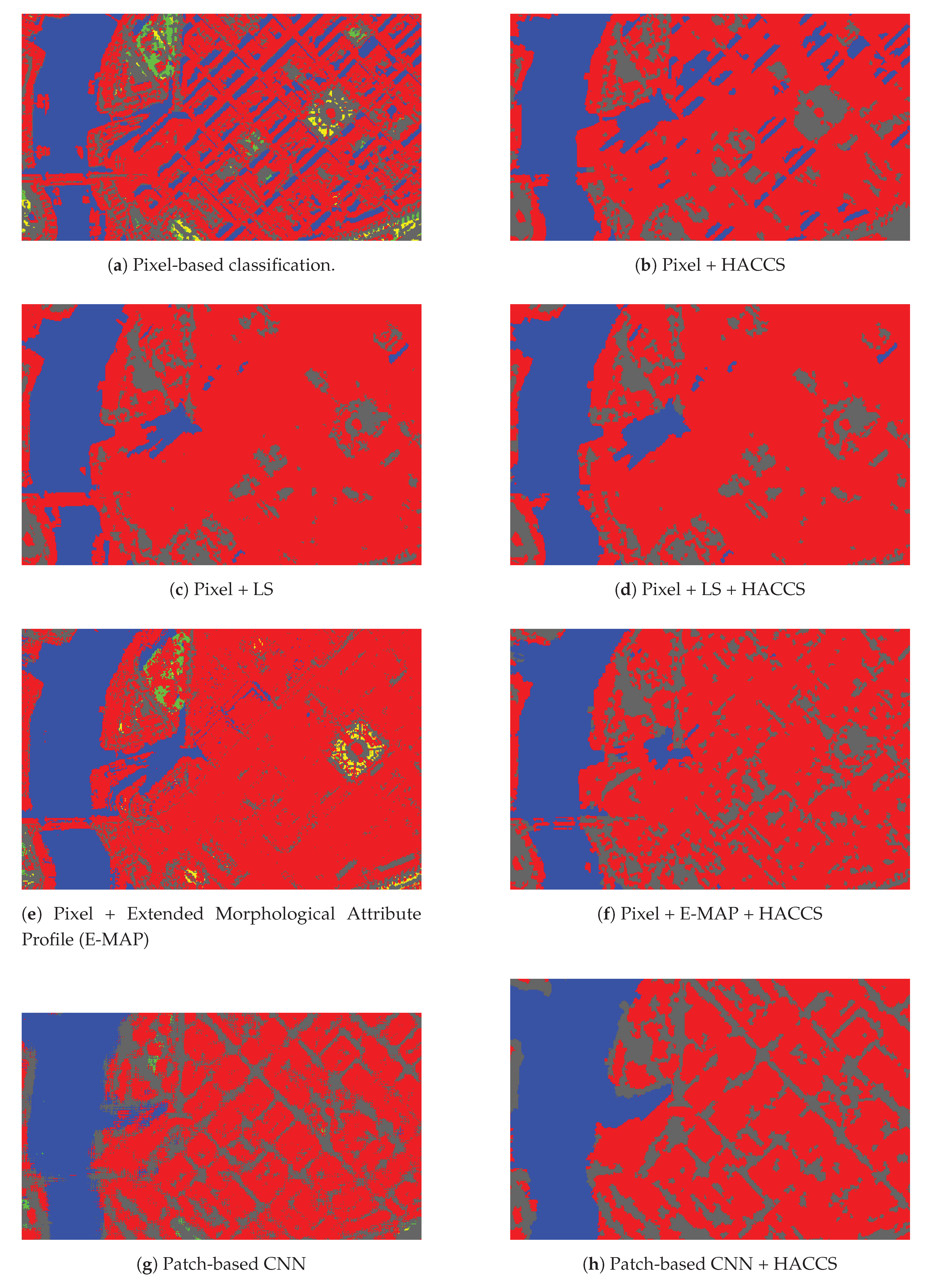
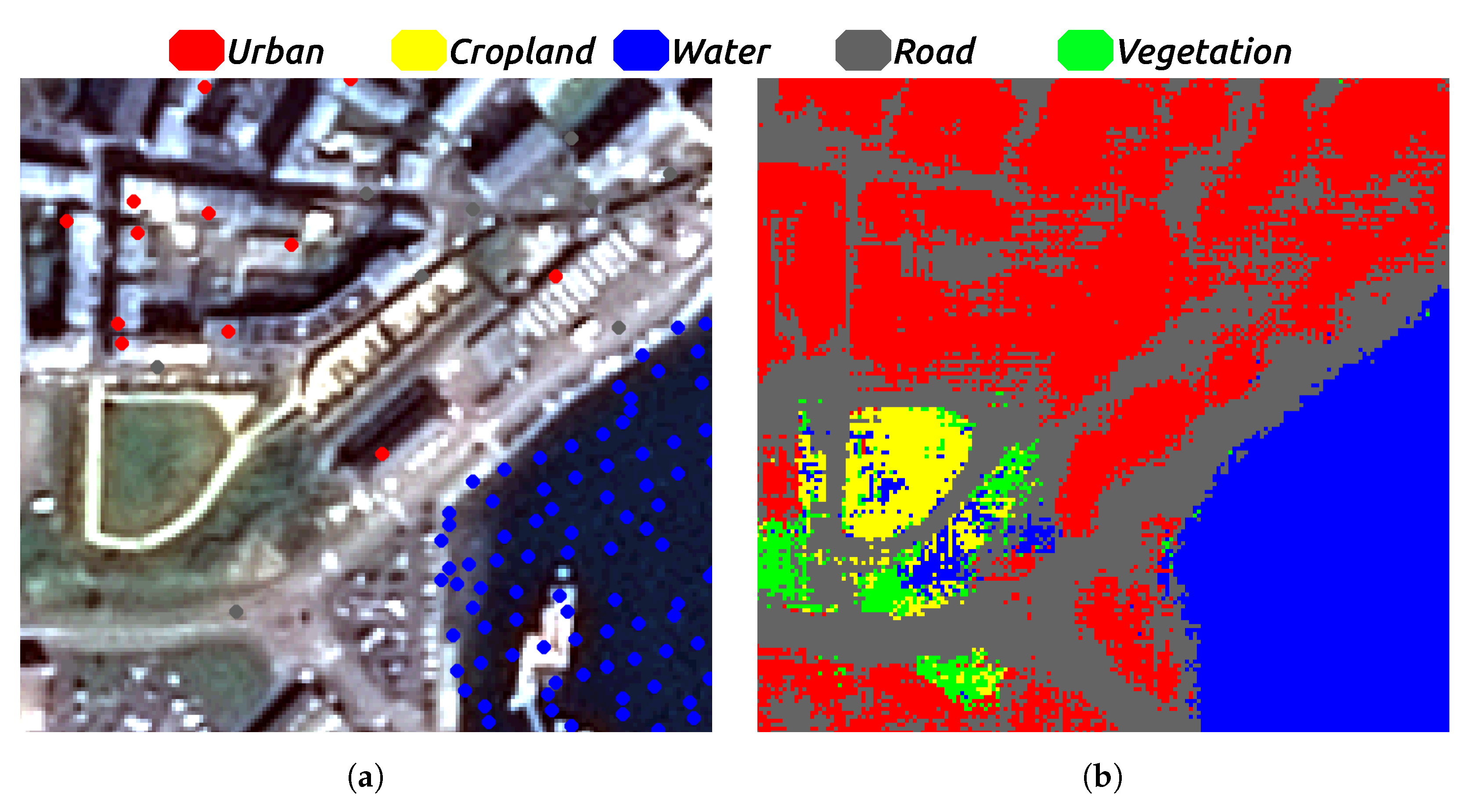
Next, the same methods are applied to imagery from SPOT-7. Unlike the Sentinel-2 time series, these images are mono-date, have a far finer spatial resolution of 1.5 m, and have a lower spectral resolution with only three visible bands and one infrared band. This implies that each pixel originally contains a relatively low number of features, however, more pixels are required to cover an equivalent zone. Two groups of standard contextual features are evaluated on this problem: the Local Statistics (LS), which contain sample mean, variance, and edge density, and Extended Morphological Attribute Profiles (E-MAP). Alone, the E-MAP features provide both the highest values of OA, with similar values of PBCM as the LS features.
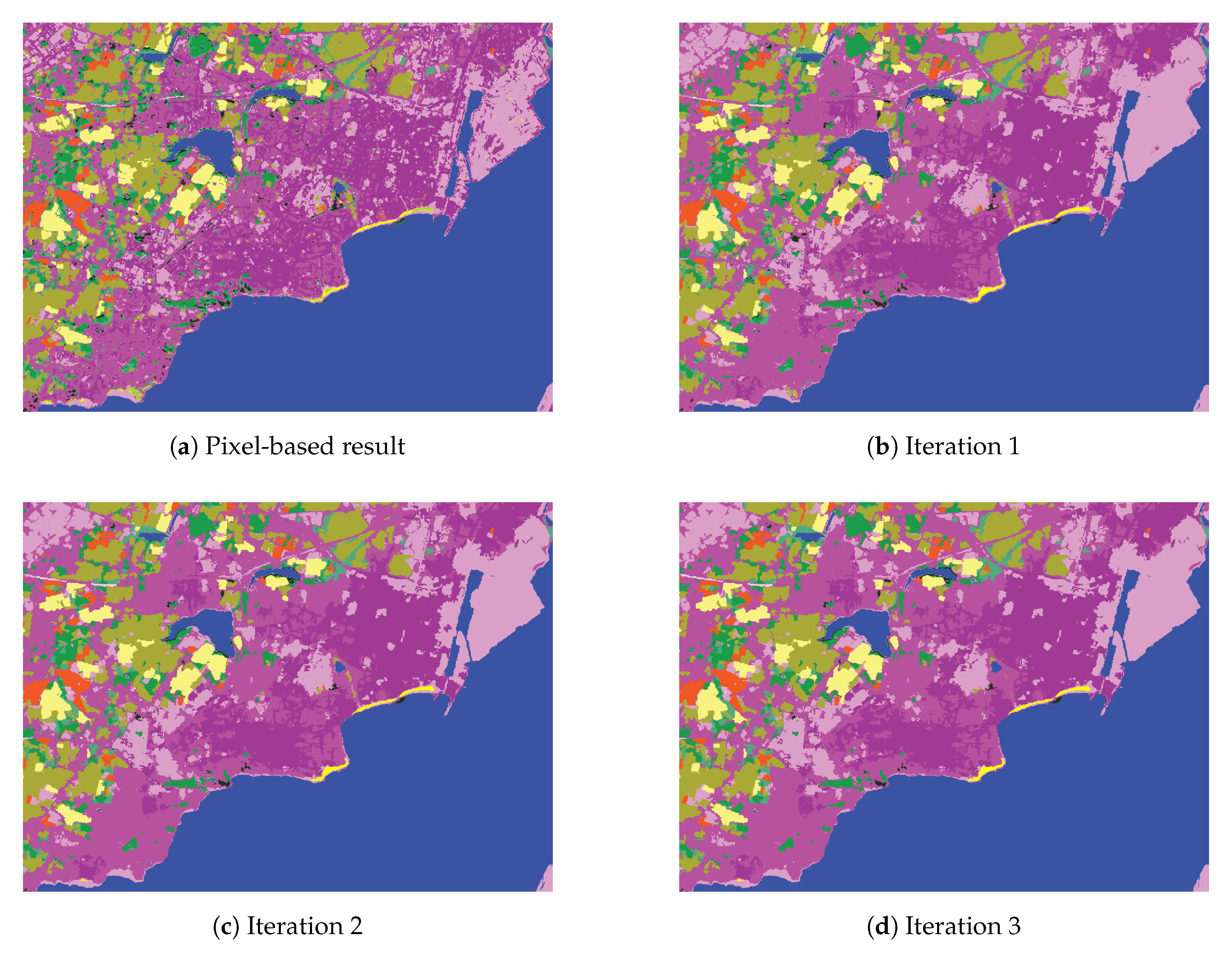
Then, experiments are run where the histograms are based on a classification result that is already generated with contextual features. Using several iterations of HACCS in multiple superpixel scales allows for a consistent improvement of the precision of each class. However, some of the corners present in the pixel-based classification are displaced or lost. When comparing these results to the classification map generated by the patch-based CNN from [
50], it appears that the handcrafted features (LS, E-MAP, HACCS), provide lower values of overall accuracy on this problem. Indeed, very high spatial resolution problems with a low number of image features are similar to the Computer Vision problems for which these networks were originally designed. On the other hand, the handcrafted features generally show a higher degree of geometric precision, in other words, they contain well localized sharp corners. This is both visible in the classification maps, and quantified by the experiments run on this data set.
The results presented in
Section 4.3 show that the HACCS process generates a pertinent contextual description, even for low-dimensional images at a higher spatial resolution. Alone, HACCS provides comparable results to other contextual features like local statistics and Extended Morphological Profiles. When combining the HACCS process with the standard contextual features, the classification accuracy after a few iterations is significantly improved. However, on this type of mono-date high spatial resolution imagery, the patch-based CNN does provide an overall more accurate classification result.
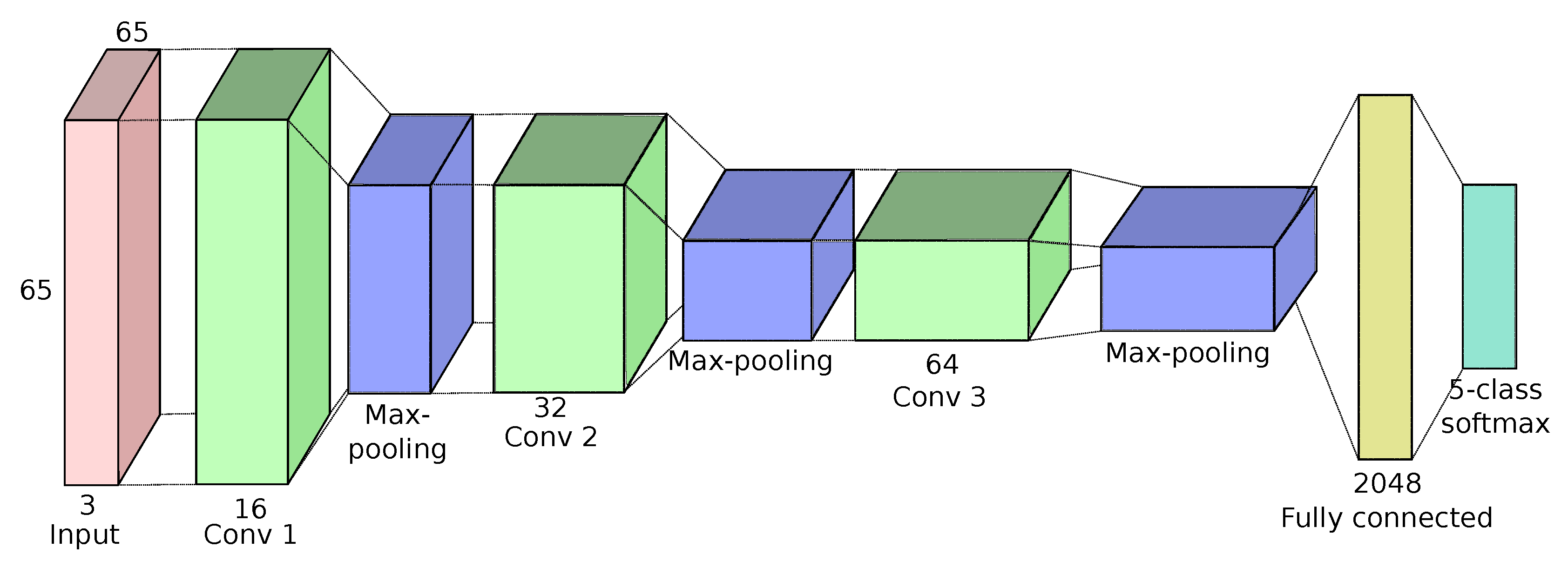
It can be noted that using a patch-based image classification network for semantic labeling, as was done in the SPOT experiments, is far from ideal, seeing as this is not the original purpose of these networks. However, we believe that there are other important aspects to this issue. Firstly, these patch-based networks have no requirement on the density of the labeled data: they can be trained even on data sets containing only labeled pixels spread very sparsely in the image, which does make them interesting candidates for such extreme cases. Secondly, it remains interesting to observe the results of such networks when applied to a semantic labeling problem. In fact, the SPOT experiments show that these networks do not totally fail, as one might expect. They have very strong detection capabilities, and are able to detect roads where methods using contextual features with adaptive neighborhoods are unable to. Their main issue seems to be in precisely localizing the edges of objects. Thirdly, there have been experiments on very high spatial resolution imagery (Pl∖’eiades) which have shown that even fully-convolutional architectures such as Unet also have issues in providing results with an accurate geometry, particularly when faced with noisy training data sets, and that this effect is reduced when fine-tuning the network with manually corrected data [
6].
6. Conclusions and Perspectives
In this paper, the Histogram of Auto-Context Classes in Superpixels (HACCS) process is evaluated as a new method for generating land cover maps with context-dependent classes, in the absence of dense training data. The contextual feature that is used is the histogram of class predictions, in one or more superpixels [
46,
47] of different sizes. These predictions can either be taken from a pixel-based classification or a classification with contextual features, which allows the method to operate starting with any classification result, and iterated several times, as is shown in
Figure 1.
This method is compared to the current state-of-the-art methods for including contextual information in dense classification schemes, Convolutional Neural Networks. The architecture of these networks is designed to take a patch of pixels as an input, which allows for an end-to-end optimization of both the feature extraction and feature selection steps.
Overall, in these two very different land cover classification experiments, the use of Convolutional Neural Networks seems to provide lower degrees of geometric accuracy than superpixel based methods with handcrafted features. This may be due to the sparsity of the training data, which are insufficient to describe the geometry of the objects during training. In other words, the neural network is not discouraged for generating results with smooth corners, as these corners are absent from the training data, and therefore from the loss function. On the other hand, superpixel-based methods extract the geometry of the objects directly from the image, which in many cases preserves the geometry. This conclusion must be taken with care as it is based partly on a visual validation and therefore is limited to the area that was analysed in detail.
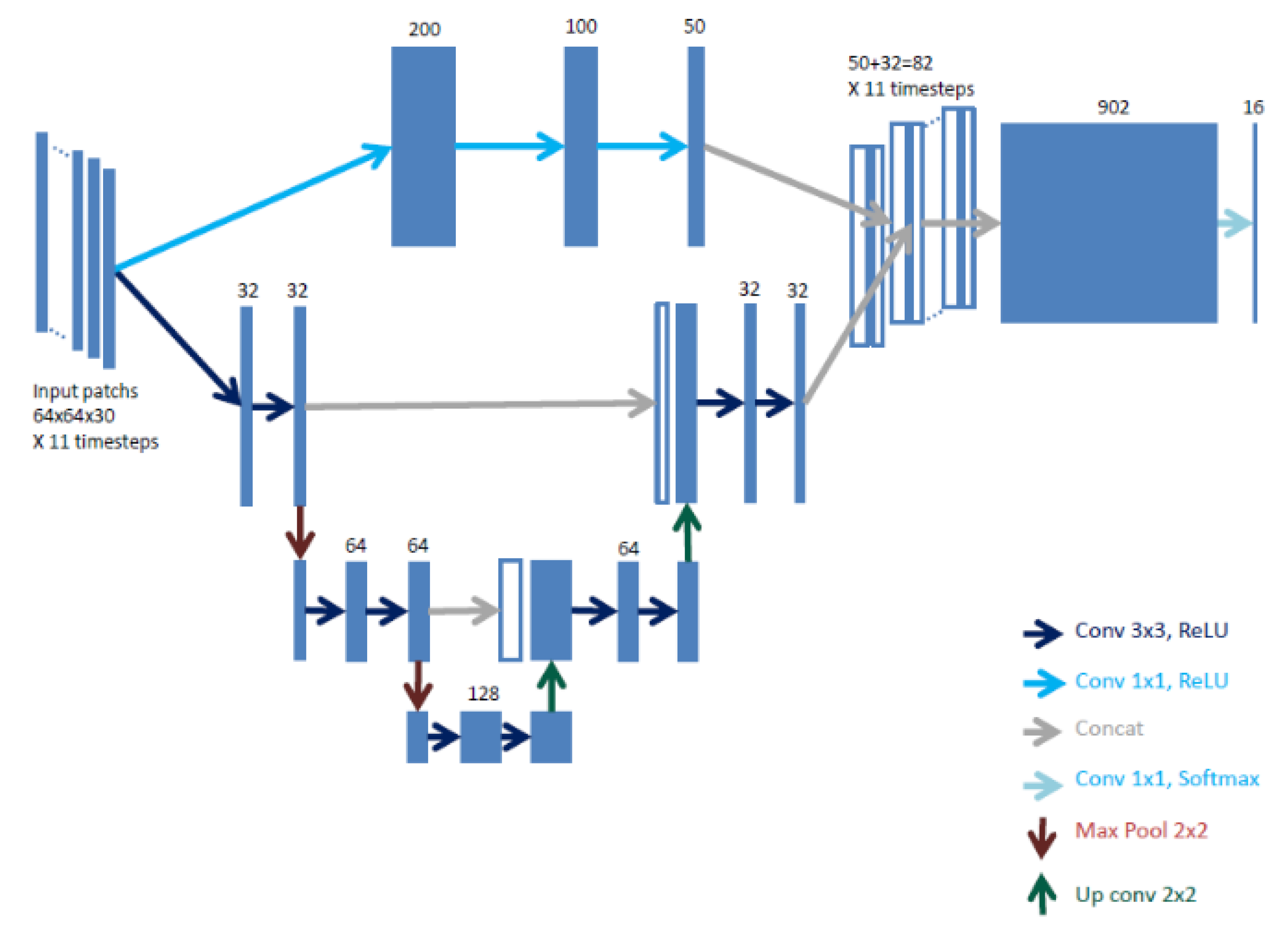
Secondly, in high-dimensional feature spaces, such as the time series used in the Sentinel-2 experiment, it appears the HACCS process provides results with equivalent levels of class accuracy as the FG-Unet architecture [
53]. Moreover, the HACCS results systematically present a higher rate of geometric accuracy, with a finer localization of sharp corners. It also is worth mentioning that the HACCS process is computationally lighter than neural networks, as it only involves the training of a Random Forest for each iteration, which is very fast in practice. It would be interesting to study whether these results can be extended to hyperspectral images that also present a very high number of image features.
Finally, when using images with similar characteristics to the ones encountered in Computer Vision problems, i.e., a very high spatial resolution, and a low number of features per pixel, the CNNs show the strongest levels of class accuracy. On the other hand, the geometry of the result is questionable, with the presence of speckle-like label noise near object boundaries, and smooth corners. Handcrafted features in superpixels, like HACCS, allow for higher levels of geometric precision. In further studies, it would be interesting to evaluate the effect of the density of training data on the geometry of the classification map, and the application of HACCS to other dense image classification problems, such as hyperspectral or radar imagery.
Overall, this study suggests that for the higher spatial resolution images with fewer features (SPOT-7) the use of CNNs may be preferred, under the condition that a higher computational cost and lower geometric accuracy is acceptable. Moreover, if HACCS is applied to such images it must be done with care, as if the number of contextual features largely exceeds the number of pixel features, it may result in a degradation of the geometry. For HSR imagery (Sentinel-2) with more pixel features, HACCS seems to be the preferred solution, seeing as it provides a similar performance with a lower computational cost.
The source code for the HACCS process is based on the use of the open source software Orfeo ToolBox, and is freely available [
68].


