1. Introduction
Unmanned Aerial Systems (UAS) extend the applications range of aerial imaging to various domains, due to efficient acquisition time, costs, and repeatability.
Structure from Motion photogrammetry (SfM) is the most used technique for UAS image processing, since, unlike traditional photogrammetry, the three-dimensional (3D) structure of an object is reconstructed based on two-dimensional overlapping image sequences without the need of ground control points (GCPs). The intrinsic and extrinsic parameters are automatically calculated based on image coordinates of common points (feature points) through bundle block adjustment (BBA), and a sparse point cloud is generated. This point cloud is densified using Multi View Stereo (MVS) techniques, the gross errors being removed [
1,
2]. Nevertheless, the main aspects of processing the UAS images remain image blocks orientation and georeferencing that can be simultaneously performed through BBA or independently. There are two important steps for BBA: automatic pairwise image orientation using RANSAC for robustly estimating relative orientation based on keypoints matches (the matches are filtered), thus estimating the relative orientation for all image pairs and the second stage can be done either incrementally, by creating the bundle block by starting with best image pair and iteratively adding one image, or applied globally. There are two methods for the georeferencing process: direct georeferencing of images by using the navigation sensors (mainly GNSS) [
3,
4,
5,
6,
7,
8,
9,
10] and the indirect georeferencing of images by using ground control points (GCPs).
Sanz-Ablanedo et al. [
5] centralized different studies regarding determining the direct georeferencing accuracy. The conclusion drawn from these studies is that the GCPs must be included in project design if a sub-decimetre is required in elevation accuracy.
In general, the cameras that are mounted on UASs are consumer-grade digital cameras having large radial and tangential distortions. Therefore, using the self-calibration in the process of orienting the image block, especially when having only nadiral images, will cause high errors in the process of surface reconstruction called dome effect [
11,
12] or bowl effect [
13]. These distortions can be estimated either by using GCPs [
12,
14,
15] or a pre-calibrated camera. As demonstrated by Oniga et al. [
13], when using a very high number of GCPs (e.g., 50), the results are similar for the methods of calibration: self-calibration and pre-calibration. Moreover, using a large number of GCPs the pre-calibration process improves the results with more than 50% in comparison with self-calibration, whereas for a minimum of three GCPs in the process of image block orientation and a pre-calibrated camera the accuracy is improved with more than 90%.
Taking all of the above in consideration, the ground control points can greatly increase the accuracy of the three-dimensional (3D) information and their measurement is an important aspect of georeferencing the UAS image blocks. Moreover, it was demonstrated that increasing the number of GCPs will lead to higher accuracy of the final results i.e., point cloud, 3D mesh, orthomosaic, digital surface model (DSM), or digital terrain model (DTM) [
16,
17]. Although, exceeding the number of ground control points is a time-consuming process, both in the field and computationally, finding a suitable number being of primary interest. Another important aspect is the impact of spatial distribution of GCPs and the accuracy of the georeferencing process.
In the last years, finding the optimum number of ground control points needed for a UAV flight was of prime interest to researchers, but in special for georeferencing the DSM [
17,
18,
19,
20,
21,
22], the orthoimage [
17,
19,
22,
23,
24,
25] and the point clouds [
26,
27] generated by processing the UAS images. Studies on the accuracy assessment of Structure from Motion (SfM) image block orientation have also been performed. Sanz-Ablanedo et al. research [
5] was conducted on an extended area of 1200 ha with 102 points, having both roles of GCPs and check points (ChPs), with a fix-wing UAV taking 2514 images, and the flight being taken at 120 m height above the flight control station with varying overlaps. It is concluded that, the RMSE will slowly converge to a value approximately double the average GSD (in their study 6.86 cm) of approximately ±16 cm by having more than 2GCPs/100 images (50-60 GCPs and 52-42 ChPs). On the other side, when using four GCPs/100 images (90–100 GCPs and 12–2 ChPs), the accuracy is about ±12 cm. It is noticeable that using only a low number of ChPs, the estimated statistical quantities may have a large uncertainty. Additionally, the general conclusion that is stated by Sanz-Ablanedo et al. [
5] cannot be applied on small projects, where less than 100 images are captured. Rangel et al. [
22] assessed the accuracy of DSM and orthophoto obtained by the SfM method testing 13 scenarios with 177 GCPs and ChPs. The flights were done over a natural area (open pit mine) at an elevation of 228 m with a rotor UAS. They recommend a uniform distribution of 18 to 20 GCPs per image block to achieve a highly accurate DSM.
Regarding the spatial distribution of GCPs, Sanz-Ablanedo et al. [
5] demonstrated that these should be evenly distributed on the study site, ideally in a triangular node grid, but finding a measure for defining the most suitable geometrical distribution of GCPs was not the subject of the research, with authors affirming that this topic requires further investigation. Rangel et al. [
22] studied the spatial distribution of GCPs relative to the image block (peripheral and internal), finding that the inclusion of GCPs inside the block does not substantially improve the planimetric error, but, in the case of altimetric errors, as the number of GCPs increases, the error decreases considerably. Moreover, the authors found that, for best results, a uniform distribution of GCPs inside the block with a horizontal separation of three to four ground bases (distance between two camera positions) must be assured. Martínez-Carricondo et al. [
28] investigated the effect of the number of GCPs and their spatial distribution. They found that it is necessary to place GCPs around the edge of the study area to minimize the planimetry errors and create a stratified distribution inside with a density of around 1.7 GCP/ha to minimize the altimetry errors.
Although there were several studies conducted during the last decade to determine a suitable number and spatial distribution of GCPs, no general rule was established and the question still remains, mainly because the accuracy of the final products obtained after UAS images orientation is influenced by different factors: camera’s focal length, ground sample distance (GSD), image block configuration, image resolution, dedicated software, UAS system configuration, and the accuracy of GCPs measurement, both in the field and on images [
18,
26]. Therefore, each study contributes to the improvement of the products that were obtained by UAS technology, with the subject being of primary interest for both researchers and practitioners.
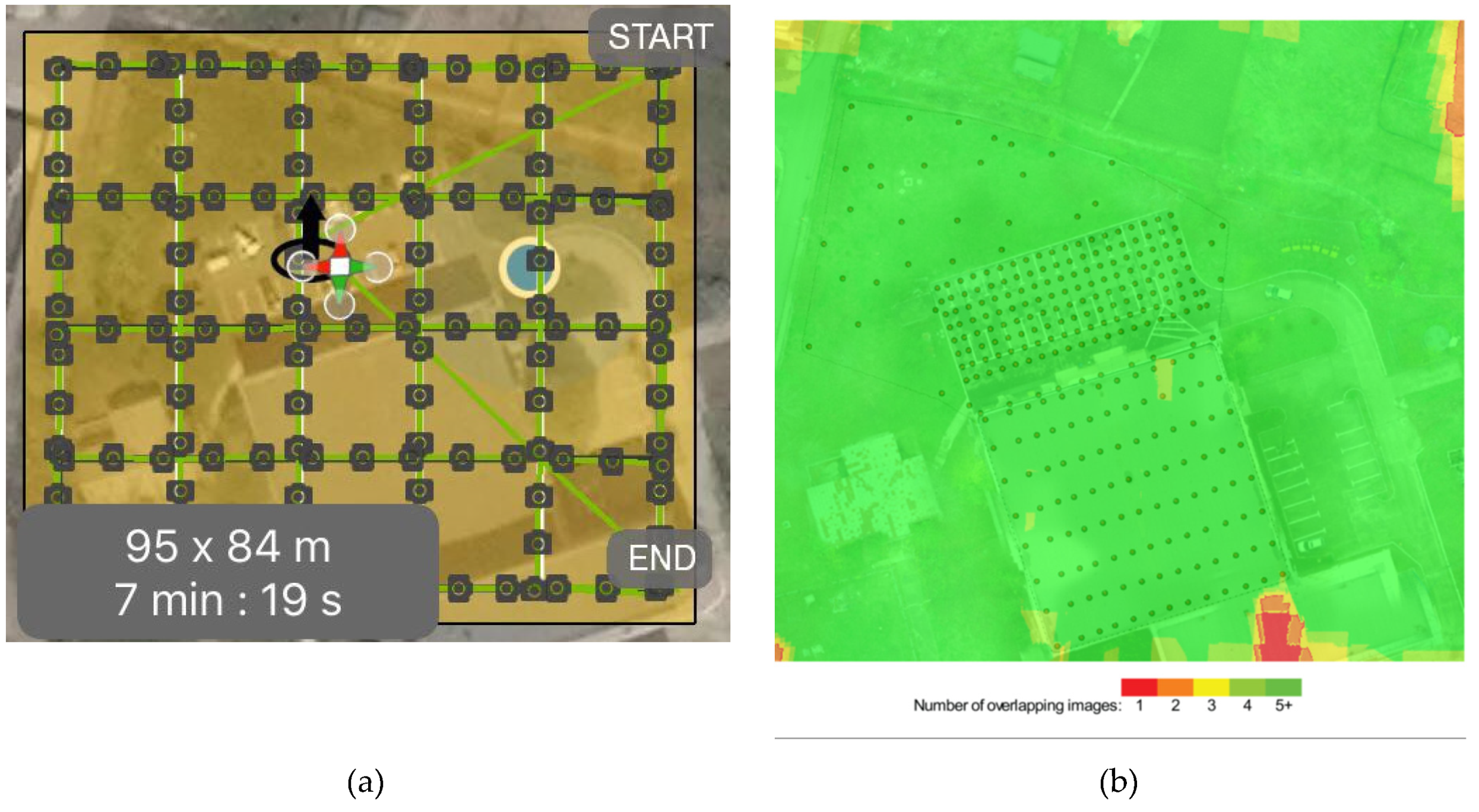
What differentiates our study from other related studies are: (i) the nadiral flight was made at a low altitude of 28 m to obtain a very high resolution, which is essential for urban area projects, with the GSD value of 1.1 cm being very small when compared with the above cited studies; (ii) the high number of targets used i.e., 150 GCPs and 150 ChPs with respect to the area covered by UAS images: 1 point/33 sq. m., the coordinates were determined with millimeter precision being independent of the deformations caused by the global geodetic systems due to the designed local geodetic network representing the first implementation made on an urban area containing artificial landscape e.g., building with uniform texture covering almost 15%, parking lot.
Taking two major factors that are influential and also flexible for an UAS project design, such as number of ground control points and their distribution, into account, the general purpose of the research is to find a rule that can be generalized for small UAS applications.
The acquisition was done at 28 m height and two approaches are derived for the spatial distribution of GCPs and ChPs, in different scenarios and while using 3DF Zephyr Pro software [
29] (that promises a lot in the 3D reconstruction area, which is commercialized by 3Dflow). The mentioned software utilized in the current research is not commonly used in scientific literature, with the most used being Agisoft PhotoScan Professional [
16,
20,
28,
30,
31]. The area of interest chosen for this study is 0.8 ha and it was photographed with a low-cost UAS, namely, the DJI Phantom 3 Standard, at 28 m height and a number of 300 ground control points and check points were measured using a total station.
4. Results
Four different scenarios were tested when only using four GCPs in the BBA (
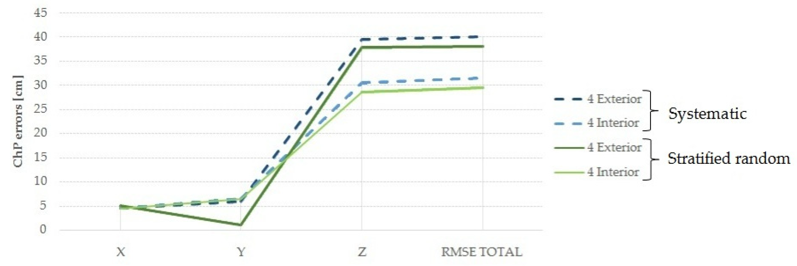
Figure 11). The study area has been divided in four and the corners have been marked with a rectangle. In each of the four corners, one GCP has been selected with respect to the interior of the rectangular boundary and with respect to the exterior part of boundary. Subsequently, 10 different combinations have been tested for the systematic distribution and, respectively, for the stratified random distribution.
The area covered by the 300 GCPs and ChPs was divided in four and the corners were defined by a rectangular boundary, as mentioned above. In each of the four areas, one GCP was selected while taking into consideration two spatial distribution: in the exterior part of the boundary and in the interior part, not too far out from the corners.
Table 1 lists the RMSE calculated for the 150 ChPs when using only four GCPs in the BBA process.
Figure 12 graphically represents the errors along the three axes for each scenario. Analysing the errors, the ChPs distribution has an influence on the residuals obtained, decreasing in both cases: for systematic distribution from 40.2 cm to 31.7 cm and for stratified random distribution from 38.2 cm to 29.6 cm. Nevertheless, the constant difference for RMSE
T of 8.5 cm between interior and exterior can be highlighted, for both cases, systematic and stratified random distribution, the differences in meters between the targets selected for GCPs exterior and interior distribution being approximately 6 m. The most suitable distribution of the four GCPs is obtained when the targets are located in the interior of the four corners.
It is noticeable that the vertical errors are six times larger than planimetric errors, directly influencing the total RMSE, the results being in accordance with [
26]. When comparing with the research that was conducted by Tomaštík et al. [
26], a few parameters were in common with the present study: low cost UAS system, image resolution, side-lap and end-lap, and size of the study area.
For the projects in which 8, 20, 25, 50, 75, 100, 125, and 150 GCPs, respectively, where used in the process of BBA, the errors along each axis have been computed: RMSEX, RMSEY, RMSEZ, along with the planimetric error, RMSEXY, and the total error RMSET.
Table 2 lists the RMSE calculated for the 150 ChPs when using a systematic distribution of the GCPs and the ChPs and
Table 3 lists the RMSE for the stratified random distribution scenario.
The planimetric values (RMSEX,Y) ranged between 2.0–4.7 cm for systematic and between 2.0-4.4 cm for the stratified random distribution, with the highest error corresponding to the eight GCPs scenario. It is mentionable that the differences between the two distributions are approximately a few millimetres, with a maximum of 3 mm. The vertical errors (RMSEZ) are varying for the systematic distribution between 3.7–29.1 cm, while for the stratified random one is between 3.6–19.1 cm, the highest error corresponding to the eight GCPs scenario.
Analysing the two distributions, the difference between the RMSET is 1 dm. The values are lower for the stratified random distribution, because the points are located on both the periphery and in the centre of the area. Moreover, while for the systematic distribution, the difference between four GCPs and eight GCPs scenarios is insignificant, only 2.1 cm, for the stratified random distribution is 1 dm.
The error tendency along all the tested scenarios along with the obtained result for each axis are presented in
Figure 13 for both distribution methods: systematic (a) and stratified random (b).
The graphic representations (
Figure 13a,b) highlight a deep drop of the RMSE
T between eight GCPs and 20 GCPs cases, being three times lower for systematic and two times lower for stratified random. In terms of GSD, for 20 GCPs, the accuracy is 3 GSD in planimetry, for both distribution types, and 7.9 GSD in elevation for systematic distribution and 7.4 GSD in elevation for the stratified random distribution. Increasing the number of GCPs with 5, the accuracy is the same for the systematic distribution and it improves with only 6 mm for stratified random. Adding 25 GCPs, the accuracy improves with approximately 2 cm for both distributions. The following scenarios, 75GCPs, 100 GCPs, 125 GCPs, 150 GCPs, follow a decreasing tendency of errors, but at a lower rate in terms of millimetres. By having a great amount of GCPs (i.e., 50 GCPs), the planimetric errors are almost the same while the vertical errors are lightly reduced.
Figure 14 individually highlights the spatial representation of the total root-mean-square-error of the check points for each scenario. It is noticeable the placement of both GCPs and ChPs for the systematic distribution (
Figure 14a) and the stratified random one (
Figure 14b) offers a more detailed analysis.
Analysing the
Figure 14, it can be seen that, for the ChPs situated on the roof edge and on the building façade, the errors are still larger when compared with the remaining ones, when using 20 GCPs or more. This was also the case of the Rangel et al. research [
22], where the errors tend to be clustered in areas with abrupt slope changes. They also mentioned that altimetric errors are located in areas with little texture and radiometric uniformity. This fact also represents a particularity of the current study, with the roof area having a uniform texture (light grey) extended on 0.13 ha.
In addition, the errors were classified according to their location in the four main segments of the study area, namely: roof, façade, parking lot, and green area (
Figure 15). Due to considerably large amount of generated data, based on the RMSE
T, the descriptive statistics were also listed in
Figure 15, taking all cases from four GCPs to 150 GCPs into the analysis. A decreasing central tendency of RMSE
T is clearly presented, being directly proportional with the variability, which, for all cases, shows a similar pattern, as described by
Figure 15.
The descriptive statistics expressed the best separation between the scenarios. Firstly, concerning the four GCPs scenario, the four interior-placed GCPs has a smaller variability having a mean of 0.27 m, median of 0.24 m for the systematic distribution, and a mean of 0.25 m and a median of 0.22 m for the stratified random distribution. In contrast, the four exterior-placed GCPs case shows a mean of 0.35 m and a median of 0.32 m for the systematic distribution and a mean of 0.33 m and a median of 0.30 m for the stratified random distribution.
Furthermore, the ChPs with high errors are located in the entire area, in all types of surfaces, natural or artificial, low and high altitude. In addition, the ChPs determined in the parking lot, which is located in the middle of the area, are influenced by the only ground control point marked on the right edge of it. The errors are gradually increasing with the distance, reaching values around 70 cm.
Special attention can be drawn to the eight GCPs scenarios where the behaviour of the ChPs error is directly influenced by the GCPs location. Regarding the systematic distribution, by adding four peripheric GCPs to the four GCPs scenario, the errors are decreasing below 10 cm in the middle of the roof and around 20 cm on the edges. The error discrepancy is reduced by analysing the spatial variability for the remaining three areas (façade, parking lot, green area). The mean is 0.25 m and the median is 0.21 m.
The stratified random distribution includes GCPs in the interior of the area, resulting in the errors being largely reduced, with exception being made by one ChP located in the farthest North with a value of 55.7 cm. Overall, the highest errors are only on the façade and in the parking lot having less than 30 cm each. The mean and the median, are equally, both having a value of 0.17 m.
In the cases of 20 GCPs, the greatest errors encountered on the façade and on the area’s edges do not exceed 30 cm and the general decreasing tendency of the errors is highlighted. The average values became smaller than 10 centimetres, expressing for the both distributions very close ranges, having a mean of 0.074 m and a median of 0.062 m in the systematic case, while for the stratified random one, the mean and the median are 0.071 m, respectively, 0.058 m.
The interquartile range is almost the same for all scenarios, starting with 25 GCPs. Evaluating the computed outliers, in the case of systematic distribution, the total amount of values that are included in this category is no more than 10%. In contrast, the stratified random distribution does not exceed 4%.
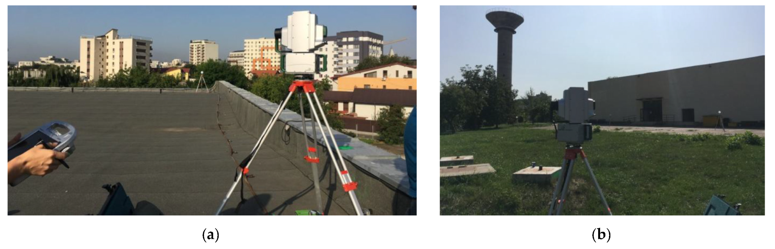
With regards to the quality assessment of the UAV obtained point clouds and meshes, the results of both types of GCPs-ChPs distributions were compared with the reference data that were obtained by TLS technology while using the “Distance-Cloud/Mesh Dist” function implemented in CloudCompare software being calculated as the Hausdorff distances between each point and the corresponding triangle surface. For the comparisons of the mesh surfaces, a point cloud was generated for the mesh to be compared by sampling each surface by one-million points.
Table 4 summarizes the standard deviation of the distances calculated between each point of the point cloud and each sampled point on the meshes automatically generated after the BBA process using four GCPs, 20 GCPs, and 150 GCPs, and the reference TLS mesh.
It is noticeable to mention that before computing the standard deviation the point cloud and the sampled mesh were manually filtered based on the histograms of the calculated distances removing outliers. The errors are divided by half when using 20 GCPs for both scenarios, systematic and stratified random, as highlighted by
Table 4. For the 150 GCPs case, the standard deviation is decreasing in the range of millimetres for the stratified random distribution and for the systematic distribution in the range of centimetres.
5. Discussion
For this study, different tests were performed for determining the suitable number and the spatial distribution of GCPs that are needed for the indirect georeferencing process of UAS images with the minimum impact on the accuracy of the final products, such as point clouds and mesh surfaces. One nadiral flight has been performed at 28 m height, over an area of about 1 ha while using a low cost UAS. The UAS image processing has been performed using the 3DF Zephyr Pro software, with the accuracy assessment of the indirect georeferencing process relying on computing the RMSE based on ChPs. Moreover, the accuracy of point clouds and mesh surfaces automatically generated based on UAS images was tested while using the Hausdorff distances [
34,
35] between each individual point and sampled points on each triangle surface, respectively, and the reference surface that is represented by a TLS mesh surface.
The research highlights that when using a systematic or a stratified random distribution of GCPs, the errors decrease significantly in the case of 20 GCPs with respect to the errors that were obtained for the eight GCPs scenario. The total RMSE decreases with only 2 cm in the case of 50 GCPs with respect to the RMSE obtained for 20 GCPs, reaching half of the error when using a very large number of GCPs (the maximum considered for this study), i.e., 4.2 cm for the systematic distribution and 4.1 cm for the stratified random distribution. The planimetric errors are slightly different in the range of 1 cm when using 20 GCPs and 150 GCPs, respectively. The stratified random distribution of GCPs and ChPs gave the best results, with the total errors being smaller at the decimetre level for the eight GCPs scenario, centimetre level for the 20, 25, and 50 GCPs, and millimetre level for the rest of scenarios.
The results are in accordance with the findings of Rangel et al. [
22], where 18 to 20 GCPs with uniform distribution on the image block is the optimum number since introducing more GCPs there is an insensitive improvement inaccuracy, even if the accuracy assessment was made for DSM and orthophotos of an open pit mine of 270 ha. The magnitudes of the RMSEz that were found in this research when using 20 GCPs in both systematic and stratified random distribution are almost the same as those found by Tonkin et al. [
20], which evaluated the vertical accuracy of DSMs with 530 ChPs with known heights.
For a better data comprehension, three control areas (
Figure 16) have been specifically selected, two inside the surface covered by the GCPs and ChPs locations (Control Area 1 and 2) representing a parking lot and the building roof, respectively, and one outside the surface that covers the parking lot situated on the right side of the building and a car access (Control Area 3). The particularity of these surfaces is that they are man-made structures with a low degree of roughness.
For the point clouds and sampled meshes that correspond to the first two control areas, the median absolute deviation (stdDevMAD), has been calculated to evaluate the accuracy for both distributions: systematic (
Table 5) and stratified random (
Table 6) while using OPALS software [
36,
37], because gross matching errors can lead to very big errors and they should not be considered in the computation of the standard deviation.
According to [
36], the median absolute deviation (stdDevMAD) is a robust standard deviation estimator computed from the median of absolute deviations from the median of all values (Equation (1)).
Being a robust statistic, the data quantification is more resilient due to the fact that large deviations as outliers do not have greater influence on the final result.
As highlighted by
Table 5 and
Table 6, the errors are approximately five times smaller when using 20 GCPs for both scenarios, systematic and stratified random. For the 150 GCPs case, the median absolute deviation is decreasing in the range of millimetres for the systematic distribution and for the stratified random distribution in range of centimetres only for Control Area 1.
An influential factor of the statistical variables results is also represented by the position of the control surfaces with respect to the area that is covered by GCPs-ChPs. Therefore, in the case of the systematic distribution, for the Control area 2 located at the border of the GCPs-ChPs area, the errors are almost five times smaller for the 20 GCPs scenario with respect to four GCPs, for point clouds and sampled meshes, while for the control area 1 located in the middle of the area the errors are even seven times smaller. For the stratified random distribution, the errors are almost five times smaller for 20 GCPs scenario with respect to four GCPs, for both control areas, but, even so, they are smaller or almost equal for the control area 1 with respect to control area 2 in most cases.
A decreasing tendency of the median absolute deviation (stdDevMAD) for all cases is visible and, regarding the 150 GCPs scenario, the differences are in the range of millimetres when compared with the 20 GCPs scenario also expressed for the residuals of 150 ChPs calculated in the Results section.
The errors corresponding to each point of the point cloud and each sampled point belonging to mesh surfaces obtained for the four GCPs, 20 GCPs, and 150 GCPs scenarios in the case of control areas 1 and 2 after the comparison with the TLS mesh, can be visualized in
Appendix A for both distribution. Comparing the point clouds and sampled meshes on control area 3 (
Figure 16) with the reference surface will give extra information regarding the error’s propagation. Therefore,
Table 7 lists the median absolute deviation (stdDevMAD) for the point clouds and sampled meshes that were obtained by UAS image processing using four GCPs in the BBA process, 20 GCPs and 150 GCPs, respectively. In the case of the systematic distribution, it can be noticed that the errors found in this area are of the same magnitude as those encountered in control areas 1 and 2 when only using four GCPs, decreasing to the decimetre level when using the suitable number, but still being two times larger than those encountered in the GCPs area. It is concluded when globally investigating the errors calculated for this area by comparing the median absolute deviation with the total RMSE that they are two times larger than in the GCPs area when using the suitable and the maximum number of GCPs.
From all of the computed scenarios, in the case of both distributions, we found that the suitable number of GCPs to be used in the BBA process without any effect on the accuracy of the final products is 20 GCPs. Moreover, the total RMSE was smaller than in the case of systematic distribution when using the stratified random distribution for the spatial location of GCPs and ChPs.
6. Conclusions
For the UAS reconstruction project, placing and measuring of GCPs can be very difficult and even impossible in some situations, so knowing the suitable number and the spatial distribution of these points is of primary interest for researchers and practitioners.
This article presented a series of tests to determine the most suitable number and the spatial distribution of GCPs needed to georeference a block of nadiral UAS images acquired with a low-cost platform, i.e., DJI Phantom 3 Standard over an urban area. The images are of high resolution having a GSD of 1.1 cm and they were taken in a cross-strip flight line configuration with high overlaps (80%/60%), with their processing being performed by bundle block adjustment with self-calibration.
The total RMSE calculated for the 150 ChPs improved with more than 50% when using 20 GCPs with respect to the four and eight GCPs scenarios and up to 80% in the case of 150 GCPs.
The metric evaluation of automatically generated point clouds and mesh surfaces was completed by comparing the points and the sampled triangles with a reference mesh, namely a TLS mesh computing the median absolute deviation (stdDevMAD) that was implemented into OPALS software, concluding that the errors outside the GCPs area are two times larger than those that are encountered in the GCPs area when using 20 GCPs or a higher number. Regarding the two control areas situated inside the GCPs and ChPs boundary, the errors are almost five times smaller for the 20 GCPs scenario with respect to four GCPs, in the case of both studied distributions. A decreasing tendency of the median absolute deviation (stdDevMAD) is visible for all cases and, regarding the 150 GCPs scenario, the differences are in the range of millimetres compared with 20 GCPs scenario also expressed for the total RMSE calculated for ChPs.
Even if there is a slightly difference between the errors that were obtained for stratified random distribution with respect to systematic distribution, in most cases they are smaller, concluding that the stratified random distribution can be used for placing the GCPs over the study area.
It can be concluded that, in order to obtain high accuracy of the final products, the following guidelines can be considered:
- -
control points in the corners are essential, but should be placed not too far out in the corners of the area of interest;
- -
eight GCPs are better than four GCPs, which is to be expected. However, placing them along the border of the block is not optimal, and interior control points are improving the accuracy significantly;
- -
a stratified random placement of control points offers a similar accuracy and an even better one than a systematic placement;
- -
an increase in the number of control points leads to improved accuracy, which is to be expected. The accuracy converges to two GSD in planimetry and three GSD in elevation;
- -
up to 20 control points the accuracy improves strongly, but for higher number of control points the improvements are only marginal. Placing 20 GCPs over a surface of approximately 4000 m2 an accuracy of 3 GSD in planimetry and 7 GSD in elevation was obtained. Keeping in mind the characteristics of the study area and the flight design, the suitable number of GCPs needed for obtaining accurate results may be specific for the presented study; and,
- -
extrapolating beyond the area enclosed by control points it leads to lower accuracy, also if a very high number of control points is used.
The results demonstrated a clear overview of the number and distribution of GCPs needed for the indirect georeferencing process with minimum influence on the final results. Future research will concentrate on a larger area, with more buildings, by flying at different flight heights.


