Abstract
Dry forests in Sub-Saharan Africa are of critical importance for the livelihood of the local population given their strong dependence on forest products. Yet these forests are threatened due to rapid population growth and predicted changes in rainfall patterns. As such, large-scale woody cover monitoring of tropical dry forests is urgently required. Although promising, remote sensing-based estimation of woody cover in tropical dry forest ecosystems is challenging due to the heterogeneous woody and herbaceous vegetation structure and the large intra-annual variability in the vegetation due to the seasonal rainfall. To test the capability of Sentinel-2 satellite imagery for producing accurate woody cover estimations, two contrasting study sites in Ethiopia and Tanzania were used. The estimation accuracy of a linear regression model using the Normalised Difference Vegetation Index (NDVI), a Partial Least Squares Regression (PLSR), and a Random Forest regression model using both single-date and multi-temporal Sentinel-2 images were compared. Additionally, the robustness and site transferability of these methods were tested. Overall, the multi-temporal PLSR model achieved the most accurate and transferable estimations (R2 = 0.70, RMSE = 4.12%). This model was then used to monitor the potential increase in woody coverage within several reforestation projects in the Degua Tembien district. In six of these projects, a significant increase in woody cover could be measured since the start of the project, which could be linked to their initial vegetation, location and shape. It can be concluded that a PLSR model combined with Sentinel-2 satellite imagery is capable of monitoring woody cover in these tropical dry forest regions, which can be used in support of reforestation efforts.
1. Introduction
In Sub-Saharan Africa, forests are crucial for the local population as they provide a range of ecosystem services such as the supply of firewood, food, and pharmaceuticals, maintenance of biodiversity, and management of water and carbon cycles in the soil [1,2]. An estimated 65% of the population is dependent on these forests for their livelihood [3]. Yet, rapid population growth increasing the need for forest products and expansion of agricultural areas leads to high deforestation rates across the whole of Sub-Saharan Africa. Moreover, predicted changes in rainfall patterns caused by climate change are expected to affect the dry woodlands and forests [4]. Within this context, there is a growing focus on more sustainable forest management and reforestation projects in tropical forest areas, although dry forests and savannas are still under-represented [1,5].
In order to assess whether these projects achieve their goal of expanding the forested area and improving its state, the development of forest monitoring tools is crucial. Typically, canopy structural parameters are measured in situ as indicators of forest stand development and they are needed to assess primary productivity, water cycles, and carbon stocks [6,7]. One particularly important structural measure is woody cover. It is defined by Gonsamo et al. [6] as “the sum of the vertical projection areas of the tree crowns divided by the horizontal area on which the trees are growing”. Woody cover is a proxy for the spatial heterogeneity and fragmentation of an area, and can be related directly to species competition and diversity, hence why it is one of the most used structural parameters [6,8,9].
Monitoring tropical dry forest vegetation using in situ measures of woody cover is however cost and labour intensive. Achieving large-scale or repeated assessments is thus challenging or even impossible, particularly over areas with limited or restricted access. Optical remote sensing techniques, mainly satellite-based, have proven to be a valuable alternative because of their wide spatial coverage, high revisit frequency and cost effectiveness [10,11,12,13]. Several studies have already explored a range of methods (such as linear, Partial Least Squares (PLSR) and Random Forest regressions) to extract woody cover from satellite imagery [12,14,15,16,17].
Although these methods have shown to robustly estimate woody cover in several forest types using optical remote sensing data [12,14,15,16,17,18], the monitoring of woody cover over tropical dry forest ecosystems remains difficult due to four important reasons. First, as these forests are relatively open, the presence of heterogeneous tree-grass structures within the system makes it difficult to distinguish between woody and herbaceous vegetation [19]. Depending on the density of the vegetation, soil background reflectance can also interfere with the prediction of the vegetation condition [20]. Second, the mixture of senescent and green vegetation throughout most of the year could limit reliable vegetation monitoring with processing methods used in other forest types [21]. As senescent vegetation has a lower chlorophyll content, it has a smaller red-to-near infrared (NIR) contrast, hampering the separation of its spectrum from the soil background [22,23]. Third, as the vegetation in these systems is highly dependent on rainfall, the vegetation coverage of tropical dry forests shows a high inter- and intra-annual variability. This causes the spectral reflectance patterns of the forest areas to vary according to water availability throughout the year, implying that single date satellite imagery is not capable of capturing these vegetation dynamics [24]. Fourth, there is a lack of model transferability between similar sites due to the different environmental conditions and spatial scales of these study sites [25]. Predictive models are often built disregarding the size and location of the study area, presuming that ecological processes are not scale-dependent, and they show the same temporal patterns in different circumstances. However, this assumption is often violated in reality [26]. The high spatial and temporal variability in the vegetation coverage of tropical dry forest systems thus demand innovative techniques to guarantee the site transferability of established relationships between in situ collected data and remote sensing data. New tools that allow the monitoring of continuous changes throughout the year should also be developed [11,17].
The launch of the Sentinel-2 constellation of the European Space Agency (ESA) in 2015 provides optical data with relatively high spatial resolution (10, 20 or 60 m) and temporal resolution (up to five days), which may offer a solution to these challenges. The combination of high spatial and temporal resolution optical data may allow to capture the large spatial variability in the vegetation density of tropical dry forests. This high temporal resolution also enables the use of a multi-temporal approach instead of single-date satellite imagery [17,27]. Despite the promising data characteristics of the Sentinel-2 satellites, the woody cover retrieval methods mentioned before have mainly been applied to other satellite data such as Landsat-8 or MODIS, which have a different spectral, temporal, and spatial resolution. Moreover, most studies focus on diverse forest ecosystems globally. The objectives of this study are thus to (i) explore the capabilities of Sentinel-2 satellite data for producing accurate woody cover estimations in tropical dry forest ecosystems, (ii) compare the influence of single-date versus multi-temporal input data, (iii) test the transferability of multiple woody cover retrieval methods across two different tropical dry forest environments, and (iv) use these methods to assess the impact of reforestation projects within this ecosystem.
2. Materials and Methods
2.1. Study Site
This research focusses on two contrasting study sites, situated in the Degua Tembien district in Ethiopia and the Monduli district in Tanzania (Figure 1a). In these districts, BOS+, a Belgian environmental and developmental organisation, facilitates small-scale programs to improve sustainable community-based forest management [28]. In Ethiopia, both governmental and non-governmental organisations are promoting area closure via the rehabilitation of degraded pastureland in so-called exclosures in order to increase the soil fertility and stimulate vegetation growth [29]. In Tanzania, projects focussing on community-based forest management and agroforestry are being implemented [30].
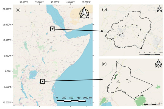
Figure 1.
(a) Map showing the study sites across East Africa; (b) Location of sampling plots in the Degua Tembien district, Ethiopia; (c) Location of sampling plots in the Monduli district, Tanzania.
The Degua Tembien district is located in the east of the Tigray Region, which is the northernmost region of Ethiopia (13° 28’ N–13° 48’ N and 39° 0’ E–39° 25’ E; Figure 1b). It has a total area of 1110 km2 and its capital city is Hagere Selam (2650 m a.s.l.) [31,32]. The average annual rainfall in the Degua Tembien district ranges from 712 to 794 mm and approximately 80% of this amount falls in the main rainy season from July to October. The dry season spans from November until February and this is followed by a pre-rainy season with scarce rainfall from March until June [33,34]. The vegetation in the Degua Tembien district can be divided in two distinct types. Firstly, the exclosures are degraded areas that are excluded from human and animal interference. They are characterised by an herbaceous layer that is green only during the rainy season and some small shrubs and trees that do not grow to their full potential due to the less than optimal site conditions [32]. Other forested areas in the Tigray region can be found in the neighbourhood of churches, since these are often enclosed within a ring of forest. This tradition of church forests has succeeded in protecting thousands of small forests over the whole of Ethiopia during the last millennium. Hence, they are preserved fragments of the original Afromontane dry forest that used to grow extensively in the Ethiopian highlands [35,36].
The Monduli district is located in the Arusha region, in the north of Tanzania. The study area includes two neighbouring villages, Selela and Mungere (3° 7’ S–3° 23’ S and 35° 51’ E–36° 10’ E, 1000–1500 m a.s.l.), and covers 450 km2 [37] (Figure 1c). The average annual rainfall in the Monduli district ranges from 200 to 600 mm with a pre-rainy season with scarce rainfall in November until February and a rainy season from March until May. The dry season spans from June until October [38]. The vegetation in the Monduli district can also be divided into two distinct types. The Serengeti volcanic grassland ecoregion primarily consists of open savannahs, while the East African montane forest ecoregion is characterised mainly by closed forests with springs [39].
2.2. In-Situ Data Collection
In order to validate the woody cover retrieval methods, in situ data were collected in both Ethiopia and Tanzania from August until October 2018. In Ethiopia and Tanzania, respectively, 39 and 40 circular plots of 1 ha were sampled over a gradient of increasing woody cover. In the Degua Tembien district, 35 plots were situated in six exclosures having low to medium woody cover (less than 30%), and four plots were located in four church forests with higher woody cover (above 30%; Figure 1b). In the Monduli district, the plots were spread between the grasslands and forest areas, with 28 plots sampled in grasslands with a low woody cover and 12 plots in the more dense forest areas (Figure 1c). The area of 1 ha coincides with approximately 16 Sentinel-2 pixels having a resolution of 20 m. This facilitates a robust comparison between field referenced data and the satellite imagery.
Each of the plots included three subplots of 400 m2. Their location relative to the plot centre was defined using a random distance and angle, with the requirements that (i) each subplot was in a different third of the plot, and (ii) the edges were located at least 10 m from each other and from the border of the plot. In every subplot, each tree or woody shrub with a stump diameter of at least 3 cm was counted as mature, while the others were considered saplings. For each mature tree, the crown diameters (i.e., the longest diameter and the diameter perpendicular to the first one) and the species were noted. The crown areas of all woody plants were then added per subplot, averaged over the three subplots and extrapolated to an area of 1 ha to produce single woody cover measurements per plot.
2.3. Remotely Sensed Data Pre-Processing
Sentinel-2 satellite imagery with processing level 1C was acquired via the Copernicus Open Access Hub [40]. For each month from November 2017 to October 2018, the image with the lowest percentage cloud cover over the two study areas was downloaded (with a maximum cloud cover of 16% for the whole image). The Multispectral Instrument on board of the Sentinel-2 satellites samples 13 bands in the visible, NIR, and shortwave-infrared (SWIR) part of the electromagnetic spectrum. These include three red edge bands (698 to 793 mm) that are specifically meant for monitoring changes in vegetation [41]. For all these images, the bands 2, 3, 4, 5, 6, 7, 8a, 11 and 12 (blue, green, red, NIR and SWIR bands) were processed to level 2A products with a resolution of 20 x 20 m using the Sen2Cor tool. This tool performs an atmospheric, terrain and cirrus correction to the Top-Of-Atmosphere Level 1C images, creating a Bottom-Of-Atmosphere image and a Scene Classification Layer [42]. Afterwards, pixels containing clouds or low-quality data were masked using the Scene Classification Layer [43].
2.4. Woody Cover Estimation
Three woody cover estimation methods were compared. First, vegetation indices such as the Normalised Difference Vegetation Index (NDVI; Rouse et al. [44]) are popular for extracting vegetation characteristics from remote sensing imagery. Their ability to estimate woody cover when included in a linear regression has been explored in a range of forest ecosystems [12,17]. Second, PLSR is a linear regression method that reduces the large number of variables to a few non-correlated linear components by optimising the covariance [14,45]. Third, Random Forest regressions are non-linear regression methods that belong to the Classification and Regression Tree methods. Each decision tree is constructed by bootstrap sampling, and from these trees a final classification is determined [15,16,18,46].
Firstly, for the linear regression, NDVI values were calculated for each monthly image and all pixel values per plot were then averaged, resulting in one NDVI value per plot per month. A linear regression between the plot-based NDVI values and the in situ collected woody cover data was then fitted to evaluate the potential of the NDVI to derive woody cover gradients. To assess temporal effects on the estimation performance, the regression was fitted both per month and using all 12 NDVI values between November 2017 and October 2018 at once. A principal components’ analysis (PCA) was performed on the 12 monthly NDVI values to remove possible multicollinearity. Secondly, PLSR was evaluated using spectral characteristics as predictor variables and the in situ collected woody cover values as response values. Different combinations of spectral and temporal characteristics were tested (Table 1). The first two models include single-date predictor variables, with the first model including only the Sentinel-2 bands (with all pixel values averaged per plot) for each month. The second model also included the monthly NDVI value, since vegetation indices and especially NDVI values have previously shown to be good predictor variables of woody cover [16,47,48]. Therefore, a multi-temporal third model only including the 12 monthly NDVI values was added as well. As PLSR models are capable of handling correlated predictors, no PCA was performed on the predictor variables. Lastly, for the Random Forest regression the same combinations of predictor variables were used as in the PLSR models (Table 1), and the in situ collected woody cover data were used as response variables. To account for the multicollinearity between the nine Sentinel-2 bands and the monthly NDVI values, PCA was performed on each set of predictor variables.

Table 1.
Predictor variables used for the Partial Least Squares Regression (PLSR) and the Random Forest regression for Ethiopia and Tanzania separately.
The spatial transferability of the methods was evaluated under three different scenarios. In the first scenario, the three methods were trained and tested using data from each study site separately. This is considered to be the baseline evaluation. For the Degua Tembien district in Ethiopia, May and August 2018 were not included in this baseline scenario since some plots were covered by clouds. Similarly, for the same reason, November 2017 and April and June 2018 were left out for the Monduli district in Tanzania. In the second scenario, the three methods were trained with data from one study site (Ethiopia or Tanzania) and tested using the other site. Because of the difference in seasonality between the Degua Tembien district in Ethiopia and the Monduli district in Tanzania, it was not possible to compare identical months between the two sites. Instead, the three months with the lowest greenness (from here on called ‘dry month 1, 2 and 3’) and the greenest month (from here on called ‘rainy month)’ were listed for each site (Table 2), and the corresponding months were then used for testing the three methods. The response spaces between the NDVI and the cellulose absorption index (CAI; Figure A1, Figure A2, and Figure A3) for both Ethiopia and Tanzania were used to determine which months were included for both study sites. For Ethiopia, the pre-rainy season months from April until June turned out to contain the driest vegetation, while for Tanzania August until October were found to have the lowest greenness. The clouded plots of May 2018 for Ethiopia were replaced by the average reflectance value of the other plots within the same exclosure. For the linear regression models, each month was first separately put into a simple linear regression and then all four months were combined in an all-year multiple linear regression. For the PLSR and the Random Forest regression, the same three models were compared: one including only the Sentinel-2 bands per month, one including the bands and NDVI per month and one including the four NDVI values of the different months combined. Lastly, the third scenario trained and tested the three methods with data from both sites combined. The months listed in Table 2 were also used in this scenario. PCA was performed on all the predictor variables of the linear and Random Forest regression models to remove the multicollinearity. A complete overview of the different methods, input data and scenarios is given in Table 3.
Table 2.
Included months in the integrated models.
Table 3.
Overview of the different retrieval methods, input data and scenarios. Each of the methods is applied on all three scenarios using both types of RS input data.
When the same data were used to train and test the models, i.e., in the first and the third scenario, the data were split into 2/3 training data and 1/3 test data. Because Moran’s I indicated spatial autocorrelation between the plots, clusters of data (for example all plots located within the same exclosure) were set aside for the training and test datasets [49]. In the second scenario, the training data came from the first study site, while the test data belonged to the other site. Ten-fold cross validation was performed on the training data to avoid overfitting of the models and the woody cover of the test dataset was determined using the final models. Both the coefficient of determination (R2) and the root mean square error (RMSE) between the estimated and the in situ measured woody cover of the test dataset were calculated using Equations (1) and (2), respectively [50].
In these equations, Ŷ is the value of Y estimated using the regression model and n is the number of predictions.
2.5. Monitoring Reforestation Efforts
The development of forest monitoring tools is essential to assess whether reforestation projects achieve their goal of increasing the woody canopy cover and, if this is not the case, to timely redirect management. To illustrate the potential of Sentinel-2 data for woody cover monitoring, the reforestation efforts of the Ethiopian organisations WeForest Ethiopia, Trees for Farmers Ethiopia and Ethiotrees in cooperation with BOS+ in 17 exclosures within the Degua Tembien district were evaluated [30]. Here, woody cover was compared between 2017, which is the starting year of the projects, and 2019. For comparison with non-managed forest areas, 25 church forests located in the Degua Tembien district were also included in this case study [51]. One Sentinel-2 image for each of the three driest months and the wettest month for both 2017 and 2019 was pre-processed. For each of the exclosures and the surrounding church forests, the average NDVI was calculated per month. The best scoring retrieval model from the combined models (Scenario 3) was then used to predict the woody cover values in 2017 and 2019. These predictions were subsequently compared using a one-sided paired t-test. This test had a null hypothesis that there was no significant difference in woody cover between 2017 and 2019, and an alternative hypothesis that the woody cover in 2019 was significantly higher than was the case in 2017.
In order to gain understanding in spatial variability of the woody cover increase between 2017 and 2019, the predicted woody cover change was linked to different landscape characteristics using Spearman’s rank correlation coefficient. Firstly, the predicted woody cover for 2017, 2018 and 2019 were calculated for the whole study area and averaged over these three years using a moving window with a window size of nine pixels to increase the robustness of the map. A second map was build calculating the standard deviation of the three yearly woody cover maps using the same moving window approach. Thirdly, a map giving the distance to the four biggest villages in the district was created based on Zenebe et al. [52]. A fourth map including the elevation of the district was derived from Shuttle Radar Topography Mission (SRTM) Void Filled data provided by USGS [53]. The fifth map included the slope of the area, which was based on the elevation map. Finally, the area to perimeter ratio of each exclosure was used to characterise its shape.
3. Results
3.1. Training and Testing Retrieval Methods with Data from the Same Study Site (Scenario 1)
In order to test the ability of the different methods (linear regression, PLSR and Random Forest regression) to quantify the woody cover using Sentinel-2 satellite imagery at each site individually, they were first trained and tested with data from the same site only. For Ethiopia, the best results of the linear regression (R2 ≥ 0.95, RMSE < 5.40%) were reached in March and April 2018 (which are both pre-rainy season months) (Table 4). The all-year-regression, integrating all months from November 2017 until October 2018, achieved similar R2 and RMSE values compared to the single-date models. For Tanzania, the months December 2017 and September and October 2018 (which are pre-rainy and dry season months) achieved the best results (R2 ≥ 0.67, RMSE ≤ 7.60%), while the all-year-regression achieved moderate results (R2 = 0.69, RMSE = 9.55%). The PLSR and the Random Forest regression were run using three different combinations of predictor variables, one including only the monthly Sentinel-2 bands, one including both the monthly NDVI value and Sentinel-2 bands and one including the NDVI values of the whole year (Table 5 and Table 6). For both the PLSR and the Random Forest regression models, the best scoring months shifted and achieved better results when NDVI was added as an extra predictor variable to the Sentinel-2 bands. The all-year NDVI models achieved estimations with a similar a/.ccuracy to the individual month models, which was in contrast with the linear regression. For Ethiopia, the PLSR achieved overall better results (R2 ≥ 0.88, RMSE < 5.45%) compared to the Random Forest regression models, while for Tanzania, the Random Forest regression models resulted in similar R2 (≥ 0.65) but lower RMSE values (≤ 6.60%) than the PLSR models. When putting the three methods alongside each other, the multi-temporal models always achieved among the best results, except for the linear regression of Tanzania.
Table 4.
Coefficient of determination (R2) and root mean square error (RMSE) of the linear regression models for Ethiopia and Tanzania separately (Scenario 1). ‘-‘ means some plots were covered by clouds so R2 and RMSE could not be calculated. In the all-year-regression in Ethiopia, May and August 2018 were left out, while in Tanzania, November 2017 and April and June 2018 were left out. The three best performing models for each study site are marked in bold.
Table 5.
R2 and RMSE of the PLSR models for Ethiopia and Tanzania separately (Scenario 1). ‘-‘ means some plots were covered by clouds so R2 and RMSE could not be calculated. In the all-year NDVI-regression in Ethiopia, May and August 2018 were left out, while in Tanzania, November 2017 and April and June 2018 were left out. The three best performing models for each study site are marked in bold.
Table 6.
R2 and RMSE of the Random Forest regression models for Ethiopia and Tanzania separately (Scenario 1). ‘-‘ means some plots were covered by clouds, so R2 and RMSE could not be calculated. In the all-year NDVI-regression in Ethiopia, May and August 2018 were left out, while in Tanzania, November 2017 and April and June 2018 were left out. The three best performing models for each study site are marked in bold.
3.2. Training Retrieval Methods with Data from One Site and Testing It Using the Other Site (Scenario 2)
In order to compare the spatial transferability of the different retrieval methods, they were trained using data from one study site and then tested using the other site. Table 7 lists the results of the all-year NDVI regressions for all three methods, while the complete results of the linear, PLS and Random Forest regression models are given in the Appendix A (Table A1, Table A2, and Table A3). For all three methods, training the model on the data from Ethiopia and testing it on Tanzania produced higher R2 values than the other way around (R2 ≥ 0.80 compared to R2 ≥ 0.63 respectively). However, the RMSE values of the Ethiopia to Tanzania models (≥ 9.00%) were also higher than those of the Tanzania to Ethiopia models (≤ 8.10%). In both cases, the linear and PLS regression models achieved more accurate estimations (R2 up to 0.06 higher and RMSE up to 1.50% lower) than the Random Forest regression models.
Table 7.
R2 and RMSE of the three all-year NDVI regression methods for the integrated models including Ethiopia and Tanzania. E → T indicates that training data are taken from Ethiopia and tested on Tanzania, while T → E indicates training data from Tanzania tested on Ethiopia (both Scenario 2). E + T indicates that the models are built on the combined data from Ethiopia and Tanzania (Scenario 3). The best performing model per scenario is marked in bold.
3.3. Training and Testing Retrieval Methods with Data Drawn from Both Sites (Scenario 3)
As it was expected that training these methods with remotely sensed data from a single site would not suffice to quantify woody cover with great accuracy [25], they were also trained and tested with the data combined from both sites in Ethiopia and Tanzania. The results of the all-year NDVI regressions for the three methods are listed in Table 7, while the complete results are given in the Appendix A (Table A4 and Table A5). For all three methods, combining the two study areas resulted in lower RMSE values than the baseline models from the first scenario with RMSE < 4.70%, although the R2 values were also lower (≤ 0.70). The PLSR model achieved the best results out of the three methods with R2 = 0.70 and RMSE = 4.12%.
3.4. Monitoring Reforestation Efforts
When the two study areas were combined in the third scenario, the all-year PLSR model produced woody cover estimations with an R2 of 0.70 and an RMSE of 4.12%. Therefore, this model was used to predict the woody cover values of the exclosures and church forests in 2017, 2018 and 2019, their mean values over this time period, and their temporal change (Figure 2 and Table A6). The one-sided paired t-test showed that, for six out of 17 exclosures, the null hypothesis was rejected at a significance level of 0.05 in favour of the alternative hypothesis, i.e., that the woody cover in 2019 was significantly larger than in 2017. For the other 11 exclosures and the church forests, the null hypothesis could not be rejected as, in these forest areas, the woody cover values of 2019 were not significantly larger than those of 2017.
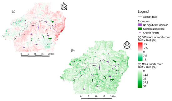
Figure 2.
(a) Map of the difference in predicted woody cover between 2017 and 2019; (b) Map of the mean woody cover between 2017 and 2019, together with the location of the 17 exclosures and 25 church forests included in the analysis.
To gain insight into the factors that may promote woody cover increase, the potential woody cover increase and relevant environmental characteristics were correlated (Figure 3). The increase in woody cover within the exclosures between 2017 and 2019 is correlated to a higher mean woody cover, lower elevation level, larger distance from villages, shallower slope, and larger area to perimeter ratio of the exclosures (Spearman’s rank correlation coefficients higher than 0.20). The standard deviation of the woody cover over three years was strongly correlated with the mean woody cover over this same time period, while its correlations with other variables were below 0.20. All maps of the relevant environmental characteristics are added in the Appendix A (Figure A4 up to Figure A7).
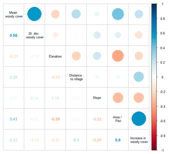
Figure 3.
Correlation plot of the characteristics of the 17 exclosures in the Degua Tembien district.
4. Discussion
4.1. Method Performance Comparison
The RMSE values achieved by the best performing models in this research range between 4.70% and 6.60% when the same area is included in training and testing of the models. The woody coverage measured in the field reached up to 53% for Ethiopia and up to 75% for Tanzania. These RMSE values thus indicate that the best models are not only capable of categorising a certain area into low or high woody cover, but also of estimating the actual woody cover with a decent accuracy.
As the NDVI is designed to enhance spectral features sensitive to vegetation greenness while reducing background disturbance [54], adding this variable to the predictor variables of the regression models was expected to improve the estimation performance. This hypothesis was confirmed by our results: including both the NDVI and the Sentinel-2 bands as predictor variables in the models resulted in better estimations for both study areas than when only the Sentinel-2 bands were included. For the PLSR models, adding NDVI increased the R2 by up to 4% and decreased the RMSE by up to 2.30%, while the Random Forest regression models had an increase in R2 of up to 7% and a decrease in RMSE up to 0.80%. These results are also confirmed by further research. Wolter et al. [14] found NDVI to be one of the most important predictor variables in PLSR when estimating woody cover in boreal forests. Other studies also found Landsat bands to be less important than vegetation indices for woody cover estimation using Random Forest regression models, although these studies did take place in different forest types [48,55].
The methods built on the data from Ethiopia gave very similar R2 values: around 0.95 for the linear regression and the PLSR, but lower for the Random Forest regression method (R2 = 0.83). The models built on the data from Tanzania and those combining the two study areas also achieved higher R2 values for the linear regression (R2 of 0.78 for Tanzania and 0.68 for combined models), but much lower values for the PLS and Random Forest regression method (R2 of 0.69 for Tanzania and 0.53 for combined models). This trend was slightly different when looking at the RMSE values of the three methods. The linear regression models achieved the lowest RMSE values, followed by the PLSR models and the Random Forest regression models. The Random Forest regression models thus seem to be less capable of estimating woody cover in a tropical dry forest environment than the linear regression or PLSR models. This is contradictory to the findings of Ahmed et al. [55] that Random Forest regression models performed better than linear regression models when estimating woody coverage in coastal temperate forests. However, in general, temperate forest ecosystems have denser canopies than tropical dry forest, which can lead to saturation of the measured reflectance. Machine learning techniques are more capable of coping with this problem than simple parametric methods are [56].
4.2. Effect of a Multi-Temporal Approach
In tropical dry forest ecosystems, most woody species keep their foliage throughout the year, while the herbaceous plants get senescent almost immediately after the rainy season ends [32,57]. Therefore, it is expected that the dry season would be preferable to the rainy season to quantify woody cover using satellite data. This assumption was confirmed for the three retrieval methods, since models based on dry season predictor variables achieved more accurate estimations than those build on rainy season months. Interestingly, adding the NDVI as a predictor variable to the monthly Sentinel-2 bands shifted the best scoring months in the PLSR and Random Forest regression models to those also scoring best in the linear regression models. These are the months that show the clearest contrast between the green woody vegetation and the dry herbaceous vegetation. This shift between the two model types also highlights the importance of NDVI compared to the satellite bands when estimating woody cover. Other research carried out in areas with a distinct dry season (e.g., a Mediterranean climate or a savanna system) also emphasized the importance of the dry season for minimising herbaceous vegetation signals when measuring woody vegetation variables [58,59,60].
By comparing models, including both single-date and multi-temporal variables, it was possible to evaluate the effect of a multi-temporal approach on the woody cover estimation accuracy. For the models including data from only one study site, the single-date models performed equal to or better than the multi-temporal models for all three methods. The RMSE values of the linear regression models increased by up to 4% when going from single-date to multi-temporal input variables, while those of the PLSR and Random Forest regression models remained very similar for both model types. However, when both study areas were combined in one model, the PLSR and Random Forest regression models achieved more accurate estimations with the multi-temporal models than with the single-date ones. This improvement was small for the PLSR (RMSE decreased 0.8%) but larger for the Random forest regression (RMSE decreased 2%). This means that the larger variety in vegetation types and seasonality when combining both study areas in one model can be captured in more detailed using multi-temporal input data. The research of Tsalyuk et al. [47] found that multi-temporal PLSR models achieved better results than single-date models for predicting tree coverage in savanna systems. As their study area covered over 20 000 km2, their explored woody cover range will surely be comparable to or even larger than the one included in the combined models of this research, confirming the explanation given here. Heiskanen and Kivinen [61] also achieved improved woody cover mapping when including multi-temporal data in their linear models within a transition zone of the taiga and the tundra. As their study site was comprised of treeless heaths, deciduous woodlands and sparse evergreen forests, this also confirms the improved woody cover estimation when including multi-temporal input data in more heterogeneous ecosystems.
Using only a subset of dry and rainy months in the models, including both the Ethiopian and Tanzanian study sites, made it possible to incorporate areas with a different seasonality. An extra advantage of this approach was the higher model flexibility compared to when all twelve months were included, as it is possible that rainy and dry seasons start earlier or later than the year the model was built.
4.3. Spatial Transferability of Methods
In general, variability in space and time hinders the transferability of remote sensing models to other regions [26,62]. By comparing three different scenarios containing the two study sites in Ethiopia and Tanzania, the transferability of the linear regression model, the PLSR model and the Random Forest regression model, were assessed. For all three methods, the models which were tested on the Ethiopian plots achieved lower RMSE values (and thus more accurate estimations) than those validated on the Tanzanian plots, even if their R2 values were not higher. This is because a smaller woody cover gradient was sampled in Ethiopia, hence the average deviations of the predicted from the actual woody cover values will automatically be smaller.
The transferred models (Scenario 2) showed similar trends to the models built and tested on the same areas (Scenario 1 and 3). The models including both Sentinel-2 bands and NDVI as predictor variables also achieved better estimations than those without NDVI for both PLSR and Random Forest regression. When looking at R2, the linear regression and PLSR models gave very similar accuracies, while the Random Forest regression models performed less good when transferred to a different area. According to the RMSE values, the linear regression models achieved the best accuracy, followed by the PLSR models (RMSE increased 0.5% compared to the linear models) and the Random Forest regression models (RMSE increased 1.2% compared to the linear models). The performance of the temporal feature also varied per used method. For the linear regression, transferring the models gave the best results when single dry season imagery was used, while the transferability of the Random Forest regression increased with multi-temporal input data. The effect of multi-temporality when transferring PLSR models was less straightforward and depended on the transfer direction. All transferred models achieved lower estimation accuracies than their counterparts including both study areas for training and validation, indicating that a larger training dataset improves the model accuracy independent of the method used. This was also found to be true for temperate and tropical humid forests in previous research [25,26,62]. The achieved RMSE values ranging from 4.5% to 9% also indicate that the transferred models will result in less exact woody cover estimations than the models build and tested on one area. However, the high R2 values (0.70–0.86) suggest that a categorisation into low and high woody cover is still possible.
Models trained in a more heterogeneous landscape are expected to capture more variability in the environmental factors, and thus estimate more accurate vegetation characteristics in other sites with less environmental variation [63]. Hence, this would imply that the models trained in Tanzania and tested on Ethiopia perform better than the other way around, which is not the case. A possible explanation could be that only four of the Ethiopian plots were located in forests that were evergreen, compared to 12 plots in Tanzania. There were thus more dry plots with a more pronounced reflectance contrast between the woody and grass or shrub vegetation in the Ethiopian study site, which allows better estimation of woody cover. Woody cover retrieval methods in tropical dry forest systems thus achieve more accurate estimations when they are trained on drier areas than those they are tested on. A study of model transferability in a semi-arid savanna system also came to this conclusion [47].
When comparing the three different scenarios, the multi-temporal PLSR models were found to be superior to the multi-temporal linear regression and Random Forest regression models when estimating woody cover. However, the transferability and robustness of all three methods could still be improved. Firstly, a possible improvement could be to include the soil fraction using spectral mixture analysis, as it is relatively insensitive to the effects of different environmental factors when transferred to a similar ecosystem, in contrast to vegetation reflectance values and indices [64]. Including topographic, bioclimatic and land surface information in the predictor variables of the different models could provide predictions with higher accuracy [65]. Secondly, including a variable selection step prior to the analysis has already been shown to increase vegetation mapping accuracies in a number of studies [48,66].
4.4. Monitoring of Reforestation Efforts
The monitoring approach used in this research assumed that a model based on field measurements collected in 2018 is also qualified to predict woody cover in 2017 and 2019. This assumption is supported by Lambert et al. [67] who found their forest monitoring method capable of expressing the forest condition in the two years preceding and succeeding the moment of field measurements. According to the t-test, six out of 17 exclosures showed a significant increase in woody cover from 2017 until 2019, indicating that in some cases the reforestation efforts did positively influence the woody vegetation growth after two years. The church forests, on the other hand, did not see a significant increase in woody cover between 2017 and 2019, which was expected. These church forests are an intrinsic part of the Ethiopian Orthodox Church and there is no indication of these forests being strategically managed as natural resources for the community [36].
The strong positive correlation between the mean woody cover value and its temporal standard deviation indicates that, according to the used PLSR model, the predicted woody cover varied more in areas with a higher woody cover than in lower woody cover areas over three years. This could mean that a higher woody cover promotes its increase, therefore leading to larger differences between the years. This explanation is also backed by the positive correlation between mean woody cover and woody cover increase. Another possibility could be that our model gives more accurate predictions for lower woody cover areas, leading to less inter-annual variability. However, no clear over- or underestimation for certain woody cover ranges could be found in our analyses. Furthermore, the woody cover increase since 2017 showed a negative correlation with elevation. This was unexpected, as other research found an increase in species richness and diversity when exclosures were located on a higher elevation [68]. This increase was explained by the presence of higher precipitation and less anthropogenic disturbances at higher elevations, which are variables that would also affect the presence of woody vegetation. Therefore, it seems that the correlation between elevation and woody cover increase is indirectly led by the strong positive correlation (R2 = 0.6) between woody cover increase and the area to perimeter ratio and its strong negative correlation (R2 = 0.39) with elevation. This positive correlation with a higher area to perimeter ratio also suggests that the woody cover increase is enhanced when there are less edge effects. This would mean that more circular exclosures are more effective in increasing woody vegetation than their elongated counterparts. The positive correlation (R2 = 0.29) between shallower slopes and woody cover increase is consistent with the expectation that steeper slopes would intensify erosion and thus provide inferior conditions for plant growth. Lastly, the positive correlation between the increase in woody coverage and the increasing distance to large villages can be explained by the occurrence of illegal harvesting, i.e., people harvesting forest products from exclosures, even though they have restricted access [69]. The further these exclosures are located from villages, the less illegal grazing or logging will is likely to take place.
5. Conclusions
The first objective of this study was to explore the capabilities and limitations of Sentinel-2 satellite data for producing accurate woody cover estimations in tropical dry forest ecosystems. This ecosystem has received considerably less attention compared to temperate and boreal forest systems. Two contrasting study sites in Ethiopia and Tanzania that capture a gradient of woody cover within their vegetation were chosen as reference ecosystems. Simple linear, PLS and Random Forest regressions were compared both when a smaller and larger variation in vegetation was included in the study area. Both scenarios emphasized the importance of NDVI included in the predictor variables and the combined models showed the added value of the multi-temporal approach to manage the increased variation captured in the study area, which was the second research objective. Both the single-date, dry-month linear regression model and the multi-temporal PLSR model gave very promising results for woody cover estimation in tropical dry-forest ecosystems. The third objective was to test the transferability of these woody cover retrieval methods using the two different study sites. Building and testing a model using both study areas always resulted in better estimations than when a model was tested on a different area than it was built on, indicating that a more varied training dataset improved the estimation accuracy. Moreover, the transferability of models was also found to be higher when the training environment was drier than the testing environment. Overall, the multi-temporal PLSR model was found to be the most transferable among the three retrieval methods. Therefore, this model was used within the last research objective to assess the impact of reforestation efforts in the exclosures of the Degua Tembien district in Ethiopia. Six of the 17 exclosures showed a significant increase in woody coverage between the period 2017 and 2019, which could mostly be linked to the initial vegetation, location and shape of the exclosures.
From this research it can be concluded that a PLSR model including Sentinel-2 satellite imagery is capable of overcoming most of the complications linked to extracting vegetation characteristics in tropical dry forest ecosystems. The use of multi-temporal Sentinel-2 input data combined with NDVI values enables the distinction between both woody and herbaceous and green and senescent vegetation. Moreover, it also provides a robust and transferable model that is able to estimate woody cover with high accuracy. Therefore, this model could be used for the monitoring of future reforestation projects.
Author Contributions
All authors have read and agreed to the published version of the manuscript. conceptualization, J.V.P., W.D.K and B.S.; methodology, J.V.P.,W.D.K and B.S; software, J.V.P.; validation, J.V.P.; formal analysis, J.V.P.; investigation, J.V.P.; resources, W.D.K. and B.S.; data curation, J.V.P.; writing—original draft preparation, J.V.P.; writing—review and editing, W.D.K. and B.S.; visualization, J.V.P.; supervision, W.D.K. and B.S.; project administration, J.V.P.; funding acquisition, B.S.
Funding
The research presented in this paper is partly funded by the Belgian Science Policy Office in the framework of the STEREOIII program (project U-TURN, SR/00/339)).
Acknowledgments
The authors would like to thank BOS+ for their support with the logistics of the field work in both Ethiopia and Tanzania and Kelly Wittemans for her support with the field work in Tanzania.
Conflicts of Interest
The authors declare no conflict of interest.
Appendix A

Figure A1.
Response space between NDVI and cellulose absorption index (CAI) [11]. CAI is calculated using Sentinel-2 bands 11 and 12, and it can be used to distinguish dry vegetation because reflectance in those wavelengths is absent in soil and green vegetation. The response space between NDVI and CAI can be used to estimate the fractions of photosynthetic vegetation (PV), non-photosynthetic (NPV) and bare soil (BS) within a pixel. When the pure spectra of PV, NPV and BS are known, the reflectance spectra of mixed pixels (such as point d) will be shown inside the triangle and can be compared for fractional cover values.

Figure A2.
Location of the Ethiopian plots in the NDVI – CAI response space for every month from November 2017 until October 2018. The more the plots verge to the right corner of the triangle, the greener they are, while the upper left corner indicates that more NPV, such as dry and senescent plants, is present in the plots.

Figure A3.
Location of the Tanzanian plots in the NDVI – CAI response space for every month from November 2017 until October 2018. The more the plots verge to the right corner of the triangle, the greener they are, while the upper left corner indicates that more NPV, such as dry and senescent plants, is present in the plots.
Table A1.
R2 and RMSE of the linear regression for the integrated models including Ethiopia and Tanzania (Scenario 2). E → T indicates that training data are taken from Ethiopia and tested on Tanzania, while T → E indicates training data from Tanzania tested on Ethiopia. The best performing model for each study site is marked in bold.
| Sentinel-2 Data Included | NDVI E → T | NDVI T → E | ||
|---|---|---|---|---|
| R2 | RMSE (%) | R2 | RMSE (%) | |
| Dry month 1 | 0.81 | 10.36 | 0.74 | 5.86 |
| Dry month 2 | 0.87 | 8.32 | 0.67 | 6.98 |
| Dry month 3 | 0.87 | 13.95 | 0.56 | 14.74 |
| Rainy month | 0.37 | 18.55 | 0.13 | 11.29 |
| All-year | 0.86 | 10.15 | 0.72 | 6.96 |
Table A2.
R2 and RMSE of the PLSR for the integrated models including Ethiopia and Tanzania (Scenario 2). E → T indicates that training data are taken from Ethiopia and validated on Tanzania, while T → E indicates training data from Tanzania validated on Ethiopia. The two best performing models for each study site are marked in bold.
| PLSR Model | E → T | T → E | ||||||
|---|---|---|---|---|---|---|---|---|
| Bands | Bands + NDVI | Bands | Bands + NDVI | |||||
| R2 | RMSE (%) | R2 | RMSE (%) | R2 | RMSE (%) | R2 | RMSE (%) | |
| Dry month 1 | 0.83 | 14.70 | 0.81 | 11.68 | 0.69 | 7.15 | 0.73 | 6.25 |
| Dry month 2 | 0.88 | 10.82 | 0.85 | 9.64 | 0.56 | 7.94 | 0.59 | 7.58 |
| Dry month 3 | 0.83 | 18.94 | 0.45 | 20.85 | 0.34 | 9.71 | 0.41 | 13.00 |
| Rainy month | 0.26 | 48.04 | 0.28 | 32.23 | 0.10 | 15.79 | 0.18 | 15.06 |
| All-year NDVI | 0.86 | 9.00 | 0.63 | 7.27 | ||||
Table A3.
R2 and RMSE of the Random Forest regression for the integrated models including Ethiopia and Tanzania (Scenario 2). E → T indicates that training data are taken from Ethiopia and validated on Tanzania, while T → E indicates training data from Tanzania validated on Ethiopia. The two best performing models for each study site are marked in bold.
| Random Forest Regression Model | E → T | T → E | ||||||
|---|---|---|---|---|---|---|---|---|
| Bands | Bands + NDVI | Bands | Bands + NDVI | |||||
| R2 | RMSE (%) | R2 | RMSE (%) | R2 | RMSE (%) | R2 | RMSE (%) | |
| Dry month 1 | 0.36 | 20.41 | 0.72 | 13.65 | 0.30 | 9.56 | 0.55 | 7.71 |
| Dry month 2 | 0.38 | 18.50 | 0.74 | 13.85 | 0.42 | 10.08 | 0.44 | 12.25 |
| Dry month 3 | 0.81 | 13.19 | 0.71 | 17.91 | 0.13 | 13.57 | 0.26 | 18.46 |
| Rainy month | 0.00 | 23.14 | 0.02 | 21.74 | 0.33 | 9.75 | 0.38 | 8.98 |
| All-year NDVI | 0.80 | 10.66 | 0.67 | 8.10 | ||||
Table A4.
R2 and RMSE of the linear regression for the models combining Ethiopia and Tanzania (Scenario 3). The best performing model is marked in bold.
Table A4.
R2 and RMSE of the linear regression for the models combining Ethiopia and Tanzania (Scenario 3). The best performing model is marked in bold.
| Sentinel-2 Data Included | NDVI | |
|---|---|---|
| R2 | RMSE (%) | |
| Dry month 1 | 0.68 | 4.17 |
| Dry month 2 | 0.63 | 4.96 |
| Dry month 3 | 0.06 | 8.25 |
| Rainy month | 0.04 | 15.64 |
| All-year | 0.61 | 4.65 |
Table A5.
R2 and RMSE of the PLSR and Random Forest regression for the models combining Ethiopia and Tanzania (Scenario 3). The two best performing models for every method are marked in bold.
Table A5.
R2 and RMSE of the PLSR and Random Forest regression for the models combining Ethiopia and Tanzania (Scenario 3). The two best performing models for every method are marked in bold.
| Regression Model | PLSR | Random Forest Regression | ||||||
|---|---|---|---|---|---|---|---|---|
| Bands | Bands + NDVI | Bands | Bands + NDVI | |||||
| R2 | RMSE (%) | R2 | RMSE (%) | R2 | RMSE (%) | R2 | RMSE (%) | |
| Dry month 1 | 0.55 | 7.33 | 0.65 | 4.36 | 0.26 | 12.71 | 0.47 | 8.39 |
| Dry month 2 | 0.57 | 7.16 | 0.59 | 5.25 | 0.54 | 6.74 | 0.51 | 7.95 |
| Dry month 3 | 0.52 | 5.14 | 0.10 | 7.33 | 0.25 | 6.45 | 0.10 | 7.70 |
| Rainy month | 0.04 | 14.47 | 0.11 | 12.64 | 0.04 | 13.30 | 0.09 | 13.91 |
| All-year NDVI | 0.70 | 4.12 | 0.59 | 4.73 | ||||
Table A6.
The mean predicted woody cover values for each exclosure and the church forests for 2017 and 2019, together with the p-values of the one-sided t-test. All 25 church forests were merged for the t-test calculation for simplicity. The p-values smaller than 0.05 are shown in bold.
Table A6.
The mean predicted woody cover values for each exclosure and the church forests for 2017 and 2019, together with the p-values of the one-sided t-test. All 25 church forests were merged for the t-test calculation for simplicity. The p-values smaller than 0.05 are shown in bold.
| Name Exclosure | Mean Predicted Woody Cover in 2017 (%) | Mean Predicted Woody Cover in 2019 (%) | P-Value Of One-Sided t-Test |
|---|---|---|---|
| Adi Amik | 10.29 | 8.18 | 1.00 |
| Adi Meles | 13.38 | 15.06 | 0.00 |
| May Hibo | 21.52 | 20.42 | 1.00 |
| May Getnet | 12.12 | 13.22 | 0.00 |
| Gereb Endaboy Hailu | 18.22 | 16.48 | 1.00 |
| Daero Hidag | 19.88 | 20.66 | 0.00 |
| Afedena | 10.94 | 10.16 | 1.00 |
| Aynmbrkekin | 14.61 | 14.01 | 1.00 |
| Selam | 13.48 | 14.74 | 0.00 |
| Seret | 12.90 | 11.41 | 1.00 |
| Adi Lethsi | 17.08 | 17.45 | 0.00 |
| Meam Atali | 21.66 | 21.70 | 0.24 |
| Chelako | 22.83 | 21.05 | 1.00 |
| Gemgema | 17.97 | 14.86 | 1.00 |
| May Baati | 17.77 | 13.34 | 1.00 |
| Qatina Ruba | 9.43 | 8.93 | 1.00 |
| Taakuro | 17.81 | 19.74 | 0.00 |
| Church forests | 26.03 | 25.02 | 1.00 |

Figure A4.
Standard deviation between predicted woody cover from the period 2017 to 2019, together with the location of the 17 exclosures and 25 church forests included in the analysis.

Figure A5.
Distance from the four largest villages within the Degua Tembien district, together with the location of the 17 exclosures and 25 church forests included in the analysis.

Figure A6.
Elevation of the Degua Tembien district, together with the location of the 17 exclosures and 25 church forests included in the analysis.

Figure A7.
Slope of the Degua Tembien district, together with the location of the 17 exclosures and 25 church forests included in the analysis.
References
- FAO. Global Forest Resources Assessment 2015; FAO: Rome, Italy, 2015; ISBN 9789251092835. [Google Scholar]
- Perera, A.H.; Perterson, U.; Pastur, G.M.; Iverson, L.R. Ecosystem Services from Forest Landscapes; Springer: Cham, Switzerland, 2018; ISBN 9783319745145. [Google Scholar]
- Dieng, C.; Katerere, Y.; Kojwang, H.; Laverdière, M.; Minang, P.A.; Mulimo, P.; Mwangi, E.; Oteng-Yeboah, A.; Sedashonga, C.; Swallow, B.; et al. Making Sub-Saharan African Forests Work for People and Nature; Katerere, Y., Minang, P.A., Vanhanen, H., Eds.; IUFRO’s Special Project on World Forests, Society and Environment (WFSE); IUFRO: Vienna, Austria, 2009; ISBN 9789290592563. [Google Scholar]
- IPCC. Climate Change 2014: Impacts, Adaptation and Vulnerability; Cambridge University Press: Cambridge, UK, 2014; ISBN 9781107641655. [Google Scholar]
- Pennington, R.T.; Lehmann, C.E.R.; Rowland, L.M. Tropical savannas and dry forests. Curr. Biol. 2018, 28, R541–R545. [Google Scholar] [CrossRef] [PubMed]
- Gonsamo, A.; D’Odorico, P.; Pellikka, P. Measuring fractional forest canopy element cover and openness—Definitions and methodologies revisited. Oikos 2013, 122, 1283–1291. [Google Scholar] [CrossRef]
- Naidoo, L.; Mathieu, R.; Main, R.; Kleynhans, W.; Wessels, K.; Asner, G.; Leblon, B. Savannah woody structure modelling and mapping using multi-frequency (X-, C- and L-band) Synthetic Aperture Radar data. ISPRS J. Photogramm. Remote Sens. 2015, 105, 234–250. [Google Scholar] [CrossRef]
- Madonsela, S.; Azong, M.; Ramoelo, A.; Mutanga, O. Estimating tree species diversity in the savannah using NDVI and woody canopy cover. Int. J. Appl. Earth Obs. Geoinf. 2018, 66, 106–115. [Google Scholar] [CrossRef]
- Mathieu, R.; Naidoo, L.; Cho, M.A.; Leblon, B.; Main, R.; Wessels, K.; Asner, G.P.; Buckley, J.; Van Aardt, J.; Erasmus, B.F.N.; et al. Toward structural assessment of semi-arid African savannahs and woodlands: The potential of multitemporal polarimetric RADARSAT-2 fine beam images. Remote Sens. Environ. 2013, 138, 215–231. [Google Scholar] [CrossRef]
- Brandt, M.; Hiernaux, P.; Tagesson, T.; Verger, A.; Rasmussen, K.; Aziz, A.; Mbow, C.; Mougin, E.; Fensholt, R. Woody plant cover estimation in drylands from Earth Observation based seasonal metrics. Remote Sens. Environ. 2016, 172, 28–38. [Google Scholar] [CrossRef]
- Guerschman, P.J.; Hill, M.J.; Renzullo, L.J.; Barrett, D.J.; Marks, A.S.; Botha, E.J. Estimating fractional cover of photosynthetic vegetation, non-photosynthetic vegetation and bare soil in the Australian tropical savanna region upscaling the EO-1 Hyperion and MODIS sensors. Remote Sens. Environ. 2009, 113, 928–945. [Google Scholar] [CrossRef]
- Wu, W. Derivation of tree canopy cover by multiscale remote sensing approach. ISPRS Work. Geospat. Data Infrastruct. 2009, 142–149. [Google Scholar] [CrossRef]
- Lu, D. The potential and challenge of remote sensing-based biomass estimation. Int. J. Remote Sens. 2006, 27, 1297–1328. [Google Scholar] [CrossRef]
- Wolter, P.T.; Townsend, P.A.; Sturtevant, B.R. Estimation of forest structural parameters using 5 and 10 meter SPOT-5 satellite data. Remote Sens. Environ. 2009, 113, 2019–2036. [Google Scholar] [CrossRef]
- Gessner, U.; Machwitz, M.; Conrad, C.; Dech, S. Estimating the fractional cover of growth forms and bare surface in savannas. A multi-resolution approach based on regression tree ensembles. Remote Sens. Environ. 2013, 129, 90–102. [Google Scholar] [CrossRef]
- Ludwig, M.; Morgenthal, T.; Detsch, F.; Higginbottom, T.P.; Lezama Valdes, M.; Nauss, T.; Meyer, H. Machine learning and multi-sensor based modelling of woody vegetation in the Molopo Area, South Africa. Remote Sens. Environ. 2019, 222, 195–203. [Google Scholar] [CrossRef]
- Hill, M.J. Vegetation index suites as indicators of vegetation state in grassland and savanna: An analysis with simulated SENTINEL 2 data for a North American transect. Remote Sens. Environ. 2013, 137, 94–111. [Google Scholar] [CrossRef]
- Herrmann, S.M.; Wickhorst, A.J.; Marsh, S.E. Estimation of tree cover in an agricultural parkland of senegal using rule-based regression tree modeling. Remote Sens. 2013, 5, 4900–4918. [Google Scholar] [CrossRef]
- Hill, M.J.; Renzullo, L.J.; Guerschman, J.; Marks, A.S.; Barrett, D.J. Use of vegetation index “fingerprints” from hyperion data to characterize vegetation states within land cover/land use types in an australian tropical savanna. IEEE J. Sel. Top. Appl. Earth Obs. Remote Sens. 2013, 6, 309–319. [Google Scholar] [CrossRef]
- Ali, I.; Cawkwell, F.; Dwyer, E.; Barrett, B.; Green, S. Satellite remote sensing of grasslands: From observation to management. J. Plant Ecol. 2016, 9, 649–671. [Google Scholar] [CrossRef]
- Mougin, E.; Demarez, V.; Diawara, M.; Hiernaux, P.; Soumaguel, N.; Berg, A. Estimation of LAI, fAPAR and fCover of Sahel rangelands (Gourma, Mali). Agric. For. Meteorol. 2014, 198, 155–167. [Google Scholar] [CrossRef]
- Mayr, M.J.; Samimi, C. Comparing the dry season in-situ Leaf Area Index (LAI) derived from high-resolution RapidEye imagery with MODIS LAI in a Namibian savanna. Remote Sens. 2015, 7, 4834–4857. [Google Scholar] [CrossRef]
- Huete, A.R. A soil-adjusted vegetation index (SAVI). Remote Sens. Environ. 1988, 25, 295–309. [Google Scholar] [CrossRef]
- Kamusoko, C.; Gamba, J.; Murakami, H. Mapping woodland cover in the miombo ecosystem: A comparison of machine learning classifiers. Land 2014, 3, 524–540. [Google Scholar] [CrossRef]
- Cutler, M.E.J.; Boyd, D.S.; Foody, G.M.; Vetrivel, A. Estimating tropical forest biomass with a combination of SAR image texture and Landsat TM data: An assessment of predictions between regions. ISPRS J. Photogramm. Remote Sens. 2012, 70, 66–77. [Google Scholar] [CrossRef]
- Jin, S.; Su, Y.; Gao, S.; Hu, T.; Liu, J.; Guo, Q. The transferability of Random Forest in canopy height estimation from multi-source remote sensing data. Remote Sens. 2018, 10, 1183. [Google Scholar] [CrossRef]
- Korhonen, L.; Hadi; Packalen, P.; Rautiainen, M. Comparison of Sentinel-2 and Landsat 8 in the estimation of boreal forest canopy cover and leaf area index. Remote Sens. Environ. 2017, 195, 259–274. [Google Scholar] [CrossRef]
- BOS+. Available online: https://www.bosplus.be/nl/wat-we-doen (accessed on 16 April 2020).
- FDRE. Ethiopia’s Climate-Resilient Green Economy: Green Economy Strategy; Federal Democratic Republic of Ethiopia: Addis Ababa, Ethiopia, 2011; pp. 1–200. [Google Scholar]
- BOS+. Tanzania Programme. In Het meerjarenplan 2017-2021 van BOS+ tropen vzw. 2017; pp. 255–296. Available online: https://www.bosplus.be/l/library/download/urn:uuid:a67686d9-fbf8-4861-ab21-1bc34cd04977/beleidsplan+2017-2021_bos%2B+vlaanderen.pdf?&ext=.pdf (accessed on 16 April 2020).
- Babulo, B.; Muys, B.; Haregeweyn, N.; Descheemaeker, K.; Deckers, J.; Poesen, J.; Nyssen, J.; Mathijs, E. Cost-benefit analysis of soil and water conservation measure: The case of exclosures in northern Ethiopia. For. Policy Econ. 2012, 15, 27–36. [Google Scholar]
- Descheemaeker, K.; Muys, B.; Nyssen, J.; Poesen, J.; Raes, D.; Haile, M.; Deckers, J. Litter production and organic matter accumulation in exclosures of the Tigray highlands, Ethiopia. For. Ecol. Manag. 2006, 233, 21–35. [Google Scholar] [CrossRef]
- Babulo, B. Economic valuation and management of common-pool resources: The case of exclosures in the highlands of Tigray, Northern Ethiopia. Ph.D. Thesis, Katholieke Universiteit, Leuven, Belgium, 18 October 2007. [Google Scholar]
- Gebrehiwot, T.; van der Veen, A. Climate change vulnerability in Ethiopia: Disaggregation of Tigray Region. J. East. Afr. Stud. 2013, 7, 607–629. [Google Scholar] [CrossRef]
- Aerts, R. Church forests in Ethiopia. Front. Ecol. Environ. 2007, 5, 66–69. [Google Scholar]
- Klepeis, P.; Orlowska, I.A.; Kent, E.F.; Cardelús, C.L.; Scull, P.; Wassie Eshete, A.; Woods, C. Ethiopian church forests: A hybrid model of protection. Hum. Ecol. 2016, 44, 715–730. [Google Scholar] [CrossRef]
- Chorowicz, J. The East African rift system. J. Afr. Earth Sci. 2005, 43, 379–410. [Google Scholar] [CrossRef]
- ADF. African Development Fund (ADF) Monduli District Water Project 2003; ADF: Tunis, Tunis, 2003. [Google Scholar]
- Olson, D.M.; Dinerstein, E.; Wikramanayake, E.D.; Burgess, N.D.; Powell, G.V.N.; Underwood, E.C.; Kassem, K.R. Terrestrial ecoregions of the world: A new map of life on earth. Bioscience 2001, 51, 933–938. [Google Scholar] [CrossRef]
- ESA; Copernicus. European Commission Copernicus Open Access Hub. Available online: https://scihub.copernicus.eu/dhus/#/home (accessed on 2 January 2019).
- ESA Sentinel-2. Available online: https://sentinel.esa.int/web/sentinel/missions/sentinel-2 (accessed on 11 December 2018).
- ESA Sen2Cor. Available online: http://step.esa.int/main/third-party-plugins-2/sen2cor/ (accessed on 2 January 2019).
- ESA. Sentinel-2. Sen2Cor Configuration and User Manual. 2019. Available online: http://step.esa.int/main/third-party-plugins-2/sen2cor/sen2cor_v2-8/ (accessed on 16 April 2020).
- Rouse, J.; Haas, R.; Schell, J.; Deering, D.; Harlan, J. Monitoring the Vernal Advancement of Retrogradation of Natural Vegetation, type III; NASA/GSFC: Greenbelt, MD, USA, 1974. [Google Scholar]
- Næsset, E.; Bollandsås, O.M.; Gobakken, T. Comparing regression methods in estimation of biophysical properties of forest stands from two different inventories using laser scanner data. Remote Sens. Environ. 2005, 94, 541–553. [Google Scholar] [CrossRef]
- Breiman, L. Random forests. Mach. Learn. 2001, 45, 5–32. [Google Scholar] [CrossRef]
- Tsalyuk, M.; Kelly, M.; Getz, W.M. Improving the prediction of African savanna vegetation variables using time series of MODIS products. ISPRS J. Photogramm. Remote Sens. 2017, 131, 77–91. [Google Scholar] [CrossRef] [PubMed]
- Karlson, M.; Ostwald, M.; Reese, H.; Sanou, J.; Tankoana, B.; Mattson, E. Mapping tree canopy cover and aboveground biomass in sudano-sahelian woodlands using landsat 8 and random forest. Remote Sens. 2015, 7, 10017–10041. [Google Scholar] [CrossRef]
- MORAN, P.A.P. Notes on continuous stochastic phenomena. Biometrika 1950, 37, 17–23. [Google Scholar] [CrossRef] [PubMed]
- Anderson-Sprecher, R. Model comparisons and R2. Am. Stat. 1994, 48, 113–117. [Google Scholar]
- Aerts, R.; Lerouge, F.; November, E. Birds of forests and open woodlands in the highlands of Dogu’a Tembien. In Geo-Trekking in Ethiopia’s Tropical Mountains; Nyssen, J., Jacob, M., Frankl, A., Eds.; Springer: Berlin/Heidelberg, Germany, 2019; pp. 261–277. ISBN 978-3-030-04954-6. [Google Scholar]
- Zenebe, A.; Girma, A.; Guyassa, E.; Ashafa, T.G.; Munro, R.N.; Haile, M.; Poesen, J.; Deckers, J.; Nyssen, J. Land use and suitability for rainfed agriculture. In Geotrekking in Ethiopia’s Tropical Mountains; Nyssen, J., Jacob, M., Frankl, A., Eds.; Springer: Berlin/Heidelberg, Germany, 2019; pp. 373–386. ISBN 978-3-030-04954-6. [Google Scholar]
- USGS EarthExplorer—Home. Available online: https://earthexplorer.usgs.gov/ (accessed on 24 February 2020).
- Glenn, E.P.; Huete, A.R.; Nagler, P.L.; Nelson, S.G. Relationship between remotely-sensed vegetation indices, canopy attributes and plant physiological processes: What vegetation indices can and cannot tell us about the landscape. Sensors 2008, 8, 2136–2160. [Google Scholar] [CrossRef]
- Ahmed, O.S.; Franklin, S.E.; Wulder, M.A.; White, J.C. Characterizing stand-level forest canopy cover and height using Landsat time series, samples of airborne LiDAR, and the Random Forest algorithm. ISPRS J. Photogramm. Remote Sens. 2015, 101, 89–101. [Google Scholar] [CrossRef]
- Verrelst, J.; Camps-valls, G.; Muñoz-marí, J.; Pablo, J.; Veroustraete, F.; Clevers, J.G.P.W.; Moreno, J. Optical remote sensing and the retrieval of terrestrial vegetation bio-geophysical properties—A review. ISPRS J. Photogramm. Remote Sens. 2015, 108, 273–290. [Google Scholar] [CrossRef]
- Descheemaeker, K.; Nyssen, J.; Rossi, J.; Poesen, J.; Haile, M.; Raes, D.; Muys, B.; Moeyersons, J.; Deckers, S. Sediment deposition and pedogenesis in exclosures in the Tigray highlands, Ethiopia. Geoderma 2006, 132, 291–314. [Google Scholar] [CrossRef]
- Macedo, F.L.; Sousa, A.M.O.; Gonçalves, A.C.; José, R.; Silva, M.; Mesquita, P.A.; Rodrigues, R.A.F.; Macedo, F.L.; Sousa, A.M.O.; Gonçalves, A.C. Above-ground biomass estimation for Quercus rotundifolia using vegetation indices derived from high spatial resolution satellite images. Eur. J. Remote Sens. 2018, 51, 932–944. [Google Scholar] [CrossRef]
- Higginbottom, T.P.; Symeonakis, E.; Meyer, H.; van der Linden, S. Mapping fractional woody cover in semi-arid savannahs using multi-seasonal composites from Landsat data. ISPRS J. Photogramm. Remote Sens. 2018, 139, 88–102. [Google Scholar] [CrossRef]
- Urbazaev, M.; Thiel, C.; Mathieu, R.; Naidoo, L.; Levick, S.R.; Smit, I.P.J.; Asner, G.P.; Schmullius, C. Assessment of the mapping of fractional woody cover in southern African savannas using multi-temporal and polarimetric ALOS PALSAR L-band images. Remote Sens. Environ. 2015, 166, 138–153. [Google Scholar] [CrossRef]
- Heiskanen, J.; Kivinen, S. Assessment of multispectral, -temporal and -angular MODIS data for tree cover mapping in the tundra-taiga transition zone. Remote Sens. Environ. 2008, 112, 2367–2380. [Google Scholar] [CrossRef]
- Foody, G.M.; Boyd, D.S.; Cutler, M.E.J. Predictive relations of tropical forest biomass from Landsat TM data and their transferability between regions. Remote Sens. Environ. 2003, 85, 463–474. [Google Scholar] [CrossRef]
- Fernández-Guisuraga, J.M.; Calvo, L.; Fernández-García, V.; Marcos-Porras, E.; Taboada, Á.; Suárez-Seoane, S. Efficiency of remote sensing tools for post-fire management along a climatic gradient. For. Ecol. Manag. 2019, 433, 553–562. [Google Scholar] [CrossRef]
- Lu, D.; Batistella, M.; Moran, E.; Hetrick, S.; Alves, D.; Brondizio, E. Fractional forest cover mapping in the Brazilian Amazon with a combination of MODIS and TM images. Int. J. Remote Sens. 2011, 32, 7131–7149. [Google Scholar] [CrossRef]
- Liu, X.; Liu, H.; Qiu, S.; Wu, X.; Tian, Y.; Hao, Q. An improved estimation of regional fractional woody/herbaceous cover using combined satellite data and high-quality training samples. Remote Sens. 2017, 9, 32. [Google Scholar] [CrossRef]
- Pandit, S.; Tsuyuki, S.; Dube, T. Estimating above-ground biomass in sub-tropical buffer zone community forests, Nepal, using Sentinel 2 data. Remote Sens. 2018, 10, 601. [Google Scholar] [CrossRef]
- Lambert, J.; Drenou, C.; Denux, J.P.; Balent, G.; Cheret, V. Monitoring forest decline through remote sensing time series analysis. GIScience Remote Sens. 2013, 50, 437–457. [Google Scholar] [CrossRef]
- Woldu, G.; Solomon, N.; Hishe, H.; Gebrewahid, H.; Gebremedhin, M.A.; Birhane, E. Topographic variables to determine the diversity of woody species in the exclosure of Northern Ethiopia. Heliyon 2020, 6, 1–6. [Google Scholar] [CrossRef] [PubMed]
- Jacob, M.; Lanckriet, S.; Descheemaeker, K. Exclosures as primary option for reforestation in Dogu’a Tembien. In Geo-Trekking in Ethiopia’s Tropical Mountains; Nyssen, J., Jacob, M., Frankl, A., Eds.; Springer: Berlin/Heidelberg, Germany, 2019; pp. 251–260. ISBN 978-3-030-04954-6. [Google Scholar]
© 2020 by the authors. Licensee MDPI, Basel, Switzerland. This article is an open access article distributed under the terms and conditions of the Creative Commons Attribution (CC BY) license (http://creativecommons.org/licenses/by/4.0/).