Article

A Novel Deep Learning Method to Identify Single Tree Species in UAV-Based Hyperspectral Images

by
Gabriela Takahashi Miyoshi
1,*,
Mauro dos Santos Arruda
2,
Lucas Prado Osco
3,4,
José Marcato Junior
4,
Diogo Nunes Gonçalves
2,
Nilton Nobuhiro Imai
1,5,
Antonio Maria Garcia Tommaselli
1,5,
Eija Honkavaara
6 and
Wesley Nunes Gonçalves
2,4
1
Graduate Program in Cartographic Sciences, São Paulo State University (UNESP), Presidente Prudente 19060-900, SP, Brazil
2
Graduate Program in Computer Sciences, Faculty of Computer Science, Federal University of Mato Grosso do Sul (UFMS), Av. Costa e Silva, Campo Grande 79070-900, Brazil
3
Faculty of Engineering and Architecture and Urbanism, University of Western São Paulo (UNOESTE), R. José Bongiovani, Cidade Universitária, Presidente Prudente 19050-920, SP, Brazil
4
Faculty of Engineering, Architecture, and Urbanism and Geography, Federal University of Mato Grosso do Sul (UFMS), Av. Costa e Silva, Campo Grande 79070-900, Brazil
5
Department of Cartography, São Paulo State University (UNESP), Presidente Prudente 19060-900, SP, Brazil
6
Finnish Geospatial Research Institute, National Land Survey of Finland, Geodeetinrinne 2, 02430 Masala, Finland
*
Author to whom correspondence should be addressed.
Remote Sens. 2020, 12(8), 1294; https://doi.org/10.3390/rs12081294
Submission received: 2 April 2020 / Revised: 15 April 2020 / Accepted: 17 April 2020 / Published: 19 April 2020
(This article belongs to the Special Issue Thematic Information Extraction and Application in Forests)

Abstract

:
Deep neural networks are currently the focus of many remote sensing approaches related to forest management. Although they return satisfactory results in most tasks, some challenges related to hyperspectral data remain, like the curse of data dimensionality. In forested areas, another common problem is the highly-dense distribution of trees. In this paper, we propose a novel deep learning approach for hyperspectral imagery to identify single-tree species in highly-dense areas. We evaluated images with 25 spectral bands ranging from 506 to 820 nm taken over a semideciduous forest of the Brazilian Atlantic biome. We included in our network’s architecture a band combination selection phase. This phase learns from multiple combinations between bands which contributed the most for the tree identification task. This is followed by a feature map extraction and a multi-stage model refinement of the confidence map to produce accurate results of a highly-dense target. Our method returned an f-measure, precision and recall values of 0.959, 0.973, and 0.945, respectively. The results were superior when compared with a principal component analysis (PCA) approach. Compared to other learning methods, ours estimate a combination of hyperspectral bands that most contribute to the mentioned task within the network’s architecture. With this, the proposed method achieved state-of-the-art performance for detecting and geolocating individual tree-species in UAV-based hyperspectral images in a complex forest.

Graphical Abstract

1. Introduction

The rapid development of lightweight sensors, associated with the market availability of unmanned aerial vehicles (UAV), has contributed to the development of techniques for fast and accurate acquisition of surface information [1]. In forest monitoring, UAV-based images have become a powerful tool to constantly monitor regional or local areas because UAVs offer advantages related to operational costs and flexibility in comparison to spaceborne and airborne platforms; this makes it possible to capture images by UAVs with a higher temporal resolution and also below cloud cover [2]. In the last years, UAV platforms have been widely used for investigating forest health and monitoring [3], biodiversity [4], resource management [5], above-ground biomass [6], identification and quantification [7,8], among others. The data acquisition with high-spatial and high-spectral resolutions in these areas provides valuable information to identify and also monitor tree species. However, this task can be challenging when evaluating individual trees in a scene, because adjacent branches and leaves can hinder individual tree recognition and affect their spectral signatures [9].
Up until recently, feature extraction in hyperspectral data was performed with conventional and machine learning algorithms like the random forest (RF), decision trees (DT), support vector machine (SVM), artificial neural networks (ANN), k-nearest neighbor (kNN), among others [10,11,12,13]. The performance of these techniques has been evaluated in several studies and, for vegetation analysis, some achieved interesting results with a combination between them and remote sensing data [14,15,16]. As for forested areas, algorithms like the RF were used to identify species in a tropical environment with multitemporal and hyperspectral data acquired with a UAV platform [17]. Another study investigated the integrated use of LiDAR (Light Detection And Ranging) and hyperspectral data with the aforementioned algorithms to classify tree species in a mixed coniferous-deciduous forest in Maine, United States of America [18]. Still related to machine learning, a study was able to characterize seedling stands in UAV-based imagery with the RF [19]. These researches demonstrate the potential of artificial intelligence for dealing with this type of remote sensing data.
A recent review in forest remote sensing from UAV-based images showed that only 7% of the reviewed studies applied hyperspectral sensors in their analysis [2]. In the same study, the authors estimated that just 5% of the revised documents did make use of the spectral information of their data. For the individual tree detection and classification, a study was able to provide accuracies up to 95% using only shallow learners (i.e., conventional machine learning algorithms) and a combination of point-clouds with hyperspectral data [10]. Another paper adopted object-based classification models like SVM and kNN to map mangrove species in hyperspectral and digital surface models achieving the best accuracy of almost 89% with SVM [20]. One study used the SVM algorithm to identify bark beetle damage at an individual level with hyperspectral data from UAV and aircraft finding accuracies up to 93% [21]. As for more robust methods, convolutional neural networks (CNN) based approaches were recently applied to classify tree species using hyperspectral and RGB images [22,23]. Nezami et al. [22] achieved 97.6% of accuracy in detecting the three tree species most common in Finish forests using CNN with hyperspectral, RGB, and structural data. Sothe et al. [23] showed accuracies of almost 84% in detecting tree species in Brazilian ombrophilous forest with CNN and hyperspectral images only.
When dealing with hyperspectral imagery, a high-complexity of the targets is to be expected. The parametric or conventional machine learning algorithms may not be the most suitable option depending on the object or scene characteristics. Recently, some researches started to implement deep learning in the remote sensing field [22,24,25]. Deep learning is a machine learning approach with hierarchical data representation and its architecture can consist of convolution, deconvolutions, pooling layers, fully-connected layers, encode and decode schemes, activation functions and others [26]. Recently, deep learning-based methods are quickly gaining momentum in remote sensing approaches involving image segmentation and classification, change and object detection [27]. Generally, deep learning provided more accurate results when compared to traditional or shallow methods in situations in which a significant amount of data is available [23,28].
Deep neural networks have been applied in environmental studies, some of which included single-tree species identification. Recently, published studies investigated state-of-the-art networks like YOLO v3 [29], RetinaNet [30], and Faster-RCNN [31] to detect and segment tree-species in RGB imagery [32,33]. A modified version of the VGG16 model [34] was implemented in [35] to identify tree health status. Another research combined LiDAR and RGB images in a self-supervised RetinaNet to detect individual tree-crown [36]. A similar approach used LiDAR and multispectral data from WorldView-2/3 to classify urban tree species with the Dense Convolutional Network (DenseNet) method [37]. Nevertheless, RGB and multispectral sensors cannot provide a similar amount of spectral information as hyperspectral sensors. This type of spectral heterogeneity can significantly contribute to tree-species differentiation [17].
Although the previously mentioned studies were able to return satisfactory performances for most tasks regarding tree detection, some challenges related to hyperspectral data are still faced by the remote sensing community. One of which is known as the Hughes phenomenon; also called the curse of dimensionality. This issue is often persistent, more specifically when dealing with small sample sizes [38]. The high dimensionality of data could be problematic even for deep neural networks because an increased number of features may decrease its performance, as it introduces noise and sparsity in the feature space [39]. When applying a CNN, which is one of the most commonly used deep learning architectures for image and pattern recognition [40], data dimensionality reduction approaches are sure to be expected. For this purpose, either a principal component analysis (PCA) or mutual information is normally used [41].
In many environments, hyperspectral data can deliver highly detailed views of objects according to their response to the analyzed spectral band. In many cases, it is common to use a band selection step to identify the bands that best characterize the object of interest [42]. A PCA [43] is a common example of a band selection technique widely used in data analysis [11,44,45]. The PCA is a linear scheme for reducing the dimensionality of high-dimensional data [46]. Still, PCA learns to reduce the spectral bands without considering the target position such as individual trees or any other information in a supervised manner. Therefore, with the growth in data volumes due to the large increase of spectral bands, more efficient methods are needed.
Another challenge related to remote sensing images of forested areas comes from the high density of their environment. Most of the spectral divergences between trees and non-trees pixels are important because the brighter pixels are often recognized as the tree-crown, while darker pixels are viewed as indicative of their boundary [47,48]. In highly-dense areas, this type of differentiation could be difficult, even for deep neural network-based approaches as some of them rely on bounding-box [32,49]. In this manner, in a previous study, we developed a CNN based method to deal with highly-dense vegetation [50]. In this study, however, we evaluated the performance of a primary version of our network to identify citrus-trees in an orchard. This method, implemented with data captured by a multispectral sensor in the UAV platform, significantly outperformed object detection methods based on bounding-box estimation like RetinaNet and Faster-RCNN.
The aforementioned challenges still impose problems for UAV hyperspectral data processes and we intend to fill part of this gap in the forest environment context. In this paper, we propose a novel deep learning method for hyperspectral imagery to detect and geolocate single-tree species in a tropical forest. Our approach was constructed to cope with a highly-dense scene while implementing a strategy to deal with the Hughes phenomenon. Differently from a PCA, which is considered a pre-processing step, we aim to estimate a combination of hyperspectral bands that most contribute to the mentioned task within the network’s architecture. For this, we included this band selection phase as the initial step of our network. The phase learns from multiple combinations between bands which contributed the most for the tree identification task. This is followed by a feature map extraction and a multi-stage model refinement of the confidence map to produce an accurate result of the tree geolocation in a highly-dense scene. The rest of the paper is organized as follows: Section 3 describes in detail the method adopted; Section 4 presents and discusses the results, and; finally, Section 5 summarizes the main conclusions.

2. Materials and Methods

2.1. Study Area

To assess the proposed method, we used a transect area inside a forest fragment known as Ponte Branca (Figure 1). The Ponte Branca fragment is composed of a submontane semideciduous forest, which is part of the Black-Lion-Tamarin Ecological Station, in the countryside of the western region of the São Paulo state, in Brazil. The area has been protected by governmental laws since 2002 [51,52] and suffered illegal logging until the end of the 1970s [53]. From the 1970s to the 2000s, forest degradation was noticed in the northern part of Ponte Branca [54], where the transect is located. In the transect area, more than 20 tree species were encountered [17,53,54]. These species are considered as pioneers and secondaries tree species, with their majority considered within the primary degree of a regeneration state [17,54].
From the tree species present in this area, Syagrus romanzoffiana is one key species since it is one of the most common palm trees in the Brazilian Atlantic forest [55]. Palm trees can be considered as a key species in tropical forests because of its abundance of fruits and seeds and its importance for contributing to the forest structure [56,57]. Syagrus romanzoffiana is an evergreen tree, tolerant to shadows, with great potential to be used for fauna restoration and conservation [58]. As Syagrus romanzoffiana blooms and produces fruits almost the entire year [55,59], it can be related to animal dispersion. Its fruits are consumed by at least 60 different vertebrate species [60]. Among the frugorive animals, there are crab-eating, raccoons and mainly, tapirs [55,61]. Besides, Syagrus romanzoffiana density can be related to the successional stage of forests in the area. According to the Brazilian Ministry of the Environment [58], there is a higher number of Syagrus romanzoffiana samples in early secondary forests than in late secondary forests. In this manner, this tree species can be used as an indicator of forest regeneration. Aside from that, a higher frequency of Syagrus romanzoffiana indicates that the Atlantic forest in the initial stage of regeneration, where a lower frequency indicates a more preserved forest.

2.2. Image Acquisition

The images that composed the dataset used were acquired on 16 August 2016, 01 July 2017, and 16 June 2018. They were acquired during the winter and dry season using a Rikola hyperspectral camera (Senop Oy, Oulu, Finland). The Rikola camera was onboard a UX4 UAV quadcopter (Nuvem UAV, Presidente Prudente, Brazil). This camera produces 25 spectral bands ranging from 506 nm to 820 nm, which were acquired over a transect area, depicted in Section 2.1 (Figure 1, Table 1). Each image datacube is acquired by the two CMOS sensors of the camera, both with 5.5 µm of pixel size and frame format with 1017 pixels × 648 pixels.
The flights were conducted 160 m high above the ground with a speed of 4 m⋅s−1, providing images with a ground sample distance (GSD) equal to 10 cm, and forward and side overlaps higher than 70% and 50%, respectively. After the image acquisition, the dark current correction was performed with a dark image acquired before the flight campaign. In sequence, geometric processing was carried out in the Agisoft PhotoScan software (version 1.3) (Agisoft LLC, St. Petersburg, Russia) using initial interior orientation parameters (IOPs) and exterior orientation parameters (EOPs) from the global position navigation (GPS) receiver of the camera. Additionally, during the bundle block adjustment process, three ground control points (GCPs) were used for each flight. The geometric process was carried out for the bands centered at 550.39 nm, 609.00 nm, 679.84 nm, and 769.89 nm of each dataset, being the remaining ones estimated by the method developed in [62,63]. The following products were created during this process: refined EOPs and IOPs; a sparse point cloud and a digital surface model (DSM) of the area.
In a subsequent step, we used the EOPs, IOPs, sparse point cloud and DSM of the area for the radiometric block adjustment. This step is based on the methodology developed by Honkavaara et al. [62,64] and aims to reduce illumination differences among images and to correct them from the Bidirectional Reflectance Distribution Function (BRDF) effects. The radiometric process was carried out in the radBA software [62,64] and uses common points among the images, the Sun position (i.e., the Sun zenithal and azimuthal angles), and the incident and reflected angles of each pixel. As the final product, we obtained the orthomosaics of each year radiometrically corrected. Moreover, the empirical line [65] was applied to transform the digital numbers (DN) into reflectance factor values. The empirical line parameters were calculated using three radiometric reference targets colored in light-grey, grey and black. More details about radiometric block adjustment can be seen in [17,62,64,66]. It is worth noting that from now on the hyperspectral orthomosaic will be referred to as hyperspectral image.

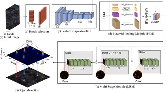
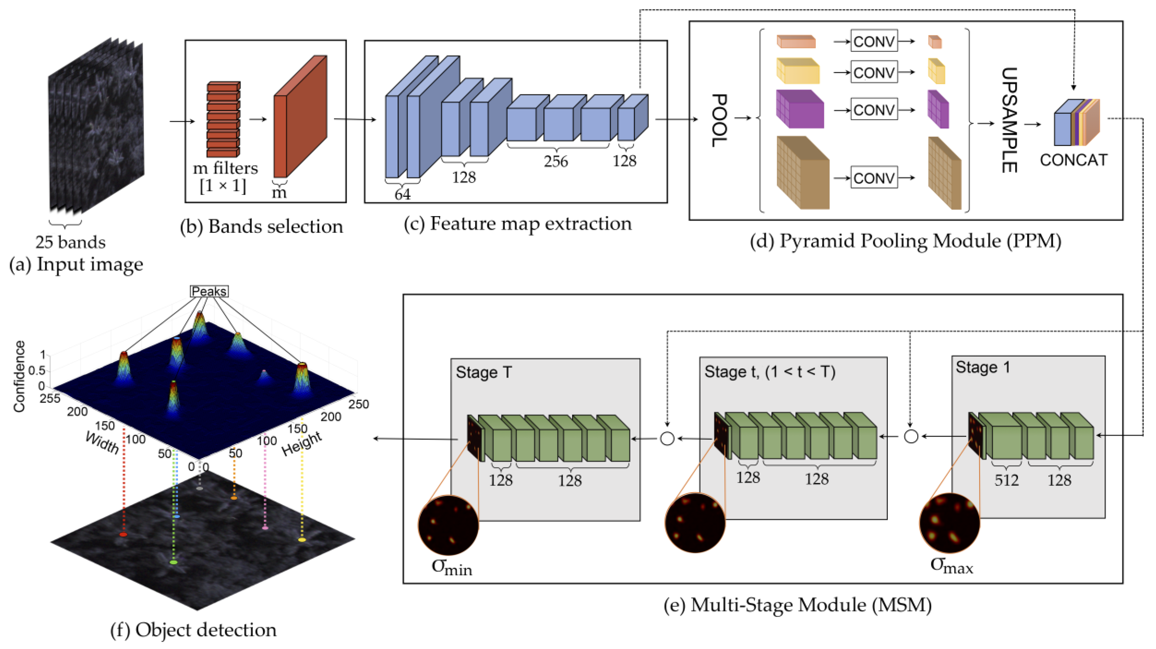
2.3. Proposed Method

The proposed CNN method takes a hyperspectral image as input and computes the individual tree positions. The hyperspectral image has 25 bands with w × h pixels each. The tree identification and location are modeled as a 2D confidence map estimation, following the procedures related in [50,67]. The confidence map is a 2D representation of the likelihood of a tree occurring in each pixel of the image. First, the hyperspectral images go through a band learning process before extracting the feature map. This allows the method to improve its accuracy by learning the best band combination for the trees detection. We included the Pyramid Pooling Module (PPM) [68] that uses global and local information to improve the estimation of the confidence map. Besides, we implemented a multi-stage prediction that refines the confidence map to a more accurate prediction of the center of the trees.
Figure 2 presents our approach for tree detection and geolocation. The method starts with a band-learning module that is responsible for learning m new bands from the hyperspectral image (Figure 2b). Additionally, a feature map (Figure 2c) is extracted using the output volume of the band-learning module. This feature map obtains global and local neighborhood information when passing through the PPM (Figure 2d). The volume is then processed by a Multi-Stage Module (MSM) (Figure 2e) with T stages to refine the tree detection. Finally, we obtain the trees’ positions (Figure 2f) at the end of the method.
The following sections detail the main modules of the proposed method: Section 2.3.1 shows the band learning module; Section 2.3.2 presents the feature map and its enhancement with the PPM module; The refinement of the confidence map by the MSM and the obtaining of the tree positions are presented in Section 2.3.3.

2.3.1. Band Learning Machine Module

To improve the band selection process of our network, we propose an end-to-end band learning module. This module receives a hyperspectral image with w × h pixels and 25 bands and learns m filters with size 1 × 1 × 25 to generate an output image with dimensions w × h × m. Figure 3 illustrates an example of the application of the last filter, represented by the yellow color. Each filter is convolved through the input image (Figure 3a) with a stride of 1 pixel, creating a corresponding output volume (Figure 3c). During training, each filter has its weights adjusted to detect the bands that have more influence on the single-tree detection task. In this way, the layers that have more response in detecting objects will be enhanced, while the others will be discarded in the process.

2.3.2. Feature Map Extraction

The feature map is extracted using a CNN (Figure 2c), based on the VGG19 method [34], from the hyperspectral image learned in the previous step (Section 2.3.1). Our CNN has eight convolutional layers composed of 64, 128 and 256 convolutional filters with size 3 × 3 to consider spatial information. After the second and fourth convolutional layers, we reduce the spatial volume size in half using the max-pooling layer with a 2 × 2 window. In each convolutional layer, we applied a Rectified Linear Units (ReLU) function.
To characterize global and local information from the image, we adopt the PPM [68]. This module aims to make our method invariant to scale, which is important for detecting trees at different scales and even growth stages. The PPM module (Figure 2d) receives the feature map and applies four branches with max-pooling layers, resulting in four volumes with resolutions of 1 × 1, 2 × 2, 3 × 3, and 6 × 6. The general level, shown in orange shown in Figure 2d, creates a feature map that describes the global context of the image while the other branch divides the feature map into subregions to better characterize the local information. The features of each branch are upsampled to the same size as the input feature map and are concatenated with the input feature map to form an improved description of the image.

2.3.3. Tree Localization

The tree’s positions are located using a refined confidence map obtained by the MSM (Figure 2e). The MSM estimates a confidence map from the feature map obtained in the last module (see Section 2.3.2) and is composed of T refinement stages. The first stage contains three layers with 128 convolutional filters of 3 × 3 size, one layer with 512 convolutional filters of 1 × 1 size, and the last layer with a single convolutional filter that corresponds to the confidence map C 1 of the first stage.
The T–1 final stage refines the positions predicted in the first stage, forming hierarchical learning of the trees’ positions. In a stage t ∈ [2, 3, ..., T], the prediction returned by the previous stage C t 1 and the feature map from the PPM module is concatenated and used to produce a refined confidence map C 1 . These stages have, in total, seven convolutional layers: five layers with 128 filters of 7 × 7 size; and one layer with 128 filters of 1 × 1 size. The last layer has a sigmoid activation function so that each pixel represents the probability of the occurrence of a tree (with values between [0, 1]). The remaining layers have a ReLU activation function. Additionally, the use of the improved feature map at the entrance of each stage allows multi-scale features, obtained from global and local context information, to be incorporated into the refinement process.
Later, to avoid the vanishing gradient problem during the training phase, we adopted a loss function at the end of each stage as shown in the following Equation (1).
f t = p C ^ t ( p ) C t ( p ) 2 2 ,
where C ^ t and C t are, respectively, the ground truth and the refined confidence maps of the location p at stage t. The general loss functions are given by:
f = t = 1 T f t ,
To train our approach, a confidence map C ^ t is generated as the ground truth for each stage t using the annotations of the trees. The ground-truth confidence map is generated by placing a 2D Gaussian kernel at the labeled tree centers. The Gaussian kernel has a standard deviation σ t that controls the spread of the peak. Our approach uses different values of σ t for each stage t to refine the tree prediction during each stage. The σ 1 of the first stage is set to a maximum value σ m a x while the σ T of the last stage is set to a minimum value σ m i n . The σ t for each intermediate stage is equally spaced between [ σ m a x , σ m i n ]. During the early phase of our experiment, the usage of different σ helped to refine the confidence map, improving its robustness.
The tree’s locations are then obtained from the last stage C T of the MSM module. For the tree location we estimate the peaks (local maximum) of the confidence map by analyzing the 4-pixel neighborhood of each given location of p . Thus, p = ( x p ,   y p ) is a local maximum if C T ( p ) > C T ( v ) for all the neighbors v , where v is given by ( x p ± 1 ,   y p ) or ( x p ,   y p   ± 1 ) . An example of the tree location from the confidence map peaks is shown in Figure 4.
To avoid noise or low probability of occurrence of the positions p, a peak in the confidence map is considered as an object only if C T ( p ) > τ . For this, we set a minimum distance δ to prevent the detection of objects very close to each other. After a preliminary experiment, we used δ = 1 pixel and τ = 0.35.

2.4. Experimental Setup

The images were split into patches with 256 × 256 pixels without overlapping. The patches were randomly divided into training, validation and testing sets, in a proportion of 50%, 25%, and 25%, respectively. Figure 5 shows the images used to extract the training, validation and test sets in each year (2016, 2017, and 2018) and Table 2 shows the number of samples. It is noted the different number of samples for each year because of slight differences in the images acquisition. For training, we initialized the first part weights of our network with pre-trained weights on ImageNet and applied a stochastic gradient descent optimizer with a moment of 0.9. The validation set was used to adjust the learning rate and the number of epochs, reducing the risk of overfitting in our method. After the adjustments, the learning rate was set to 0.001 and the number of epochs was set to 100. The proposed approach was implemented in Python on Ubuntu 18.04 operating system and used the Keras-Tensorflow API. The workstation used for both training and testing has an Intel (R) Xeon (E) E3-1270\@3.80 GHz CPU, 64 GB memory and an NVIDIA Titan V graphics card, that includes a 5120 CUDA (Compute United Device Architecture) cores and 12 GB of graphics memory. Lastly, to evaluate the performance of the approaches, we adopted three metrics: precision, recall, and f-measure [69]. They were calculated for the 311 tree samples (Table 2) which were not used in the previous steps.

3. Results

3.1. Validation of the Parameters
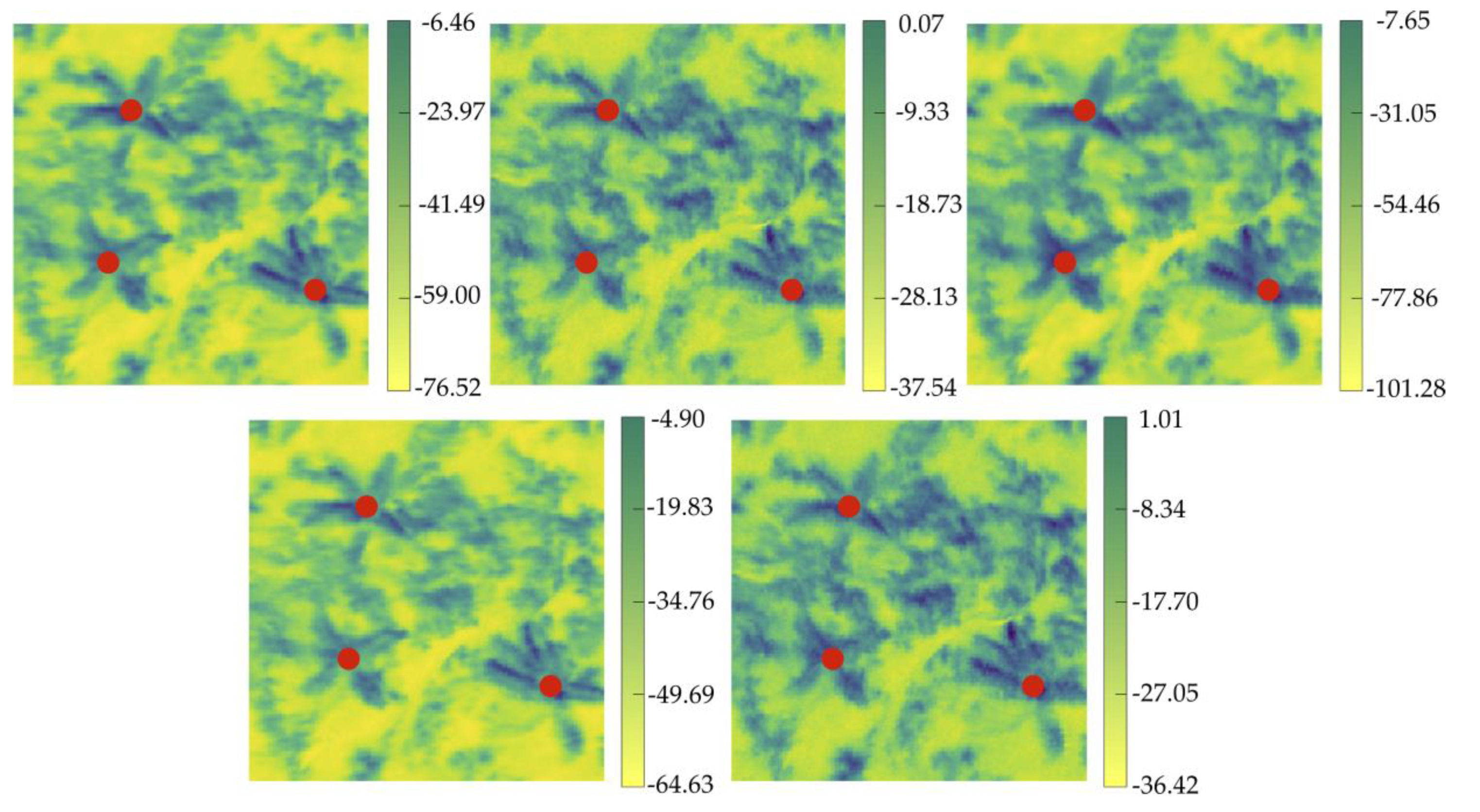
We first evaluate the influence of the proposed method parameters using only the validation images and reported the average f-measure of the three years. Parameters σ m i n , σ m a x and the number of stages, responsible for the refinement task in the density map prediction, were evaluated in the data displayed in Figure 6. From the f-measured shown in Figure 6a, σ m i n = 1 obtained the best result. Smaller values in this graphic represent a small spread of the density maps’ peak around the center of the trees, thus impairing their detection. On the other hand, higher values of σ m i n in the last stage of our method returns a large spread that can cover more than one tree per area. In this sense, only one tree would be detected instead of two, as an example. As shown in Figure 4, σ m a x may be larger since it determines the density map of the first stage that is refined in the subsequent stages. This parameter can be situated between 2.8 and 3.2, although the best value in the experiment was 3 (Figure 6b). The number of stages n ranged from 2 to 8 as shown in Figure 6c. We found that n = 6 achieved the highest overall f-measure. In this manner, the refinement step of our network used the following parameters: σ m i n = 1 , σ m a x = 3 , and n = 6 .
The input images in the experiment have a total of 25 spectral bands. Our method can detect how many of them contributed effectively to the tree detection task. We then evaluated the proposed convolutional layer for learning m linear band combinations in Figure 7. The experiment showed that the number of band combinations m = 5 reached the best f-measure of 0.939 against 0.892 when considering all the 25 spectral bands. The data shows that adding more linear combinations does not improve the results. These results confirm that the proposed layer appropriately combines which bands should be considered while avoiding the correlation and the scarcity that hinder most deep learning methods.
Figure 8 shows an example of the m = 5 linear band combinations. As displayed, these 5 new bands highlighted in blue the target of interest. The point in red represents the labeled ground-truth. The values range from 0 (yellow) to 1 (blue), and our object of interest presents the highest values.

3.2. Band Analysis

To determine the robustness of the band selection module as an initial step of our network, we performed a comparison with our network baseline (i.e., every step beyond the feature map extraction, Figure 2) and different inputs. One input consisted of all the 25 spectral bands, whereas the other input was composed of spectral bands obtained through a PCA approach. It is also important to emphasize that the results of this section were obtained from the test images, whereas the parameters of the methods were estimated from the validation set. Additionally, the PCA contained 99. 27% of the total information.
Table 3 displays the overall precision, recall, and f-measure for the test images in the different scenarios described in the previous paragraph. By analyzing the precision values, it is evident that the baseline of our method in conjunction with the PCA spectral bands returned higher values when in comparison with the baseline plus all 25 bands. These precision values indicate that they do not have many false positives (i.e., do not detect trees incorrectly). When the recall values are analyzed, the proposed method with the band selection module is better than both approaches. This indicates that the proposed method detects most trees while others fail to detect them in the same manner.
When considering the f-measure, viewed as the harmonic mean of precision and recall, it is observed that the use of all 25 bands was exceeded by the PCA (from 0.889 to 0.921). Compared to the baseline with the 25 spectral bands, the proposed method using five linear band combinations significantly improved the f-measure; from 0.889 to 0.956. Besides, the supervised reduction of bands proposed here proved to be superior to the PCA method, with an increase of 3.8% in f-measure (from 0.921 to 0.959) and 7.4% in recall (from 0.871 to 0.945).
Figure 9 shows a qualitative view of the results of tree detection for the test images obtained in the 2016 and 2018 years. In Figure 9, detected trees have a yellow circle (meaning true-positive) while undetected trees have a red circle (false-negative). The yellow dots indicate incorrect detection by both methods (false-positive). By implementing all bands, the network returned the worst results due to the redundancy of spectral information; corroborating with the Hughes phenomenon. The PCA improved the detection of trees (Figure 9b) although it failed to detect a portion of them, which explains the low recall values when compared to the proposed method. As showcased here, the proposed method was able to detect the majority of trees correctly (Figure 9c).

4. Discussion

The methodological contribution of our CNN based method is evident when comparisons, both quantitatively and qualitatively, are made (Figure 9 and Table 3). The implementation of a band selection module within our network’s architecture not only reduces the amount of noise provoked by the dimensionality of hyperspectral data but also achieved better performance in the proposed task. A comparison with the PCA method, which is a common practice to reduce the number of bands needed, demonstrates the importance of adopting a method that considers the spectral information of the labeled object to select the right number of bands. This feature is not a common procedure for deep neural networks to consider within their architectures, and future methods could benefit from the module proposed here.
Concerning the high-density scene, the remaining process of our network already proved to be effective against other conditions [50]. Nonetheless, this was the first time that we have used a heavily-dense forested environment and hyperspectral data. The PPM module and the MSM stage refinement are important phases since they produce a high-quality density map containing the object’s location. This returns high predictions even when trees are located near each other. In this sense, these modules are important as they enable our method to predict both overlapping and isolated trees (Figure 9c).
Bearing the results of the proposed network baseline in the detecting Syagrus romanzoffiana, it is highlighted the high f-measure value achieved (0.959 as shown in Table 3). This palm tree is essential to forest regeneration [58] and its accurate identification can improve the monitoring of forest successional stages. Additionally, Syagrus romanzoffiana identification can be applied to fauna studies, such as the one related to tapirs monitoring since this mammal is one of the main consumers of this palm tree fruits and spread its seeds by the feces, contributing to the tree species dissemination [55,61].
Moreover, besides the developed method, the Syagrus romanzoffiana characteristics may assist this tree species identification. Results from Miyoshi et al. [17] showed the higher reflectance factor of this tree species when compared with the other seven tree species belonging to the transect area, especially in the near-infrared region of the electromagnetic spectrum. In this region, the vegetation response is mainly affected by the leaf’s cell structure [70] and is an important region to tree species identification [71,72]. Beyond that, there is the unique crown spatial distribution of Syagrus romanzoffiana. Its crown shape is like a star, while the other tree species has umbrella, oval, broad, or irregular shapes among others, not counting the difference in the existence of different layers in these crowns [17].
Lastly, when comparing the results with different researches that applied deep learning, it is noticed that they are consistent with ours. Sothe et al. [23] showed a better performance of CNN than SVM and RF when identifying tree species from the ombrophilous dense forest. Safonova et al. [24] found values of f-measures up to almost 93% when applying data augmentation and CNN in RGB images. Furthermore, Nezami et al. [22] also achieved high precision and recall values (i.e., higher than 0.9) when identifying three tree species using a 3D-CNN. Using the Residual Neural Network (ResNet) and RGB images acquired with UAV over three years, Natesan et al. [73] achieved an average f-measure value of 80% to identify three types of pine trees. The use of deep learning in RGB images is also shown by Santos et al. [32] achieving an average precision of 92% in Dipteryx alata tree species identification. These accuracies demonstrate that our method, with an f-measure equal to 0.959 (Table 3), was also able to return state-of-the-art performance for the detection of tree species in a forest environment.

5. Conclusions

In this paper we presented a novel deep learning method, based upon a CNN architecture, to deal with high dimensionality data of hyperspectral UAV-based images to detect single-tree species. Our approach was constructed with a band selection feature in its initial step. This implementation within the network proved to be appropriate to deal with high dimensionality and was superior when compared with the baseline method considering all the 25 spectral bands and the PCA approach. Our CNN architecture is also followed by a feature map extraction and a multi-stage model refinement of the confidence map. The constructed architecture considers the possibility of every pixel in the image to be correspondent with an actual tree-species. This was important to produce accurate results in a highly-dense scene. The proposed method returned a state-of-the-art performance for detecting and geolocating trees in UAV-based hyperspectral images, with an f-measure, precision and recall values equal to 0.959, 0.973, and 0.945 respectively. Differently from other current deep neural networks, our method estimates a combination of hyperspectral bands that most contribute to the mentioned task within the network’s architecture. The approach demonstrated here is important to deal with forest environment monitoring while providing accurate identification of single-trees.

Author Contributions

Conceptualization, G.T.M., M.d.S.A., L.P.O., J.M.J., D.N.G., N.N.I., A.M.G.T., E.H., and W.N.G.; methodology, M.d.S.A., J.M.J., D.N.G. and W.N.G.; writing—original draft preparation, G.T.M., M.d.S.A., L.P.O., J.M.J., D.N.G., E.H. and W.N.G.; writing—review and editing, G.T.M., M.d.S.A., L.P.O., J.M.J., D.N.G., N.N.I., A.M.G.T., E.H. and W.N.G.; funding acquisition, J.M.J., M.d.S.A., N.N.I., A.M.G.T., E.H. and W.N.G. All authors have read and agreed to the published version of the manuscript.

Funding

This study was financed in part by the Coordenação de Aperfeiçoamento de Pessoal de Nível Superior-Brasil (CAPES)-Finance Code 001, CAPES/PrInt, and CAPES/PDSE, grant number 88881.187406/2018-01; in part by the National Council for Scientific and Technological Development (CNPq), grant number 303559/2019-5, 433783/2018-4, and 153854/2016-2; in part by the São Paulo Research Foundation (FAPESP), grant number 2013/50426-4; and in part by the Academy of Finland, grant number 327861.

Conflicts of Interest

The authors declare no conflict of interest.

References

  1. Aasen, H.; Honkavaara, E.; Lucieer, A.; Zarco-Tejada, P.J. Quantitative Remote Sensing at Ultra-High Resolution with UAV Spectroscopy: A Review of Sensor Technology, Measurement Procedures, and Data Correction Workflows. Remote. Sens. 2018, 10, 1091. [Google Scholar] [CrossRef] [Green Version]
  2. Guimarães, N.; Pádua, L.; Marques, P.; Silva, N.; Peres, E.; Sousa, J.J. Forestry Remote Sensing from Unmanned Aerial Vehicles: A Review Focusing on the Data, Processing and Potentialities. Remote. Sens. 2020, 12, 1046. [Google Scholar] [CrossRef] [Green Version]
  3. Näsi, R.; Honkavaara, E.; Lyytikäinen-Saarenmaa, P.; Blomqvist, M.; Litkey, P.; Hakala, T.; Viljanen, N.; Kantola, T.; Tanhuanpää, T.; Holopainen, M. Using UAV-Based Photogrammetry and Hyperspectral Imaging for Mapping Bark Beetle Damage at Tree-Level. Remote. Sens. 2015, 7, 15467–15493. [Google Scholar] [CrossRef] [Green Version]
  4. Saarinen, N.; Vastaranta, M.; Näsi, R.; Rosnell, T.; Hakala, T.; Honkavaara, E.; Wulder, M.A.; Luoma, V.; Tommaselli, A.M.G.; Imai, N.N.; et al. Assessing Biodiversity in Boreal Forests with UAV-Based Photogrammetric Point Clouds and Hyperspectral Imaging. Remote. Sens. 2018, 10, 338. [Google Scholar] [CrossRef] [Green Version]
  5. Reis, B.P.; Martins, S.V.; Filho, E.I.F.; Sarcinelli, T.S.; Gleriani, J.M.; Marcatti, G.E.; Leite, H.G.; Halassy, M. Management Recommendation Generation for Areas Under Forest Restoration Process through Images Obtained by UAV and LiDAR. Remote. Sens. 2019, 11, 1508. [Google Scholar] [CrossRef] [Green Version]
  6. Navarro, A.; Young, M.; Allan, B.; Carnell, P.; Macreadie, P.; Ierodiaconou, D. The application of Unmanned Aerial Vehicles (UAVs) to estimate above-ground biomass of mangrove ecosystems. Remote. Sens. Environ. 2020, 242, 111747. [Google Scholar] [CrossRef]
  7. Casapia, X.T.; Falen, L.; Bartholomeus, H.; Cárdenas, R.; Flores, G.; Herold, M.; Coronado, E.N.H.; Baker, T.R. Identifying and Quantifying the Abundance of Economically Important Palms in Tropical Moist Forest Using UAV Imagery. Remote. Sens. 2019, 12, 9. [Google Scholar] [CrossRef] [Green Version]
  8. Li, L.; Chen, J.; Mu, X.; Li, W.; Yan, G.; Xie, D.; Zhang, W. Quantifying Understory and Overstory Vegetation Cover Using UAV-Based RGB Imagery in Forest Plantation. Remote. Sens. 2020, 12, 298. [Google Scholar] [CrossRef] [Green Version]
  9. Colgan, M.S.; Baldeck, C.A.; Féret, J.-B.; Asner, G.P. Mapping Savanna Tree Species at Ecosystem Scales Using Support Vector Machine Classification and BRDF Correction on Airborne Hyperspectral and LiDAR Data. Remote Sens. 2012, 4, 3462–3480. [Google Scholar] [CrossRef] [Green Version]
  10. Nevalainen, O.; Honkavaara, E.; Tuominen, S.; Viljanen, N.; Hakala, T.; Yu, X.; Hyyppä, J.; Saari, H.; Pölönen, I.; Imai, N.N.; et al. Individual Tree Detection and Classification with UAV-Based Photogrammetric Point Clouds and Hyperspectral Imaging. Remote. Sens. 2017, 9, 185. [Google Scholar] [CrossRef] [Green Version]
  11. Tuominen, S.; Näsi, R.; Honkavaara, E.; Balazs, A.; Hakala, T.; Viljanen, N.; Pölönen, I.; Saari, H.; Ojanen, H. Assessment of Classifiers and Remote Sensing Features of Hyperspectral Imagery and Stereo-Photogrammetric Point Clouds for Recognition of Tree Species in a Forest Area of High Species Diversity. Remote. Sens. 2018, 10, 714. [Google Scholar] [CrossRef] [Green Version]
  12. Raczko, E.; Zagajewski, B. Comparison of support vector machine, random forest and neural network classifiers for tree species classification on airborne hyperspectral APEX images. Eur. J. Remote. Sens. 2017, 50, 144–154. [Google Scholar] [CrossRef] [Green Version]
  13. Xie, Z.; Chen, Y.; Lu, D.; Li, G.; Chen, E. Classification of Land Cover, Forest, and Tree Species Classes with ZiYuan-3 Multispectral and Stereo Data. Remote. Sens. 2019, 11, 164. [Google Scholar] [CrossRef] [Green Version]
  14. Maxwell, A.E.; Warner, T.A.; Fang, F. Implementation of machine-learning classification in remote sensing: An applied review. Int. J. Remote Sens. 2018, 39, 2784–2817. [Google Scholar] [CrossRef] [Green Version]
  15. Osco, L.P.; Ramos, A.P.M.; Pereira, D.R.; Moriya, É.; Imai, N.N.; Matsubara, E.; Estrabis, N.; De Souza, M.; Marcato, J.; Goncalves, W.N.; et al. Predicting Canopy Nitrogen Content in Citrus-Trees Using Random Forest Algorithm Associated to Spectral Vegetation Indices from UAV-Imagery. Remote. Sens. 2019, 11, 2925. [Google Scholar] [CrossRef] [Green Version]
  16. Pham, T.D.; Yokoya, N.; Bui, D.T.; Yoshino, K.; Friess, D.A. Remote Sensing Approaches for Monitoring Mangrove Species, Structure, and Biomass: Opportunities and Challenges. Remote. Sens. 2019, 11, 230. [Google Scholar] [CrossRef] [Green Version]
  17. Miyoshi, G.T.; Imai, N.N.; Tommaselli, A.M.G.; De Moraes, M.V.A.; Honkavaara, E. Evaluation of Hyperspectral Multitemporal Information to Improve Tree Species Identification in the Highly Diverse Atlantic Forest. Remote. Sens. 2020, 12, 244. [Google Scholar] [CrossRef] [Green Version]
  18. Marrs, J.; Ni-Meister, W. Machine Learning Techniques for Tree Species Classification Using Co-Registered LiDAR and Hyperspectral Data. Remote. Sens. 2019, 11, 819. [Google Scholar] [CrossRef] [Green Version]
  19. Imangholiloo, M.; Saarinen, N.; Markelin, L.; Rosnell, T.; Näsi, R.; Hakala, T.; Honkavaara, E.; Holopainen, M.; Hyyppä, J.; Vastaranta, M. Characterizing Seedling Stands Using Leaf-Off and Leaf-On Photogrammetric Point Clouds and Hyperspectral Imagery Acquired from Unmanned Aerial Vehicle. Forests 2019, 10, 415. [Google Scholar] [CrossRef] [Green Version]
  20. Cao, J.; Leng, W.; Liu, K.; Liu, L.; He, Z.; Zhu, Y. Object-Based Mangrove Species Classification Using Unmanned Aerial Vehicle Hyperspectral Images and Digital Surface Models. Remote. Sens. 2018, 10, 89. [Google Scholar] [CrossRef] [Green Version]
  21. Näsi, R.; Honkavaara, E.; Blomqvist, M.; Lyytikäinen-Saarenmaa, P.; Hakala, T.; Viljanen, N.; Kantola, T.; Holopainen, M. Remote sensing of bark beetle damage in urban forests at individual tree level using a novel hyperspectral camera from UAV and aircraft. Urban For. Urban Green. 2018, 30, 72–83. [Google Scholar] [CrossRef]
  22. Nezami, S.; Khoramshahi, E.; Nevalainen, O.; Pölönen, I.; Honkavaara, E. Tree Species Classification of Drone Hyperspectral and RGB Imagery with Deep Learning Convolutional Neural Networks. Remote. Sens. 2020, 12, 1070. [Google Scholar] [CrossRef] [Green Version]
  23. Sothe, C.; Almeida, C.M.D.; Schimalski, M.B.; Rosa, L.E.C.L.; Castro, J.D.B.; Feitosa, R.Q.; Dalponte, M.; Lima, C.L.; Liesenberg, V.; Miyoshi, G.T.; et al. Comparative performance of convolutional neural network, weighted and conventional support vector machine and random forest for classifying tree species using hyperspectral and photogrammetric data. GIScience Remote. Sens. 2020, 57, 369–394. [Google Scholar] [CrossRef]
  24. Safonova, A.; Tabik, S.; Alcaraz-Segura, D.; Rubtsov, A.; Maglinets, Y.; Herrera, F. Detection of Fir Trees (Abies sibirica) Damaged by the Bark Beetle in Unmanned Aerial Vehicle Images with Deep Learning. Remote. Sens. 2019, 11, 643. [Google Scholar] [CrossRef] [Green Version]
  25. Li, W.; Fu, H.; Yu, L.; Cracknell, A. Deep Learning Based Oil Palm Tree Detection and Counting for High-Resolution Remote Sensing Images. Remote Sens. 2017, 9, 22. [Google Scholar] [CrossRef] [Green Version]
  26. Kamilaris, A.; Prenafeta-Boldú, F.X. Deep learning in agriculture: A survey. Comput. Electron. Agric. 2018, 147, 70–90. [Google Scholar] [CrossRef] [Green Version]
  27. Ma, L.; Liu, Y.; Zhang, X.; Ye, Y.; Yin, G.; Johnson, B.A. Deep learning in remote sensing applications: A meta-analysis and review. ISPRS J. Photogramm. Remote. Sens. 2019, 152, 166–177. [Google Scholar] [CrossRef]
  28. Khamparia, A.; Singh, K. A systematic review on deep learning architectures and applications. Expert Syst. 2019, 36, e12400. [Google Scholar] [CrossRef]
  29. Redmon, J.; Farhadi, A. YOLOv3: An Incremental Improvement. arXiv 2018, arXiv:1804.02767. [Google Scholar]
  30. Lin, T.-Y.; Goyal, P.; Girshick, R.B.; He, K.; Dollár, P. Focal Loss for Dense Object Detection. arXiv 2017, arXiv:1708.02002. [Google Scholar]
  31. Ren, S.; He, K.; Girshick, R.B.; Sun, J. Faster R-CNN: Towards Real-Time Object Detection with Region Proposal Networks. arXiv 2015, arXiv:1506.01497. [Google Scholar]
  32. Dos Santos, A.A.; Marcato Junior, J.; Araújo, M.S.; Di Martini, D.R.; Tetila, E.C.; Siqueira, H.L.; Aoki, C.; Eltner, A.; Matsubara, E.T.; Pistori, H.; et al. Assessment of CNN-Based Methods for Individual Tree Detection on Images Captured by RGB Cameras Attached to UAVs. Sensors 2019, 19, 3595. [Google Scholar] [CrossRef] [Green Version]
  33. Lobo Torres, D.; Feitosa, R.; Nigri Happ, P.; Cue La Rosa, L.; Junior, J.; Martins, J.; Bressan, P.; Gonçalves, W.; Liesenberg, V. Applying Fully Convolutional Architectures for Semantic Segmentation of a Single Tree Species in Urban Environment on High Resolution UAV Optical Imagery. Sensors 2020, 20, 563. [Google Scholar] [CrossRef] [Green Version]
  34. Simonyan, K.; Zisserman, A. Very Deep Convolutional Networks for Large-Scale Image Recognition. arXiv 2015, arXiv:1409.1556. [Google Scholar]
  35. Sylvain, J.-D.; Drolet, G.; Brown, N. Mapping dead forest cover using a deep convolutional neural network and digital aerial photography. ISPRS J. Photogramm. Remote. Sens. 2019, 156, 14–26. [Google Scholar] [CrossRef]
  36. Weinstein, B.G.; Marconi, S.; Bohlman, S.; Zare, A.; White, E. Individual tree-crown detection in RGB imagery using self-supervised deep learning neural networks. bioRxiv 2019. [Google Scholar] [CrossRef] [Green Version]
  37. Hartling, S.; Sagan, V.; Sidike, P.; Maimaitijiang, M.; Carron, J. Urban Tree Species Classification Using a WorldView-2/3 and LiDAR Data Fusion Approach and Deep Learning. Sensors 2019, 19, 1284. [Google Scholar] [CrossRef] [PubMed] [Green Version]
  38. Belgiu, M.; Drăguţ, L. Random forest in remote sensing: A review of applications and future directions. ISPRS J. Photogramm. Remote. Sens. 2016, 114, 24–31. [Google Scholar] [CrossRef]
  39. Hennessy, A.; Clarke, K.; Lewis, M. Hyperspectral Classification of Plants: A Review of Waveband Selection Generalisability. Remote. Sens. 2020, 12, 113. [Google Scholar] [CrossRef] [Green Version]
  40. Alshehhi, R.; Marpu, P.R.; Woon, W.L.; Mura, M.D. Simultaneous extraction of roads and buildings in remote sensing imagery with convolutional neural networks. ISPRS J. Photogramm. Remote. Sens. 2017, 130, 139–149. [Google Scholar] [CrossRef]
  41. Audebert, N.; Saux, B.L.; Lefevre, S. Deep Learning for Classification of Hyperspectral Data: A Comparative Review. IEEE Geosci. Remote Sens. Mag. 2019, 7, 159–173. [Google Scholar] [CrossRef] [Green Version]
  42. Bioucas-Dias, J.; Plaza, A.; Camps-Valls, G.; Scheunders, P.; Nasrabadi, N.M.; Chanussot, J. Hyperspectral Remote Sensing Data Analysis and Future Challenges. IEEE Geosci. Remote Sens. Mag. 2013, 1, 6–36. [Google Scholar] [CrossRef] [Green Version]
  43. Richards, J.A.; Jia, X. Remote Sensing Digital Image Analysis: An Introduction, 4th ed.; Springer: Berlin/Heidelberg, Germany, 2005; ISBN 3-540-25128-6. [Google Scholar]
  44. Maschler, J.; Atzberger, C.; Immitzer, M. Individual Tree Crown Segmentation and Classification of 13 Tree Species Using Airborne Hyperspectral Data. Remote. Sens. 2018, 10, 1218. [Google Scholar] [CrossRef] [Green Version]
  45. Liu, L.; Song, B.; Zhang, S.; Liu, X. A Novel Principal Component Analysis Method for the Reconstruction of Leaf Reflectance Spectra and Retrieval of Leaf Biochemical Contents. Remote. Sens. 2017, 9, 1113. [Google Scholar] [CrossRef] [Green Version]
  46. Johnson, R.A.; Wichern, D.W. Applied Multivariate Statistical Analysis; Pearson Prentice Hall: Upper Saddle River, NJ, USA, 2007; ISBN 978-0-13-187715-3. [Google Scholar]
  47. Özcan, A.H.; Hisar, D.; Sayar, Y.; Ünsalan, C. Tree crown detection and delineation in satellite images using probabilistic voting. Remote Sens. Lett. 2017, 8, 761–770. [Google Scholar] [CrossRef]
  48. Csillik, O.; Cherbini, J.; Johnson, R.; Lyons, A.; Kelly, M. Identification of Citrus Trees from Unmanned Aerial Vehicle Imagery Using Convolutional Neural Networks. Drones 2018, 2, 39. [Google Scholar] [CrossRef] [Green Version]
  49. Ampatzidis, Y.; Partel, V. UAV-Based High Throughput Phenotyping in Citrus Utilizing Multispectral Imaging and Artificial Intelligence. Remote. Sens. 2019, 11, 410. [Google Scholar] [CrossRef] [Green Version]
  50. Osco, L.P.; Arruda, M.D.S.D.; Junior, J.M.; Da Silva, N.B.; Ramos, A.P.M.; Moryia, É.A.S.; Imai, N.N.; Pereira, D.R.; Creste, J.E.; Matsubara, E.T.; et al. A convolutional neural network approach for counting and geolocating citrus-trees in UAV multispectral imagery. ISPRS J. Photogramm. Remote. Sens. 2020, 160, 97–106. [Google Scholar] [CrossRef]
  51. Brasil Descreto s/n de 16 de julho de 2002. 2002. Available online: http://www.planalto.gov.br/ccivil_03/dnn/2002/Dnn9609.htm (accessed on 15 October 2016).
  52. Brasil Descreto s/n de 14 de maio de 2004. 2004. Available online: http://www.planalto.gov.br/CCIVIL_03/_Ato2004-2006/2004/Decreto/_quadro.htm (accessed on 15 October 2016).
  53. Berveglieri, A.; Tommaselli, A.M.G.; Imai, N.N.; Ribeiro, E.A.W.; Guimarães, R.B.; Honkavaara, E. Identification of Successional Stages and Cover Changes of Tropical Forest Based on Digital Surface Model Analysis. IEEE J. Sel. Top. Appl. Earth Obs. Remote. Sens. 2016, 9, 5385–5397. [Google Scholar] [CrossRef]
  54. Berveglieri, A.; Imai, N.N.; Tommaselli, A.M.G.; Casagrande, B.; Honkavaara, E. Successional stages and their evolution in tropical forests using multi-temporal photogrammetric surface models and superpixels. ISPRS J. Photogramm. Remote. Sens. 2018, 146, 548–558. [Google Scholar] [CrossRef]
  55. Giombini, M.I.; Bravo, S.P.; Sica, Y.V.; Tosto, D.S. Early genetic consequences of defaunation in a large-seeded vertebrate-dispersed palm (Syagrus romanzoffiana). Heredity 2017, 118, 568–577. [Google Scholar] [CrossRef]
  56. Elias, G.; Colares, R.; Rocha Antunes, A.; Padilha, P.; Tucker Lima, J.; Santos, R. Palm (Arecaceae) Communities in the Brazilian Atlantic Forest: A Phytosociological Study. Floresta e Ambiente 2019, 26. [Google Scholar] [CrossRef]
  57. Da Silva, F.R.; Begnini, R.M.; Lopes, B.C.; Castellani, T.T. Seed dispersal and predation in the palm Syagrus romanzoffiana on two islands with different faunal richness, southern Brazil. Stud. Neotrop. Fauna Environ. 2011, 46, 163–171. [Google Scholar] [CrossRef]
  58. Brasil, D.F. Espécies Nativas da Flora Brasileira de Valor Econômico Atual ou Potencial: Plantas para o Futuro-Região Centro-Oeste. 2011. Available online: https://www.alice.cnptia.embrapa.br/handle/doc/1073295 (accessed on 3 March 2020).
  59. Lorenzi, H. Árvores Brasileiras, 1st ed.; Instituto Plantarum de Estudos da Flora: Nova Odessa, Brazil, 1992; Volume 1, ISBN 85-86714-14-3. [Google Scholar]
  60. Mendes, C.; Ribeiro, M.; Galetti, M. Patch size, shape and edge distance influence seed predation on a palm species in the Atlantic forest. Ecography 2015, 39. [Google Scholar] [CrossRef]
  61. Sica, Y.; Bravo, S.P.; Giombini, M. Spatial Pattern of Pindó Palm (Syagrus romanzoffiana) Recruitment in Argentinian Atlantic Forest: The Importance of Tapir and Effects of Defaunation. Biotropica 2014, 46. [Google Scholar] [CrossRef]
  62. Honkavaara, E.; Saari, H.; Kaivosoja, J.; Pölönen, I.; Hakala, T.; Litkey, P.; Mäkynen, J.; Pesonen, L. Processing and Assessment of Spectrometric, Stereoscopic Imagery Collected Using a Lightweight UAV Spectral Camera for Precision Agriculture. Remote Sens. 2013, 5, 5006–5039. [Google Scholar] [CrossRef] [Green Version]
  63. Honkavaara, E.; Rosnell, T.; Oliveira, R.; Tommaselli, A. Band registration of tuneable frame format hyperspectral UAV imagers in complex scenes. ISPRS J. Photogramm. Remote. Sens. 2017, 134, 96–109. [Google Scholar] [CrossRef]
  64. Honkavaara, E.; Khoramshahi, E. Radiometric Correction of Close-Range Spectral Image Blocks Captured Using an Unmanned Aerial Vehicle with a Radiometric Block Adjustment. Remote. Sens. 2018, 10, 256. [Google Scholar] [CrossRef] [Green Version]
  65. Smith, G.M.; Milton, E.J. The use of the empirical line method to calibrate remotely sensed data to reflectance. Int. J. Remote Sens. 1999, 20, 2653–2662. [Google Scholar] [CrossRef]
  66. Miyoshi, G.T.; Imai, N.N.; Tommaselli, A.M.G.; Honkavaara, E.; Näsi, R.; Moriya, É.A.S. Radiometric block adjustment of hyperspectral image blocks in the Brazilian environment. Int. J. Remote Sens. 2018, 39, 4910–4930. [Google Scholar] [CrossRef] [Green Version]
  67. Aich, S.; Stavness, I. Improving Object Counting with Heatmap Regulation. arXiv 2018, arXiv:1803.05494. [Google Scholar]
  68. Zhao, H.; Shi, J.; Qi, X.; Wang, X.; Jia, J. Pyramid Scene Parsing Network. In Proceedings of the 2017 IEEE Conference on Computer Vision and Pattern Recognition (CVPR), Honolulu, HI, USA, 21–26 July 2017; pp. 6230–6239. [Google Scholar]
  69. Story, M.; Congalton, R.G. Accuracy assessment: A user’s perspective. Photogramm. Eng. Remote Sens. 1986, 52, 397–399. [Google Scholar]
  70. Jensen, J.R. Remote Sensing of the Environment: An Earth Resource Perspective; Prentice Hall Series in Geographic Information Science; Pearson Prentice Hall: Upper Saddle River, NJ, USA, 2007; ISBN 978-0-13-188950-7. [Google Scholar]
  71. Clark, M.L.; Roberts, D.A. Species-Level Differences in Hyperspectral Metrics among Tropical Rainforest Trees as Determined by a Tree-Based Classifier. Remote Sens. 2012, 4, 1820–1855. [Google Scholar] [CrossRef] [Green Version]
  72. Dalponte, M.; Bruzzone, L.; Gianelle, D. Tree species classification in the Southern Alps based on the fusion of very high geometrical resolution multispectral/hyperspectral images and LiDAR data. Remote. Sens. Environ. 2012, 123, 258–270. [Google Scholar] [CrossRef]
  73. Natesan, S.; Armenakis, C.; Vepakomma, U. RESNET-Based tree species classification using UAV images. Int. Arch. Photogramm. Remote Sens. Spat. Inf. Sci. 2019. [Google Scholar] [CrossRef] [Green Version]
Figure 1. Study area in (a) Brazil, (b) São Paulo, (c) the western region of the São Paulo state, and (d) Ponte Branca forest fragment.
Remotesensing 12 01294 g001
Figure 2. Proposed method for tree detection. The first module (b) is responsible for learning m bands from the input image (a). The initial part (c) obtains a feature map from the input image and it is enhanced by the PPM (d). The resulting volume is used as input to the MSM (e). The T stages refine prediction positions until trees (f) are detected.
Remotesensing 12 01294 g002
Figure 3. Band learning module structure. The multispectral image (a) is convolved with m filters with size 1 × 1 × 25 (b) that generate an output volume (c) with m bands.
Remotesensing 12 01294 g003
Figure 4. Example of the tree localization from a refined confidence map.
Remotesensing 12 01294 g004
Figure 5. Image parts used for (a) training, (b) validation and (c) test.
Remotesensing 12 01294 g005
Figure 6. Evaluation of (a) σ m i n = 1 , (b) σ m a x = 3 , and (c) number of stages responsible for the refinement of the density map prediction.
Remotesensing 12 01294 g006
Figure 7. Evaluation of the number of linear band combinations m.
Remotesensing 12 01294 g007
Figure 8. Example of the five linear band combinations obtained by the proposed method.
Remotesensing 12 01294 g008
Figure 9. Qualitative results of the tree detection using (a) all 25 bands, (b) PCA, and the (c) proposed method for the 2016 and 2018 images. The yellowish trees were correctly detected, while the redder ones were undetected.
Remotesensing 12 01294 g009
Table 1. Spectral setting of the Rikola camera. λ represents the central wavelength and FWHM is the full width at half maximum. Both values in nanometers (nm).
Bandλ/FWHMBandλ/FWHMBandλ/FWHMBandλ/FWHMBandλ/FWHM
1506.22/12.446580.16/15.9511650.96/14.4416700.28/18.9421750.16/17.97
2519.94/17.387591.90/16.6112659.72/16.8317710.06/19.7022769.89/18.72
3535.09/16.848609.00/15.0813669.75/19.8018720.17/19.3123780.49/17.36
4550.39/16.539620.22/16.2614679.84/20.4519729.57/19.0124790.30/17.39
5565.10/17.2610628.73/15.3015690.28/18.8720740.42/17.9825819.66/17.84
Table 2. Number of training, validation and test samples used in each experiment.
201620172018Total
Training106174175455
Validation81112112305
Test79116116311
Table 3. Comparative results between the proposed method and PCA in the test images.
MethodPrecisionRecallF-Measure
Baseline + 25 bands0.8980.8810.889
Baseline + PCA (5 bands)0.9790.8710.921
Proposed method0.9730.9450.959

