Combining Genetic Analysis and Multivariate Modeling to Evaluate Spectral Reflectance Indices as Indirect Selection Tools in Wheat Breeding under Water Deficit Stress Conditions

Abstract

Progress in high-throughput tools has enabled plant breeders to increase the rate of genetic gain through multidimensional assessment of previously intractable traits in a fast and nondestructive manner. This study investigates the potential use of spectral reflectance indices (SRIs; 15 vegetation-SRIs; 15 water-SRIs) as alternative selection tools for destructively measured traits in wheat breeding programs. The genetic variability, heritability (h²), genetic gain (GG), and expected genetic advances (GA) of these indices were compared with those of destructively measured traits in 43 F_7-8 recombinant inbred lines (RILs) grown under limited water conditions. The performance of SRIs to estimate the destructively measured traits directly was also evaluated using the partial least squares regression (PLSR) and stepwise multiple linear regression (SMLR) models. Most vegetation-SRIs exhibited high genotypic variation, similar to the measured traits, and phenotypic correlations with these traits, compared with the water-SRIs. Most vegetation-SRIs presented comparable values for h² (>60%) and GG (>20%) as intermediate traits, while about half of water-SRIs exhibited a high h² (>60%), but low GG (<20%). Principle component analysis revealed that most vegetation-SRIs and seven of 15 water-SRIs were grouped together in a positive direction, had a moderate to strong relationship with measured traits, and could identify the drought-tolerant parent Sakha 93 and several RILs. The PLSR model based on all SRIs as a single index showed moderate to high R² in calibration (0.53–0.75) and validation (0.46–0.72) datasets, with strong relationships between observed and predicted values of measured traits. The SMLR models identified four and three SRIs from vegetation-SRIs and water-SRIs, respectively, to explain 63–86% of the total variability in measured traits among genotypes. These results demonstrated that vegetation-SRIs can be used individually or combined with water-SRIs as alternative breeding tools to increase genetic gains and selection accuracy in spring wheat breeding.

1. Introduction

The combination of water shortage and global climate change will increase the occurrence of drought events in arid and semiarid regions, which will become a critical issue for the sustainability of field crop production in such regions. Improving agronomic practices and cultivation of drought-tolerant cultivars are the most feasible strategies to maintain the sustainability of crop production under limited water supply conditions. These strategies aim to maximize crop production per unit of water applied rather than per unit of area [1,2].

Breeding strategies to develop drought-tolerant genotypes rely on the evaluation of several segregating genotypes or crossing lines using multidimensional assessment of phenotypic differences in several plant traits. In-depth multidimensional descriptions of different plant traits, especially under environmental stress, are urgently needed to improve the understanding of the mechanisms underlying adaptive behavior for stress conditions and to provide plant breeders with comprehensive information about the reliability of various components of plant traits as screening criteria for drought tolerance and the ability to incorporate these traits into breeding programs [3,4,5,6]. The first step to develop drought tolerance in breeding programs is to monitor several morpho-physiological plant traits related to drought tolerance for a large number of crossing lines. However, integrative assessments of several plant traits in a large number of genotypes based on plant sampling and traditional measurement techniques is destructive and inefficient. This emphasizes the urgent need to apply the practical, efficient, and economic high-throughput phenotyping tools, which help breeders to assess key plant traits relevant to stress tolerance for a sufficient number of genotypes in a rapid and non-destructive manner comprehensively. Hyperspectral spectroradiometers contain sensors that can detect small changes in biophysical and biochemical characteristics of the canopy by monitoring changes in canopy spectral signatures at the visible (VIS), near-infrared (NIR), and shortwave-infrared (SWIR) parts of the spectrum. They represent an important phenotyping tool in breeding programs and are used to accelerate the development of genotypes for different environmental stress conditions by performing fast, in-depth phenotypic assessments of various phenological plant traits in multiple genotypes [7,8,9,10].

The concept behind this phenotyping tool is that the behavior of spectral reflectance from the canopy at certain wavelengths in the VIS-SWIR domains of the spectrum is strongly affected by substantial changes that take place in specific plant characteristics. These include changes in photosynthetic efficiency, aboveground biomass, internal leaf structures, leaf pigment content, green leaf area index (LAI), plant water content, and other characteristics related to the growth and physiological states of the canopy. For example, changes in the LAI and fresh and dry aboveground biomass impact the spectral reflectance at 760–1300 nm in spring and winter wheat crop [11,12,13]. Changes in the internal leaf structures due to decreases in leaf relative water content impact the spectral reflectance in the red edge (680–740 nm) and NIR (740–940 nm) regions and increase spectral reflectance in the VIS-NIR regions (400–1300 nm) in wheat and maize crops [14,15,16]. Cochavi et al. [17] reported that changes in photosynthetic pigments and function significantly changed the reflectance of the 680 and 740 nm wavelengths in sunflower crop. The spectral reflectance at several specific wavelengths in the NIR and SWIR regions (i.e., wavelengths centered at approximately 970, 1100, 1200, 1240, 1400, 1450, 1665, 1730, 1950, 2100, 2250, and 2500 nm) was strongly associated with changes in leaf water status in wheat, cotton, and grass crops [18,19,20,21,22,23]. Consequently, the close association between canopy spectral reflectance signatures at specific wavelengths in the VIS, NIR, and SWIR parts of the spectrum and different plant characteristics indicates that the plant spectral reflectance tool can be exploited for integrative assessment of several plant traits of a large number of genotypes in an inexpensive, fast, and nondestructive manner. However, associations between spectral reflectance characteristics and different morpho-physiological properties of plants are usually determined through different specific spectral reflectance indices (SRIs), which are computed from the reflectance at given wavelengths using simple mathematical equations, such as ratios, differences, and sums.

Several SRIs have proven useful in the assessment of different morpho-physiological and agronomic parameters, such as LAI, green area index (GAI), aboveground biomass, photosynthetic capacities, chlorophyll content, grain yield, and different traits related to canopy water content in stressed and healthy plants [24,25,26,27,28,29,30]. Among these, the most commonly used indices to assess plant traits related to growth and yield status are the normalized difference vegetation index (NDVI = [R_NIR − R_Red]/[R_NIR + R_Red]) and the simple ratio (SR = [R_NIR/R_Red]. The simple water index (SWI) and different normalized water indices (NWIs), which focus on the minor water absorption bands within the NIR spectrum (970 nm), have been used to assess parameters related to plant water status at both the leaf and canopy levels. Because the detection of canopy spectral signatures by a spectroradiometer is limited by different soil background conditions, such as soil color and moisture, and is very sensitive to some vegetation biophysical parameters, such as LAI, some SRIs have been developed and modified to reduce the impact on the accuracy of this phenotypic tool. Examples of such indices are the optimized soil-adjusted vegetation index (OSAVI, [31]), enhanced vegetation index (EVI, [32]), modified transformed vegetation index (MTVI, [33]), and modified chlorophyll absorption ratio index (MCARI, [34]). Thus, these indices are able to estimate several traits related to growth and grain yield for different crops and conditions.

The ability of different SRIs to assess various phenological plant traits indicates that these indices may be used as indirect selection tools, replacing destructive and direct traditional phenological selection criteria in breeding trials related to drought studies. In addition, the close relationship between SRIs and phenological plant traits may also identify a true genetic relationship and may therefore help plant breeders reliably evaluate thousands of genotypes in a fast and nondestructive manner after successful incorporation in breeding programs [5,9,24,35,36].

Although it is unclear how different SRIs can estimate the performance of different genotypes based on destructively measured phenological plant traits, particularly under abiotic stress conditions, the existence of a statistical and genetic relationship between the indices and destructively measured plant traits is a proof of concept for the adequacy of these indices as an indirect selection tool. Using SRIs as an indirect selection tool in breeding programs is acceptable if the genetic correlation between these indices and the destructively measured plant traits is very high, and if the heritability of these indices is generally greater than that of the destructively measured traits, especially grain yield [9,24,35,36]. These two features of genetic and other analyses enable plant breeders to determine the efficiency of SRIs as alternative indirect selection tools for destructively measured traits among breeding trials in the future. The different SRIs will be more efficient as indirect selection tools in breeding programs if the genetic analyses for SRIs are conducted on genetic populations closely representing the area where the improvement is being targeted. A comprehensive study is thus urgently required to determine the usefulness of SRIs as indirect selection tools to increase the chance of recognizing wheat genotypes that are well adapted to water shortage under arid conditions.

SRIs focus on only two–three wavelengths, reducing the accuracy of indirect estimates of destructively measured traits by a single SRI. Therefore, several studies have focused on multivariate analysis techniques, such as partial least squares regression (PLSR), which deal with a large number of SRIs as a single independent index, to provide more flexibility in the direct estimation of destructively measured traits [28,37,38,39]. Importantly, because the PLSR tool can create reliable models when the number of SRIs (independent variables) greatly exceeds the number of measured traits (dependent variables), several studies have applied this tool to estimate different measured traits accurately, such as LAI, aboveground biomass, photosynthetic capacities, pigment contents, grain yield, and water relation traits [5,29,40,41].

Therefore, the main objectives of this study were: to (1) evaluate the potential use of different SRIs as alternative indirect breeding tools for breeding purposes under limited water irrigation conditions based on their genetic variability, heritability, genetic gain, and expected genetic advances in advanced breeding wheat lines; (2) evaluate the performance of different PLSR models based on all SRIs as a single index for the accurate estimation of measured traits; and (3) select the most influential SRIs that explain most variability in each destructively measured trait across genotypes via a stepwise multiple linear regression analysis.

2. Materials and Methods

2.1. Plant Materials and Field Experiment

A set of 43 F_7–8 recombinant inbred lines (RILs), which were derived by single plant descent to F8 from a hybrid of the drought-tolerant genotype Sakha 93 and the drought-sensitive genotype Sakha 61, was evaluated with their two parents under limited water irrigation conditions during 2014/2015 (F7) and 2015/2016 (F8). The experiments were planted at the Dierab Research Station of the College of Food and Agriculture Sciences, King Saud University, Riyadh, Saudi Arabia (24°25′N, 46°34′E) (Supplementary Figure S1). The soil texture of the experimental area was sandy loam with a bulk density of 1.50 g cm⁻³, along with a field water capacity and wilting point of 0.220 and 0.101 m³ m⁻³, respectively. The soil was characterized as being slightly alkaline (pH 7.9) with low organic matter content (7.8 g kg⁻¹). The average monthly temperature during the growing period (December, January, February, March, and April), was 16.4, 14.6, 17.5, 21.5, and 26.9°C, respectively, and the average monthly precipitation was 12.0, 11.9, 10.0, 11.0, and 3.8 mm, respectively.

Each genotype was planted in 10 row plots at a seeding rate of 150 kg ha⁻¹ with a plot size 1.5 m in width and 4 m in length. The seeds of each genotype were planted in the middle of December in each season. The genotypes were distributed randomly in the plots and arranged in a randomized complete block design with a total of 135 plots. The amount of phosphorus, nitrogen, and potassium fertilizers in each plot were calculated based on the rates of 31, 180, and 120 kg ha⁻¹ of P₂O₅, N, and K₂O, respectively. The entire dose of phosphorus with 20% of nitrogen was applied 2 weeks after sowing, while 40% of nitrogen and half the dose of potassium were applied in the middle of tillering. The remaining dose of nitrogen and potassium was applied at the beginning of the booting growth stage.

Limited water irrigation was applied at a rate of 0.60 of the estimated crop evapotranspiration (ETc). The ETc was estimated based on the crop coefficient (Kc) of spring wheat and the daily reference evapotranspiration (ETo). The Kc values for spring wheat as recommended by FAO-56 were used after adjusting with the actual values of relative humidity and wind speed for the study area. The ETo was calculated by applying the daily meteorological data to the FAO-56 Penman–Monteith equation given by Allen et al. [42]. Based on this calculation, the cumulative amount of irrigation was approximately 3600 m³ ha⁻¹, being equivalent to 360 mm ha⁻¹. About 45 and 40 mm ha⁻¹ of water were applied at sowing and 15 days after sowing, respectively, to ensure full germination and complete establishment of seedlings. Limited water irrigation treatment was started 4 weeks after sowing. The amount of water was applied at the Zadoks growth stages (ZS) of ZS 24, ZS 32, ZS 37, ZS 49, ZS 59, ZS 68, ZS 73, and ZS 83, which referred to the tillering, stem elongation, flag leaf emergence, booting, heading, complete emergence of inflorescence, grain milk, and grain dough of the wheat growth stage, respectively [43]. The irrigation water was applied using a low-pressure surface irrigation system, which had one water emitting tube per plot. To control the amount of irrigation water delivered to each plot, the sub-main hose at each plot was equipped with a manual control valve. The amount of water delivered for each plot was monitored by a flow meter, which connected at the location where the main line encountered the main water source (Supplementary Figure S1).

2.2. Measurements of Plant Traits

At the middle anthesis growth stage (ZS 65), thirty plants from the second and ninth row of each plot were randomly selected to determine the green leaf area (GLA), total dry weight (TDW), and leaf area index (LAI). All the green leaves from 30 plants were separated and run through an area meter (LI 3100; LI-COR Inc., Lincoln, NE, USA) to calculate the surface GLA. Thereafter, all parts of the 30 plants (stem, green and complete brown leaves, and spike) were oven-dried at 70 °C for 72 h and then weighed to obtain TDW.

Data of the total GLA (A), the number of plants in 1 m (B), the number of plants sampled (C = 30, in this study), and the row spacing (D = 15 cm, in this study) were applied using the following equation to calculate the LAI [27]:

$$\mathrm{LAI}=\frac{\mathrm{A}\times \mathrm{B}}{\mathrm{C}\times \mathrm{D}},$$

(1)

Stomatal conductance (Gs) and relative water content (RWC) were measured using the flag leaf of 10 randomly selected plants per plot. The Gs trait was measured at 10:00–13:30 AM using an AP4 diffusion porometer (Delta-T Devices, Cambridge, U.K.). An area of approximately 7–10 cm² from the leaves used to measure Gs was excised, and the fresh weight (FW) was immediately recorded. Then, the leaf samples were rehydrated in deionized water at 25 °C until they were fully turgid and rubbed carefully between paper towels to remove external water from the leaf surface before they were weighed to record the turgid weight (TW). Finally, the dry weight (DW) of the leaf samples was recorded after being oven-dried at 70 °C for 72 h. The data of FW, TW, and DW were applied to the following equation to calculate the RWC:

$$\mathrm{RWC}=\frac{\mathrm{FW}-\mathrm{DW}}{\mathrm{TW}-\mathrm{DW}}\times 100,$$

(2)

After the plants reached maturity, fifty spikes from the third row of each plot were randomly selected and air-dried until the water content reached approximately 15–16% to determine the spike weight (SPW). The five internal rows in each plot, each 3 m in length, were harvested and air-dried for 5 days and then weighed to record the total biological yield (BY). Next, all spikes were separated and threshed, and the final grain yield (GY) was determined. BY and GY values were applied to the following equation to calculate the harvest index (HI) after BY and GY were expressed as ton ha⁻¹:

$$\mathrm{HI}=\frac{\mathrm{GY}}{\mathrm{BY}}$$

(3)

2.3. Spectral Reflectance Measurements

The spectral reflectance of the whole canopy was measured at ZS 65, simultaneous to the GLA and TDW measurements using a portable high-spectral-resolution spectroradiometer (Fieldspec4, Analytical Spectral Devices Inc., Boulder, CO, USA). This spectroradiometer is able to collect reflectance from the canopy at 350–2500 nm of the light spectrum with finally 1.0 nm band intervals (Supplementary Figure S1). The reflectance of the canopy was determined under cloudless and windless conditions between 10:00 and 14:00. The optical fiber of the sensor was held approximately 80 cm above the plant in the nadir direction with a 25° field of view to sense a sufficient area of the wheat canopy (~23.4 cm in diameter). Before and as needed during the spectral reflectance measurements, the incoming reflectance from the plant was calibrated using the Spectralon white reference panel (Labsphere, Inc., North Sutton, NH, USA) coated with BaSO₄. Reflectance was measured from the five internal rows in each plot at four random places, each representing an average of 10 scans, while the average of four sequential measurements and 10 scans per plot was used to estimate 30 spectral reflectance indices (SRIs). These SRIs covered 15 vegetation-SRIs related to the status of growth vigor and photosynthetic efficiency and 15 water-SRIs related to canopy water status, internal leaf structure, and leaf biochemical compounds. The full name, abbreviation, formula, and references of these SRIs are presented in

Table 1. Full name and abbreviation of the vegetation- and water-spectral reflectance indices (vegetation-SRIs and water-SRIs) used in this study and their algorithms and references.

Vegetation-SRIs	Algorithm	Ref.
Normalized difference vegetation index (NDVI)	(R750 − R705)/(R750 + R705)	[44]
Green normalized difference vegetation index (GNDVI)	(R780 − R550)/(R780 + R550)	[45]
Red normalized difference vegetation index (RNDVI)	(R780 − R670)/(R780 + R670)	[46]
Photochemical reflectance index (PRI)	(R531 − R570)/(R531 + R570)	[47]
Green chlorophyll index (GCI)	(R800/R550) − 1	[48]
Normalized phaeophytization index (NPQ)	(R415 − R435)/(R415 + R435 )	[49]
Red-edge model index (RM)	(R750/R720) − 1	[48]
Simple ratio pigment index (SRPI)	(R430/R680)	[50]
Modified chlorophyll absorption ratio index (MCARI)	[(R700 − R670) − 0.2 × (R700 − R550)] × (R700/R670)	[51]
Transformed vegetation index (TVI)	0.5 × [120 × (R750 − R550) − 200 × (R670 − R550)]	[52]
Modified transformed vegetation index (MTVI)	1.2 × [(1.2 × (R800 − R550) − 2.5 × (R670 − R550)]	[33]
Optimized soil adjusted vegetation index (OSAVI)	1.16 × (R800 − R670)/(R800 + R670 + 0.16)	[31]
Red edge inflection point (REIP)	700 + 40 × [(R670 + R780)/2 − R700]/(R740 − R700)	[53]
Structure insensitive pigment index (SIPI)	(R800 − R445 )/(R800 + R680)	[50]
Enhanced vegetation index-2 (EVI-2)	2.5 [(R800 − R660)/(1 + R800 + 2.4 × R660)]	[32]
Water-SRIs
Water index (WI)	(R900/R970)	[54]
Ratio of reflectance between 1000 and 1100 nm (R1000/1100) (R1000/R1100)	(R1000/R1100)	[55]
Normalized water index-1 (NWI-1)	(R970 − R900)/(R970+R900)	[56]
Normalized difference moisture index (NDMI-1)	(R2200 − R1100)/(R2200 + R1100)	[57]
Normalized difference moisture index (NDMI-2)	860 − (R1640 − R2130) / 860 + (R1640 − R2130)	[58]
Normalized difference moisture index-D (NDMI-D)	(R1742 − R1660)/(R1742 + R1660)	[59]
Normalized difference water index-1240 (NDWI1240)	(R860 − R1240)/(R860 + R1240)	[60]
Normalized difference water index-D (NDWI-D)	(R860 − R2270)/(R860 + R2270)	[59]
Shortwave infrared water index (SWWI)	(R850 − R1650)/(R850 + R1650)	[61]
Normalized difference spectral index (NRWC)	(R1222 − R2264)/(R1222 + R2264)	[62]
Development water balance index (WBI-D)	(R1640 − R482)/(R1640 + R482)	[59]
Dry matter content index-D (DMCI-D)	(R2305 − R1550)/(R2305 + R1550)	[59]
Cellulose absorption index (CAI)	0.5 × (R2031 − R2211) − R2101	[63]
Normalized difference lignin index (NDLI)	[log (1/R1754) − log (1/R1680)]/[log (1/R1754) + log (1/R1680)]	[64]
Ligno-cellulose absorption index (LCA)	2 R2205 − (R2165 + R2330)	[65]

.

2.4. Data Analysis

Combined analysis of variance for different destructively measured traits and SRIs were performed across seasons based on a randomized complete block design. Combined ANOVA was performed to analyze the genotypic differences across seasons using Bartlett’s test and the Shapiro–Wilk test for homogeneity of variances and the normality distribution of the residuals, respectively. Based on this test, the results indicated homogenous variance across seasons for both destructively measured traits and SRIs, and therefore, the data of two seasons were combined and analyzed using the CoStat system for Windows, Version 6.311 (CoHort software, Berkeley, CA 94701). The PROC MIXED model for an across seasons combined analysis of variance was conducted as follows:

$$y_{ijk}=\mu +s_i+g_j+s{g}_{ij}+r_{k\left(i\right)}+{\epsilon }_{ijk}$$

(4)

where y is the phenotypic observation of the genotype for the trait of interest, μ is the overall mean, s_i is the effect of the ith season, g_j is the effect of the jth genotype, sg_ij is the interaction effect between season i and genotype j, r_k(i) is the effect of the k^th replication nested within season, and ε_ijk is the residual error and was assumed to be normally and independently distributed. All effects except for genotypes were considered as random.

Phenotypic correlations between each destructively measured trait and SRI were performed using Pearson’s correlation matrix (r).

Genotypic (GCV) and phenotypic coefficients of variability (PCV) were estimated using the following formulae [66]:

$$GCV=\frac{\sqrt{{\sigma }_g^2}}{\overline{X}}\times 100,$$

(5)

$$PCV=\frac{\sqrt{{\sigma }_p^2}}{\overline{X}}\times 100,$$

(6)

where genotypic (${\sigma }_g^2$) and phenotypic (${\sigma }_p^2$) variance were calculated using the formulae given by Fehr [67]. Based on the mean squared values of genotype (GMS) and error (EMS), as well as the number of replicates (r), ${\sigma }_g^2$ was calculated as the difference between GMS and EMS divided by r, where ${\sigma }_p^2$ was calculated as the summation of ${\sigma }_g^2$ and EMS. GCV and PCV values of more than 20% were regarded as high, whereas values less than 10% were considered to be low, and values between 10 and 20% were considered as medium. The high values of GCV and PCV for the traits indicated the possibility of improving these traits through selection. Importantly, if the PCV value of the trait was higher than the corresponding GCV, this indicated that the influence of environmental factors on the expression of this trait was considerable.

Broad-sense heritability (h²), which measured the proportion of the phenotypic variance that was derived from genetic effects, was calculated across two seasons using the following formula [67]:

$$h^2=({\sigma }_g^2)/({\sigma }_g^2+\frac{{\sigma }_{gy}^2}{y}+\frac{{\sigma }_e^2}{yr})$$

(7)

where ${\sigma }_g^2$, ${\sigma }_{gy}^2$, and ${\sigma }_e^2$ are the variance components of the genotype, genotype × season interaction, and residual, respectively, y is the number of seasons, and r is the number of replications.

Genetic advance (GA) and genetic gain (GG) were estimated using the following formulae:

$$GA=\frac{{\sigma }_g^2}{{\sigma }_p^2}\times \sqrt{{\sigma }_g^2}\times k$$

(8)

$$GG (\%)=\frac{GA}{\overline{X}}\times 100$$

(9)

where k is the selection differential (the value of which was 2.06 at a 5% selection intensity) and $\overline{X}$ is the phenotypic mean for destructively measured traits and SRIs.

To better view the interrelationships between all destructively measured traits and SRIs, to classify the contribution of different SRIs rather than each SRI individually, and to classify a large number of variables into major components, the mean values of all destructively measured traits and SRIs for all genotypes over two seasons were analyzed using principal component analysis (PCA). The PCA was performed based on the data of the correlation matrix to reduce the dimensions of the data space. The first two components of PCA explained always as much of the variability in the data as possible. The XLSTAT statistical package software (vers. 2019.1, Excel Add-ins soft SARL, New York, NY, USA) was used to analyze and draw a biplot of the PCA.

Partial least squares regression (PLSR) coupled with leave-one-out cross-validation (LOOCV) were used to relate the input variables (all SRIs) to the target variables (destructively measured traits). PLSR is a powerful tool that can effectively handle data when the number of input variables is much larger than that of the target variables, and the collinearity and noise in the input variables are strong [68,69]. Therefore, this tool maximizes the covariance between the scores of the input variable and target variable because it projects both variables into a low-dimensional space.

An important step in PLSR analysis is to select the optimal number of latent factors (ONLFs) in order to represent the calibration data without over-fitting or under-fitting. In this study, the ONLFs in PLSR analysis for each destructively measured trait were decided via LOOCV. The ONLFs were selected when the predicted residual error sum of squares (PRESS) statistic was most minimized [68,70]. To increase the robustness of the results, random 12-fold cross-validation was conducted on the data from two seasons, and the maximum number of latent factors was set at 7, which was suggested by the software (Unscrambler X software Version 10.2 (CAMO Software AS, Oslo). In this study, the ONLFs, which minimized the residual error sum of squares (PRESS) statistic, were found with four ONLFs for all destructively measured traits. During model training, twenty-three (25%) out of 90 datasets were used for validation (Val.), while the remaining 67 datasets were included in the calibration (Cal.). Then, the predicative performance of the PLSR models for the Cal. and Val. datasets was evaluated using the root mean squared error (RMSE), the coefficient of determination (R²), and the relative percent deviation (RPD). The best model for both Cal. and Val. was selected based on the minimum value of RMSE along with the maximum value for R². A value of RPD, used to study the analytical error with variations in the dataset, more than 1.4 indicated an acceptable predicative ability of the model. Finally, the calibration models derived from two seasons’ dataset of cross-validation based on all SRIs were applied to predict each destructively measured trait under each season. Linear regressions between the observed and predicted values for each destructively measured trait were performed using Sigma Plot (Sigma Plot 11.0).

To identify the most influential SRIs accounting for the most variability in each destructively measured trait, the different SRIs were further analyzed using the stepwise multiple linear regression (SMLR) method. This method combines a forward selection and a backward elimination [71] and selects the input variable (different SRIs) for the regression equation step-by-step according to the importance of the input variables. The input variable is important to the regression equation based on the influence, distribution, and the significance of a target variable (measured traits) as affected by input variables. At each step, only SRIs that remained significant at p-values of an F-statistic ≤0.05 were retained in the models. Furthermore, the SRIs were eliminated with a significant probability level set to 0.01 in backward elimination. The stepwise forward and backward process terminated if no further SRIs could be added to the model or if the SRI just entered into the model was the only SRI removed in the subsequent backward elimination [71,72].

3. Results

3.1. Phenotypic Variability of Different Destructively Measured Traits and Spectral Reflectance Indices Across Genotypes

Based on ANOVA, all destructively measured traits presented highly significant differences (p < 0.001) across genotypes. Significant genotypic differences (p < 0.05, 0.01, or 0.001) were also found for most SRIs. The only exception was for the red edge inflection point (REIP) and structure insensitive pigment index (SIPI) among the vegetation-SRIs and the normalized difference moisture index-1 (NDMI-2), normalized difference water index-1240 (NDWI₁₂₄₀), normalized difference water index-D (NDWI-D), shortwave infrared water index (SWWI), normalized difference spectral index for relative water content (NRWC), dry matter content index-D (DMCI-D), and ligno-cellulose absorption index (LCA) among the water-SRIs, for which the genotypic main effect was non-significant for theses indices (

Table 2. Mean squared values, number of degrees of freedom (DF), and significant tests after combined analysis of variance for different destructively measured traits and spectral reflectance indices of 43 wheat recombinant inbred lines (RILs) and their two parents evaluated under limited water conditions.

Traits.	Season (S)	Genotypes(G)	G*S	Traits	Season (S)	Genotypes(G)	G*S
DF	1	44	44		1	44	44
GY	7.85 ns	12.00 ***	0.630 ns	OSAVI	0.005 ns	0.038 ***	0.008 ns
GLA	1555.2 ns	20807.8 ***	676.8 ***	REIP	1280.4 ns	6143.2 ns	2717.9 ns
TDW	0.015 ns	9.87 ***	0.318 ns	SIPI	0.005 ns	0.108 ns	0.047 ns
LAI	0.024 ns	1.20 ***	0.006 ns	EVI2	0.008 ns	0.053 ***	0.009 ns
RWC	0.003 ns	116.7 ***	2.89 ns	WI	0.0003 ns	0.001 *	0.0005 ns
GS	1912.0 *	14871.8 ***	1581.2 ***	R1000/1100	0.0001 ns	0.0008 *	0.0002 ns
SPW	4.00 ns	20.51 ***	1.58 ns	NWI-1	0.0001 ns	0.0002 *	0.0001 ns
HI	0.001 ns	0.010 ***	0.001 *	NDMI-1	0.002 ns	0.011 ns	0.003 ns
NDVI	0.002 ns	0.038 ***	0.005 ns	NDMI-2	0.0001 ns	0.001 *	0.0005 ns
GNDVI	0.002 ns	0.015 ***	0.002 ns	NDMI-D	0.0001 ns	0.0001 *	0.0001 ns
RNDVI	0.006 ns	0.045 ***	0.009 ns	NDWI1240	0.0001 ns	0.001 ns	0.0008 ns
PRI	0.0002 ns	0.003 **	0.0008 ns	NDWI-D	0.001 ns	0.013 ns	0.005 ns
GCI	0.255 ns	1.68 ***	0.328 ns	SWWI	0.0002 ns	0.006 ns	0.003 ns
NPQI	0.0003 ns	0.001 **	0.0005 ns	NRWC	0.002 ns	0.009 ns	0.003 ns
RM	0.007 ns	0.149 ***	0.023 ns	WBI-D	0.002 ns	0.013 **	0.005 ns
SRPI	0.015 ns	0.086 **	0.022 ns	DMCI-D	0.0006 ns	0.003 ns	0.0008 ns
MCARI	0.047 ns	0.424 ***	0.057 ns	CAI	0.0001 ns	0.009 ns	0.004 ns
TVI	9.21 ns	323.8 *	139.3 ns	NDLI	0.0001 ns	0.0001 **	0.0001 ns
MTVI	0.006 ns	0.076 *	0.022 ns	LCA	0.0001 ns	0.0002 ns	0.0001 ns

Note: GY indicates grain yield (ton ha⁻¹); GLA indicates green leaf area (cm² plant⁻¹); TDW indicates total dry weight (g plant⁻¹); LAI indicates leaf area index; RWC indicates relative water content (%); GS indicates stomatal conductance (mmol m⁻² s⁻¹); SPW indicates spike weight (g plant⁻¹); and HI indicates harvest index (%). The full names of the abbreviations of the SRIs are listed in Table 1. *, **, ***, Significant at the 0.05, 0.01, and 0.001 probability levels, respectively, and ns, not significant.

). The season main effect and the genotype × season interaction were non-significant for all SRIs, or for all destructively measured traits except for Gs for season main effect and GLA, Gs, and HI for genotype × season interaction (Table 2).

Interestingly, over the two seasons, there was a wide range between the maximum and minimum values for either destructively measured traits or SRIs, with a few exceptions for SRIs such as REIP, SIPI, WI, and R_1000/1100, which presented a narrow range between the maximum and minimum values among genotypes. For all destructively measured traits and most SRIs, the maximum values were two–three-times higher than the minimum values (

Table 3. Minimum, maximum, and mean (±standard error (SE)) of different destructively measured traits and spectral reflectance indices. Estimates were based on two combined seasons.

Traits	Minimum	Maximum	Mean (±SE)	Traits	Minimum	Maximum	Mean (±SE)
GY	2.55	8.44	5.26 ± 0.21	OSAVI	0.457	0.793	0.658 ± 0.012
GLA	86.41	390.97	199.67 ± 8.78	REIP	738.68	858.21	769.57 ± 4.77
TDW	4.18	10.37	6.61 ± 0.19	SIPI	0.987	1.497	1.113 ± 0.020
LAI	1.02	2.91	1.76 ± 0.07	EVI2	0.491	0.883	0.711 ± 0.014
RWC	62.41	80.10	71.39 ± 0.66	WI	1.021	1.076	1.050 ± 0.002
GS	170.67	361.10	261.14 ± 7.42	R1000/1100	0.961	1.013	0.980 ± 0.002
SPW	5.98	14.00	10.79 ± 0.28	NWI-1	−0.036	−0.010	−0.024 ± 0.001
HI	0.319	0.528	0.423 ± 0.006	NDMI-1	−0.564	−0.386	−0.492 ± 0.006
NDVI	0.251	0.574	0.425 ± 0.012	NDMI-2	0.546	0.597	0.571 ± 0.002
GNDVI	0.456	0.671	0.562 ± 0.007	NDMI-D	−0.052	−0.034	−0.045 ± 0.001
RNDVI	0.448	0.809	0.665 ± 0.013	NDWI1240	0.037	0.098	0.068 ± 0.002
PRI	−0.057	0.045	0.0002 ± 0.003	NDWI-D	−0.614	−0.428	−0.539 ± 0.007
GCI	1.869	4.150	2.800 ± 0.079	SWWI	0.180	0.299	0.253 ± 0.005
NPQI	−0.095	−0.031	−0.065 ± 0.002	NRWC	0.391	0.549	0.481 ± 0.006
RM	0.343	0.977	0.659 ± 0.023	WBI-D	0.460	0.651	0.556 ± 0.007
SRPI	0.611	1.076	0.850 ± 0.018	DMCI-D	−0.334	−0.239	−0.286 ± 0.003
MCARI	0.389	1.518	0.908 ± 0.040	CAI	−0.369	−0.220	−0.273 ± 0.006
TVI	20.54	49.36	39.80 ± 1.10	NDLI	0.057	0.075	0.065 ± 0.001
MTVI	0.649	1.102	0.922 ± 0.017	LCA	0.059	0.082	0.071 ± 0.001

Note: GY indicates grain yield (ton ha⁻¹); GLA indicates green leaf area (cm² plant⁻¹); TDW indicates total dry weight (g plant⁻¹); LAI indicates leaf area index; RWC indicates relative water content (%); GS indicates stomatal conductance (mmol m⁻² s⁻¹); SPW indicates spike weight (g plant⁻¹); and HI indicates harvest index (%). The full names of the abbreviations of the SRIs are listed in Table 1.

), indicating broad genotypic differences for destructively measured traits and SRIs.

3.2. Phenotypic Correlation between Different Measured Traits and SRIs

Figure 1 shows the correlation matrix between different destructively measured traits and SRIs across the genotypes and seasons. Generally, the different intermediate destructively measured traits (GLA, TDW, LAI, WC, Gs, SPW, and HI) showed a high positive correlation with GY; that is, correlation coefficients (r) ranged from 0.78 to 0.94. The vegetation-SRIs were better correlated with GY and intermediate traits than the water-SRIs. The index (R_1000/1100) showed non-significant correlation only with TDW, SPW, and HI. In addition, the vegetation-SRIs were always positively correlated with all destructively measured traits (except REIP and SIPI) and vice versa for water-SRIs (except NDWI₁₂₄₀, SWWI, NRWC, development water balance index (WBI-D), cellulose absorption index (CAI), and normalized difference lignin index (NDLI)). Importantly, Pearson’s correlation coefficients of the vegetation-SRIs that were positively correlated with GY were comparable to those of the intermediate traits correlated with GY. Furthermore, these vegetation-SRIs were also highly correlated with intermediate traits (r ranged from 0.55 to 0.85). The water-SRIs showed moderate correlation coefficients with GY and intermediate traits, with the exception of normalized difference moisture index-1 (NDMI-1), normalized difference moisture index-D (NDMI-D), NRWC, and DMCI-D, which were highly correlated with TDW; that is, r ranged from 0.72 to 0.76 for these three water-SRIs (Figure 1).

3.3. Estimation of Genetic Parameters for Different Measured Traits and SRIs

Table 4. Broad-sense heritability (h²), genotypic coefficient of variance (GCV), phenotypic coefficient (PCV), genetic advance (GA), and genetic gain (GG) for different destructively measured traits and spectral reflectance indices. Estimates were calculated across two seasons.

Traits	h2	GCV	PCV	GA	GG	Traits	h2	GCV	PCV	GA	GG
GY	77.2	21.23	24.17	2.02	38.42	OSAVI	79.6	10.87	12.19	0.13	19.97
GLA	96.7	29.01	29.49	117.37	58.78	REIP	53.2	3.08	4.22	35.57	4.62
TDW	96.8	19.09	19.40	2.56	38.68	SIPI	53.5	8.92	12.20	0.15	13.43
LAI	99.5	25.32	25.39	0.92	52.03	EVI2	81.8	11.98	13.25	0.16	22.32
RWC	97.5	6.10	6.18	8.86	12.41	WI	47.7	0.86	1.25	0.01	1.23
GS	89.4	18.02	19.06	91.66	35.10	R1000/1100	71.9	1.00	1.18	0.02	1.75
SPW	92.3	16.47	17.14	3.52	32.59	NWI-1	48.6	−8.26	−6.19	0.01	−6.21
HI	89.9	9.18	9.68	0.08	17.93	NDMI-1	68.9	−7.32	−8.82	0.06	−2.52
NDVI	85.9	17.28	18.65	0.14	32.99	NDMI-2	57.6	1.88	2.48	0.02	2.94
GNDVI	84.5	8.13	8.85	0.09	15.40	NDMI-D	76.3	−8.08	−9.25	0.01	−4.53
RNDVI	79.0	11.56	13.01	0.14	21.16	NDWI1240	40.9	14.26	22.30	0.01	18.79
PRI	73.1	45.93	49.79	0.04	53.19	NDWI-D	63.5	−6.86	−8.61	0.06	−1.27
GCI	80.6	16.99	18.93	0.88	31.43	SWWI	52.5	9.22	12.72	0.04	13.76
NPQI	55.5	−5.91	−1.36	0.02	−24.40	NRWC	67.9	6.58	7.99	0.05	11.17
RM	84.4	21.96	23.90	0.27	41.57	WBI-D	58.5	6.38	8.35	0.06	10.05
SRPI	73.6	12.10	14.10	0.18	21.40	DMCI-D	71.3	−6.42	−7.60	0.03	−1.16
MCARI	86.5	27.25	29.30	0.47	52.20	CAI	51.8	−0.17	−4.13	0.04	−5.09
TVI	54.4	13.68	18.55	8.27	20.79	NDLI	24.9	3.25	6.52	0.002	3.34
MTVI	68.2	10.08	12.21	0.16	17.15	LCA	37.0	4.42	7.27	0.004	5.54

Note: GY indicates grain yield (ton ha⁻¹); GLA indicates green leaf area (cm² plant⁻¹); TDW indicates total dry weight (g plant⁻¹); LAI indicates leaf area index; RWC indicates relative water content (%); GS indicates stomatal conductance (mmol m⁻² s⁻¹); SPW indicates spike weight (g plant⁻¹); and HI indicates harvest index (%). The full names of the abbreviations of the SRIs are listed in Table 1.

shows estimates of the different genetic parameters of variability (i.e., heritability (h²), genotypic (GCV), and phenotypic coefficient of variability (PCV), genetic advance (GA), and genetic gain (GG) for different destructively measured traits and SRIs. The grain yield and intermediate traits showed high heritability values, which varied from 77.2% for GY to 99.5% for LAI. For SRIs, the heritability was higher for the vegetation-SRIs (h² ranged from 53.2 to 86.5%) than for the water-SRIs (h² ranged from 24.9 to 76.3%). The normalized phaeophytization index (NPQI), transformed vegetation index (TVI), REIP, and SIPI were the only indices among vegetation-SRIs that gave heritability values less than 60%, while R_1000/1100, NDMI-1, NDMI-D, NDWI-D, NRWC, and DMCI-D were the only indices among water-SRIs with high heritability values exceeding 60% (Table 4).

Generally, PCV was higher than the corresponding GCV for destructively measured traits and SRIs. However, the PCV was clearly higher than the GCV for GY, GS, SPW, and several SRIs, especially the water-SRIs. Furthermore, the vegetation-SRIs had higher PCV and GCV than the water-SRIs (Table 4). The highest values for PCV (49.79%) and GCV (45.93%) were observed for PRI. Among the destructively measured traits, GY, GLA, and LAI exhibited the highest values for PCV (24.17, 29.47, and 25.39%) and GCV (21.23, 29.01, and 25.32%), respectively. The PCV and GCV for the red-edge model index (RM) and modified chlorophyll absorption ratio index (MCARI) (vegetation-SRIs) and NDWI₁₂₄₀ (a water-SRI) were comparable with those of these three destructively measured traits (GY, GLA, and LAI). Interestingly, the values of PCV and GCV for several vegetation-SRIs ((normalized difference vegetation index (NDVI), red normalized difference vegetation index (RNDVI), green chlorophyll index Green chlorophyll index (GCI), simple ratio pigment index (SRPI), TVI, modified transformed vegetation index (MTVI), optimized soil adjusted vegetation index (OSAVI), and enhanced vegetation index-2 (EVI-2)) were two–three-fold higher than those of WC and HI, and some presented comparable PCV and GCV values to the destructively measured traits TDW, GS, and SPW (Table 4).

Genetic advance (GA) and genetic gain (GG) showed high variability for destructively measured traits and SRIs (Table 4). The GA and GG for destructively measured traits ranged from 0.08 to 117.37 and from 12.41 to 58.78%, respectively (Table 4). The GA and GG were higher for the vegetation-SRIs (GA ranged from 0.02 to 35.57 and GG ranged from 4.62 to 53.19%) than for the water-SRIs (GA ranged from 0.002 to 0.06 and GG ranged from 1.16 to 18.79%) (Table 4).

3.4. PCA of Different Destructively Measured Traits and SRIs

A PCA was conducted for all destructively measured traits, SRIs, genotypes, and seasons simultaneously (Figure 2). The first and second PCA explained 72.04 and 10.47% of the total variation between all traits, respectively. All destructively measured traits and vegetation-SRIs (except REIP and SIPI), as well as seven out of 15 water-SRIs were grouped together in a positive direction, and most identified the drought-tolerant parent Sakha 93. Eight out of 15 water-SRIs were spread in a negative direction, and the drought-sensitive parent Sakah 61 was favored by these water-SRIs. Importantly, the angle between the vectors of the destructively measured traits and all vegetation-SRIs (except REIP and SIPI) was acute (less than 90°), which indicate positively associated, while the angle between the vector of the destructively measured traits and most water-SRIs (eight out of 15 water-SRIs) was higher than 90°, which indicated negatively associated (Figure 2).

3.5. Multivariate Statistical Analysis to Estimate Different Destructively Measured Traits

Table 5. Coefficient of determination (R2), root mean squared error (RMSE), and relative percent deviation (RPD) for calibration (R²_cal, RMSE_Cal, and RPD_cal) and validation (R²_val, RMSE_Val, and RPD_val) statistics of partial least squares regression models based on all spectral reflectance indices for the assessment of different destructively measured traits. Estimates were calculated across two seasons.

	Calibration dataset			Validation dataset
	R2cal	RMSEcal	RPDcal (%)	R2val	RMSEval	RPDval (%)
GY	0.71	0.781	1.87	0.69	0.815	1.78
GLA	0.54	40.96	1.45	0.46	44.03	1.35
TDW	0.75	0.643	2.00	0.72	0.698	1.86
LAI	0.68	0.252	1.78	0.65	0.264	1.69
RWC	0.61	2.759	1.58	0.53	3.035	1.45
GS	0.57	35.251	1.54	0.51	37.11	1.40
SPW	0.63	1.160	1.63	0.60	1.248	1.53
HI	0.53	0.029	1.48	0.47	0.032	1.34

Note: GY indicates grain yield (ton ha⁻¹); GLA indicates green leaf area (cm² plant⁻¹); TDW indicates total dry weight (g plant⁻¹); LAI indicates leaf area index; RWC indicates relative water content (%); GS indicates stomatal conductance (mmol m⁻² s⁻¹); SPW indicates spike weight (g plant⁻¹); and HI indicates harvest index (%).

summarizes the R² and corresponding RMSE and RPD of the calibration (Cal.) and validation (Val.) datasets of the PLSR analysis to estimate destructively measured traits based on all SRIs. Figure 3 also shows a 1:1 scatter plot of the measured and predicted values of different measured traits for PLSR analysis under each season. The PLSR model provided accurate estimations of GY, TDW, and LAI in both the Cal. and Val. datasets, with R² ranging from 0.68 to 0.75 in the Cal. and from 0.65 to 0.72 in the Val. datasets (Table 5). The PLSR model generated a moderate estimation performance of GLA, RWC, Gs, SPW, and HI, with R²_cal/val = 0.54/0.46, 0.61/0.53 0.57/0.51, 0.63/0.60, and 0.53/0.47 for GLA, RWC, Gs, SPW, and HI, respectively (Table 5). The RPD values for all destructively measured traits in Cal. and Val. were higher than 1.45, with the exception of GLA, GS, and HI, the RPD of which was less than 1.45 in Val. only (Table 5).

The vegetation-SRIs, water-SRIs, or both SRIs were analyzed by stepwise multiple linear regression (SMLR) in order to identify the most influential SRIs to better estimate the most variation for each destructively measured trait. In general, the SMLR model based on vegetation-SRIs or all SRIs (R² ranged from 0.63 to 0.86 for both models) performed better for estimating the destructively measured traits than those based on water-SRIs (R² ranged from 0.41 to 0.75) (

Table 6. Selection of the most influential spectral reflectance indices (SRIs) for assessment of different destructively measured traits based on stepwise multiple linear regression (SMLR) analysis. Estimates were calculated across two seasons.

Equation	R2	RMSE
vegetation-SRIs
GY = 0.882 + 4.83(MCARI)	0.83	0.598
GLA = 661.7 − 978.8 (GNDVI) + 2249.9 (NPQI) + 257.8 (MCARI)	0.70	33.41
TDW = 5.34 + 26.84(NPQI) + 3.31(MCARI)	0.86	0.598
LAI = 0.417 + 1.48 (MCARI)	0.78	0.214
RWC = 70.19 (NPQI) + 9.13(MCARI)	0.71	2.440
GS = 49.09 + 498.73(NDVI)	0.63	30.587
SPW = 2.219 + 20.16 (NDVI)	0.75	0.941
HI = 0.248 + 0.411(NDVI)	0.63	0.025
water-SRIs
GY = −1.81 + 85.95 (NDWI-1240) + 21.64 (WBI-D) + 63.50 (DMCI-D) + 103.64(LCA)	0.78	0.702
GLA = −210.26 − 9159.25 (NDMI-D)	0.41	45.818
TDW = −7.69 − 117.02 (NDMI-D) + 12.75 (SWWI) + 10.51 (WBI-D)	0.78	0.618
LAI = −12.85 + 14.14 (NDMI-2) − 76.39 (NDMI-D) + 5.60 (WBI-D)	0.66	0.270
RWC = −79.81 + 152.86(NDMI-2) − 727.91(NDMI-D) + 56.34(WBI-D)	0.60	2.890
GS = −1273.55 + 1539.82 (NDMI-2) − 7205.09(NDMI-D) + 598.64(WBI-D)	0.50	36.631
SPW = −63.59 − 452.06(NDMI-D) − 151.23(NDWI-D) + 29.39(WBI-D) + 152.79(DMCI-D)	0.77	0.937
HI = 0.108 − 7.0372(NDMI-D)	0.50	0.029
All SRIs
GY = 7.46(MCARI) + 14.15(DMCI-D) − 60.80(NDLI)	0.86	0.554
GLA = 661.68 − 978.8(GNDVI) + 2249.9(NPQI) + 257.76(MCARI)	0.70	33.411
TDW = 5.34 + 26.84(NPQI) + 3.31(MCARI)	0.86	0.497
LAI = 0.417 + 1.48(MCARI)	0.78	0.214
RWC = 85.0 + 123.61(NPQI) + 12.54(MCARI) + 59.39(DMCI-D)	0.73	2.355
GS = 296.05 + 804.66 (NDVI) + 1318.16(DMCI-D)	0.72	26.935
SPW = 10.45 + 28.23(NDVI) + 25.87(NDWI-1240) + 46.92(DMCI-D)	0.82	0.807
HI = 0.248 + 0.411(NDVI)	0.63	0.025

Note: GY indicates grain yield (ton ha⁻¹); GLA indicates green leaf area (cm² plant⁻¹); TDW indicates total dry weight (g plant⁻¹); LAI indicates leaf area index; RWC indicates relative water content (%); GS indicates stomatal conductance (mmol m⁻² s⁻¹); SPW indicates spike weight (g plant⁻¹); and HI indicates harvest index (%). The full names of the abbreviations of SRIs are listed in Table 1.

). The NDVI performed better for estimating the destructively measured traits and explained 63.0, 75.0, and 63.0% of the total variation in Gs, SPW, and HI, respectively. The MCARI explained 83.0 and 78.0% of the variation in GY and LAI, respectively, while when combined with NPQ, it explained 86.0% of the variation in TDW and 71.0% of the variation in WC. About 70.0% of the variation in GLA was explained by the combination of MCARI and NPQ with GNDVI (Table 6).

When the water-SRIs were incorporated into the SMLR model, eight (NDMI-2, NDMI-D, NDWI_-1240, NDWI-D, SWWI, WBI-D, DMCI-D, and CAI) were identified as the most influential SRIs explaining most of the variation in different destructively measured traits (from 41.0% of the variation in GLA to 78.0% of the variation in GY or TDW) (Table 6). When all SRIs were incorporated in the SMLR model, NDVI, GNDVI, NPQ, and MCARI from vegetation-SRIs and NDWI_-1240, DMCI-D, and NDLI from water-SRIs were identified as the most influential SRIs explaining most of the variation in different destructively measured traits (63.0–86.0% of the total variation in the measured traits; Table 6).

4. Discussion

Because the final grain yield (GY) always presents a high genotype × environment interaction and suffers from low heritability, especially under environmental stresses [73,74], plant breeders rely on several intermediate traits as indirect screening criteria to evaluate the drought tolerance of genotypes and increase the chances of capturing genotypes that are well adapted to water shortage under arid conditions [75,76]. Intermediate traits, such as different agronomical traits (biomass, yield components, leaf area, and harvest index) and physiological traits (traits related to plant water status and photosynthetic efficiency) reflect the integration of several plant processes either over time or in the whole plant canopy. For example, above-ground biomass (TDW), the leaf area index (LAI), and green leaf area (GLA) are important traits that reflect radiation use efficiency, photosynthesis and evapotranspiration rates, plant competition, and the status of crop growth under particular growing conditions [77,78,79,80]. The harvest index (HI) can support an understanding of the close relationships between sources and sink capacity [81,82]. Stomatal conductance (Gs) reflects the integration between photosynthesis and transpiration capacity and supports an understanding of the close relationships between external environmental conditions and internal plant characteristics induced by water stress [82,83]. Therefore, plant breeders have investigated the direct use of these intermediate traits as secondary traits for selection as an alternative to grain yield. However, selection accuracy based on these secondary traits will be efficient if these traits are well correlated with GY and are highly heritable [84,85].

In this study, there were significant differences (p < 0.001) in all destructively measured intermediate traits across genotypes (Table 2), with a wide range between the maximum and minimum values for each trait (Table 3), indicating the existence of genotypic variation for these traits. In addition, all traits were highly positively correlated with GY (r ranged from 0.78 to 0.94, Figure 1). Importantly, all traits had high heritability (h² > 60%) coupled with genetic gain (>20%), except for WC and HI, and provided almost equal values for both GCV and PCV (Table 4). The results of these genetic analyses for destructively measured intermediate traits suggested they could be used as secondary traits to improve wheat production under water shortage conditions. High heritability along with high genetic advance indicated that these traits were tightly controlled by additive gene effects and were less affected by the environment; thus, these traits could be effectively estimated based on phenotypic selection [84].

However, phenotypic monitoring of these traits using traditional methods, which rely on destructive sampling, requires high labor intensity and time and poses challenges for the widespread incorporation of secondary traits in breeding programs, especially when plant breeders wish to evaluate a sufficient number of genotypes across different growth stages, years, and locations. In addition to the importance of heritability characteristics and genetic analyses for secondary traits, cost efficiency and measurement time must be considered when collecting phenotypic data for these traits. Therefore, in the following section, we will discuss the ability of different SRIs, as rapid, non-destructive, and cost-efficient tools, for the indirect phenotypic estimation of GY and different intermediate traits or for testing SRIs as indirect alternative breeding/selection tools for destructively measured intermediate traits and GY.

4.1. Ability of Different SRIs as Alternative Indirect Selection Tools for GY and Intermediate Traits

Two types of SRIs can be used as alternative indirect selection tools for GY and intermediate traits in breeding programs, including vegetation-SRIs and water-SRIs. The first type of SRIs is constructed from different wavelengths from the visible (VIS: 400–700 nm) and red-edge (NIR: 700–850 nm) regions. They are mainly sensitive to changes that take place in the leaf chlorophyll and associated pigment content and internal leaf structural factors and have been shown to be well associated with GY and different intermediate traits such as aboveground biomass, LAI, vegetative vigor, photosynthetic radiation use efficiency, stomatal conductance, different yield components, HI, and relative water content [5,9,23,24,25,26,29,30,36,78,86]. Conversely, the second type of SRIs, which are formulated from different wavelengths from the near-infrared (NIR: 850–1300 nm) and shortwave-infrared (SWIR: 1300–2500 nm) regions, is sensitive to changes in plant water status and leaf biochemical characteristics such as lignin, cellulose, and sugar and have been reported to be well correlated with aboveground biomass and different traits related to plant water content [16,23,36,87,88]. These close relationships between plant characteristics and SRIs indicate that the use of different SRIs for the indirect assessment of GY and different intermediate traits, or their use as alternative indirect selection/breeding tools for these traits, is possible. To confirm this, heritability and genetic analyses were performed for different SRIs in this study. Significant genotypic variation was observed for most of the vegetation-SRIs (except REIP and SIPI) and seven out of 15 water-SRIs (Table 2), with a wide range between the maximum and minimum values (Table 3), confirming the existence of sufficient genotypic variation for these SRIs. The vegetation-SRIs showed high positive phenotypic correlations, while the water-SRIs showed negative moderate phenotypic correlations with GY and different intermediate traits (Figure 1). In addition, the vegetation-SRIs showed high heritability, while water-SRIs showed moderate to high heritability (Table 4). Most vegetation-SRIs had high genetic gain (>20%), while the genetic gain values for all water-SRIs were less than 20% (Table 4). Most vegetation-SRIs exhibited higher values of PCV and GCV than water-SRIs, and most importantly, the former SRIs provided almost equal values for both GCV and PCV. Conversely, PCV for the latter SRIs was higher than the corresponding GCV, with few exceptions (Table 4), which indicated the influence of environmental factors on the expression of water-SRIs. The results of these genetic analyses for two types of SRIs revealed that the vegetation-SRIs were more highly associated at the genetic level than the water-SRIs. In addition, high heritability along with high genetic advance for vegetation-SRIs and a few water-SRIs indicated that the variation in these SRIs among genotypes was associated with a high degree of additive effect; therefore, such SRIs could be effectively estimated based on phenotypic selection [84]. Thus, these SRIs could be used as alternative indirect selection/breeding tools for GY and several intermediate traits in different breeding lines under water shortage conditions. In addition, effective genetic gain in GY or intermediate traits could be obtained by selecting genotypes based on the SRIs, especially those showing high heritability and genetic gain. A similar result was found by Prasad et al. [24], Babar et al. [35], and Gutierrez et al. [36], who reported that it was possible to achieve significant genetic gains by including SRIs’ measurements during selection in wheat breeding programs, practically if this selection is performed using mid- and late-breeding generations (F5 to F7).

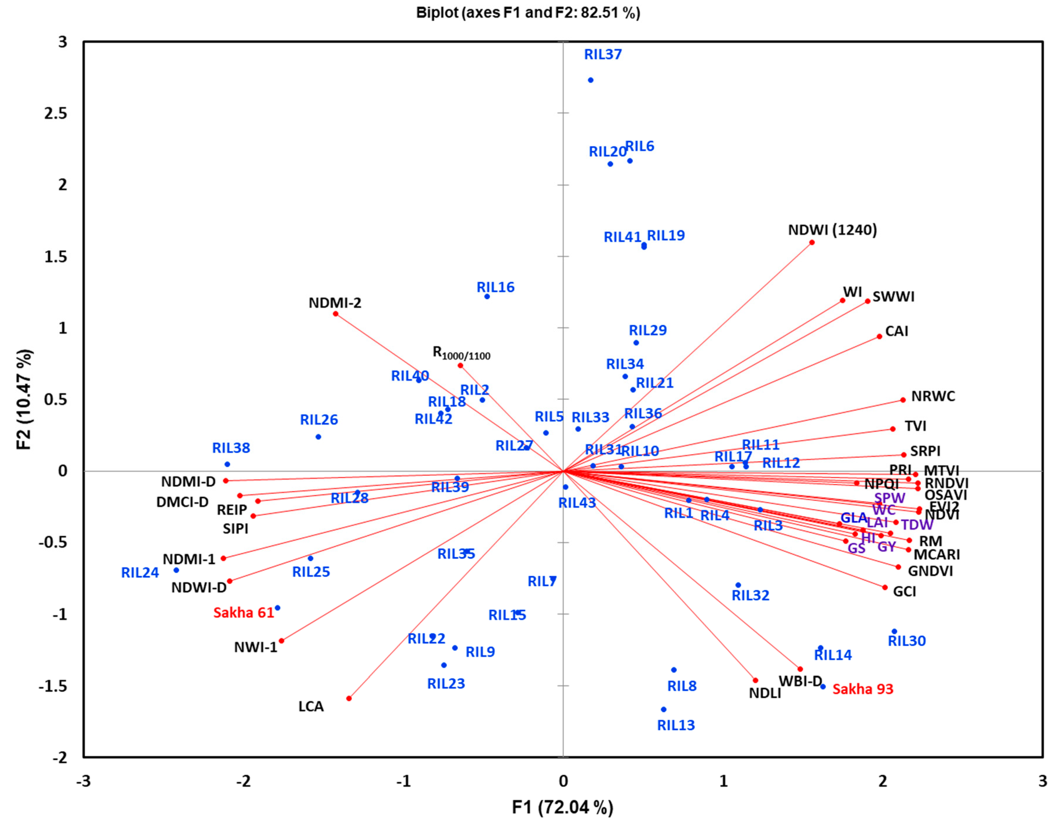
To provide a comprehensive picture of the interrelationships between all destructively measured traits, SRIs, and tested genotypes, a PCA was used to visualize this interrelationship. The results of the PCA showed that the vegetation-SRIs (except REIP and SIPI), seven out of 15 water-SRIs, and all destructively measured traits were grouped together with an acute angle between vectors (the angles between the vectors of these traits were less than 90°). However, the remaining water-SRIs and REIP and SIPI were grouped together, with an angle higher than 90° between the vectors of these SRIs and those of the destructively measured traits (Figure 2). Generally, the acute angle between the vectors of SRIs and the destructively measured traits indicated that these SRIs were strongly and positively associated with the measured traits and were able to estimate these traits indirectly. Therefore, such SRIs can be used as alternative indirect selection/breeding tools in plant breeding trials. Conversely, the angle higher than 90° between the SRIs vectors and the measured traits indicated that these SRIs exhibited negative associations with the measured traits and may be used as complementary selection tools with others SRIs in plant breeding trials. Interestingly, all destructively measured traits and most vegetation-SRIs identified the drought-tolerant parent Sakha 93 and the RILs with higher values for the measured traits. Conversely, the drought-sensitive parent Sakah 61 and RILs that exhibited low values for the measured traits were favored by most water-SRIs. Therefore, the PCA also confirmed that different SRIs could be incorporated as rapid, non-destructive, cost-efficient, and indirect tools in wheat breeding programs during the selection process.

4.2. Multivariate Statistical Analysis to Predict the Different Destructively Measured Traits

Each SRI focuses on only two–three sensitive wavelengths, which makes some SRIs highly sensitive to biomass saturation, soil background, and growth conditions effects. Therefore, different PLSR models based on full-spectrum wavelengths, multiple SRIs, or combined SRIs and destructively measured traits have been considered to increase the accuracy of estimating relevant measured traits [9,12,22,41,78,89]. For example, ElSayed et al. [22] reported that the accuracy of GY and canopy water content estimation under water stress conditions was increased when various SRIs were used simultaneously for PLSR models. Li et al. [12] also reported that incorporating the most significant SRIs (chosen via variable importance in projection) in the PLSR model increased the efficiency of LAI estimation. In addition, Yue et al. [27] found that a PLSR model based on 54 various SRIs provided the highest accuracy in leave-one-out cross-validation for estimation of the above-ground biomass of winter wheat. In the present study, when all SRIs were combined into a single dataset in PLSR to estimate different measured traits, the results showed that the PLSR models exhibited a high to moderate R² in both calibration (Cal.) and validation (Val.) datasets (R² ranged from 0.53 to 0.75 in Cal. and from 0.46 to 0.72 in Val.) (Table 5). In addition, it provided a good relationship between observed and predicted values for the measured traits (Figure 3), whereas the range of R² values and the degree of accuracy between the observed and predicted values were strongly dependent on the measured traits and season. These findings indicated that PLSR models based on various SRIs may be used to estimate indirectly the GY and different intermediate traits used widely as direct screening criteria in breeding programs aiming to improve the drought tolerance of wheat genotypes in a fast and nondestructive manner. The ability of such PLSR models to estimate indirectly destructively measured traits may be related to their ability to minimize the effects of vegetation structure, the biophysical properties of plants, soil background, and atmospheric conditions because they include a wide range of sensitive wavelengths, which are directly related to the main changes in the target traits.

To identify the most influential SRIs that explained the most variability in each destructively measured trait across genotypes, all SRIs were further applied to SMLR analysis as independent variables. Interestingly, the results of this study showed that, in general, SMLR performed better than PLSR in the estimation of measured traits, especially GLA, WC, Gs, and HI (R² values are compared in Table 5 and Table 6). In addition, the SMLR model identified NDVI, GNDVI, NPQ, and MCARI from vegetation-SRIs and NDWI₁₂₄₀, DMCI-D, and NDLI from water-SRIs as the most influential SRIs that explained much of the variation in measured traits among genotypes (explaining 0.63–0.86 of the total variability in the measured traits; Table 6). The high variability in GLA, TDW, LAI, and HI was explained by the indices belonging to vegetation-SRIs only, while the combined indices from the vegetation-SRIs and water-SRIs were the best to explain the variability in other traits (GY, SPW, WC, and Gs) (Table 6). This indicated that the vegetation-SRIs, which combined information from blue, green, and red-edge regions and were related to the leaf chlorophyll and associated pigments contents, as well as photosynthetic efficiency, were suitable for monitoring the similar vegetation related traits within the crop canopy. Conversely, the indices from water-SRIs, which combined information from NIR and SWIR regions, could be used as complementary indices to vegetation-SRIs to assess the plant traits related to changes in plant water status, internal leaf structure, and leaf biochemical compounds successfully. Previous studies have also reported that SRIs combining information from blue, green, red, and red-edge wavebands are the most effective for phenotyping several vegetation parameters, such as above-ground biomass, LAI, GLA, and other morphological traits related to growth status [9,12,78,90,91]. Conversely, those combining information from NIR and SWIR wavebands are effective for indirectly estimating GY, WC, and different plant physiological characteristics [24,87,92,93,94].

5. Conclusions

This study provides further support for the use of SRIs, for which data can be collected rapidly and cost effectively, as alternative selection tools to destructive GY and intermediate traits for enhancing the drought tolerance of spring wheat grown under limited irrigation conditions. The performance of SRIs for indirect assessment of the destructively measured traits was also evaluated using PLSR and SMLR models. The results allowed the following conclusions:

• The results of genetic analysis for destructively measured intermediate traits indicated that these traits could be used as direct traits to improve wheat production under water shortage conditions.
• Based on the genetic basis for the different SRIs, it seemed probable that rapid genetic progress could be obtained through the use of several SRIs as indirect alternative breeding/selection tools for destructively measured intermediate traits in plant breeding trials.
• The PLSR models based on all SRIs as a single index could be used for assessing the different intermediate traits that are used widely as direct screening criteria in plant breeding programs aiming to improve the drought tolerance of wheat genotypes.
• The SMLR model identified NDVI, GNDVI, NPQ, and MCARI from vegetation-SRIs and NDWI₁₂₄₀, DMCI-D, and NDLI from water-SRIs as the most influential SRIs that explained the most variability in the different destructively measured traits among genotypes.
• Based on all genetic parameters and multivariate analysis, the different SRIs could be incorporated into wheat breeding programs as effective indirect selection tools to enhance the genetic gains of drought tolerance in spring wheat.

References

1. Fereres, F.; Soriano, M.A. Deficit irrigation for reducing agricultural water use. J. Exp. Bot. 2007, 58, 147–159. [Google Scholar] [CrossRef] [PubMed] [Green Version]
2. El-Hendawy, S.E.; Schmidhalter, U. Optimal coupling combinations between irrigation frequency and rate for drip-irrigated maize grown on sandy soil. Agric. Water Manage. 2010, 97, 439–448. [Google Scholar] [CrossRef]
3. Houle, D.; Govindaraju, D.R.; Omholt, S. Phenomics: the next challenge. Nat. Rev. Genet. 2010, 11, 855–866. [Google Scholar] [CrossRef] [PubMed]
4. El-Hendawy, S.E.; Al-Suhaibani, N.; Al-Gaadi, K.; Ur Rehman, S. Capability of multiple selection criteria to evaluate contrasting spring wheat germplasms under arid conditions. Pak. J. Bot. 2015, 47, 2093–2105. [Google Scholar]
5. Lobos, G.A.; Escobar-Opazo, A.; Estrada, F.; Romero-Bravo, S.; Garriga, M.; del Pozo, A.; Poblete-Echeverría, C.; Gonzalez-Talice, J.; González-Martinez, L.; Caligari, P. Spectral reflectance modeling by wavelength selection: studying the scope for blueberry physiological breeding under contrasting water supply and heat conditions. Remote Sens. 2019, 11, 329. [Google Scholar] [CrossRef] [Green Version]
6. Sanad, M.N.M.E.; Smertenko, A.; Garland-Campbell, K.A. Differential dynamic changes of reduced trait model for analyzing the plastic response to drought phases: A case study in spring wheat. Front. Plant Sci. 2019, 10, 504. [Google Scholar] [CrossRef]
7. Lobos, G.A.; Camargo, A.; del Pozo, A.; Araus, J.L.; Ortiz, R.; Doonan, J.H. Editorial: Plant phenotyping and phenomics for plant breeding. Front. Plant Sci. 2017, 8, 2181. [Google Scholar] [CrossRef] [Green Version]
8. Potgieter, A.B.; George-Jaeggli, B.; Chapman, S.C.; Laws, K.; Suárez Cadavid, L.A.; Wixted, J.; Wason, J.; Eldridge, M.; Jordan, D.R.; Hammer, G.L. Multi-spectral imaging from an unmanned aerial vehicle enables the assessment of seasonal leaf area dynamics of sorghum breeding lines. Front. Plant Sci. 2017, 8, 1532. [Google Scholar] [CrossRef]
9. El-Hendawy, S.E.; Alotaibi, M.; Al-Suhaibani, N.; Al-Gaadi, K.; Hassan, W.; Dewir, Y.H.; Emam, M.A.E.-G.; Elsayed, S.; Schmidhalter, U. Comparative performance of spectral reflectance indices and multivariate modeling for assessing agronomic parameters in advanced spring wheat lines under two contrasting irrigation regimes. Front. Plant Sci. 2019a, 10, 1537. [Google Scholar] [CrossRef]
10. Furbank, R.T.; Jimenez-Berni, J.A.; George-Jaeggli, B.; Potgieter, A.B.; Deery, D.M. Field crop phenomics: enabling breeding for radiation use efficiency and biomass in cereal crops. New Phytol. 2019, 223, 1714–1727. [Google Scholar] [CrossRef] [Green Version]
11. Fu, Y.; Yang, G.; Wang, J.; Song, X.; Feng, H. Winter wheat biomass estimation based on spectral indices, band depth analysis and partial least squares regression using hyperspectral measurements. Comput. Electron. Agric. 2014, 100, 51–59. [Google Scholar] [CrossRef]
12. Li, X.; Zhang, Y.; Bao, Y.; Luo, J.; Jin, X.; Xu, X.; Song, X.; Yang, G. Exploring the best hyperspectral features for LAI estimation using partial least squares regression. Remote Sens. 2014, 6, 6221–6241. [Google Scholar] [CrossRef] [Green Version]
13. Atzberger, C.; Darvishzadeh, R.; Immitzer, M.; Schlerf, M.; Skidmore, A.; le Maire, G. Comparative analysis of different retrieval methods for mapping grassland leaf area index using airborne imaging spectroscopy. Int. J. Appl. Earth Obs. Geoinf. 2015, 43, 19–31. [Google Scholar] [CrossRef] [Green Version]
14. Graeff, S.; Claupein, W. Identification and discrimination of water stress in wheat leaves (Triticum aestivum L.) by means of reflectance measurements. Irrigation Sci. 2007, 26, 61–70. [Google Scholar]
15. Tilling, A.K.; O’Leary, G.J.; Ferwerda, J.G.; Jones, S.D.; Fitzgerald, G.J.; Rodriquez, D.; Belford, R. Remote sensing of nitrogen and water stress in wheat. Field Crops Res. 2007, 104, 77–85. [Google Scholar] [CrossRef]
16. Winterhalter, L.; Mistele, B.; Jampatong, S.; Schmidhalter, U. High throughput phenotyping of canopy water mass and canopy temperature in well-watered and drought stressed tropical maize hybrids in the vegetative stage. Eur. J. Agron. 2011, 35, 22–32. [Google Scholar] [CrossRef]
17. Cochavi, A.; Rapaport, T.; Gendler, T.; Karnieli, A.; Eizenberg, H.; Rachmilevitch, S.; Ephrath, J.E. Recognition of Orobanche cumana below-ground parasitism through physiological and hyperspectral measurements in sunflower (Helianthus annuus L.). Front. Plant Sci. 2017, 8, 909. [Google Scholar] [CrossRef] [Green Version]
18. Cheng, T.; Rivard, B.; Sánchez-Azofeifa, A. Spectroscopic determination of leaf water content using continuous wavelet analysis. Remote Sens. Environ. 2010, 115, 659–670. [Google Scholar] [CrossRef]
19. Zhang, L.; Zhou, Z.; Zhang, G.; Meng, Y.; Chen, B.; Wang, Y. Monitoring the leaf water content and specific leaf weight of cotton (Gossypium hirsutum L.) in saline soil using leaf spectral reflectance. Eur. J. Agron. 2012, 41, 103–117. [Google Scholar] [CrossRef]
20. Yao, X.; Jia, W.; Si, H.; Guo, Z.; Tian, Y.; Liu, X.; Cao, W.; Zhu, Y. Exploring novel bands and key index for evaluating leaf equivalent water thickness in wheat using hyperspectra influenced by nitrogen. PLoS ONE 2014, 9, e96352. [Google Scholar] [CrossRef]
21. Bayat, B.; van der Tol, C.; Verhoef, W. Remote sensing of grass response to drought stress using spectroscopic techniques and canopy reflectance model inversion. Remote Sens. 2016, 8, 557–581. [Google Scholar] [CrossRef] [Green Version]
22. Elsayed, S.; Elhewity, M.; Ibrahim, H.H.; Dewir, Y.H.; Migdadi, H.M.; Schmidhalter, U. Thermal imaging and passive reflectance sensing to estimate the water status and grain yield of wheat under different irrigation regimes. Agric. Water Manage. 2017, 189, 98–110. [Google Scholar] [CrossRef]
23. El-Hendawy, S.E.; Al-Suhaibani, N.; Elsayed, S.; Hassan, W.M.; Dewir, Y.H.; Refay, Y.; Abdella, K.A. Potential of the existing and novel spectral reflectance indices for estimating the leaf water status and grain yield of spring wheat exposed to different irrigation rates. Agric. Water Manage. 2019b, 217, 356–373. [Google Scholar] [CrossRef]
24. Prasad, B.; Carver, B.F.; Stone, M.L.; Babar, M.A.; Raun, W.R.; Klatt, A.R. Genetic analysis of indirect selection for winter wheat grain yield using spectral reflectance indices. Crop Sci. 2007, 47, 1416–1425. [Google Scholar] [CrossRef] [Green Version]
25. Erdle, K.; Mistele, B.; Schmidhalter, U. Spectral high-throughput assessments of phenotypic differences in biomass and nitrogen partitioning during grain filling of wheat under high yielding Western European conditions. Field Crops Res. 2013, 141, 16–26. [Google Scholar] [CrossRef]
26. Lobos, G.A.; Poblete-Echeverría, C.; Ahumada, L.; Zúñiga, M.; Romero, S.; Escobar, A.; Caligari, P.D.S. Fast and non-destructive prediction of gas exchange in olive orchards (Olea europaea L.) under different soil water conditions. Acta Hortic. 2014, 1057, 329–334. [Google Scholar]
27. Yue, J.; Feng, H.; Yang, G.; Li, Z. A Comparison of regression techniques for estimation of above-ground winter wheat biomass using near-surface spectroscopy. Remote Sens. 2018, 10, 66. [Google Scholar] [CrossRef] [Green Version]
28. Garriga, M.; Romero-Bravo, S.; Estrada, F.; Escobar, A.; Matus, I.A.; del Pozo, A.; Astudillo, C.A.; Lobos, G.A. Assessing wheat traits by spectral reflectance: do we really need to focus on predicted trait-values or directly identify the elite genotypes group? Front. Plant Sci. 2017, 8, 280. [Google Scholar] [CrossRef] [Green Version]
29. Kawamura, K.; Ikeura, H.; Phongchanmaixay, S.; Khanthavong, P. Canopy hyperspectral sensing of paddy fields at the booting stage and PLS regression can assess grain yield. Remote Sens. 2018, 10, 1249. [Google Scholar] [CrossRef] [Green Version]
30. El-Hendawy, S.E.; Al-Suhaibani, N.; Elsayed, S.; Refay, Y.; Alotaibi, M.; Dewir, Y.H.; Hassan, W.M.; Schmidhalter, U. Combining biophysical parameters, spectral indices and multivariate hyperspectral models for estimating yield and water productivity of spring wheat across different agronomic practices. PloS ONE 2019c, 14, e0212294. [Google Scholar] [CrossRef] [Green Version]
31. Rondeaux, G.; Steven, M.; Baret, F. Optimization of soil-adjusted vegetation indices. Remote Sens. Environ. 1996, 55, 95–107. [Google Scholar] [CrossRef]
32. Jiang, Z.; Huete, A.R.; Didan, K.; Miura, T. Development of a two-band enhanced vegetation index without a blue band. Remote Sens. Environ. 2008, 112, 3833–3845. [Google Scholar] [CrossRef]
33. Haboudane, D.; Miller, J.R.; Pattey, E.; Zarco-Tejada, P.J.; Strachan, I.B. Hyperspectral vegetation indices and novel algorithms for predicting green LAI of crop canopies: Modeling and validation in the context of precision agriculture. Remote Sens. Environ. 2004, 90, 337–352. [Google Scholar] [CrossRef]
34. Wu, C.; Niu, Z.; Tang, Q.; Huang, W. Estimating chlorophyll content from hyperspectral vegetation indices: Modeling and validation. Agric. For. Meteorol. 2008, 148, 1230–1241. [Google Scholar] [CrossRef]
35. Babar, M.A.; van Ginkel, M.; Reynolds, M.P.; Prasad, B.; Klatt, A.R. Heritability, correlated response, and indirect selection involving spectral reflectance indices and grain yield in wheat. Aust. J. Agric. Res. 2007, 58, 432–442. [Google Scholar] [CrossRef]
36. Gutierrez, M.; Reynolds, M.P.; Raun, W.R.; Stone, M.L.; Klatt, A.R. Spectral water indices for assessing yield in elite bread wheat genotypes in well irrigated, water stressed, and high temperature conditions. Crop Sci. 2010, 50, 197–214. [Google Scholar] [CrossRef]
37. Li, F.; Mistele, B.; Hu, Y.; Chen, X.; Schmidhalter, U. Reflectance estimation of canopy nitrogen content in winter wheat using optimized hyperspectral spectral indices and partial least squares regression. Euro. J. Agron. 2014, 52, 198–209. [Google Scholar] [CrossRef]
38. Elsayed, S.; Rischbeck, P.; Schmidhalter, U. Comparing the performance of active and passive reflectance sensors to assess the normalized relative canopy temperature and grain yield of drought-stressed barley cultivars. Field Crops Res. 2015, 177, 148–160. [Google Scholar] [CrossRef]
39. Hernandez, J.; Lobos, G.A.; Matus, I.; del Pozo, A.; Silva, P.; Galleguillos, M. Using ridge regression models to estimate grain yield from field spectral data in bread wheat (Triticum aestivum L.) grown under three water regimes. Remote Sens. 2015, 7, 2109–2126. [Google Scholar] [CrossRef] [Green Version]
40. Rischbeck, P.; Elsayed, S.; Mistele, B.; Barmeier, G.; Heil, K.; Schmidhalter, U. Data fusion of spectral, thermal and canopy height parameters for improved yield prediction of drought stressed spring barley. Euro. J. Agron. 2016, 78, 44–59. [Google Scholar] [CrossRef]
41. Feng, M.; Guo, X.; Wang, C.; Yang, W.; Shi, C.; Ding, G.; Zhang, X.; Xiao, L.; Zhang, M.; Song, X. Monitoring and evaluation in freeze stress of winter wheat (Triticum aestivum L.) through canopy hyper-spectrum reflectance and multiple statistical analysis. Ecol. Indicat. 2018, 84, 290–297. [Google Scholar] [CrossRef]
42. Allen, R.; Pereira, L.; Raes, D.; Smith, M. Crop Evapotranspiration. Guidelines for Computing Crop Water Requirements; FAO Irrigation and Drainage: Rome, Italy, 1998; 300p. [Google Scholar]
43. Zadoks, J.C.; Chang, T.T.; Konzak, C.F. A decimal code for the growth stages of cereals. Weeds Res. 1974, 14, 412–415. [Google Scholar] [CrossRef]
44. Gitelson, A.; Merzlyak, M.N. Spectral reflectance changes associated with autumn senescence of Aesculus hippocastanum L. and Acer platanoides L. leaves. Spectral features and relation to chlorophyll estimation. J. Plant Physiol. 1994, 143, 286–292. [Google Scholar] [CrossRef]
45. Gitelson, A.A.; Kaufman, Y.J.; Merzlyak, M.N. Use of a green channel in remote sensing of global vegetation from EOS-MODIS. Remote Sens. Environ. 1996, 58, 289–298. [Google Scholar] [CrossRef]
46. Raun, W.R.; Solie, J.B.; Johnson, G.V.; Stone, M.L.; Lukina, E.V.; Thomson, W.E.; Schepers, J.S. In-season prediction of potential grain yield in winter wheat using canopy reflectance. Agron. J. 2001, 93, 131–138. [Google Scholar] [CrossRef] [Green Version]
47. Gamon, J.A.; Peñuelas, J.; Field, C.B. A narrow-waveband spectral index that tracks diurnal changes in photosynthetic efficiency. Remote Sens. Environ. 1992, 41, 35–44. [Google Scholar] [CrossRef]
48. Gitelson, A.A.; Vina, A.; Ciganda, V.; Rundquist, D.C.; Arkebauer, T.J. Remote estimation of canopy chlorophyll content in crops. Geophys. Res. Lett. 2005, 32. [Google Scholar] [CrossRef] [Green Version]
49. Barnes, J.D.; Balaguer, L.; Manrique, E.; Elvira, S.; Davison, A.W. A reappraisal of the use of DMSO for the extraction and determination of chlorophylls a and b in lichens and higher plants. Environ. Exp. Bot. 1992, 32, 85–100. [Google Scholar] [CrossRef]
50. Peñuelas, J.; Baret, F.; Filella, I. Semi-empirical indices to assess carotenoids/chlorophyll a ratio from leaf spectral reflectance. Photosynthetica 1995, 31, 221–230. [Google Scholar]
51. Daughtry, C.S.T.; Walthall, C.L.; Kim, M.S.; De Colstoun, E.B.; McMurtrey, J.E. Estimating corn leaf chlorophyll concentration from leaf and canopy reflectance. Remote Sens. Environ. 2000, 74, 229–239. [Google Scholar] [CrossRef]
52. Broge, N.H.; Leblanc, E. Comparing prediction power and stability of broadband and hyperspectral vegetation indices for estimation of green leaf area index and canopy chlorophyll density. Remote Sens. Environ. 2001, 76, 156–172. [Google Scholar] [CrossRef]
53. Guyot, G.; Baret, F.; Major, D. High spectral resolution: Determination of spectral shifts between the red and the near infrared. Int. Arch. Photogramm. Remote Sens. 1988, 11, 750–760. [Google Scholar]
54. Penuelas, J.; Pinol, J.; Ogaya, R.; Filella, I. Estimation of plant water concentration by the reflectance Water Index WI (R900/R970). Int. J. Remote Sens. 1997, 18, 2869–2875. [Google Scholar] [CrossRef]
55. Elsayed, M.E.S.; Mistele, B.; Schmidhalter, U. Can changes in leaf water potential be assessed spectrally? Funct. Plant Biol. 2011, 38, 523–533. [Google Scholar] [CrossRef]
56. Babar, M.A.; Reynolds, M.P.; van Ginkel, M.; Klatt, A.R.; Raun, W.R.; Stone, M.L. Spectral reflectance indices as a potential indirect selection criteria for wheat yield under irrigation. Crop Sci. 2006a, 46, 578–588. [Google Scholar] [CrossRef]
57. Lozano, F.J.; Suárez-Seoane, S.; de Luis, E. Assessment of several spectral indices derived from multi-temporal Landsat data for fire occurrence probability modeling. Remote Sens. Environ. 2007, 107, 533–544. [Google Scholar] [CrossRef]
58. Wang, L.; Qu, J.J. NMDI: A normalized multi-band drought index for monitoring soil and vegetation moisture with satellite remote sensing. Geophys. Res. Lett. 2007, 34. Available online: https://agupubs.onlinelibrary.wiley.com/doi/full/10.1029/2007GL031021 (accessed on 23 October 2007). [CrossRef]
59. El-Hendawy, S.E.; Al-Suhaibani, N.; Dewir, Y.H.; El-Sayed, S.; Alotaibi, M.; Hassan, W.M.; Refay, Y.; Tahir, M.U. Ability of modified spectral reflectance indices for estimating growth and photosynthetic efficiency of wheat under saline field conditions/agronomy9010035. Agronomy 2019d, 9, 35. [Google Scholar] [CrossRef] [Green Version]
60. Gao, B.C. NDWI—A normalized difference water index for remote sensing of vegetation liquid water from space. Remote Sens. Environ. 1996, 58, 257–266. [Google Scholar] [CrossRef]
61. Hardisky, M.A.; Klemas, V.; Smart, R.M. The influence of soil salinity, growth form, and leaf moisture on the spectral radiance of Spartina alterniflora canopies. Photogramm. Eng. Remote Sens. 1983, 49, 77–83. [Google Scholar]
62. Zhang, L.; Zhou, Z.; Zhang, G.; Meng, Y.; Chen, B.; Wang, Y. Monitoring cotton (Gossypium hirsutum L.) leaf ion content and leaf water content in saline soil with hyperspectral reflectance. Eur. J. Agron. 2014, 47, 593–610. [Google Scholar] [CrossRef]
63. Nagler, P.L.; Daughtry, C.S.T.; Goward, S.N. Plant litter and soil reflectance. Remote Sens. Environ. 2000, 71, 207–215. [Google Scholar] [CrossRef]
64. Serrano, L.; Peñuelas, J.; Ustin, S.L. Remote sensing of nitrogen and lignin in Mediterranean vegetation from AVIRIS data: Decomposing biochemical from structural signals. Remote Sens. Environ. 2002, 81, 355–364. [Google Scholar] [CrossRef]
65. Daughtry, C.S.T.; Hunt, E.R.; Doraiswamy, P.C.; McMurtrey, J.E. Remote sensing the spatial distribution of crop residues. Agron. J. 2005, 97, 864–871. [Google Scholar] [CrossRef]
66. Singh, R.K.; Chaudhary, B.D. Biometrical Methods in Quantitative Genetic Analysis; Kalyani publication: New Delhi, India, 1979; p. 120. [Google Scholar]
67. Fehr, W. Principle of Cultivar Development. Theory and Technique; MacMillan Pub. Co.: New York, NY, USA, 1987; Volume I. [Google Scholar]
68. Wold, S.; Sjöström, M.; Eriksson, L. PLS-regression: A basic tool of chemometrics. Chemom. Intell. Lab. Syst. 2001, 58, 109–130. [Google Scholar] [CrossRef]
69. Haenlein, M.; Kaplan, A.M. A beginner’s guide to partial least squares analysis. Underst. Stat. 2004, 3, 283–297. [Google Scholar] [CrossRef]
70. Chen, S.; Hong, X.; Harris, C.J.; Sharkey, P.M. Sparse modeling using orthogonal forward regression with PRESS statistic and regularization. IEEE Trans. Syst. Man Cybernetic Part B: Cybernetics 2004, 34, 898–911. [Google Scholar] [CrossRef]
71. Venables, W.N.; Ripley, B.D. Modern Applied Statistics with S, 4th ed.; Springer: New York, NY, USA, 2002. [Google Scholar]
72. Vasques, G.M.; Grunwald, S.; Sickman, J.O. Comparison of multivariate methods for inferential modeling of soil carbon using visible/near-infrared spectra. Geoderma. 2008, 146, 14–25. [Google Scholar] [CrossRef]
73. Sorrells, M.E. Genomic selection in plants: empirical results and implications for wheat breeding BT—advances in wheat genetics: From genome to field. In Proceedings of the 12th International Wheat Genetics Symposium; Springer: Tokyo, Japan, 2015; pp. 401–409. [Google Scholar] [CrossRef] [Green Version]
74. Mathew, I.; Shimelis, H.; Mwadzingeni, L.; Zengeni, R.; Mutema, M.; Chaplot, V. Variance components and heritability of traits related to root: shoot biomass allocation and drought tolerance in wheat. Euphytica 2018, 214, 225. [Google Scholar] [CrossRef]
75. Chapman, S.C.; Edmeades, G.O. Selection improves drought tolerance in tropical maize populations. Crop Sci. 2010, 39, 1315. [Google Scholar] [CrossRef]
76. Bustos-Korts, D.; Boer, M.P.; Malosetti, M.; Chapman, S.; Chenu, K.; Zheng, B.; van Eeuwijk, F.A. Combining crop growth modeling and statistical genetic modeling to evaluate phenotyping strategies. Front. Plant Sci. 2019, 10, 1491. [Google Scholar] [CrossRef] [PubMed]
77. Lopes, M.; Reynolds, R. Stay-green in spring wheat can be determined by spectral reflectance measurements (normalized difference vegetation index) independently from phenology. J. Exp. Bot. 2012, 63, 3789–3798. [Google Scholar] [CrossRef] [PubMed] [Green Version]
78. Zerner, M.C.; Rebetzke, G.J.; Gill, G.S. Genotypic stability of weed competitive ability for bread wheat (Triticum aestivum) genotypes in multiple environments. Crop Pasture Sci. 2016, 67, 695–702. [Google Scholar] [CrossRef]
79. Walter, J.D.C.; Edwards, J.; McDonald, G.; Kuchel, H. Estimating biomass and canopy height with LiDAR for field crop breeding. Front. Plant Sci. 2019, 10, 1145. [Google Scholar] [CrossRef]
80. Acreche, M.M.; Slafer, G.A. Grain weight radiation interception and use efficiency as affected by sink-strength in Mediterranean wheat released from 1940 to 2005. Field Crops Res. 2009, 110, 98–105. [Google Scholar] [CrossRef]
81. Reynolds, M.; Foulkes, M.J.; Slafer, G.A.; Berry, P.; Parry, M.A.J.; Snape, J.W.; Angus, W.J. Raising yield potential in wheat. J. Exp. Bot. 2009, 60, 1899–1918. [Google Scholar] [CrossRef] [Green Version]
82. Medrano, H.; Escalona, J.M.; Bota, J.; Gulías, J.; Flexas, J. Regulation of photosynthesis of C3 plants in response to progressive drought: Stomatal conductance as a reference parameter. Ann. Bot. 2002, 89, 895–905. [Google Scholar] [CrossRef]
83. Flexas, J.; Bota, J.; Loreto, F.; Cornic, G.; Sharkey, T.D. Diffusive and metabolic limitations to photosynthesis under drought and salinity in C3 plants. Plant Biol. 2004, 6, 269–279. [Google Scholar] [CrossRef]
84. Falconer, D.S. Introduction to Quantitative Genetics, 3rd ed.; Longman Scientific and Technical: New York, NY, USA, 1989. [Google Scholar]
85. Trachsel, S.; Burgueno, J.; Suarez, E.A.; San Vicente, F.M.; Rodriguez, C.S.; Dhliwayo, T. Interrelations among early vigor, flowering time, physiological maturity, and grain yield in tropical maize (Zea mays L.) under multiple abiotic stresses. Crop Sci. 2017, 57, 229–242. [Google Scholar] [CrossRef]
86. Maimaitiyiming, M.; Ghulam, A.; Bozzolo, A.; Wilkins, J.L.; Kwasniewski, M.T. Early detection of plant physiological responses to different levels of water stress using reflectance spectroscopy. Remote Sens. 2017, 9, 745. [Google Scholar] [CrossRef] [Green Version]
87. Kim, D.M.; Zhang, H.; Zhou, H.; Du, T.; Wu, Q.; Mockler, T.C.; Berezin, M.Y. Highly sensitive image-derived indices of water- stressed plants using hyperspectral imaging in SWIR and histogram analysis. Sci. Rep. 2015, 5, 15919. [Google Scholar] [CrossRef] [PubMed] [Green Version]
88. Kovar, M.; Brestic, M.; Sytar, O.; Barek, V.; Hauptvogel, P.; Zivcak, M. Evaluation of hyperspectral reflectance parameters to assess the leaf water content in soybean. Water 2019, 11, 443. [Google Scholar] [CrossRef] [Green Version]
89. Christenson, B.S.; Schapaugh, W.T.; Nan, J.R.; Price, K.P.; Prasad, V.; Fritz, A.K. Predicting soybean relative maturity and seed yield using canopy reflectance. Crop Sci. 2016, 56, 625–643. [Google Scholar] [CrossRef] [Green Version]
90. Delegido, J.; Verrelst, J.; Meza, C.M.; Rivera, J.P.; Alonso, L.; Moreno, J. A red-edge spectral index for remote sensing estimation of green LAI over agro-ecosystems. Eur. J. Agron. 2013, 46, 42–52. [Google Scholar] [CrossRef]
91. Babar, M.A.; Reynolds, M.P.; van Ginkel, M.; Klatt, A.R.; Raun, W.R.; Stone, M.L. Spectral reflectance to estimate genetic variation for in-season biomass, leaf chlorophyll, and canopy temperature in wheat. Crop Sci. 2006, 46, 1046–1057. [Google Scholar] [CrossRef]
92. Romero, A.; Aguado, I.; Yebra, M. Estimation of dry matter content in leaves using normalized indexes and PROSPECT model inversion. Int. J. Remote Sens. 2012, 33, 396–414. [Google Scholar] [CrossRef]
93. Rapaport, T.; Hochberg, U.; Cochavi, A.; Karnieli, A.; Rachmilevitch, S. The potential of the spectral ‘water balance index’ (WABI) for crop irrigation scheduling. New Phytolog. 2017, 216, 741–757. [Google Scholar] [CrossRef] [Green Version]
94. Wang, C.; Feng, M.; Yang, W.; Ding, G.; Xiao, L.; Li, G.; Liu, T. Extraction of sensitive bands for monitoring the winter wheat (Triticum aestivum) growth status and yields based on the spectral reflectance. PloS ONE 2017, 12, e0167679. [Google Scholar] [CrossRef]
Figure 1. Correlation matrix between different destructively measured traits and spectral reflectance indices across genotypes and seasons (n = 90). GY, grain yield; GLA, green leaf area; TDW, total dry weight; WC, water content; SPW, spike weight; HI, harvest index.
Remotesensing 12 01480 g001
Figure 2. Biplot of the principle component analysis for the first two principle components of all destructively measured traits, spectral reflectance indices, and genotypes. The data are averaged over two growing seasons.
Remotesensing 12 01480 g002
Figure 3. Linear relationship between the observed and predicted values of different destructively measured traits under the first and second season. Predicted values were derived from partial least squares regressions using all spectral reflectance indices for genotypes and two seasons (n = 45).
Remotesensing 12 01480 g003