Abstract
The persistence and productivity of forage grasses, important sources for feed production, are threatened by climate change-induced drought. Breeding programs are in search of new drought tolerant forage grass varieties, but those programs still rely on time-consuming and less consistent visual scoring by breeders. In this study, we evaluate whether Unmanned Aerial Vehicle (UAV) based remote sensing can complement or replace this visual breeder score. A field experiment was set up to test the drought tolerance of genotypes from three common forage types of two different species: Festuca arundinacea, diploid Lolium perenne and tetraploid Lolium perenne. Drought stress was imposed by using mobile rainout shelters. UAV flights with RGB and thermal sensors were conducted at five time points during the experiment. Visual-based indices from different colour spaces were selected that were closely correlated to the breeder score. Furthermore, several indices, in particular H and NDLab, from the HSV (Hue Saturation Value) and CIELab (Commission Internationale de l’éclairage) colour space, respectively, displayed a broad-sense heritability that was as high or higher than the visual breeder score, making these indices highly suited for high-throughput field phenotyping applications that can complement or even replace the breeder score. The thermal-based Crop Water Stress Index CWSI provided complementary information to visual-based indices, enabling the analysis of differences in ecophysiological mechanisms for coping with reduced water availability between species and ploidy levels. All species/types displayed variation in drought stress tolerance, which confirms that there is sufficient variation for selection within these groups of grasses. Our results confirmed the better drought tolerance potential of Festuca arundinacea, but also showed which Lolium perenne genotypes are more tolerant.
1. Introduction
Grasslands cover about 30% of the agricultural area in Europe (EU28) [1] and represent a substantial economic value through feed production. At the same time, they are also crucial for biodiversity and carbon sequestration [2,3,4]. However, grassland persistence and productivity is very sensitive to drought [5,6]. The increasing frequency and intensity of dry spells in Western Europe as a consequence of climate change substantially impacts the production and carbon sequestration capacity of these grasslands [7,8,9]. It is therefore important that new varieties of forage grasses possess a good drought tolerance as part of the adaptation strategy of the fodder production system to the changing climate [10].
In temperate regions like Western Europe, perennial ryegrass (Lolium perenne L.) and tall fescue (Festuca arundinacea Schreb.) are two of the major perennial forage grass species used for fodder production. Lolium perenne (Lp) is praised for its excellent feeding quality both for grazing and mowing. Perennial ryegrass occurs in nature as a diploid, but breeders have developed tetraploid varieties after chromosome doubling by e.g., colchicine treatment [11]. Tetraploid ryegrasses have a lower dry matter content, but this is compensated by a higher resistance to crown rust and snow mould and a higher fresh yield. In addition, tetraploid varieties have a more open sward and are less persistent [12]. Although Festuca arundinacea (Fa) has a lower feeding quality than Lp, its yield potential is larger, especially under drought conditions, owing to its deeper rooting [13,14,15].
Attaining a higher level of tolerance to drought in new cultivars of these grass species implies phenotyping for this trait across a wide range of genotypes/accessions in breeding programs. This typically requires thousands of genotypes/plants to be evaluated under water-limited conditions. To this end, drought tolerance testing is preferably done in the field and using rainout shelters, since these block the precipitation, while having a relatively limited impact on temperature rise or light level reduction [16]. In addition, the root growth of the plants is not limited in contrast with pot experiments [17].
In forage grass breeding programs in Western Europe, the early phase of the breeding program aims to select the best genotypes from a large pool of individual plants by visually assigning a score to their appearance. This breeder score is based on an evaluation of the greenness, biomass and health of the plant, and can therefore also be used for scoring drought tolerance. As this is an ‘integrative’ score, it is not possible to disentangle particular reactions and adaptations of the different genotypes to drought. Hence, these breeder scores cannot infer whether the apparent drought tolerance is the result from e.g., a deep rooting system, or from efficient stomatal behaviour. Nevertheless, this scoring allows to capture a substantial amount of variation that can be attributed to genotypic differences among the plants. The proportion of the total variation that can be attributed to genotype variation is called ‘broad-sense’ heritability, and is impacted by the experimental conditions and the observation method [18]. Scoring one single plant takes very little time, but since many plants (thousands in one experiment) need to be scored, assigning breeder scores is labour-intensive. Furthermore, factors as fatigue and changing weather conditions can result in ‘within-observer’ inconsistencies, even for highly skilled observers [19]. Furthermore, visual scores are prone to subjectivity of the observer [20], as individual criteria of observers differ slightly, and thus result in a low ‘between-observer’ consistency [19]. Because of these limitations, high throughput field phenotyping (HTFP) with close-range remote sensing, including from UAVs (Unmanned Aerial Vehicles), provides an interesting alternative [21]. The initial focus for this kind of screening was on multispectral sensors covering the visual and near infrared wavelengths [21,22], allowing the calculation of standard vegetation indices (VIs) as Normalized Difference Vegetation Index (NDVI; [23]) or Soil-Adjusted Vegetation Index (SAVI; [24]). UAV-based NDVI has already been demonstrated to be well-correlated with visual scoring by breeders for perennial ryegrass [25]. Recently, the use of commercial RGB (Red/Green/Blue) sensors receives increasing attention as low-cost and reliable alternatives [26,27,28,29], from which crop height and size or specific VIs can be derived.
Several studies even report that RGB-based remote sensing outperforms conventional multispectral remote sensing, e.g., for assessing crop growth (e.g., [30]), nutrient levels [31,32] or weed detection [26,33]. This seems particularly the case in applications where very high spatial resolution outweighs spectral resolution [26,34]. Vegetation indices that can be calculated directly from the RGB colour space include for instance Excess Green (; [35]) and Green-Red Vegetation Index (; [36,37]). In addition, the RGB information can be converted to alternative colour spaces, from which additional indices can be calculated. These other colour spaces, such as CIE (Commission Internationale de l’éclairage) Lab, CIELuv, HSV (Hue-Saturation-Value) or HSL (Hu-Saturation-Lightness), can be calculated from RGB data and were developed to more accurately represent the colours as observed by the human eye [38,39]. They are also less influenced by the specific differences in illumination and shade within and between images [40,41]. The use of different colour spaces is well-established for estimating fractional crop cover and for image segmentation and classification (e.g., [38,42,43,44,45,46,47], but has also been applied for disease detection [48] and for assessing nitrogen content of leaves and canopies [39,49].
In the context of grass breeding and phenotyping trials, previous research demonstrated the potential of UAV-based RGB data for objectively measuring persistency and biomass [19,50]. In this article, we are investigating whether visual-based indices can also be used to complement, or even replace, visual breeder scores. In this context, we hypothesize that VIs based on advanced colour spaces are better related to the breeder scores, since these are more similar to the colour perception by the human eye. When focusing on tolerance to drought, thermal imagery can be of particular importance in HTFP, as drought stress often leads to the physiological plant response of stomatal closure, and consequently leaf temperature increase [29,51,52]. Unlike RGB-based information, which typically presents an integrative result over time (e.g., growth and vegetation indices), thermal imagery provides an instantaneous readout of the plant’s ecophysiological status. UAV-based thermal imagery has been applied in phenotyping for drought stress tolerance in trees [53,54], wheat [29,55], soybean [56] and sugarcane [57].
The overall aim of this study is to evaluate the use of UAV-based remote sensing for complementing or replacing the breeder score and for assessing the drought tolerance of individual genotypes of three forage grass types, belonging to two species: tall fescue (Fa), diploid perennial ryegrass (Lp2) and tetraploid perennial ryegrass (Lp4). More specifically, we address four research questions:
- Which RGB-based indices correlate best to the breeder score for screening drought stress tolerance in forage grasses?
- Does the single-trial ‘broad-sense’ heritability (i.e., the proportion of total variance that can be attributed to genotypic variance) differ between the breeder score and these indices?
- Is there an added value of thermal imagery for screening drought stress tolerance in forage grasses?
- Can we infer distinct behaviour in response to drought stress within and between the three grass forage species/types?
2. Materials and Methods
2.1. Field Trial
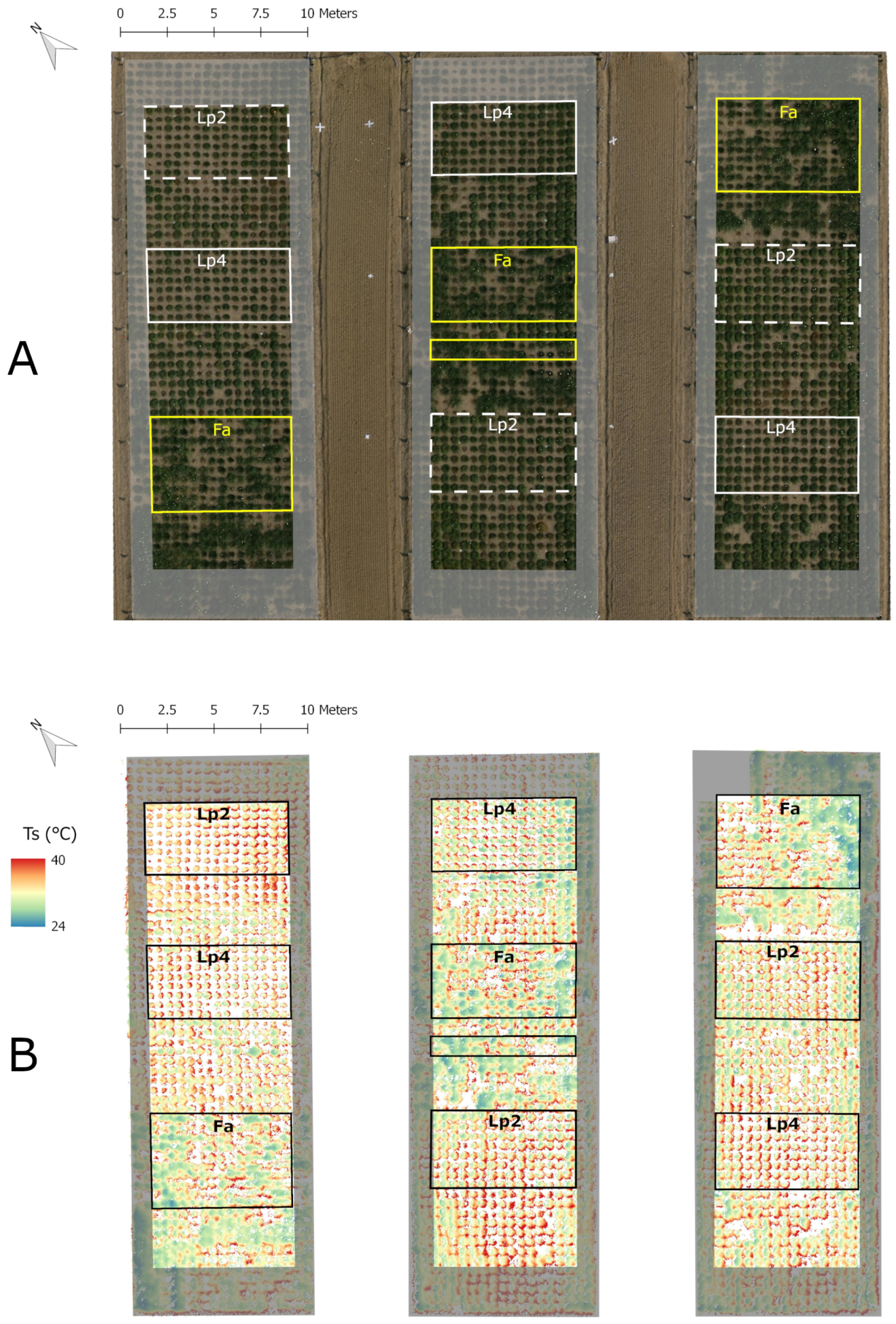
In the first half of April 2013, 150 genotypes of Festuca arundinacea Schreb. (hereafter named Fa), 120 genotypes of diploid Lolium perenne L. (hereafter named Lp2) and 120 genotypes of tetraploid Lolium perenne L. (hereafter named Lp4) were selected from the Ghent University (Fa) and the ILVO (Research Institute for Agriculture, Fisheries and Food) (Lp2, Lp4) breeding gene pool and planted as spaced plants (planting distance m × m) in a field (soil texture: sandy loam) equipped with three mobile rainout shelters at ILVO, Melle (50 59.5’ N, 3 47.1’ E) (Figure 1). Although we realize that diploid (Lp2) and tetraploid (Lp4) perennial ryegrass are not different species, for ease of interpretation we regarded them as different species in the remainder of the analysis. The experiment was organised as an alpha design with 15 blocks (), 8 to 10 genotypes per block () and three replications (, one in each rainout shelter) using the package agricolae and the function design.alpha in the RStudio software [58,59]. As such, there were 1170 plants () under evaluation (marked by the boxes in Figure 1). Besides the plants under study, 1080 other grass plants were planted (360 per rainout shelter), but these plants were not the subject of the current study. In the middle of each of the three plots, a hole (90 cm deep, 40 cm diameter) was dug, to install soil moisture sensors across a 80 cm soil profile. To avoid impact of this soil disturbance on the Fa plants under study in the middle plot, we planted non-studied plants in the two rows bordering the hole. As a result, the Fa sub-plot in the middle plot was divided into two parts Figure 1.
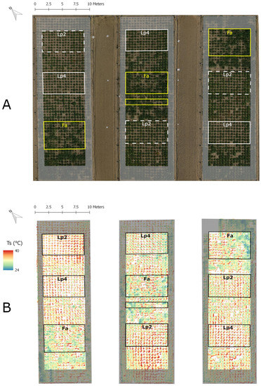
Figure 1.
Orthophoto (RGB; A) and false colour image of plant surface temperature (; B) of the experimental field on 6 September 2013 (DOY 249). The three parts of the field correspond to the three rainout shelters. Grey shaded areas include border plants, the framed areas contain the plants used for this study. In part (B) (thermal image) the soil pixels were filtered out to improve visualisation. Ts was calculated according Equation (1).
The three rainout shelters, each 30 m long and 10 m wide, are located next to each other (Figure 1). To reduce edge effects, two additional border rows were planted with individuals of the neighbouring species at the long edges of the three plots. Five rows of border plants were planted at the short edges, as these sides of the rainout shelters were more open, and thus potentially more vulnerable for sideward incoming rain (Figure 1). These five border rows also consisted of individuals of the neighbouring species.
After planting, but before the start of the drought treatment, five plants had died (three of Fa and two of Lp4), thus resulting in a total of 1165 plants under evaluation. Plants were mown on 28 May (DOY 148), 26 June (DOY 177), 30 July (DOY 211) and 24 September (DOY 267). Fertilizer was applied on 29 May (DOY 149, 53 kg N ha + 18 kg P2O5 ha + 77 kg K2O ha), on 29 June (DOY 180, 60 kg N ha + 20 kg P2O5 ha + 88 kg K2O ha), and on 30 July (DOY 211, 40 kg N ha).
2.2. Drought Treatment
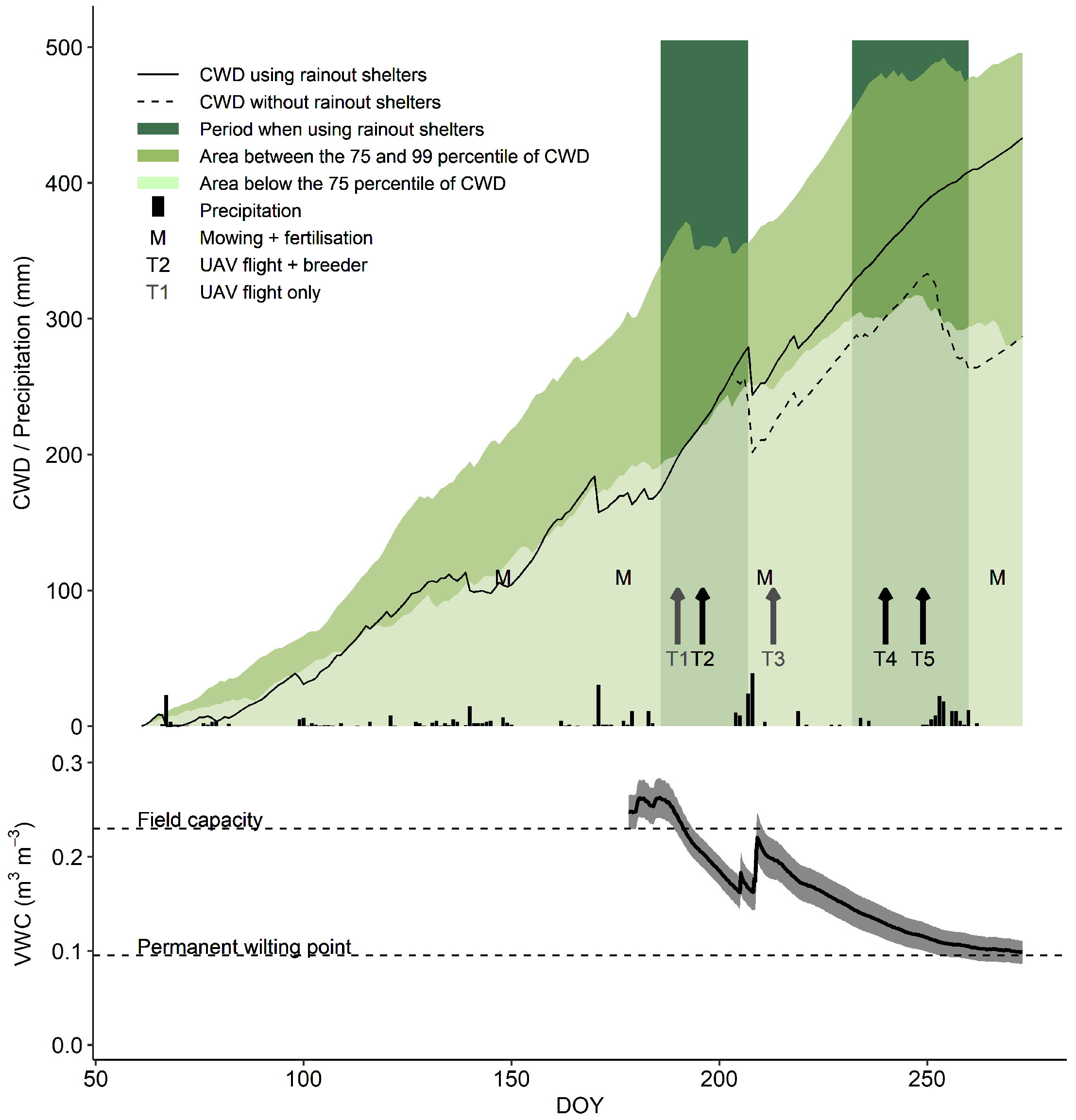
The rainout shelters were moved over the experimental field during two periods of the 2013 summer season (from DOY 186 until 207 and from DOY 232 until 260, Figure 2). In-between these two periods, plants were mown and fertilized, and were exposed to two rain events to allow the fertilizer to dissolve. Before, during and after the drought periods, meteorological conditions were recorded using a temperature + relative humidity (RH) probe (CS215, Campbell Scientific, Inc., Logan, UT, USA), a precipitation sensor (ARG100, Campbell Scientific, Inc., Logan, UT, USA) and a pyranometer (LP02, Hukseflux, The Netherlands) installed about 15 m from the experimental set-up. Furthermore, the volumetric water content of the soil (VWC in m m) was monitored continuously for the 10–40 cm depth at 6 locations per rainout shelter (18 in total) using Time Domain Reflectometry sensors (type CS616, Campbell Scientific Inc., UK) (Figure 2).
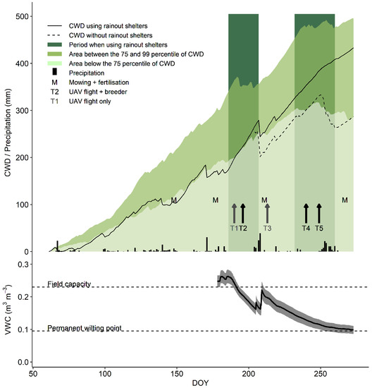
Figure 2.
Visual representation of the environmental conditions, management actions and the time points of measurements during the experiment. The upper part displays the evolution of the cumulative water deficit (CWD; (mm)), and precipitation along with the timing of rainout shelter use, mowing and fertilisation, and observations. The lower graph shows the evolution of the volumetric soil moisture content (VWC; 10 to 40 cm profile; (m m)) as an average of 18 sensors distributed over the field. The grey shaded area represents the 95% confidence interval on the data.
CWD was calculated as the accumulation of the difference between daily reference evapotranspiration (ET0 in mm) and precipitation (P in mm). ET0 was calculated using the ET.PenmanMonteith function of the R package Evapotranspiration [60,61].
2.3. Breeder Score
During the experiment, plants were scored by one experienced forage grass breeder on 16 July, 29 August and 6 September (T2, T4 an T5 resp. in Figure 2). Plant scores varied from 1 to 9 and integrate both the amount of biomass and the green colour of the plant. Higher values are assigned to plants with high biomass levels (i.e., yield) that are green and healthy-looking.
2.4. Uav-Based Remote Sensing and Image Analysis
Aerial imagery was obtained with an AT8 octocopter of AerialTronics (Scheveningen, The Netherlands), from flights carried out on five sunny days between 9 July and 6 September 2013 (Figure 2). The UAV was equipped with both a thermal and an RGB sensor, installed on a 2 axis AV2000 gimbal (PhotoHigher, Wellington, New Zealand), which had a nadir orientation for all flights. Flights were performed following a pre-programmed waypoint route of 9 parallel flight lines, at 4 m from each other, at a flight speed of 1.5 to 2 m s and at a flight height of 12–14 m. The thermal sensor, a FLIR SC305 (FLIR Systems, Inc., Wilsonville, OR, USA), had a resolution of 320 × 240 pixels, a thermal accuracy of ±2 C and a thermal sensitivity of 0.05 C , and was equipped with a 10 mm lens with a field of view (FOV) of 45 × 34. At 12 m altitude, each single image covered about 10.0 m × 7.3 m, with a resolution of 2.9 cm. An on-board computer (Olimex) was used to take images every 2 to 2.5 s, resulting in a horizontal and vertical overlap of 60%. The at-sensor radiance was converted into brightness temperature (Tbr) by using the FLIR ThermaCam Researcher Pro 2.10 software (FLIR Systems, Inc., Wilsonville, OR, USA) for performing the atmospheric correction, with the locally measured air temperature and relative humidity (Table 1), and a flight height of 12 m as input parameters [62]. Surface temperature (Ts) was then calculated as:
in which is the emissivity, estimated as 0.985, and Tbg is the background temperature, retrieved by measuring the brightness temperature of a reference panel covered with aluminium sheet [62,63].

Table 1.
Air temperature (Tair), vapour pressure deficit (VPD) and background temperature (Tbg) of the reference panels during the UAV flights.
The RGB sensor was a 12MP Canon S110 (Canon, Japan). Its spectral response (Figure S1) is typical of a consumer-grade digital RGB camera, with some overlap between the blue, green and red spectra [64,65]. It was set to the maximal field of view 74× 53 (5.2 mm focal length, 24 mm equivalent). Image parameters were set manually before each flight and remained the same for the entire flight. The sensor was programmed with CHDK (https://chdk.fandom.com/) to log every second. Individual images cover about 18.0 × 12.0 m with a spatial resolution of 0.4 cm. Horizontal overlap was 75% and vertical overlap was 88%. Georeferenced RGB and thermal orthophotos were assembled with AgiSoft PhotoScan Pro v1.2.6 (AgiSoft LLC, St-Petersburg, Russia), with GPS data extracted from the GPX-logfile of the UAV. The RGB orthophotos of 16 July served as base map to register all other RGB data and all thermal data in PhotoScan, using ground control points visible in both the base map and the other datasets. All further processing then occurred with ArcGIS 10.1 (ESRI, Redlands, CA, USA). On the flight of 1 August (T3, Figure 2), the grass plants had been recently mown, and individual plants did not overlap. The Green Chromatic Coordinate index () and Excess Green index () were calculated from the RGB image of this day, and a vegetation mask was created from these indices based on threshold values. A polygon shapefile was generated automatically from the mask, and this shapefile was checked manually to ensure that each polygon corresponded with a single grass plant. All shapefiles were negatively buffered by 5 cm to avoid edge effects or remaining inconsistencies due to imperfect image co-registration. Row and column numbers were assigned to each polygon and were used to link each plant polygon to the species and block. In total, 1165 polygons were created. For each flight day and for the RGB and surface temperature image separately, the polygons were checked visually to make sure they covered the area of the plant- if not, the polygon location was adjusted for this particular time point and sensor. An example of the polygons for different time points and for both surface temperature and RGB imagery is given in Figure S2. Next, for each time point (T1–T5, Figure 2), the median R, G and B (all in 8-bit digital numbering—so ranging between 0 and 255) and (in C ) per plant were calculated and saved, and these data served as the basis for the calculations of all vegetation indices. On T2 (16 July), because of a problem with the logger system of the thermal sensor, no thermal data were available for a full block of Lp4; for this day, the thermal data for Lp4 were not included in the analyses.
2.5. Calculation of Vegetation Indices
From the RGB data, 35 different VIs were calculated, hereafter referred to as ‘visual-based indices’, belonging to five different colour spaces (RGB, CIELab, CIELuv, HSL and HSV)—see Table 2 for a full overview. To convert the RGB data to the different colour spaces, scripts were developed in Matlab R2018b (Mathworks Inc., Natic, MA, USA) based on the formulas provided by http://www.easyrgb.com/en/math.php#text2. The HSL and HSV colour spaces are very similar, and break down the data into a colour hue (H), saturation or colour purity (S), and brightness (Value in HSV, Luminosity in HSL) [38]. The CIELab and CIELuv colour spaces are also similar. One dimension represents luminance or lightness (L*), whereas the other two dimensions represent chrominance and separate the colour spectrum. For instance, negative values of the a* dimension represent a green colour, positive values a red colour, whereas the b* dimension expresses a blue (negative) to yellow (positive) spectrum [38,39].

Table 2.
Overview of the different RGB-based vegetation indices (VIs) and their colour space used in this study.
From the thermal data, two indices (further thermal-based indices), and the Crop Water Stress Index (CWSI), were calculated as:
with being the air temperature and with and corresponding to the surface temperature of a grass plant transpiring at maximal rate () and not transpiring at all () [51,74]. In this case, and were calculated directly per measurement day as the 1st and 99th percentile of the polygon records of that day. This histogram approach is commonly applied [75,76,77] and assumes that on any given measurement day, (at least) 1% of the plants were not transpiring at all, and (at least) 1% of the plants were transpiring at potential (maximal) level. In this case, given the large number of plants and the large range in drought sensitivity among the species, we believe this is a valid assumption.
2.6. Data Analysis Workflow
On flight times T2, T4 and T5, breeder scores taken from the same or previous day were available. For those days, Pearson correlations were calculated between the different VIs and the breeder scores. Correlations were calculated for each day separately as well as for the data of the three flight days combined. In addition, correlations were calculated per species as well as for all plants together. In all cases, the correlations were calculated using the individual plant data. The adjusted mean value of each VI for each plant and for each time point was calculated taking into account the block effects of the alpha design in the mixed-effects model of the PBIB.test function of the agricolae package in R [58,59]. Using the variance analysis output of the PBIB.test function, the single-trial broad-sense heritability () for each VI at each time point (T1–T5) and for each species (Fa, Lp2, Lp4) was computed using:
where is the genotypic variance, and the total phenotypic variance. Next, a Principal Component Analysis (PCA) and a hierarchical clustering analysis was carried out on the scores per plant and per measurement day of CWSI and a selection of the visual-based VIs that were promising in terms of correlation with the breeder score and , using the PCA and HCPC functions of the FactoMineR package in R [59,78]. Based on the PCA, we selected one index per colour space and one thermal index for deeper analysis.
3. Results
3.1. Environmental Conditions
Rainout shelters were used for two periods to gradually reduce water availability in field conditions Figure 2. Near the end of the first drought treatment period, the volumetric water content for the 10–40 cm soil profile (VWC) dropped to about 0.16 m m, corresponding to 40% of relative extractable water (REW). During the second drought period, VWC dropped to levels close to the wilting point (0% REW). However, at this time (around DOY 270), deeper soil layers (50–80 cm) still had higher VWC levels (Figure S3), and potentially provided water for deeper rooting genotypes. The cumulative water deficit (CWD) resulting from these treatments was situated between the 75th and 99th percentile, based on weather data from 1975 to 2019 for Flanders.
3.2. Breeder Scores
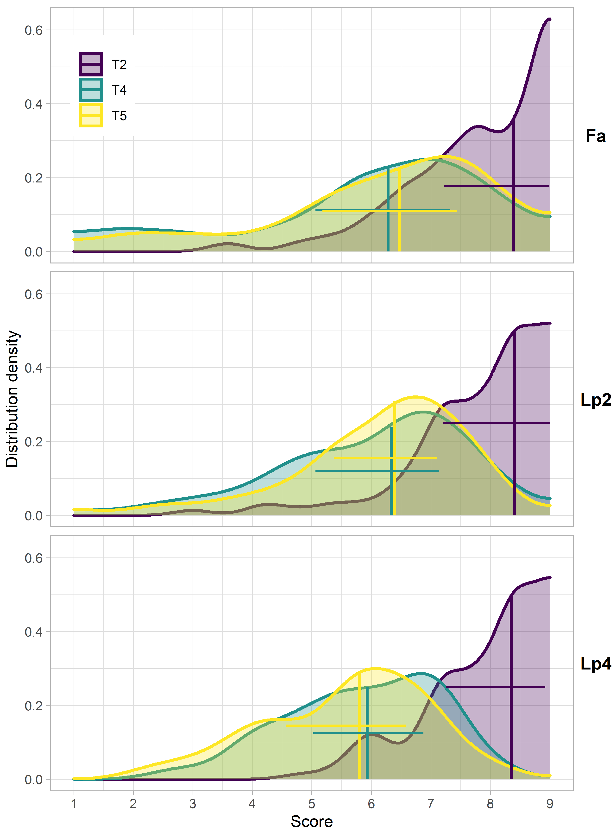
The distributions of the breeder scores showed that for all species (Fa, Lp2 and Lp4), the median values of the breeder score were highest at T2, at the start of the experiment (Figure 3). At T4 and T5, the spread on the scores increased compared to T2. At these time points (T4 and T5), the proportion of both the high scores (9) and the low scores (1) was substantially higher for Fa, compared to Lp2 and Lp4. For Fa, the median score at T5 was higher than at T4, whereas there was almost no difference between these two dates in Lp2. In Lp4 on the other hand, the median value at T5 was lower compared to T4.
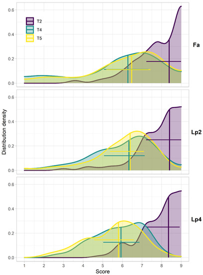
Figure 3.
Distributions of the breeder scores at the different time points (T2, T4, T5) for the different species (Fa: Festuca arundinacea; Lp2: diploid Lolium perenne; Lp4: tetraploid Lolium perenne). Data are the adjusted means calculated using the PBIB.test function of the agricolae package in R [58]. Vertical lines indicate the median, horizontal lines indicate the range between the 25th and 75th percentile.
3.3. Correlating Breeder Scores and Vegetation Indices
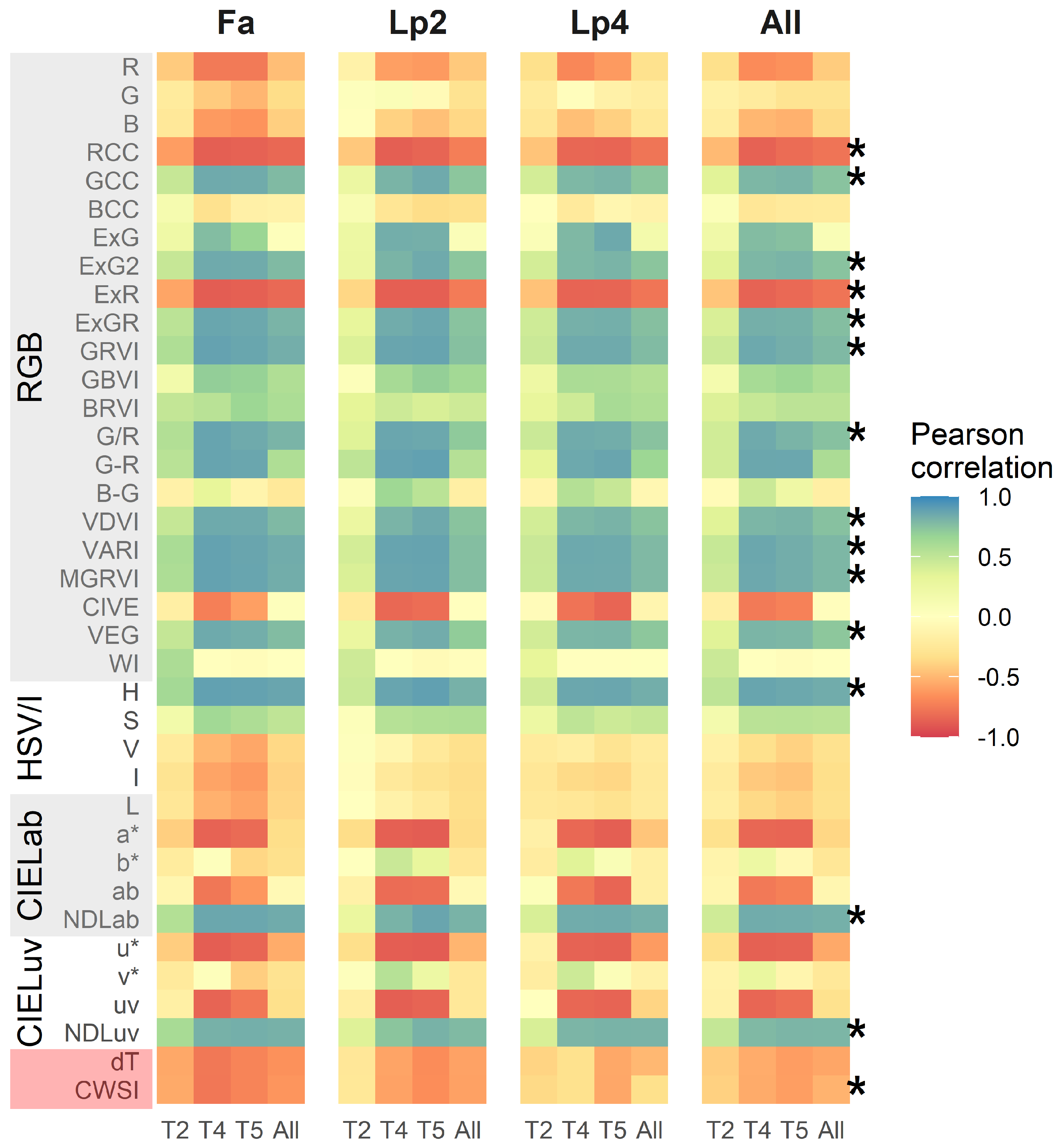
The Pearson correlation statistic between each of the 37 indices (35 visual-based and 2 thermal) and the breeder score is given in Figure 4, for each species separately and for all species together as well as for the three time points (T2, T4 and T5) separately and all time points together. In general, correlations between the breeder scores and the VIs were lower at T2 than at T4 and T5. For the visual-based indices, there was no clear species effect on the linear regressions between indices and the breeder score, resulting in a similar correlation when all species were taken together (Panel “All” in Figure 4). However, for some indices (ExG, G-R, CIVE, a*, ab, u* and uv), there was a good correlation with the breeder score for each single time point, even across the species, but this correlation was substantially lower when all time points were pooled. For these overall data, the VIs with the highest correlations with the breeder score were H (r = 0.84), NDLab (r = 0.82), MGRVI (r = 0.79) and VARI (r = 0.79). Correlations between the breeder scores and the thermal indices ( and CWSI) were considerably lower than for the best-performing visual-based indices, and were stronger for Fa than for Lp2 and Lp4.
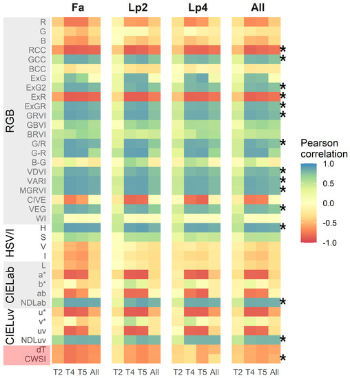
Figure 4.
Pearson correlations between 37 different indices and the breeder score per species separately (Fa: Festuca arundinacea; Lp2: diploid Lolium perenne; Lp4: tetraploid Lolium perenne) and all species together (All) and per time point (T2, T4 and T5) and all time points together (All). The different indices are organized by sensor and colour space. Asterisks (*) point out indices of which the overall correlation was above 0.70 or below −0.70 and which were used for further analyses, along with CWSI.
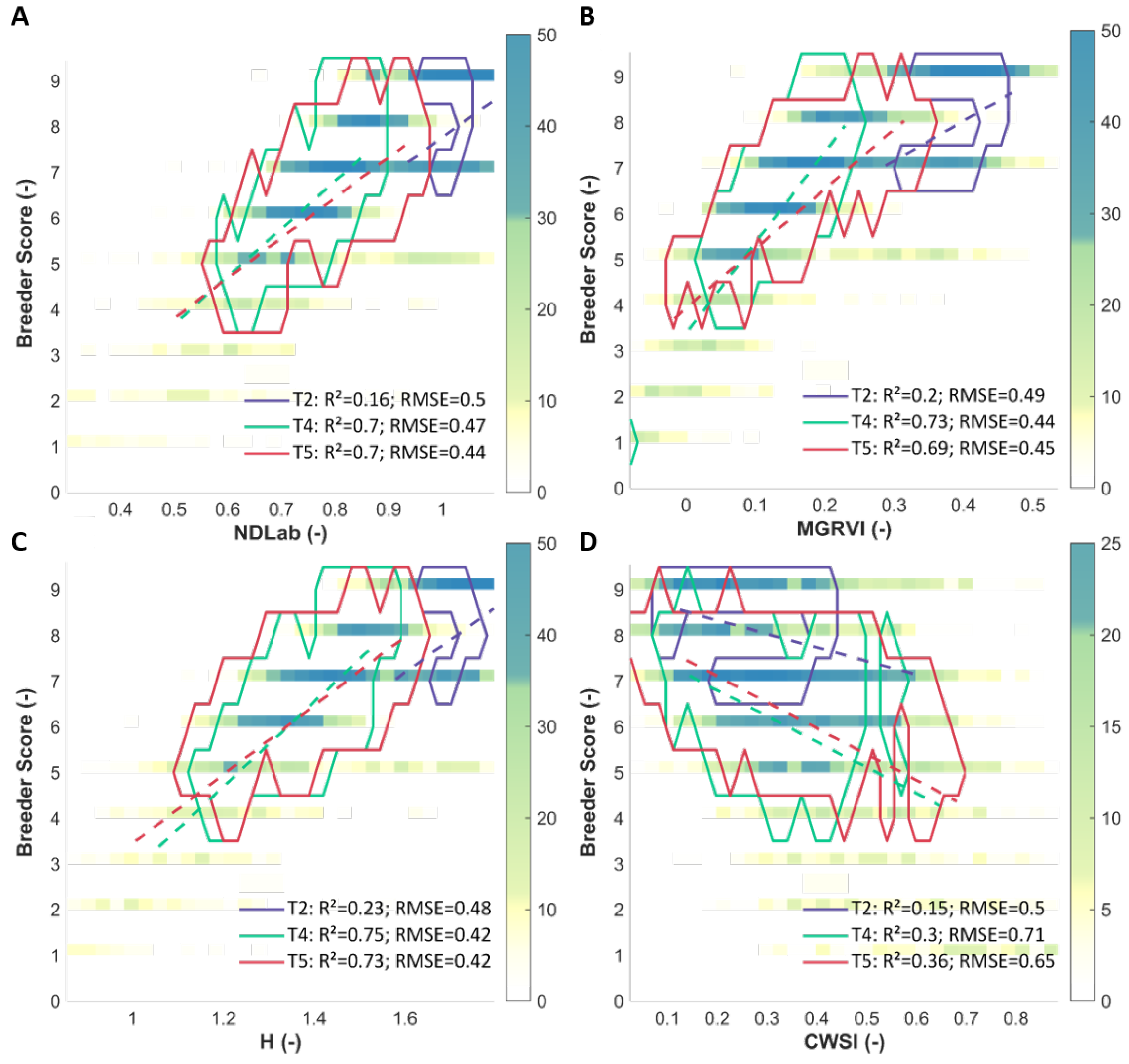
We selected the indices with a correlation value above 0.7 or below −0.7 across all time points and species, as well as the thermal based CWSI, for further analysis. These selected indices are marked with an asterisk in Figure 4. The relations of the breeder score with MGRVI, H, NDLab and CWSI as a function of time are visualised in Figure 5. These density plots indicate that the spread on the data was smallest at T2, whereas T4 and T5 displayed more variation and showed a clearer correlation between UAV-based indices and the breeder score.

Figure 5.
Density plots of H, NDLab, MGRVI, and CWSI (panels A–D) versus the breeder score, with linear regression (dashed line) and contour plot (full) per time point (T2, T4 and T5). Contours contain 75% of all data for this time point. R2 and RMSE (Root Mean Squared Errors—in breeder score units) are given for the regression at each time point.
Figure 6 shows the broad-sense heritability (), calculated for each species—time point—index combination. Higher values of for an index or score indicate that more of the variation in the data can be attributed to genotypic variation within each species. This is very relevant in a breeding context, because it allows the breeder to better select suitable plants from a large number of genotypes. The was substantially higher near the end of the drought treatment (T4 and T5, compared to T1–T3) (Figure 6A). This was the case for all species, but was most striking for Fa. Additionally, for all species, was higher at T1 compared to T2.
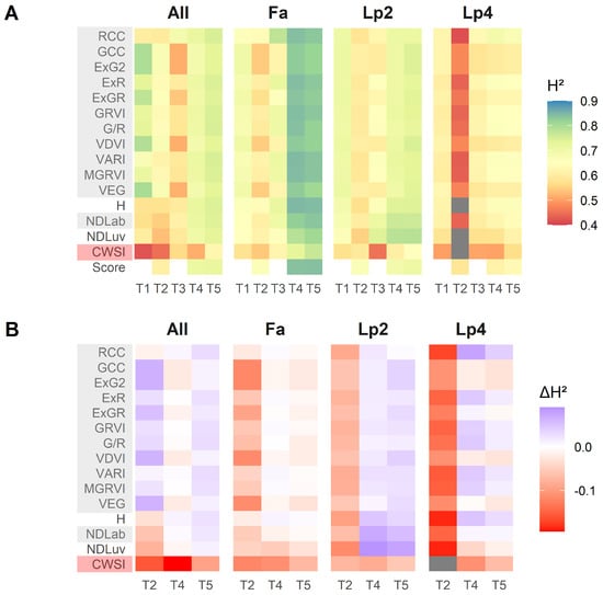
Figure 6.
(A): Broad-sense heritability (H2) calculated per species (Fa: Festuca arundinacea; Lp2: diploid Lolium perenne; Lp4: tetraploid Lolium perenne), per time point (T1–T5) and per index/score. (B): Difference in broad-sense heritability between the breeder score and each of the indices for each species and time point.
The difference in H2 () between the UAV indices and the breeder scores at T2, T4 and T5 (Figure 6B), was in all cases smaller than 0.2. For all species separately, H2 values of the breeder score were higher than the UAV indices at T2, but this was not the case when the data of all species were analysed together (Figure 6B “All”). The behaviour of the data at T4 and T5 was different for each species. For Lp2, all the visual-based indices tended to have higher than the breeder score, whereas for Fa the breeder score tended to perform slightly better than the visual-based indices. For Lp4, several indices outperformed the breeder score (e.g., RCC, ExR, GRVI, G/R, VARI, MGRVI and H), whereas others had lower (GCC, ExG2, VDVI, VEG), or similar values (ExGR, NDLab). When data of the three species were pooled, of the good performing VIs was as good as the breeder score at T4, and slightly better at T5. The thermal index CWSI had lower values than the breeder scores at any time point and any species.
3.4. Contrasting Drought Tolerance Across Species
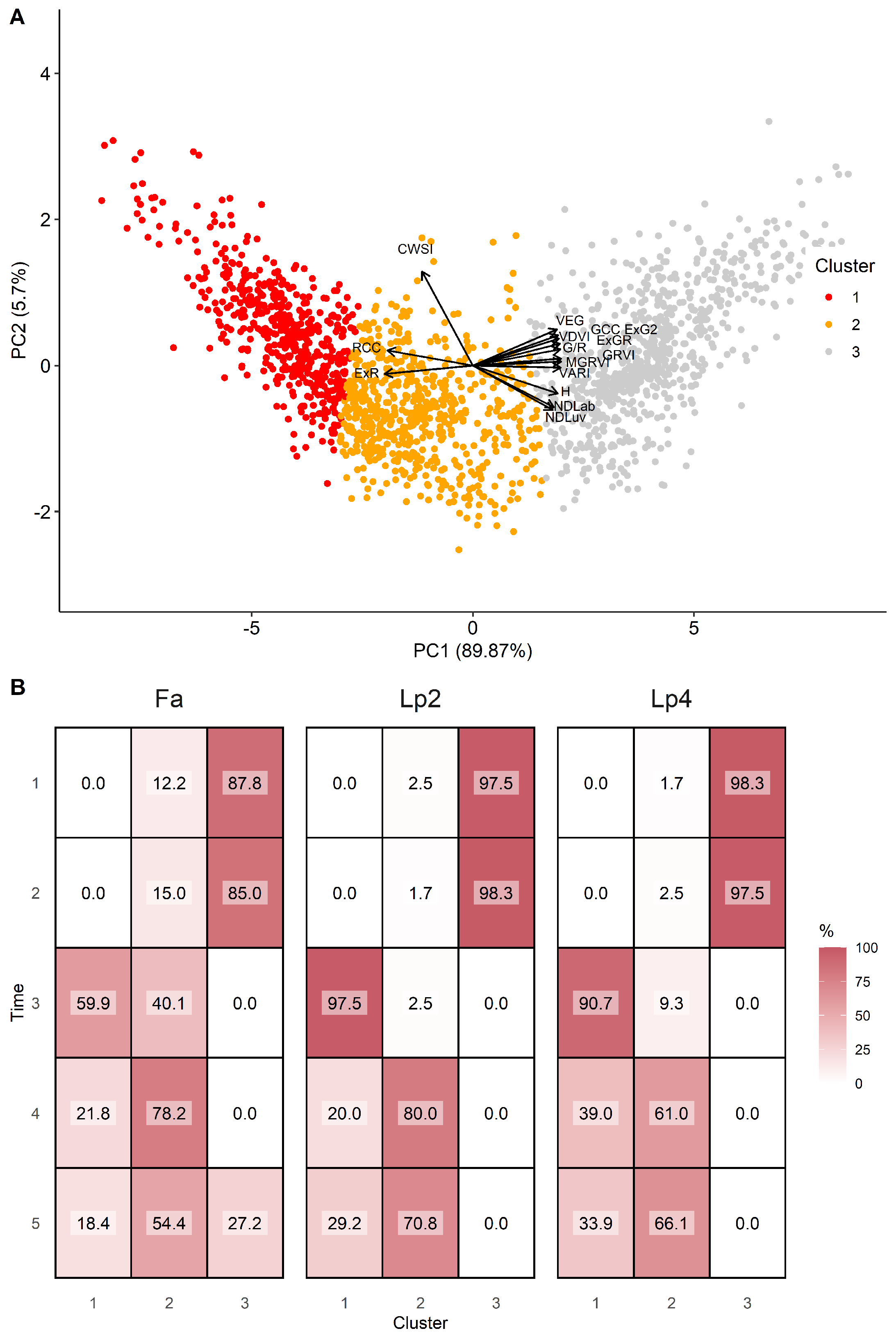
Adjusted means over the three replications were calculated for each selected index, for each time point and each genotype, by taking the block effects of the alpha design into account. The results of the PCA analysis, based on these adjusted means, is shown in Figure 7. This analysis revealed that the visual-based indices are closely correlated and align on the first principal axis (PC1), either positively or negatively. This axis describes 89.9% of the variation present, and can be interpreted as a descriptor of visual appearance, where high values of PC1 indicate greener plants. The second axis (PC2) describes 5.7% of the variation and is particularly related to CWSI. Hence, it can be interpreted as indicating reductions in transpiration. It is noteworthy that all visual indices from the RGB colour space also have a similar score on PC2, whereas the indices from the alternative colour spaces have an opposite score for PC2. These results persist when using only T2, T4 and T5, and including the breeder score in the PCA (Figure S4).
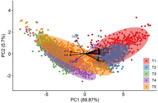
Figure 7.
Two first principal component axes of the Principal Component Analysis (PCA) performed on the individual plant scores per day for the indices RCC, ExR, GCC, ExG2, G/R, GRVI, MGRVI, VARI, VDVI, VEG, H, NDLab, and CWSI. Dots display the projected mean values per genotype and per time point (T1–T5). The Cumulative Water Deficit (CWD) and Volumetric Water Content (VWC) data are presented as a quantitative supplementary variable, but were not used for the PCA.
At T1 and T2, plants had relatively high values on PC1, but a quite large variation on PC2 across genotypes and species, indicating different behaviour in stomatal closure when soil moisture was not yet limiting. At T3, plants scored very low on PC1 (low greenness), as a result of the mowing two days earlier. Data from T4 and T5 present a large variation on both axes and suggest that there is a link between both dimensions as high values on PC1 (greener plants) correspond to low values on PC2 (higher stomatal conductance) and vice versa. To further explore the data by species, we clustered the points according to their score on PC1 and PC2 in three groups (Figure 8). Cluster 1 associated with low values for PC1 and high values of PC2, and thus contained data of plants with reduced transpiration and lower greenness. Cluster 2 contained intermediate data points on both axes, whereas Cluster 3 contained data with high values on PC1, but large variations on the PC2 axis. At T1 and T2, the vast majority of genotypes were classified in Cluster 3, particularly for Lp2 and Lp4. At T3, after mowing, Lp2 and Lp4 genotypes were almost exclusively classified in Cluster 1, with genotypes from Fa distributed evenly across Clusters 1 and 2. At T4 and T5, most plants were classified in Cluster 2 for all species, with the remaining genotypes mostly grouped in Cluster 1. The exception here is Fa at T5, where 27% of the genotypes were classified in Cluster 3. On the other hand, a relatively large portion (37%) of genotypes of Lp4 were in Cluster 1. The PCA results indicate a strong correlation among the indices from the RGB-colour space as well as those between NDLab and NDLuv. For further analysis of species behaviour, we selected the MGRVI index from the RGB colour space, because of its high correlation with the breeder score (Figure 4) and high values for all species at T4 and T5 (Figure 6), along with the H, NDLab, CWSI index and the breeder score.

Figure 8.
Results of the hierarchical cluster analysis, presented via the two major principal components (panel A). The distribution in % of the genotypes per time point (1–5) and per species (Fa: Festuca arundinacea; Lp2: diploid Lolium perenne; Lp4: tetraploid Lolium perenne) in the three clusters (panel B).
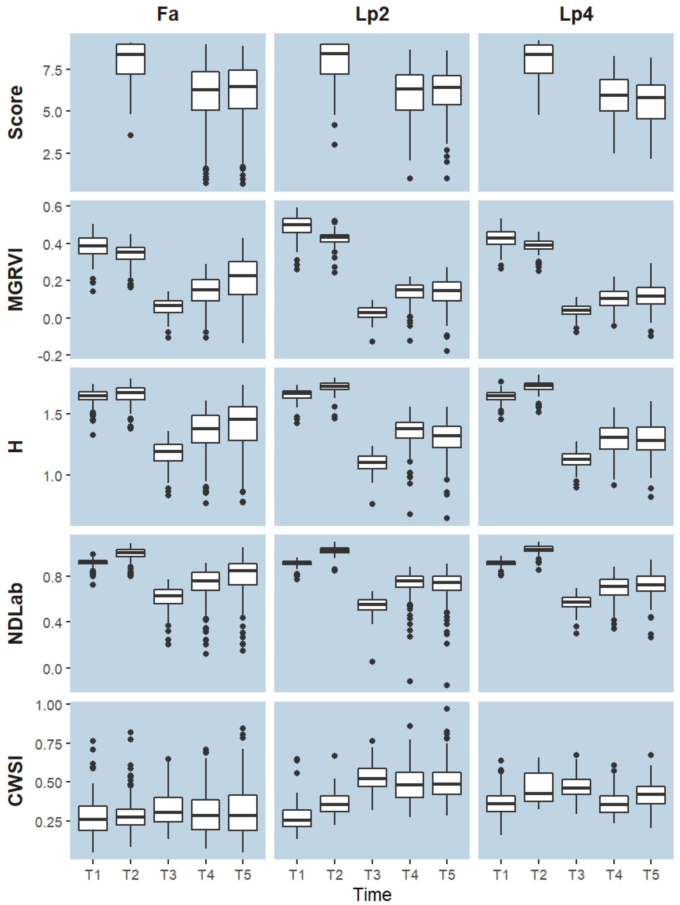
While values of H and NDLab increased from T1 to T2, values of MGRVI index decreased (Figure 9). The reduction in greenness after mowing was clearly visible at T3 for all species and for all visual-based indices. Also for all species, the visual-based indices displayed an overall increase from T3 to T4, which corresponds to growth after mowing, as was also visualised in Figure 9. From T4 to T5, however, the behaviour of the different species is somewhat different and in line with the observations of the PCA. While the median value of all visual-based indices for Fa still increased from T4 to T5, they remained constant or even decreased for Lp2 and Lp4. A similar trend was captured by the breeder score. The median CWSI value for Fa remained more or less constant over time. For Lp2 and Lp4, CWSI increased from T1 to T2 and to T3, and declined again at T4. The median CWSI values of Lp2 at T4 and T5 were higher than those of Lp4. For all species, the median CWSI was highest at T3.
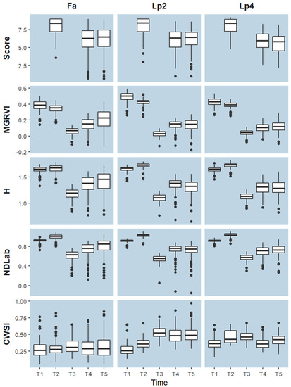
Figure 9.
Boxplots represent the distribution per time point (T1–T5) and species (Fa: Festuca arundinacea; Lp2: diploid Lolium perenne; Lp4: tetraploid Lolium perenne) of the breeder score and four selected indices: MGRVI, H, NDLab and CWSI. Boxes are delimited by the 25th and 75th percentile, horizontal lines indicate the median values. Data are the mean values per genotype and are grouped per time point.
4. Discussion
4.1. Conceptualisation of the Drought Stress Treatment on Grasses
Forage grasses are typically mown multiple times per growing season. As the soil gradually dries out in the absence of rain, the drying period is very likely to include one of the mowing events, as was the case in the present experiment (Figure 2). Due to the mowing, all visual-based indices indicated a clear change at T3 (Figure 9), caused by the removal of green biomass rather than by sudden drought stress. This complicates the comparison of phenotypes before and after the stress treatment, and therefore makes it more challenging to disentangle a genotype’s drought tolerance from other traits that affect regrowth after mowing (e.g., number of growing tips). Regrowth after mowing is substantially impacted by the availability of nutrients, and species and genotypes differ in nutrient use efficiency [79]. Because we wanted to exclude genotypic differences in nutrient use efficiency from biasing the drought response, fertilizer was added after mowing and intermediate rain events were used to ensure that the fertilizer was dissolved and thus available for plant uptake (Figure 2).
4.2. Research Question 1: Visual-Based Indices Are Good Proxies for Breeder Scores
Several VIs correlated very well with the visual breeder scores for the different species (Figure 4). At T2, correlations were lower, but this was related to the lower variation in breeder scores and visual-based indices at that time, when soil moisture was not limiting yet (Figure 3, Figure 5 and Figure 9). Some indices (ExG, G-R, CIVE, a*, ab, u* and uv) displayed high correlations with the breeding score at single time points, but not when data from all time points were pooled. These indices were thus sensitive to the camera settings and to the prevailing environmental conditions at the time of the flight. This sensitivity can possibly be reduced by calibration of the sensor signal and conversion to reflectance values using grey reference panels [80]. However, even without this correction, several other VIs were quite robust to the different sensor settings and conditions, and maintained high correlations with the breeder score when data from all observation days were pooled (Figure 4). The two VIs with the highest overall correlation with the breeder score were H (r = 0.84), from the HSV colour space, and NDLab (r = 0.82), from the CIELab colour space. This confirmed our hypothesis that VIs from alternative colour spaces correlate better with the breeder score than RGB-based VIs, as they are more similar to the colour perception by the human eye [38,39] and less influenced by sensor settings and measurement conditions [40,41]. Nevertheless, it was—to our knowledge—the first time that these two indices were related to visual breeder scores. In phenotyping studies, H and NDLab previously proved useful for predicting grain yield or for assessing disease severity in wheat and maize [39,81,82,83]. MGRVI was the best performing RGB index, although the difference with VARI was minimal. Previous studies on barley and rice suggested that MGRVI is particularly related to biomass and leaf area index, at least in early growth stages [70,84]. This can explain its good performance in our study.
4.3. Research Question 2: Broad-Sense Heritability
A high overall correlation with the breeder score as such is not sufficient in this context. We additionally tested the VIs for their ability to exploit the genotypic variation present in the experiment, by calculating the broad-sense heritability (). VIs that performed well on were able to highlight features that explain differences in drought tolerance, while minimizing potential differences that can be attributed to ‘random factors’. Several VIs actually showed comparable or even better overall values than the breeder score itself (Figure 6B), although there was a strong difference across the species and time points. Apparently, the VIs performed worse than the breeder score at T2, when drought was not yet impacting the plants, and the spread on the data was small (Figure 3 and Figure 9). Potentially, this could be attributed to a certain level of saturation of the VIs, as the Leaf Area Index became high. However, this disadvantage at T2 disappeared when taking all species together (Figure 6B). At T4 and T5, several indices performed comparably (especially for Fa), or better (for Lp2 and Lp4) than the breeder score. As a final selection, the VIs with very high correlation to the breeder score, but with comparable or better values for all species included H, NDLab and MGRVI, and, to a lesser extent, RCC, ExR, GRVI, G/R and VARI Figure 4, Figure 6 and Figure 7. These are thus the best candidates for replacing or complementing the breeder scores in future studies.
Some of these indices were also highly correlated to each other and were intrinsically reflecting very similar properties. Still, more detailed analyses also revealed differences between on the one hand the RGB-based indices, such as MGRVI, and on the other hand H and NDLab (Figure 9): from T1 to T2, MGRVI (as well as other RGB-based indices, data not shown) decreased whereas H and NDLab increased. As the volumetric water content at T2 was still quite high (83% REW), we expect that plants were still growing between T1 and T2. This would imply that H and NDLab are better proxies for plant vigour. On the other hand, the CWSI index also showed a slight increase, thus indicating a slightly more stressed condition. These higher CWSI values, especially for Lp2 and Lp4, could however also be attributed to the higher evaporative demand at T2, compared to T1 (Table 1). The reason for the differences in the trend from T1 to T2 was not entirely clear. The main difference in plant state between T1 and T2 was the size of the plants—which was larger at T2, with grass leaves bending over. This change in leaf orientation could be a possible explanation for the diverging signal – with leaves bending over, more leaves are reflecting very strongly in all bands, causing a drop in MGRVI (Table 2). Moreover, the images on T2 were also slightly darker (mean overall was 73, versus 206 on T1—See also Figure S2). Colour space transformations as HSV and CIELab are developed to be less sensitive for these illumination issues, caused by camera settings or leaf orientation [41].
4.4. Research Question 3: Added Value of Thermal Indices
Although and CWSI were significantly correlated with the breeder score (Figure 4, Table S1), it was clear that the visual-based VIs were more useful as complement or replacement of the breeder score. Nevertheless, CWSI reflects the actual transpiration [51,85], and as the PCA analysis confirmed (Figure 7), CWSI can be used as an additional and complementary source of information for selection. The data confirmed that when drought stress was not present or was very moderate, the range in CWSI was large, despite a relatively uniform greenness of the canopy. When drought stress became more severe, CWSI and RGB-based VIs were more closely correlated (Figure S5). CWSI values at T1 and T2 were not highly correlated to CWSI at T5 (r = 0.11 and r = 0.28, respectively), suggesting that the genotypes that transpired more vigorously under normal growing conditions did not necessarily maintain high transpiration under drought conditions.
4.5. Research Question 4: Distinct Behaviour within and between the Species
A slight increase in CWSI was observed from T1 to T2 for both Lp species, but not for Fa (Figure 9). At T2, soil water availability was not yet limiting (83% REW, Figure 2), but VPD was high (3.06 kPa, versus 2.51 kPa at T1) (Table 1), suggesting that Lp has a more strict stomatal regulation to atmospheric conditions than Fa. This confirmed other studies that reported larger stomatal conductance values of Fa under control conditions [15] and stomatal closure occurring at lower (i.e., more negative) leaf water potential than Lp [86,87]. These differences in stomatal control can be caused by several mechanisms. First, differences in leaf hydraulic conductance can cause variations in water transport limitations [88,89]. Second, hydraulics at the soil-root interface can play a role [90]. In comparison with Lp, Fa has substantially more root biomass in deeper soil layers than Lp grasses [14,91]. Hence, it is plausible that plants with a relatively small rooting system can experience an insufficient hydraulic conductance under conditions of high evaporative demand [90,92]. At T3, all visual-based indices showed a strong reduction in greenness (Figure 3 and Figure 7, Figure 8 and Figure 9), as a result of mowing, but overall levels of Fa remained higher. The CWSI of Fa remained lower than that of Lp2 and Lp4 (Figure 9), probably as a combination of the larger green leaf area and the more limited stomatal control (VPD = 4.0 kPa, Table 1). At T4, the median value of all visual-based indices increased for all species compared to T3 (Figure 9), confirming the regrowth after mowing. In line with this, the CWSI of Lp2 and Lp4 decreased compared to T3, although this can also be due to less demanding meteorological conditions (VPD of 2.7 kPa at T4 versus 4.0 kPa at T3). However, the CWSI levels for both Lp species remained higher than for Fa (Figure 9). From T4 to T5, with increasing limitation in available water, the species responded differently in terms of visual-based indices H, NDLab and MGRVI (Figure 9). Where the median values of Fa continued to increase, this increment was no longer visible in Lp2 and Lp4 (Figure 9), as was also confirmed by the cluster analysis (Figure 8). The lower CWSI of Fa at T5 further confirmed the higher drought tolerance of Fa. CWSI values of Lp4 were generally higher than those of Lp2 at T1 and T2 (Figure 9). This confirmed former findings, where modified stomatal density and pore size tend to reduce the transpiration per unit of leaf area of tetraploids compared to diploids for different species [93,94]. In the recovery from T3 to T4, the increase of visual-based indices, and hence the regrowth, was also higher for Lp2 than for Lp4. Yet, at T4 and T5, Lp4 tended to have a lower CWSI than Lp2. Potentially, the lower transpiration rates in tetraploid genotypes in non-stressed conditions conserved more water, resulting in a delay of drought stress effects.
4.6. Future Perspectives
In this research, we illustrated that consumer-grade RGB cameras can be used to complement or replace the visual breeder score in forage grasses. This allows breeder score assessments with affordable UAVs by pilots who are not necessarily remote sensing experts. In order to be routinely applied in high throughput phenotyping studies, the data processing should also be straightforward. Nowadays, the computation of orthophotos from RGB imagery using structure-from-motion software is largely automated. In this respect, it is recommended to place permanent ground control points (GCPs) with known coordinates in the experimental field, in a way that they remain visible throughout the entire experiment. The calculation of vegetation indices such as H, NDLab or MGRVI from the orthophotos, and the final estimation of the breeder score, can also be completely automated. Although reference grey panels were not used in this research, they can probably further increase the robustness of vegetation indices.
A further development considers the fate of the visual breeder score itself. With more advanced UAV remote sensing technology, the breeder score’s qualitative assessment of greenness and biomass can be translated to more objective and quantitative variables. Plant biomass can be estimated from vegetation indices in the visual and near infrared wavelengths, from the 3D vegetation model, obtained through structure-from-motion software from UAV-based RGB or multispectral data, or from their combination [34].
The plant greenness aspect of the breeder score can relate to two aspects. First, it can relate to the chlorophyll content in the leaves. In breeding studies, this is particularly useful when investigating the stress-sensitivity of the different genotypes [95]. Chlorophyll content can be best quantified with vegetation indices based on spectra in the red edge [34]. Other indices, such as NDVI, are sensitive to both leaf area index and chlorophyll content, and have already demonstrated high correlations with breeder scores [25]. On the other hand, plant greenness can also relate to the digestibility of forage grasses. Digestibility can be measured routinely with NIRS (near-infrared spectroscopy) analyses, from which parameters as the D-value (digestibility of organic matter in dry matter), WSC (water soluble carbohydrates) or similar feed quality features can be predicted [96]. However, NIRS uses destructive sampling and is too costly and time-intensive for large scale application in breeding programs [97]. Several studies indicate that hand-held hyperspectral sensors can provide a non-destructive and fast alternative, possibly suited for breeding purposes [97,98,99]. Hyperspectral sensing from UAVs has been demonstrated to be suitable for estimating forage grass digestibility [96]. However, more research is needed to overcome several remaining challenges, which are particularly related to the poor general applicability of the established empirical regressions across the seasons and years [100,101].
5. Conclusions
Using rainout shelters, a field experiment was set up to evaluate drought stress tolerance on a large number of genotypes of the forage grass species Festuca arundinacea (Fa), diploid Lolium perenne (Lp2) and Lolium perenne (Lp4) in a breeding context using RGB and thermal UAV imagery. We identified several visual-based indices that showed high correlations with the breeder scores and displayed high ‘broad-sense’ heritability. These indices can serve as a proxy for breeder scores, for which dedicated pipelines can be set up to automate the processing and potentially increase consistency of selection. In particular, the use of H, NDLab and MGRVI can be considered for this purpose. The thermal index CWSI provided complementary information to visual indices, and this enabled the analysis of differences in ecophysiological mechanisms for coping with reduced water availability. The panel of Fa genotypes displayed the largest variation across all indices. Overall, CWSI was lowest for Fa, which also showed the best regrowth after mowing under water-limiting conditions, confirming the good drought tolerance of Fa. Nevertheless, substantial variation was found also among the diploid and tetraploid L. perenne genotypes, which can be exploited for breeding towards better drought stress tolerance in this species.
Supplementary Materials
The following are available online at https://www.mdpi.com/2072-4292/13/1/147/s1. Figure S1: Spectral response of the RGB camera (Canon S110) used in this study. Figure S2: Detailed view of the Lp2-block (indicated by the thick, dark-red line) of the middle row (see also Figure 1, main text) for the five different time points and for the RGB orthophoto (above) and surface temperature orthophoto (below). The red polygons illustrate the plant polygons in this block used for the data analyses. Figure S3: Volumetric Water Content (VWC) for different soil depths (from 10 to 80 cm). Blue lines are the mean of three sensors (one in each rainout shelter). The grey shaded area represents the 95% confidence interval on the VWC data of the 18 sensors monitoring the 10–40 cm soil profile. Figure S4: Two first principal component axes of the Principal Component Analysis (PCA) performed on the individual genotype values per day for the breeder scores and the indices RCC, ExR, GCC, ExG2, G/R, GRVI, MGRVI, VARI, VDVI, VEG, H, NDLab, and CWSI. Dots display the projected mean values per genotype and per time point (T2, T4 and T5). The Cumulative Water Deficit (CWD) and Volumetric Water Content (VWC) data are presented as a quantitative supplementary variable, but were not used for the PCA. Figure S5: Absolute values of Pearson correlations (|r|) between selected vegetation indices for five time points (T1–T5) and for all species (Fa: Festuca arundinacea, Lp2: diploid Lolium perenne, Lp4: tetraploid Lolium perenne. Table S1: Pearson correlations between all 37 indices and the breeder score for the individual species (Fa: Festuca arundinacea; Lp2: diploid Lolium perenne; Lp4: tetraploid Lolium perenne), and all species pooled together (All), and for the individual time points (T2, T4, T5) and all time points pooled together (All).
Author Contributions
Conceptualization, T.D.S. and W.H.M.; methodology, T.D.S., W.H.M., J.A.; formal analysis, T.D.S., W.H.M. and P.L.; investigation, T.D.S., W.H.M., J.A. and P.L.; resources, M.C., D.R., J.A., J.B., W.H.M.; data curation, J.A., P.L., T.D.S. and W.H.M.; writing–original draft preparation, P.L., T.D.S. and W.H.M.; writing–review and editing, P.L., I.R.-R., D.R., M.C., K.S.; visualization, T.D.S. and W.H.M. All authors have read and agreed to the published version of the manuscript.
Funding
At the time of measurement, W.H.M. was funded by the Special Research Fund (BOF) from Ghent University.
Institutional Review Board Statement
Not applicable.
Informed Consent Statement
Not applicable.
Data Availability Statement
Data is publicly available at https://zenodo.org/record/4415643#.X_Z2ZBYRWUk.
Acknowledgments
The authors thank the ILVO field trial team for installing and maintaining the field trial, as well as three anonymous reviewers for their constructive feedback.
Conflicts of Interest
The authors declare no conflict of interest.
Abbreviations
The following abbreviations are used in this manuscript:
| CWD | Cumulative Water Deficit |
| ET0 | Reference evapotranspiration |
| Fa | diploid Festuca arundinacea Schreb. |
| GCP | Ground Control Point |
| H2 | broad-sense heritability |
| HSL | Hue, Saturation, Luminosity |
| HSV | Hue, Saturation, Value |
| Lp2 | diploid Lolium perenne L. |
| Lp4 | tetraploid Lolium perenne L. |
| NDVI | Normalized Difference Vegetation Index |
| NIRS | Near Infra-Red Spectroscopy |
| P | Precipitation |
| PCA | Principal Component analysis |
| r | correlation |
| REW | Relative Extractable Water |
| RGB | Red, Green, Blue |
| T1–T5 | Time point 1 to 5 |
| Tair | Air temperature |
| Tbr | Brightness temperature |
| Tdry | Leaf surface temperature of non-transpiring plant |
| Tpot | Leaf surface temperature of maximal transpiring plant |
| Ts | Leaf surface temperature |
| UAV | Unmanned Aerial Vehicle |
| Genotypic variance | |
| Phenotypic variance | |
| VPD | Vapour Pressure Deficit |
| VWC | Volumetric Water Content |
| WSC | Water Soluble Carbohydrates |
References
- FAOSTAT. Available online: http://www.fao.org/faostat/en/#data/RL (accessed on 27 October 2020).
- Huyghe, C.; De Vliegher, A.; van Gils, B.; Peeters, A. Grasslands and Herbivore Production in Europe and Effects of Common Policies; Editions Quae: Versailles, France, 2014. [Google Scholar]
- Soussana, J.F.; Lemaire, G. Coupling carbon and nitrogen cycles for environmentally sustainable intensification of grasslands and crop-livestock systems. Agric. Ecosyst. Environ. 2014, 190, 9–17. [Google Scholar] [CrossRef]
- Kipling, R.P.; Virkajärvi, P.; Breitsameter, L.; Curnel, Y.; De Swaef, T.; Gustavsson, A.M.; Hennart, S.; Höglind, M.; Järvenranta, K.; Minet, J.; et al. Key challenges and priorities for modelling European grasslands under climate change. Sci. Total. Environ. 2016, 566–567, 851–864. [Google Scholar] [CrossRef] [PubMed]
- Blum, A. Plant Breeding for Water-Limited Environments; Life Sciences; Springer: New York, NY, USA, 2010. [Google Scholar]
- Olesen, J.; Trnka, M.; Kersebaum, K.; Skjelvåg, A.; Seguin, B.; Peltonen-Sainio, P.; Rossi, F.; Kozyra, J.; Micale, F. Impacts and adaptation of European crop production systems to climate change. Eur. J. Agron. 2011, 34, 96–112. [Google Scholar] [CrossRef]
- IPCC. Climate Change 2013: The Physical Science Basis. Contribution of Working Group I to the Fifth Assessment Report of the Intergovernmental Panel on Climate Change; Cambridge University Press: Cambridge, UK; New York, NY, USA, 2013. [Google Scholar] [CrossRef]
- Chang, J.; Ciais, P.; Viovy, N.; Soussana, J.F.; Klumpp, K.; Sultan, B. Future productivity and phenology changes in European grasslands for different warming levels: Implications for grassland management and carbon balance. Carbon Balance Manag. 2017, 12, 11. [Google Scholar] [CrossRef] [PubMed]
- Dellar, M.; Topp, C.F.E.; Banos, G.; Wall, E. A meta-analysis on the effects of climate change on the yield and quality of European pastures. Agric. Ecosyst. Environ. 2018, 265, 413–420. [Google Scholar] [CrossRef]
- Cyriac, D.; Hofmann, R.W.; Stewart, A.; Sathish, P.; Winefield, C.S.; Moot, D.J. Intraspecific differences in long-term drought tolerance in perennial ryegrass. PLoS ONE 2018, 13, e0194977. [Google Scholar] [CrossRef] [PubMed]
- Hague, L.M.; Jones, R.N. Cytogenetics of Lolium perenne. Theor. Appl. Genet. 1987, 74, 233–241. [Google Scholar] [CrossRef] [PubMed]
- Humphreys, M.; Feuerstein, U.; Vandewalle, M.; Baert, J. Ryegrasses. In Fodder Crops and Amenity Grasses; Handbook of Plant Breeding; Boller, B., Posselt, U.K., Veronesi, F., Eds.; Springer: New York, NY, USA, 2010; pp. 211–260. [Google Scholar] [CrossRef]
- Turner, L.R.; Holloway-Phillips, M.M.; Rawnsley, R.P.; Donaghy, D.J.; Pembleton, K.G. The morphological and physiological responses of perennial ryegrass (Lolium perenne L.), cocksfoot (Dactylis glomerata L.) and tall fescue (Festuca arundinacea Schreb.; syn. Schedonorus phoenix Scop.) to variable water availability. Grass Forage Sci. 2012, 67, 507–518. [Google Scholar] [CrossRef]
- Cougnon, M.; De Swaef, T.; Lootens, P.; Baert, J.; De Frenne, P.; Shahidi, R.; Roldán-Ruiz, I.; Reheul, D. In situ quantification of forage grass root biomass, distribution and diameter classes under two N fertilisation rates. Plant Soil 2017, 411, 409–422. [Google Scholar] [CrossRef]
- Fariaszewska, A.; Aper, J.; Van Huylenbroeck, J.; De Swaef, T.; Baert, J.; Pecio, L. Physiological and biochemical besponses of forage grass varieties to mild drought stress under field conditions. Int. J. Plant Prod. 2020, 14, 335–353. [Google Scholar] [CrossRef]
- Parra, A.; Ramírez, D.A.; Resco, V.; Velasco, A.; Moreno, J.M. Modifying rainfall patterns in a Mediterranean shrubland: System design, plant responses, and experimental burning. Int. J. Biometeorol. 2012, 56, 1033–1043. [Google Scholar] [CrossRef] [PubMed]
- Poorter, H.; Bühler, J.; Dusschoten, D.V.; Climent, J.; Postma, J.A. Pot size matters: A meta-analysis of the effects of rooting volume on plant growth. Funct. Plant Biol. 2012, 39, 839–850. [Google Scholar] [CrossRef] [PubMed]
- Downes, S.M.; Matthews, L. Heritability. In The Stanford Encyclopedia of Philosophy, 2020th ed.; Zalta, E.N., Ed.; Metaphysics Research Lab, Stanford University: Stanford, CA, USA, 2020. [Google Scholar]
- Borra-Serrano, I.; De Swaef, T.; Aper, J.; Ghesquiere, A.; Mertens, K.; Nuyttens, D.; Saeys, W.; Somers, B.; Vangeyte, J.; Roldán-Ruiz, I.; et al. Towards an objective evaluation of persistency of Lolium perenne swards using UAV imagery. Euphytica 2018, 214, 142. [Google Scholar] [CrossRef]
- Milberg, P.; Bergstedt, J.; Fridman, J.; Odell, G.; Westerberg, L. Observer bias and random variation in vegetation monitoring data. J. Veg. Sci. 2008, 19, 633–644. [Google Scholar] [CrossRef]
- Araus, J.L.; Cairns, J.E. Field high-throughput phenotyping: The new crop breeding frontier. Trends Plant Sci. 2014, 19, 52–61. [Google Scholar] [CrossRef] [PubMed]
- Shakoor, N.; Lee, S.; Mockler, T.C. High throughput phenotyping to accelerate crop breeding and monitoring of diseases in the field. Curr. Opin. Plant Biol. 2017, 38, 184–192. [Google Scholar] [CrossRef] [PubMed]
- Tucker, C.J. Red and photographic infrared linear combinations for monitoring vegetation. Remote Sens. Environ. 1979, 8, 127–150. [Google Scholar] [CrossRef]
- Huete, A.R. A soil-adjusted vegetation index (SAVI). Remote Sens. Environ. 1988, 25, 295–309. [Google Scholar] [CrossRef]
- Wang, J.; Badenhorst, P.; Phelan, A.; Pembleton, L.; Shi, F.; Cogan, N.; Spangenberg, G.; Smith, K. Using sensors and unmanned aircraft systems for high-throughput phenotyping of biomass in perennial ryegrass breeding trials. Front. Plant Sci. 2019, 10, 1381. [Google Scholar] [CrossRef]
- Araus, J.L.; Kefauver, S.C. Breeding to adapt agriculture to climate change: Affordable phenotyping solutions. Curr. Opin. Plant Biol. 2018, 45, 237–247. [Google Scholar] [CrossRef]
- Rebetzke, G.J.; Jimenez-Berni, J.; Fischer, R.A.; Deery, D.M.; Smith, D.J. Review: High-throughput phenotyping to enhance the use of crop genetic resources. Plant Sci. 2019, 282, 40–48. [Google Scholar] [CrossRef] [PubMed]
- Pieruschka, R.; Schurr, U. Plant phenotyping: Past, present, and future. Plant Phenomics 2019, 2019, 7507131. [Google Scholar] [CrossRef] [PubMed]
- Perich, G.; Hund, A.; Anderegg, J.; Roth, L.; Boer, M.P.; Walter, A.; Liebisch, F.; Aasen, H. Assessment of multi-image unmanned aerial vehicle based high-throughput field phenotyping of canopy temperature. Front. Plant Sci. 2020, 11, 150. [Google Scholar] [CrossRef] [PubMed]
- Travlos, I.; Mikroulis, A.; Anastasiou, E.; Fountas, S.; Bilalis, D.; Tsiropoulos, Z.; Balafoutis, A. The use of RGB cameras in defining crop development in legumes. Adv. Anim. Biosci. 2017, 8, 224–228. [Google Scholar] [CrossRef]
- Vergara-Díaz, O.; Zaman-Allah, M.A.; Masuka, B.; Hornero, A.; Zarco-Tejada, P.; Prasanna, B.M.; Cairns, J.E.; Araus, J.L. A novel remote sensing approach for prediction of maize yield under different conditions of nitrogen fertilization. Front. Plant Sci. 2016, 7, 666. [Google Scholar] [CrossRef] [PubMed]
- Gracia-Romero, A.; Kefauver, S.C.; Vergara-Díaz, O.; Zaman-Allah, M.A.; Prasanna, B.M.; Cairns, J.E.; Araus, J.L. Comparative performance of ground vs. aerially assessed RGB and multispectral indices for early-growth evaluation of maize performance under phosphorus fertilization. Front. Plant Sci. 2017, 8, 2004. [Google Scholar] [CrossRef]
- Jiménez-Brenes, F.M.; López-Granados, F.; Torres-Sánchez, J.; Peña, J.M.; Ramírez, P.; Castillejo-González, I.L.; Castro, A.I.D. Automatic UAV-based detection of Cynodon dactylon for site-specific vineyard management. PLoS ONE 2019, 14, e0218132. [Google Scholar] [CrossRef]
- Maes, W.H.; Steppe, K. Perspectives for remote sensing with unmanned aerial vehicles in precision agriculture. Trends Plant Sci. 2019, 24, 152–164. [Google Scholar] [CrossRef]
- Woebbecke, M.D.; Meyer, E.G.; Von Bargen, K.; Mortensen, A.D. Color indices for weed identification under various soil, residue, and lighting conditions. Trans. ASAE 1995, 38, 259–269. [Google Scholar] [CrossRef]
- Hunt, E.R.; Cavigelli, M.; Daughtry, C.S.T.; Mcmurtrey, J.E.; Walthall, C.L. Evaluation of digital photography from model aircraft for remote sensing of crop biomass and nitrogen status. Precis. Agric. 2005, 6, 359–378. [Google Scholar] [CrossRef]
- Gitelson, A.A.; Kaufman, Y.J.; Stark, R.; Rundquist, D. Novel algorithms for remote estimation of vegetation fraction. Remote Sens. Environ. 2002, 80, 76–87. [Google Scholar] [CrossRef]
- Hernández-Hernández, J.L.; García-Mateos, G.; González-Esquiva, J.M.; Escarabajal-Henarejos, D.; Ruiz-Canales, A.; Molina-Martínez, J.M. Optimal color space selection method for plant/soil segmentation in agriculture. Comput. Electron. Agric. 2016, 122, 124–132. [Google Scholar] [CrossRef]
- Buchaillot, M.L.; Gracia-Romero, A.; Vergara-Diaz, O.; Zaman-Allah, M.A.; Tarekegne, A.; Cairns, J.E.; Prasanna, B.M.; Araus, J.L.; Kefauver, S.C. Evaluating maize genotype performance under low nitrogen conditions using RGB UAV phenotyping techniques. Sensors 2019, 19, 1815. [Google Scholar] [CrossRef] [PubMed]
- Philipp, I.; Rath, T. Improving plant discrimination in image processing by use of different colour space transformations. Comput. Electron. Agric. 2002, 35, 1–15. [Google Scholar] [CrossRef]
- Sadeghi-Tehran, P.; Virlet, N.; Sabermanesh, K.; Hawkesford, M.J. Multi-feature machine learning model for automatic segmentation of green fractional vegetation cover for high-throughput field phenotyping. Plant Methods 2017, 13, 103. [Google Scholar] [CrossRef] [PubMed]
- Song, W.; Mu, X.; Yan, G.; Huang, S. Extracting the green fractional vegetation cover from digital images using a shadow-resistant algorithm (SHAR-LABFVC). Remote Sens. 2015, 7, 10425–10443. [Google Scholar] [CrossRef]
- Lootens, P.; Ruttink, T.; Rohde, A.; Combes, D.; Barre, P.; Roldán-Ruiz, I. High-throughput phenotyping of lateral expansion and regrowth of spaced Lolium perenne plants using on-field image analysis. Plant Methods 2016, 12, 32. [Google Scholar] [CrossRef]
- Li, L.; Mu, X.; Macfarlane, C.; Song, W.; Chen, J.; Yan, K.; Yan, G. A half-Gaussian fitting method for estimating fractional vegetation cover of corn crops using unmanned aerial vehicle images. Agric. For. Meteorol. 2018, 262, 379–390. [Google Scholar] [CrossRef]
- Suh, H.K.; Hofstee, J.W.; van Henten, E.J. Improved vegetation segmentation with ground shadow removal using an HDR camera. Precis. Agric. 2018, 19, 218–237. [Google Scholar] [CrossRef]
- Rico-Fernández, M.P.; Rios-Cabrera, R.; Castelán, M.; Guerrero-Reyes, H.I.; Juarez-Maldonado, A. A contextualized approach for segmentation of foliage in different crop species. Comput. Electron. Agric. 2019, 156, 378–386. [Google Scholar] [CrossRef]
- Kim, J.; Kang, S.; Seo, B.; Narantsetseg, A.; Han, Y. Estimating fractional green vegetation cover of Mongolian grasslands using digital camera images and MODIS satellite vegetation indices. Gisci. Remote Sens. 2020, 57, 49–59. [Google Scholar] [CrossRef]
- Kerkech, M.; Hafiane, A.; Canals, R. Deep learning approach with colorimetric spaces and vegetation indices for vine diseases detection in UAV images. Comput. Electron. Agric. 2018, 155, 237–243. [Google Scholar] [CrossRef]
- Serret, M.D.; Al-Dakheel, A.J.; Yousfi, S.; Fernández-Gallego, J.A.; Elouafi, I.A.; Araus, J.L. Vegetation indices derived from digital images and stable carbon and nitrogen isotope signatures as indicators of date palm performance under salinity. Agric. Water Manag. 2020, 230, 105949. [Google Scholar] [CrossRef]
- Borra-Serrano, I.; De Swaef, T.; Muylle, H.; Nuyttens, D.; Vangeyte, J.; Mertens, K.; Saeys, W.; Somers, B.; Roldán-Ruiz, I.; Lootens, P. Canopy height measurements and non-destructive biomass estimation of Lolium perenne swards using UAV imagery. Grass Forage Sci. 2019, 74, 356–369. [Google Scholar] [CrossRef]
- Maes, W.H.; Steppe, K. Estimating evapotranspiration and drought stress with ground-based thermal remote sensing in agriculture: A review. J. Exp. Bot. 2012, 63, 4671–4712. [Google Scholar] [CrossRef] [PubMed]
- Gerhards, M.; Schlerf, M.; Rascher, U.; Udelhoven, T.; Juszczak, R.; Alberti, G.; Miglietta, F.; Inoue, Y. Analysis of airborne optical and thermal imagery for detection of water stress symptoms. Remote Sens. 2018, 10, 1139. [Google Scholar] [CrossRef]
- Ludovisi, R.; Tauro, F.; Salvati, R.; Khoury, S.; Mugnozza Scarascia, G.; Harfouche, A. UAV-based thermal imaging for high-throughput field phenotyping of black poplar response to drought. Front. Plant Sci. 2017, 8, 1681. [Google Scholar] [CrossRef]
- Dillen, M.; Vanhellemont, M.; Verdonckt, P.; Maes, W.H.; Steppe, K.; Verheyen, K. Productivity, stand dynamics and the selection effect in a mixed willow clone short rotation coppice plantation. Biomass Bioenergy 2016, 87, 46–54. [Google Scholar] [CrossRef]
- Gracia-Romero, A.; Kefauver, S.C.; Fernandez-Gallego, J.A.; Vergara-Díaz, O.; Nieto-Taladriz, M.T.; Araus, J.L. UAV and ground image-based phenotyping: A proof of concept with durum wheat. Remote Sens. 2019, 11, 1244. [Google Scholar] [CrossRef]
- Kaler, A.S.; Ray, J.D.; Schapaugh, W.T.; Asebedo, A.R.; King, C.A.; Gbur, E.E.; Purcell, L.C. Association mapping identifies loci for canopy temperature under drought in diverse soybean genotypes. Euphytica 2018, 214, 135. [Google Scholar] [CrossRef]
- Natarajan, S.; Basnayake, J.; Wei, X.; Lakshmanan, P. High-throughput phenotyping of indirect traits for early-stage selection in sugarcane breeding. Remote Sens. 2019, 11, 2952. [Google Scholar] [CrossRef]
- De Mendiburu, F. Agricolae: Statistical Procedures for Agricultural Research. 2020. Available online: https://CRAN.R-project.org/package=agricolae (accessed on 29 December 2020).
- R Core Team. R: A Language and Environment for Statistical Computing; R Foundation for Statistical Computing: Vienna, Austria, 2020. [Google Scholar]
- Allen, R.G.; Pereira, L.S.; Raes, D.; Smith, M. Crop Evapotranspiration—Guidelines for Computing Crop Water Requirements—FAO Irrigation and Drainage Paper 56; FAO: Rome, Italy, 1998; p. 15. [Google Scholar]
- Guo, D.; Westra, S.; Peterson, T. Evapotranspiration: Modelling Actual, Potential and Reference Crop Evapotranspiration. 2020. Available online: https://CRAN.R-project.org/package=Evapotranspiration (accessed on 29 December 2020).
- Maes, W.H.; Huete, A.R.; Steppe, K. Optimizing the processing of UAV-based thermal imagery. Remote Sens. 2017, 9, 476. [Google Scholar] [CrossRef]
- Maes, W.H.; Huete, A.R.; Avino, M.; Boer, M.M.; Dehaan, R.; Pendall, E.; Griebel, A.; Steppe, K. Can UAV-based infrared thermography be used to study plant-parasite interactions between mistletoe and eucalypt trees? Remote Sens. 2018, 10, 2062. [Google Scholar] [CrossRef]
- Berra, E.F.; Gaulton, R.; Barr, S. Commercial off-the-shelf digital cameras on unmanned aerial vehicles for multitemporal monitoring of vegetation reflectance and NDVI. IEEE Trans. Geosci. Remote. Sens. 2017, 55, 4878–4886. [Google Scholar] [CrossRef]
- De Kock, M.; Gallacher, D. From Drone Data to Decisions: Turning Images into Ecological Answers. In Proceedings of the Innovation Arabia 9, Dubai, UAE, 7–9 March 2016. [Google Scholar] [CrossRef]
- Meyer, G.E.; Hindman, T.W.; Laksmi, K. Machine vision detection parameters for plant species identification. In Proceedings of the Precision Agriculture and Biological Quality, Boston, MA, USA, 3–4 November 1999; Volume 3543, pp. 327–335. [Google Scholar] [CrossRef]
- Meyer, G.E.; Camargo Neto, J.; Jones, D.D.; Hindman, T.W. Intensified fuzzy clusters for classifying plant, soil, and residue regions of interest from color images. Comput. Electron. Agric. 2004, 42, 161–180. [Google Scholar] [CrossRef]
- Steele, M.R.; Gitelson, A.A.; Rundquist, D.C.; Merzlyak, M.N. Nondestructive estimation of anthocyanin content in grapevine leaves. Am. J. Enol. Vitic. 2009, 60, 87–92. [Google Scholar]
- Xiaoqin, W.; Miaomiao, W.; Shaoqiang, W.; Yundong, W. Extraction of vegetation information from visible unmanned aerial vehicle images. Trans. Chin. Soc. Agric. Eng. 2015, 31, 152–159. [Google Scholar]
- Bendig, J.; Yu, K.; Aasen, H.; Bolten, A.; Bennertz, S.; Broscheit, J.; Gnyp, M.L.; Bareth, G. Combining UAV-based plant height from crop surface models, visible, and near infrared vegetation indices for biomass monitoring in barley. Int. J. Appl. Earth Obs. Geoinf. 2015, 39, 79–87. [Google Scholar] [CrossRef]
- Kataoka, T.; Kaneko, T.; Okamoto, H.; Hata, S. Crop growth estimation system using machine vision. In Proceedings of the 2003 IEEE/ASME International Conference on Advanced Intelligent Mechatronics (AIM 2003), Kobe, Japan, 20–24 July 2003; Volume 2, pp. b1079–b1083. [Google Scholar] [CrossRef]
- Hague, T.; Tillett, N.D.; Wheeler, H. Automated crop and weed monitoring in widely spaced cereals. Precis. Agric. 2006, 7, 21–32. [Google Scholar] [CrossRef]
- Cheng, H.D.; Jiang, X.H.; Sun, Y.; Wang, J. Color image segmentation: Advances and prospects. Pattern Recognit. 2001, 34, 2259–2281. [Google Scholar] [CrossRef]
- Idso, S.B.; Reginato, R.J.; Jackson, R.D.; Pinter, P.J. Measuring yield-reducing plant water potential depressions in wheat by infrared thermometry. Irrig. Sci. 1981, 2, 205–212. [Google Scholar] [CrossRef]
- Park, S.; Ryu, D.; Fuentes, S.; Chung, H.; Hernández-Montes, E.; O’Connell, M. Adaptive estimation of crop water stress in nectarine and peach orchards using high-resolution imagery from an unmanned aerial vehicle (UAV). Remote Sens. 2017, 9, 828. [Google Scholar] [CrossRef]
- Bian, J.; Zhang, Z.; Chen, J.; Chen, H.; Cui, C.; Li, X.; Chen, S.; Fu, Q. Simplified evaluation of cotton water stress using high resolution unmanned aerial vehicle thermal imagery. Remote Sens. 2019, 11, 267. [Google Scholar] [CrossRef]
- Maimaitiyiming, M.; Sagan, V.; Sidike, P.; Maimaitijiang, M.; Miller, A.J.; Kwasniewski, M. Leveraging very-high spatial resolution hyperspectral and thermal UAV imageries for characterizing diurnal indicators of grapevine physiology. Remote Sens. 2020, 12, 3216. [Google Scholar] [CrossRef]
- Lê, S.; Josse, J.; Husson, F. FactoMineR: An R package for multivariate analysis. J. Stat. Softw. 2008, 25, 1–18. [Google Scholar] [CrossRef]
- Yang, J.; Udvardi, M. Senescence and nitrogen use efficiency in perennial grasses for forage and biofuel production. J. Exp. Bot. 2018, 69, 855–865. [Google Scholar] [CrossRef]
- Jeong, Y.; Yu, J.; Wang, L.; Shin, H.; Koh, S.M.; Park, G. Cost-effective reflectance calibration method for small UAV images. Int. J. Remote Sens. 2018, 39, 7225–7250. [Google Scholar] [CrossRef]
- Kefauver, S.C.; El-Haddad, G.; Vergara-Diaz, O.; Araus, J.L. RGB picture vegetation indexes for high-throughput phenotyping platforms (HTPPs). In Proceedings of the Remote Sensing for Agriculture, Ecosystems, and Hydrology XVII, Toulouse, France, 22–25 September 2015; Volume 9637, p. 96370J. [Google Scholar] [CrossRef]
- Zhou, B.; Elazab, A.; Bort, J.; Vergara, O.; Serret, M.D.; Araus, J.L. Low-cost assessment of wheat resistance to yellow rust through conventional RGB images. Comput. Electron. Agric. 2015, 116, 20–29. [Google Scholar] [CrossRef]
- Rezzouk, F.Z.; Gracia-Romero, A.; Kefauver, S.C.; Gutiérrez, N.A.; Aranjuelo, I.; Serret, M.D.; Araus, J.L. Remote sensing techniques and stable isotopes as phenotyping tools to assess wheat yield performance: Effects of growing temperature and vernalization. Plant Sci. 2020, 295, 110281. [Google Scholar] [CrossRef]
- Qiu, Z.; Xiang, H.; Ma, F.; Du, C. Qualifications of rice growth indicators optimized at different growth stages using unmanned aerial vehicle digital imagery. Remote Sens. 2020, 12, 3228. [Google Scholar] [CrossRef]
- Jones, H.G.; Serraj, R.; Loveys, B.R.; Xiong, L.; Wheaton, A.; Price, A.H. Thermal infrared imaging of crop canopies for the remote diagnosis and quantification of plant responses to water stress in the field. Funct. Plant Biol. 2009, 36, 978–989. [Google Scholar] [CrossRef] [PubMed]
- Durand, J.L.; Gastal, F.; Etchebest, S.; Bonnet, A.C.; Ghesquière, M. Interspecific variability of plant water status and leaf morphogenesis in temperate forage grasses under summer water deficit. In Developments in Crop Science; Perspectives for Agronomy; van Ittersum, M.K., van de Geijn, S.C., Eds.; Elsevier: Amsterdam, The Netherlands, 1997; Volume 25, pp. 135–143. [Google Scholar] [CrossRef]
- Holloway-Phillips, M.M.; Brodribb, T.J. Contrasting hydraulic regulation in closely related forage grasses: Implications for plant water use. Funct. Plant Biol. 2011, 38, 594–605. [Google Scholar] [CrossRef] [PubMed]
- Thomas, H.; James, A.R.; Humphreys, M.W. Effects of water stress on leaf growth in tall fescue, Italian ryegrass and their hybrid: Rheological properties of expansion zones of leaves, measured on growing and killed tissue. J. Exp. Bot. 1999, 50, 221–231. [Google Scholar] [CrossRef]
- Martre, P.; Cochard, H.; Durand, J.L. Hydraulic architecture and water flow in growing grass tillers (Festuca arundinacea Schreb.). Plant Cell Environ. 2001, 24, 65–76. [Google Scholar] [CrossRef]
- Carminati, A.; Javaux, M. Soil rather than xylem vulnerability controls stomatal response to drought. Trends Plant Sci. 2020, 25, 868–880. [Google Scholar] [CrossRef] [PubMed]
- Garwood, E.A.; Sinclair, J. Use of water by six grass species. 2. Root distribution and use of soil water. J. Agric. Sci. 1979, 93, 25–35. [Google Scholar] [CrossRef]
- Lopes, M.S.; Reynolds, M.P. Partitioning of assimilates to deeper roots is associated with cooler canopies and increased yield under drought in wheat. Funct. Plant Biol. 2010, 37, 147–156. [Google Scholar] [CrossRef]
- Chen, S.L.; Tang, P.S. Studies on colchicine-induced autotetraploid barley: III. Physiological studies. Am. J. Bot. 1945, 32, 177–179. [Google Scholar] [CrossRef]
- Levin, D.A. Polyploidy and novelty in flowering plants. Am. Nat. 1983, 122, 1–25. [Google Scholar] [CrossRef]
- Abtahi, M.; Majidi, M.M.; Hoseini, B.; Mirlohi, A.; Araghi, B.; Hughes, N. Genetic variation in an orchardgrass population promises successful direct or indirect selection of superior drought tolerant genotypes. Plant Breed. 2018, 137, 928–935. [Google Scholar] [CrossRef]
- Oliveira, R.A.; Näsi, R.; Niemeläinen, O.; Nyholm, L.; Alhonoja, K.; Kaivosoja, J.; Jauhiainen, L.; Viljanen, N.; Nezami, S.; Markelin, L.; et al. Machine learning estimators for the quantity and quality of grass swards used for silage production using drone-based imaging spectrometry and photogrammetry. Remote Sens. Environ. 2020, 246, 111830. [Google Scholar] [CrossRef]
- Smith, C.; Karunaratne, S.; Badenhorst, P.; Cogan, N.; Spangenberg, G.; Smith, K. Machine learning algorithms to predict forage nutritive value of in situ perennial ryegrass plants using hyperspectral canopy reflectance data. Remote Sens. 2020, 12, 928. [Google Scholar] [CrossRef]
- Bastianelli, D.; Bonnal, L.; Barre, P.; Nabeneza, S.; Salgado, P.; Andueza, D. La spectrométrie dans le proche infrarouge pour la caractérisation des ressources alimentaires. INRAE Prod. Anim. 2018, 31, 237–254. [Google Scholar] [CrossRef]
- Zeng, L.; Chen, C. Using remote sensing to estimate forage biomass and nutrient contents at different growth stages. Biomass Bioenergy 2018, 115, 74–81. [Google Scholar] [CrossRef]
- Pullanagari, R.R.; Yule, I.J.; Tuohy, M.P.; Hedley, M.J.; Dynes, R.A.; King, W.M. Proximal sensing of the seasonal variability of pasture nutritive value using multispectral radiometry. Grass Forage Sci. 2013, 68, 110–119. [Google Scholar] [CrossRef]
- Castro, P.A.; Garbulsky, M.F. Spectral normalized indices related with forage quality in temperate grasses: Scaling up from leaves to canopies. Int. J. Remote Sens. 2018, 39, 3138–3163. [Google Scholar] [CrossRef]
Publisher’s Note: MDPI stays neutral with regard to jurisdictional claims in published maps and institutional affiliations. |
© 2021 by the authors. Licensee MDPI, Basel, Switzerland. This article is an open access article distributed under the terms and conditions of the Creative Commons Attribution (CC BY) license (http://creativecommons.org/licenses/by/4.0/).

