Geophysical Signal Detection in the Earth’s Oblateness Variation and Its Climate-Driven Source Analysis

Abstract

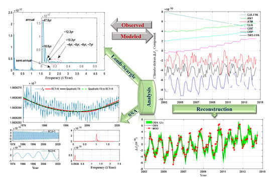
This study analyzes the geophysical signals in J₂ time series from 1976 to 2020 by using singular spectrum analysis (SSA) and the Lomb-Scargle (L-S) periodogram for the first time. The results of SSA indicate that the secular trend is characterized by a superposition of the secular linear decrease with a rate of approximately (−5.80 ± 0.08) × 10⁻¹¹/yr and an obvious quadratic rate of (2.38 ± 0.02) × 10⁻¹³/yr². Besides, the annual, semi-annual, and 10.6-year signals with determining for the first time its amplitude of 5.01 × 10⁻¹¹, are also detected by SSA, where their stochastic behavior can be maintained to the greatest extent. The 18.6-year signal cannot be detected by SSA even when the window size of 18.6 years was selected, while L-S periodogram can detect the signal of 18.6 years after removing the 18.6-year tidal theoretical value and the linear trend, proving the existence of the tidal variations of 18.6 years in the residual time series. Nevertheless, the 10.6-year signal can be found only after removing the secular trend. This fact suggests that the advantages of different methods used will lead to different sensitivity to the particular signals hard to be detected. Finally, the reconstructed ΔJ₂ time series through the sum of the climate-driven contributions from glacial isostatic adjustment (GIA), Antarctic ice sheets (ANT), atmosphere (ATM), continental glaciers (GLA), Greenland ice sheets (GRE), ocean bottom pressure (OBP), and terrestrial water storage (TWS) by using GRACE gravity field solution and geophysical models agrees very well with that of the observed ΔJ₂ from SLR in terms of the amplitude and phase. About 81.5% of observed ΔJ₂ can be explained by the reconstructed value. ATM, TWS, and OBP are the most significant contributing sources for seasonal signals in ΔJ₂ time series, explaining up to 40.1%, 31.9%, and 26.3% of the variances of observed ΔJ₂. These three components contribute to the annual and semi-annual variations of the observed ΔJ₂ up to 30.1% and 1.6%, 30.8% and 1.0%, as well as 25.4% and 0.7%, respectively. GRE, ANT, and GLA have ~3 to ~7-year periodic fluctuations and a positive linear trend, excluding GIA.

1. Introduction

The accurate recovery and analysis of the Earth’s oblateness term C₂₀ (or J₂) time series are of great significance for understanding the mass redistribution in the Earth’s climate system [1,2]. Since 1976, the C₂₀ time series derived from the satellite laser ranging (SLR) observations to geodetic satellites by Cheng and Ries [2] from the Center of Space Research (CSR) has been of the highest quality, even though various research institutes have recently taken their efforts to the SLR-derived, GRACE-derived (Gravity Recovery and Climate Experiment satellite mission) or SLR-GRACE-derived C₂₀ time series, such as the Astronomical Institute, University of Bern (AIUB) [3], the Deutsches Geodätisches Forschungsinstitut, Technische Universität München (DGFI) [4], the NASA Goddard Space Flight Center (GSFC) [5] and the Centre National d’Etudes Spatiales/Groupe de Recherche de Géodésie Spatiale (GRGS) [6]. GRACE is less sensitive to the zonal harmonics, in particular J₂ [7], because of its near-polar orbit inclination (89.3°). Though the GRACE-derived C₂₀ has been greatly improved with the improvement of solution strategies and force models in recent years, it is not as reliable as SLR estimates [7] and should be replaced by SLR-derived C₂₀ for scientific interpretations and geophysical applications of GRACE and GRACE-FO data products. In this paper, the time-variation characteristics of the SLR-derived C₂₀ time series from CSR [1,2] are intensively analyzed.

During the past four decades, various analyses of SLR data have indicated that the mass redistribution within the Earth’s dynamic system has been undergoing significant variations as a response to the tidal and non-tidal changes ranging from hours to decades or longer-periods [2,8], which is characterized by the temporal variations in the Earth’s gravity field. The surface mass redistribution concentrated in a thin layer on the Earth’s surface is reflected by the variations of the spherical harmonic (SH) coefficients of the Earth’s gravity field model. C₂₀ is the largest SH coefficient, which is often described instead of J₂ with a relationship of $J_2=-\sqrt{5}{C}_{20}$. J₂ is called the Earth’s oblateness and its variation is at the magnitude of 10⁻¹⁰.

In the previous studies, the variations of J₂ have been routinely characterized by the following model

$$\Delta J_2=\Delta J_2\left(t_0\right)+\dot{J_2}\left(t-t_0\right)+\frac{1}{2}\ddot{j_2}{\left(t-t_0\right)}^2+\Delta J_2^{NT}\left(t\right)+\Delta J_2^T\left(t\right)$$

It is the superposition of a secular trend and accelerations ($\dot{J_2}$and $\ddot{j_2}$), tidal ($\Delta J_2^T\left(t\right)$) and non-tidal variations ($\Delta J_2^{NT}\left(t\right)$) [1,2]. $\Delta J_2^T\left(t\right)$ and $\Delta J_2^{NT}\left(t\right)$ are typically described by seasonal variations, interannual variations, decadal variations, and longer-period variations [2,9]. Since 1976, Cheng and Ries [2], Cheng et al. [1], Cheng and Tapley [10], and other researchers [9,11,12,13,14,15] have studied the J₂ time series as its time-span increases year by year, understanding the nature of the secular trend of J₂, from a linear trend by analyzing a short time series [10,16,17] or a long time series of more than three decades employing a quadratic trend [1,2,7,9,13,15]. Cheng et al. [1] characterized the nature of the secular trend by a quadratic curve imposed on a period tidal signal of 18.6 years. The quadratic term is described by the superposition of a linear decrease induced by glacial isostatic adjustment (GIA) or postglacial rebound (PGR) of the Earth’s mantle [11,18,19] and a slowly increasing rate caused by global mass redistribution related to the ice-sheet and glacial melting as well as mass transfer in the atmosphere and ocean [2]. Other effects are also considered as factors influencing the oblateness changes, such as co-seismic effects induced by earthquakes [20,21], artificial water reservoir impoundment [22], and the Earth’s spin-down, induced by the tidal forcing [23] which contributes to the deceleration of J₂ at the order of 10⁻¹²/yr. The global sea-level rise enlarges the above rate by almost the same value. The different secular decrease rates of the Earth’s oblateness have been reported by analyzing the SLR data covering different time intervals from 5 years up to four decades, where the first secular decrease is −3 × 10⁻¹¹/yr [12], then −2.6 × 10⁻¹¹/yr derived from 10-year data after 1980 and −2.8 × 10⁻¹¹/yr from 1976 to 1995 [24], −1.95 × 10⁻¹¹/yr from 1980 to 1998 [15], −2.75 × 10⁻¹¹/yr from 1976 to 2004 [10], −5.9 × 10⁻¹¹/yr from 1976 to 2010 by considering it to be a quadratic curve [1].

In addition to the well-known annual and semiannual variations of J₂, the interannual variations related to the strong EI Nino-Southern Oscillation (ENSO) [10,25] generally with the fluctuations of 4 to 6 years were reposted. “The 1998 anomaly” described by Cox and Chao [15] has drawn significant attention and is believed to be caused by the mass redistribution associated with the atmosphere, ocean, and land water [1]. Besides the interannual period, the decadal variations of 18.6 years and about 10.5 years are the evident signals from the analysis of Cheng and Ries [2]. The period of 18.6 years is a pure tidal harmonic signal, while the possible cause and nature of the variation of about 10.5 years with variable amplitude and phase related to climate change remain unknown. Previous studies [1,2,15] indicated that, apart from the tidal harmonic and linear variations, J₂ variation presents an obvious climate-related nonharmonic behavior, especially the varying amplitude and phase. To process these signals, a variety of methods were used. Cheng and Tapley [1,15] adopted the wavelet analysis to decompose ΔJ₂ into high- and low-frequency, where the discrete approximation of the Meyer wavelet is applied as a low pass filter and a sliding average of 360 days is used as a high pass filter, analyzing the long-term variations and removing the seasonal and high-frequency variations in J₂, respectively. Chao et al. [9] subtracted the quadratic trend and seasonal signals with a constant amplitude from ΔJ₂ by using the least-squares fit, ignoring the stochastic behavior of these signals. Cheng and Ries [2] detected the evident variation of 18.6 years in the original ΔJ₂ time series by using Meyer wavelet, whereas Ding and Chao [26] and Chao et al. [9] presented a quite small signal of 18.6-year by using the stabilized AR-𝔃 spectrum (autoregressive spectrum implemented in the complex 𝔃 domain) after removing the linear variation and 18.6-year tidal theoretical value. However, Seo et al. [13] failed to find this ~18.6-year signal in the residual time series. Cheng and Ries [2] explained that the lack of this signal in the analysis of Seo et al. [13] is attributed to the 11-month sliding average used. Therefore, the existence of the 18.6-year signal from the analysis of different methods has led to different discussions.

Singular spectrum analysis (SSA) is a powerful method for studying nonlinear time series. It was first proposed and used by Colebrook [27] in biological oceanography, then introduced into paleoclimatology by Fraedrich [28] and in the study of social issues by Hassani [29]. It can construct and decompose as well as reconstruct a trajectory matrix based on the time series, realizing the accurate separation of principal components, including trend and periodic signals from the remaining component generally regarded as noise [30,31], even when the time series is incomplete [32,33]. The SSA is able to analyze the structure of the time series and make further predictions. As a powerful non-parametric spectrum estimation technique, SSA allows us to effectively follow the evolution in amplitudes and phases of signals [29,34]. As a special application of the empirical orthogonal function, SSA conducts the construction of the principal components of a time series and its prediction by using the w-correlation criterion [29]. Besides, the Lomb-Scargle (L-S) periodogram is well known for detection and characterization of the periodic signals hidden in an unevenly sampled time series and has been widely used in the analysis of astronomical data. The L-S occupies a unique position in various available methods: it is driven by Fourier analysis [35], but it is equivalent to the least-squares method [36]. It can be generated from the principles of Bayesian probability theory [37] and has a close relationship with the bin-based phase folding technology in some cases [38]. As another method, the L-S periodogram holds a unique correspondence point between many types of methods, so we also attempt to analyze the variations of J₂ by using the L-S periodogram in this study.

In addition to the above spectrum analysis, the time series of ΔJ₂ can also be analyzed and reconstructed using geophysical models and other approaches [39]. Many researchers have modeled mass variations of ice sheets, glaciers, terrestrial water, atmosphere, etc., for seeking the geophysical source interpretation in the ΔJ₂ time series. Seo et al. [13] modeled the climate contributions to ΔJ₂, accounting for the relation between the glacial mass change over the Arctic and Alaska and the oscillation of 18.6-year tide. Chao et al. [9] added the theoretical terms (i.e., 18.6-year tide) that Cheng et al. [2] has removed back to ΔJ₂ and modeled the climate-driven sources of Arctic Oscillation, Pacific Decadal Oscillation (PDO), ENSO, etc. for establishing the connections between these sources and the interannual-to-decadal variations of observed ΔJ₂ while Cheng and Tapley [10] validated that the 4- to 6- year fluctuations are related with the PDO and ENSO by geophysical models. Sun et al. [39] improved a new approach related to fingerprints of the geoid changes patterns to estimate ΔJ₂, explaining the residuals by terrestrial water storage after removal of the atmosphere and ocean variations from ΔJ₂. In this study, we analyze the climate-driven components in ΔJ₂ and then conduct the comparison between the reconstructed and observed ΔJ₂ time series, which enables us to gain an in-depth understanding of the geophysical interpretation of J₂ variations.

Therefore, this study mainly focuses on the analysis and interpretation of Earth’s oblateness variations (ΔJ₂) from two different perspectives. One is to analyze the observed ΔJ₂ time series from the perspective of spectrum analysis by applying both SSA and L-S periodogram, respectively; the other is to calculate the contributions of climate-driven components to ΔJ₂ from the perspective of a geophysical model and then analyze the contribution of each component to the observed ΔJ₂ time series and reconstruct the ΔJ₂ time series as well as give the corresponding geophysical interpretation. The rest of the paper is organized as follows. Section 2 briefly presents the theory of SSA and L-S periodogram. Section 3 provides the analysis of the secular trend and periodic signals in J₂ variations and their geophysical interpretation. Section 4 gives a brief introduction of the climate-driven components of ΔJ₂ and the comparison between the reconstructed and observed ΔJ₂. Conclusions are given in Section 5.

2. Analysis Methods

2.1. Singular Spectrum Analysis

By using SSA, the original one-dimensional time series can be decomposed into a sum of constituents. Each component can be determined as either a noise component, a quasi-periodic or periodic component, or a trend component [29]. For a J₂ series $\left\{J_i,i=1,2,\dots ,M\right\}$ with length M, the trajectory matrix $\mathit{J}$ can be formed by a window with size $W$ ($W<M/2$) as follows:

$$\mathit{J}=\left[\begin{array}{cccc}{J}_1& J_2& \cdots & J_{M-W+1}\\ J_2& J_3& \cdots & J_{M-W+2}\\ ⋮& ⋮& \ddots & ⋮\\ J_W& J_{W+1}& \cdots & J_M\end{array}\right].$$

(1)

Then, the covariance matrix ${\mathit{P}}_{\mathrm{J}}$, which has a Toeplitz structure, is expressed as

$${\mathit{P}}_J=\left[\begin{array}{cccc}a(0)& a(1)& \cdots & a(W-1)\\ a(1)& a(0)& \cdots & a(W-2)\\ ⋮& ⋮& \ddots & ⋮\\ a(W-1)& a(W-2)& \cdots & a(0)\end{array}\right]$$

(2)

where the unbiased autocovariance function $a(i)$ is computed by

$$a(i)=\frac{1}{M-i}{\displaystyle \sum _{k=1}^{M-i}{J}_k}{J}_{k+i},i=0,1,\cdots ,W-1$$

(3)

The covariance matrix ${\mathit{P}}_{\mathrm{J}}$ is decomposed as ${\mathit{P}}_{\mathrm{J}}=\mathit{V}\mathit{\Lambda }{\mathit{V}}^{\mathit{T}}$, where $\mathit{\Lambda }$ is a diagonal matrix with the diagonal values ${\lambda }_q$ sorted in descending order and $\mathit{V}$ is an orthogonal matrix with row eigenvectors ${\mathit{v}}_q$. The temporal principal components (PCs) matrix $\mathit{C}$ can be generated as $\mathit{C}=\mathit{V}\mathit{J}$ after projecting the series $J_i$ onto ${\mathit{v}}_q$. The PCs at$k\mathrm{th}$ row and $q\mathrm{th}$column of C is expressed as

$$c_{k,q}={\displaystyle \sum _{i=1}^W{J}_{k+i}}{v}_{i,q}$$

(4)

where $0\le k\le M-W,1\le i\le W$. The$q\mathrm{th}$ Reconstructed Component (RC), which is defined by showing how to optimally extract a series of length M, corresponding to a given set of eigenvalues, can be given by

$$J_{k,q}=\{\begin{array}{cc}\frac{1}{k}{\displaystyle {\sum }_{i=1}^k{c}_{k-i+1,q}{v}_{i,q},}& 1\le k\le W-1\\ \frac{1}{W}{\displaystyle {\sum }_{i=1}^k{c}_{k-i+1,q}{v}_{i,q},}& W\le k\le M-W+1\\ \frac{1}{M-k+1}{\displaystyle {\sum }_{i=k-M+W}^W{c}_{i-k+1,q}{v}_{i,q},}& M-W+2\le k\le M\end{array}$$

(5)

where $J_{k,q}$ is the kth component from the$q\mathrm{th}$PCs. Since ${\lambda }_q$ is sorted in descending order, the first several numbers of RCs can approximate the original time series, while the remaining RCs can be regarded as noise. Therefore, if one wants to reconstruct series ${\widehat{J}}_q$, it can be obtained by the sum of the first q RCs.

The window size is a key issue of SSA and is chosen empirically. The optimal window size should maximize the separation of the contained signals [40] and is usually proportional to the periods of main signals. The window length W is selected to best reflect the separability of SSA. The property ‘separability’ of SSA is also called the weighted correlation or w-correlation [29], which is a natural measure of dependence between two decomposed series $T^{\left(k\right)}$ and $T^{\left(i\right)}$in Equation (6),

$$\begin{array}{cc}{\rho }_{ki}^{(e)}=\frac{(T^{(k)},T^{(i)})}{{\Vert T^{(k)}\Vert }_e{\Vert T^{(i)}\Vert }_e},& (1\le k\le i\le M)\end{array}$$

(6)

where $T^{\left(i\right)}{}_e=\sqrt{{\left(T^{\left(i\right)},T^{\left(i\right)}\right)}_e}$, ${\left(T^{\left(k\right)},T^{\left(i\right)}\right)}_e={\displaystyle \sum }_{q=1}^M{e}_q{t}_q^{\left(k\right)}{t}_q^{\left(i\right)}$,$e_q=min\left\{q,W,M-q\right\}$. The smaller absolute w-correlation value means the worse w-orthogonal of two series, and the zero value indicates that the two series are completely separable. On the contrary, the two series will be far from w-orthogonal and strongly dependent. Therefore, we possibly regard the two PCs with large w-correlation as one periodic signal pair.

2.2. Lomb-Scargle Periodogram Analysis

The L-S periodogram is a well-known technique to attain periodicity by analyzing the frequency spectrum, especially from unequally spaced data [41,42], which is exactly equivalent to the least-squares fitting of a sine wave. In previous studies, it was mainly developed and used in spectral analysis of the unequally sampled astronomical observation. It has the advantage of maintaining the property of the original data and avoiding the interpolation of uneven data. Here, as a special application, we use it to determine the spectrum of equal data.

For the J₂ series $\left\{J_k,k=1,2,\dots ,M\right\}$ with the length M, the discrete Fourier transform for an arbitrarily sampled data set is defined as

$$F(w)={\displaystyle \sum _{k=1}^{M}J(t_k)}{e}^{-iw{t}_k}$$

(7)

Then, the classical periodogram is computed by applying the definition of the Fourier power spectrum, as follows:

$$\begin{array}{l}{p}_J(w)=\frac{1}{M}{\left|F(w)\right|}^2=\frac{1}{M}{\left|{\displaystyle \sum _{k=1}^M{J}_k{e}^{-iw{t}_k}}\right|}^2\\ =\frac{1}{M}\left[{\left({\displaystyle {\sum }_k{J}_k\cos (w{t}_k)}\right)}^2+{\left({\displaystyle {\sum }_k{J}_k\sin (w{t}_k)}\right)}^2\right]\end{array}$$

(8)

A generalized form of the periodogram is addressed by Scargle [42] and Zechmeister and Kürster [43] as

$$P_J(w)=\frac{1}{2}\left\{\frac{{\left[{\displaystyle {\sum }_k{J}_k\cos w(t_k-\tau )}\right]}^2}{{\displaystyle {\sum }_k{\cos }^{2}w(t_k-\tau )}}+\frac{{\left[{\displaystyle {\sum }_k{J}_k\sin w(t_k-\tau )}\right]}^2}{{\displaystyle {\sum }_k{\sin }^{2}w(t_k-\tau )}}\right\}$$

(9)

where $\tau$ is defined to ensure time-shift invariance for each $t_k$ and is computed by

$$\tau =(1/2w){\tan }^{-1}\frac{{\displaystyle {\sum }_k\sin 2w{t}_k}}{{\displaystyle {\sum }_k\cos 2w{t}_k}}$$

(10)

In the least-squares analysis, the shift $\tau$ in Equation (10) is considered by Lomb [41] to orthogonalize the normal equations. Because of the strong connection between least-squares analysis and Fourier analysis, Equation (10) is commonly referred to as the L-S periodogram [43,44].

3. Geophysical Signal Detection from ΔJ₂ Time Series

The J₂ time series from more than 44-year of the satellite laser ranging observations of eight geodetic satellites from 1976 to 2020 derived by Cheng and Ries [2] from the CSR website (http://download.csr.utexas.edu/pub/slr/degree_2/Long_term/C20_Long_Term.txt, accessed on 20 January 2021) has been employed, where the theoretical value of the 18.6-year tide was deducted. Besides the J₂ time series, the monthly time-variable gravity field up to degree and order 3, plus C₄₀, is also co-estimated by using the SLR observations. The J₂ time series and the corresponding uncertainties indicated by the light gray band are shown in Figure 1, exhibiting a superposition of a secular trend and periodic variations and smaller uncertainties after 1992, when observations of two satellites, LAGEOS-2 and Stella, were included.

3.1. Geophysical Signals Detected by Singular Spectral Analysis

For the 44-year J₂ time-series, after the removal of the tidal theoretical value with 542 data points, the selection of the window length W is quite important, which is the only parameter in the SSA technique. On the one hand, if the window length is too short, the periodic signal is not easily separated. On the other hand, since the determination of the appropriate window length depends on preliminary information of the time series and the problem at hand [29], it is generally recommended that the window length should be proportional to the period of the interest but not greater than M/2 [29]. Considering the decadal signals, we mainly focus on signals, such as 10.5 and 18.6 years. Therefore, we select three window lengths with 112 points, 132 points, and 223 points, which correspond to the periodic signals of 9.3, 11.0, and 18.6 years, respectively. To identify periodic signals, we compute the absolute w-correlations of the first 30 reconstructed components (RCs) corresponding to the above three window lengths and show them in Figure 2. The w-correlations, shown in Figure 2a,b, are less separable than those of Figure 2c with the window length $W=223$. In Figure 2c, the absolute w-correlations of RCs (2,3), RCs (5,6), and RCs (7,8) are larger than others, indicating that these pairs are strongly correlated. Moreover, we are also mainly interested in the existence of the 18.6-year signal. Therefore, the window length $W=223$ is most suitable to separate the various periodic signals in the J₂ time-series. The variations in J₂ with a window length of 18.6 years are analyzed for the detection of the various periodic signals.

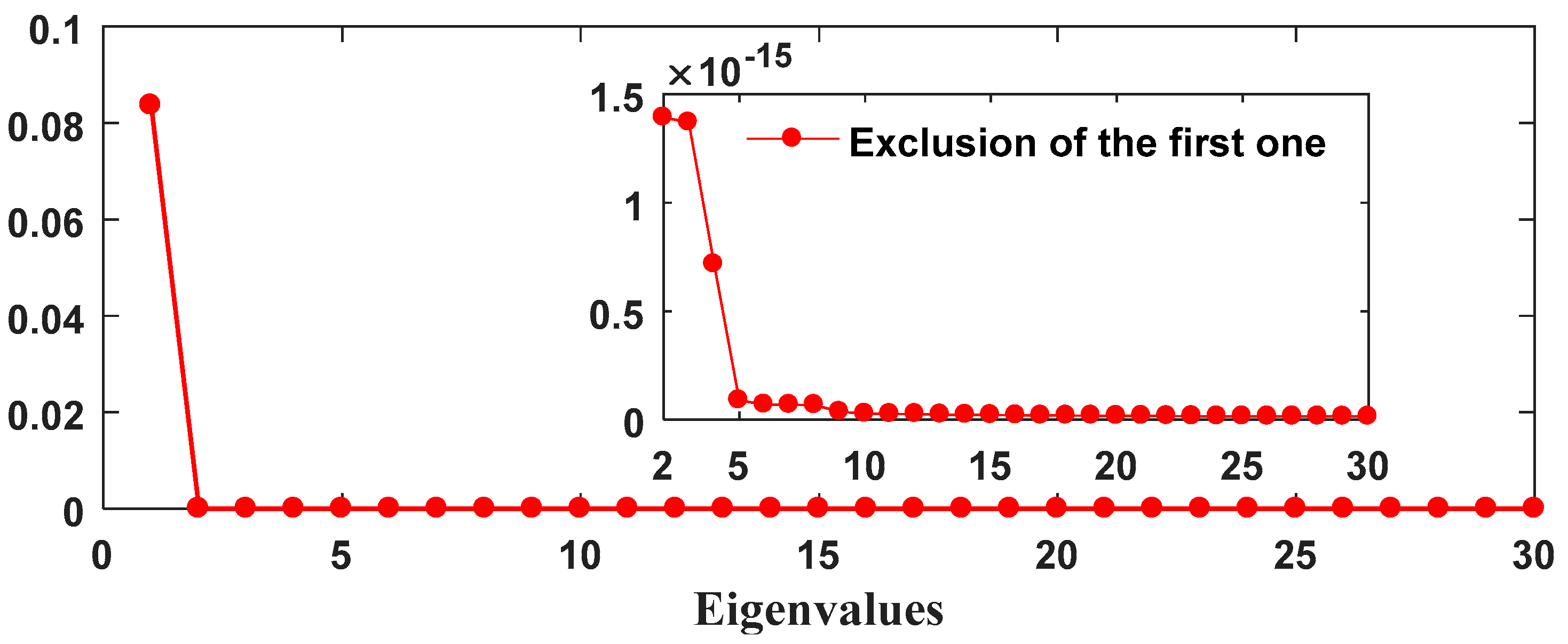
The eigenvalues of the first 30 RCs are illustrated in Figure 3 for the window length $W=223$. The first eigenvalue is much larger than the others, which indicates that RC (1) is much more significant than other components. The first and forth eigenvalues show the general tendency of the J₂ time-series better than the first one alone [29]. Therefore, the RCs (1,4) represents the trend with the red solid line, as illustrated in Figure 4. By using the quadratic polynomial fitting to the red solid line (in green dotted line) and directly to the J₂ time-series (in black solid line), the derived secular linear decrease rate of about (−5.80 ± 0.08) × 10⁻¹¹/yr and obvious acceleration rate of about (2.38 ± 0.02) × 10⁻¹²/yr² are consistent with the values of −5.90 × 10⁻¹¹/yr and 1.80 × 10⁻¹³/yr² reported by Cheng et al. [1], as listed in

Table 1. The trend in J₂ detected by SSA with a window length of 18.6 years.

RC-Index	Linear Trend Term	Quadratic Term	Time Span
RC (1,4)	(−5.80 ± 0.08) × 10−11/yr	(2.38 ± 0.02) × 10−12/yr2	1976.01~2020.09
Quadratic Fit	(−5.64 ± 0.66) × 10−11/yr	(2.29 ± 0.14) × 10−12/yr2	1976.01~2020.09
Cheng et al. (2013)	−5.90 × 10−11/yr	1.80 × 10−12/yr2	1976.01~2011.01

. Moreover, the evolution of the trend of the J₂ time-series can be better characterized with the solid red line compared to the black solid line, as shown in Figure 4, indicating that the trend derived by SSA has better performance than that from quadratic polynomial. This quadratic trend is attributed to solid Earth’s response to the mass redistribution due to recent significant ice melting [2,5,9,13,45,46].

Besides, the second and third components, the fifth and sixth components, the seventh and eighth components have close eigenvalues at their respective order of magnitude. Thus, RCs (2,3), RCs (5,6), and RCs (7,8) are three pairs of periodic signals. Their characteristics are shown in Figure 4 in detail. Applying the Fast Fourier Transform analysis, we can determine the amplitudes and periods of the three pairs of signals which are the annual, 10.6-year, and semi-annual signals. The annual signal has a much larger amplitude than the 10.6-year and semi-annual signals. As illustrated in Figure 4 and

Table 2. The periodic signals in J₂ detected by SSA with a window length of 18.6 years.

RC-Index	Period	Frequency (1/year)	Amplitude
RC (2 + 3)	annual	1	2.67 × 10−10
RC (5 + 6)	10.6-year	0.0938	5.01 × 10−11
RC (7 + 8)	Semi-annual	2	5.56 × 10−11

, the amplitude of the annual signal is almost five times larger than those of 10.6-year and semi-annual periods.

3.2. Geophysical Signals Detected by Lomb-Scargle Periodogram

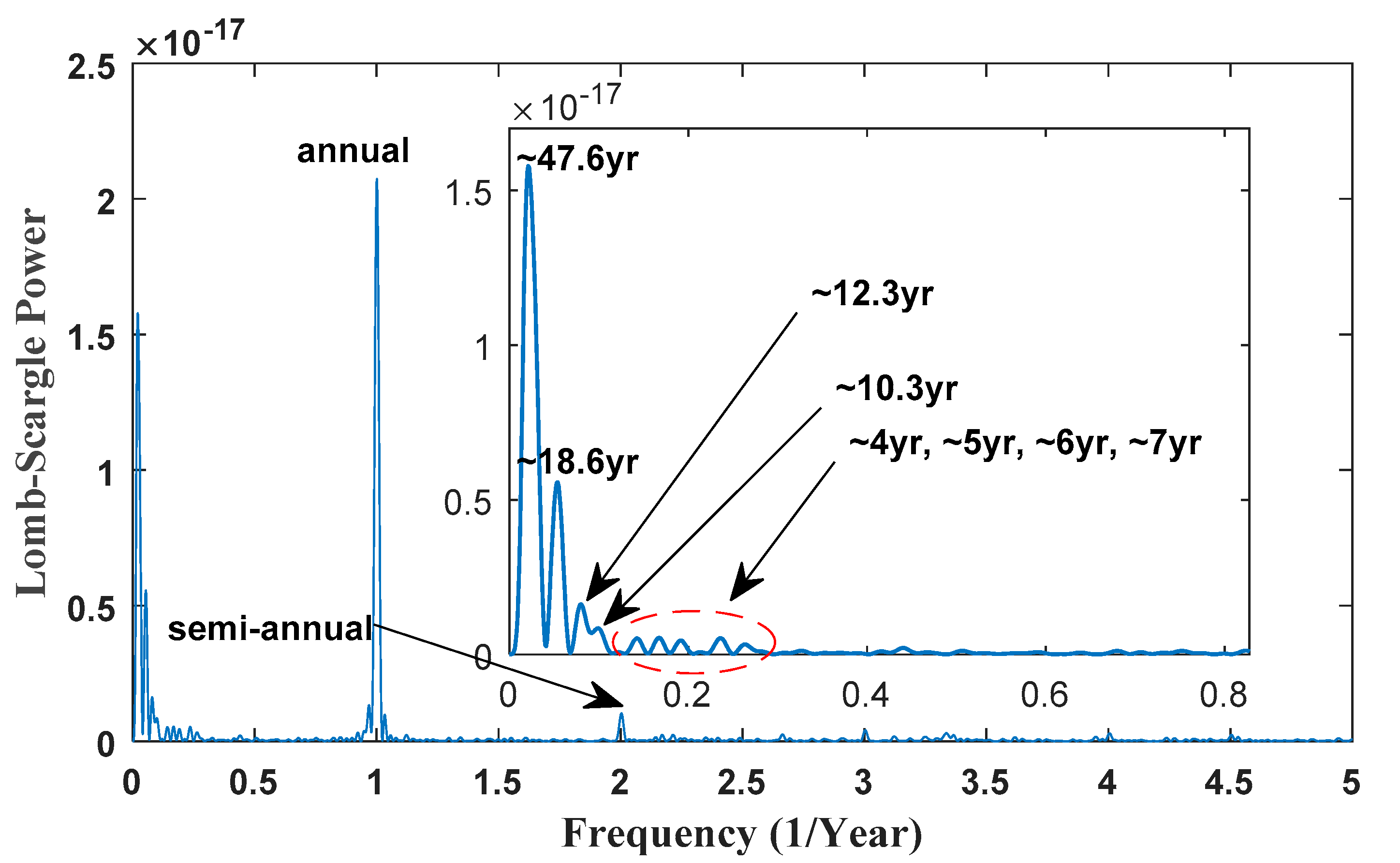
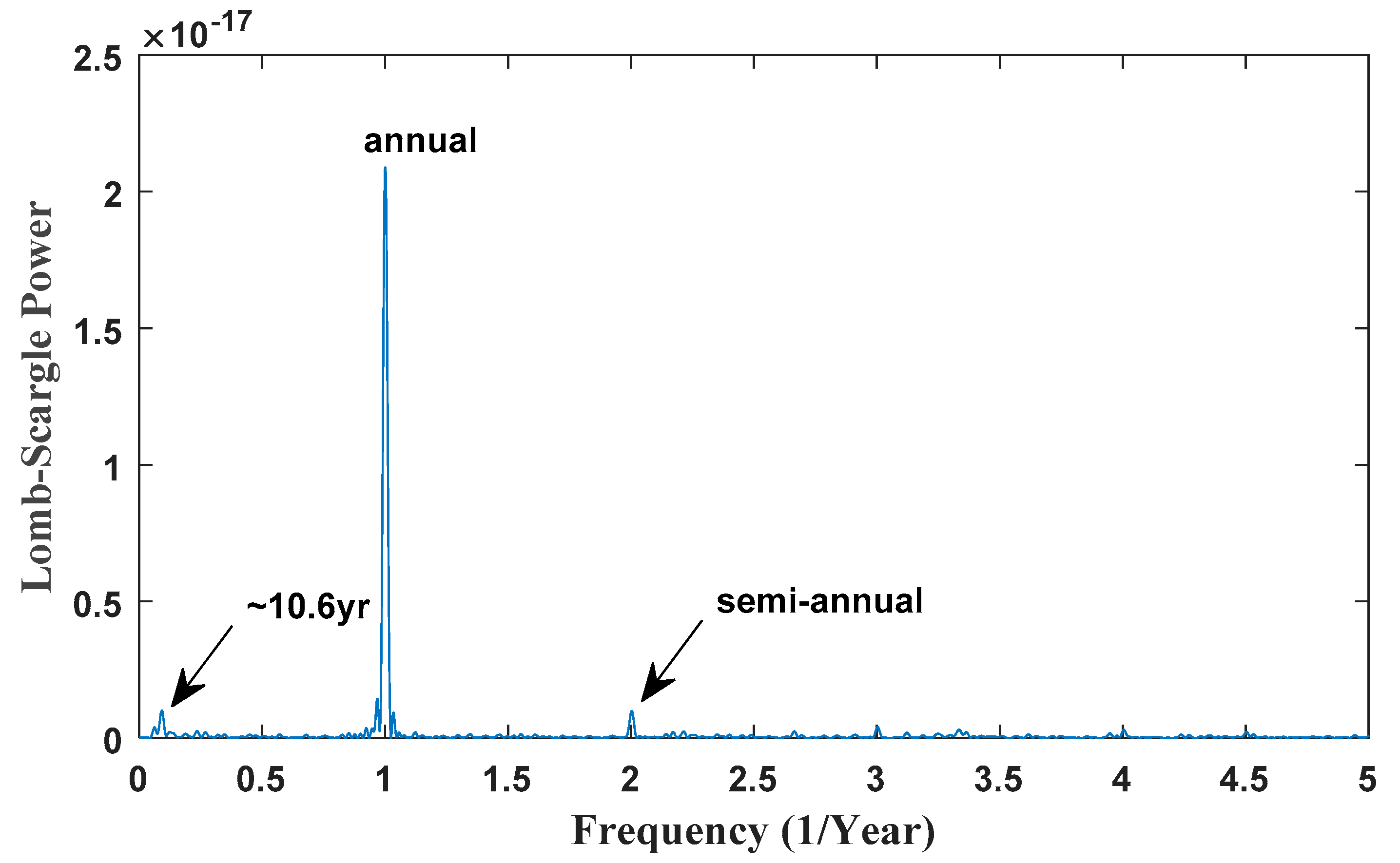
L-S periodogram, as a widely analysis tool used for the astronomical observation, has the simplest statistical behavior, which is important to assess the reliability of the possible detection, and is believed to distinguish between the strictly periodic and nonperiodic signals [42,43]. In addition, the study by Reegen [47] indicates that L-S is based on the identification of the highest peak in a chosen frequency interval, while discrete Fourier transform suffers from systematic deviations of peak frequencies [48]. Reegen [47] also elaborates that L-S is more stable against aliasing and shows improved frequency accuracies than Fourier transform. In this study, the L-S periodogram, is applied for the first time to further analyze the Earth’s oblateness variation after the removal of the tidal theoretical value. The L-S periodograms of the observed ΔJ₂ time series after removing a linear trend and after removing the secular trend with the frequencies from 0 to 5 cycles per year are illustrated in Figure 5 and Figure 6, respectively.

Apart from the significant annual signal, the semi-annual signal and the interannual fluctuations from 4 to 7 years are also detectable in Figure 5. Using this method, a quite small tidal signal with a period of 18.6-year can be detected from the residual time series after removing the 18.6-year theoretical tidal signal and the linear trend from the time series, which was also found by Ding and Chao [26] when the AR-𝔃 spectrum was analyzed. Unfortunately, the signal of 10.5 years cannot be found, while a broadband signal with a peak of approximately 12 years is visible. The peak of 47.6 years in Figure 5 cannot be reasonably explained since it is very challenging to determine whether there is power at wavelengths near the length of the time series (44 years in this paper). For similar reason, no clear explanation can be made by Ding and Chao [26] for the cause of the nominal ~56-year peak shown in the time series from 1976 to 2019. The peak of 47.6 years may be from the artificial signal, which is probably attributed to the sensitivity of the used method to the signal hard to be detected and may explain why different methods show varying abilities to detect some particular signals. According to Cheng et al. [1] and as shown in Figure 1, the Lomb-Scargle periodogram is implemented to the ΔJ₂ time series after removing the secular trend. The signal of 10.6 years is obvious, and the peak of 47.6-year disappears in Figure 6, indicating that the 47.6-year signal may be part of the secular term. Besides, the disappearance of the 18.6-year signal verified Cheng Minkang’s description [1] that the nature of the secular trend is characterized by a quadratic term imposed on a period tidal signal of 18.6 years. In this case, the L-S method does have an advantage over the Fourier transform in detecting the weak 18.6-year signal, which is the same as Chao’s research on finding this 18.6-year signal in the de-linear ΔJ₂ time series [9]. However, the Fourier transform cannot find this signal.

3.3. Discussions

Cheng and Ries [2] detected the dominant period of about 10.4 years from the J₂ time-series, Cheng and Tapley [10] and Seo et al. [13] found a similar period of 10.6 years based on wavelet decomposition, which is determined with the amplitude of 5.01 × 10⁻¹¹ in this study using SSA. Seo et al. [13] also showed that solar activity, measured by the number of sunspots, varies for about 11 years, by comparing the modeled J₂ time series and the number of sunspots from 1979 to 2010. Chao et al. [9] suggested a relationship between the solar cycle and climate change by analyzing the wavelet spectrum of the sunspot variations with 10.5 years. Because solar radiation pressure is quite stable in a solar cycle, it is unlikely that solar activity will directly affect the SLR solutions via the variations in solar radiation pressure [13]. The more acceptable explanation may be that solar activity somehow affects the redistribution of atmospheric or water mass by altering climate change or other unknown causes, which are not included in climate models. Consequently, the causes of 10 years variation still need to be further investigated, as well as convincing observations to understand the effects of the solar activities on climate change and the global gravity field variations.

Although the ΔJ₂ time series may contain the dominant effects of the 18.6-year tide related to the nutation and Earth–Moon tidal interactions [2] which may be a cause of multiyear variations [10], Cheng and Ries [2] found a significant signal of 18.6 years before removal of the 18.6-year tide from the ΔJ₂ time series. Although the residual tidal signal of 18.6 years in the ΔJ₂ time series becomes quite small after the theoretical values are removed, it is still expected to be detected in the analysis of Ding and Chao. In this paper, we get the same results of the small residual tidal signal of 18.6 years using the L-S periodogram. However, we cannot find this signal using the SSA approach, even if adopting the length window of 18.6 years, which is the same as that of Seo et al. [13].

4. Reconstruction and Interpretation of the Variations in the Earth’s Oblateness

4.1. ΔJ₂ Reconstruction with Climate-Driven Sources

Variations in J₂, due to changes in surface mass density ($\Delta {\sigma }_0(\theta ,\lambda ,t)$), can be computed by [11]:

$$\Delta J_2(t)=-\frac{1+k_2}{5}\frac{R^2}{M}{\displaystyle \int \Delta {\sigma }_0(\theta ,\lambda ,t)P_2}(\cos \theta )dS$$

(11)

where k₂ is the Earth’s load Love number for degree 2; M denotes the Earth’s mass and R is the Earth’s mean radius; $\theta$, $\mathsf{\lambda }$, t and $P_2\left(\cos \theta \right)$ are the colatitude, longitude, time and the Legendre polynomial, respectively.

In this study, we derive contributing sources of ΔJ₂ including Antarctic (ANT) and Greenland (GRE) ice sheets, atmosphere (ATM), ocean bottom pressure (OBP) as well as continental glaciers (GLA) by using the geophysical models for the first time, similar to the research of geocenter motion by Zhang and Sun [49]. Readers can refer to Zhang and Sun [49] and the appendix of this study for detailed information of the adopted geophysical models. However, models for terrestrial water storage (TWS) and glacial isostatic adjustment (GIA) still have large uncertainties. Therefore, in a way different from that in Zhang and Sun [49], we take solutions from Sun et al. [39,50,51,52] that estimates contributing sources of ΔJ₂ including TWS and GIA using GRACE data combined with a suitable set of fingerprints (fingerprints approach, FPA) covering the period Jan. 2003 to Jun. 2014. As a novel way to interpret temporal variations of the Earth’s gravity field, FPA was proposed by Rietbroek et al. [53] and improved by Sun et al. [39] (refer to Appendix A).

4.2. Comparison and Interpretation of Reconstructed and Observed ΔJ₂

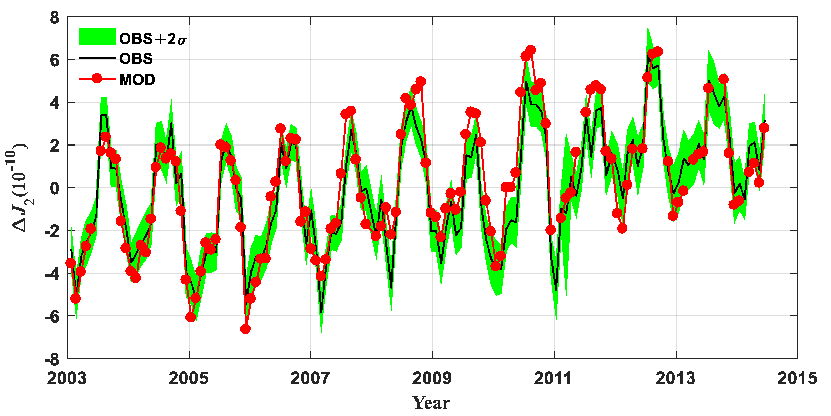
Figure 7 shows seven climate-driven ΔJ₂ components. ATM, OBP, and TWS significantly contribute to seasonal signals in ΔJ₂, while GIA, ANT, GLA, and GRE mainly influence the linear trend in ΔJ₂. Due to ice melting, ANT, GLA, and GRE are all characterized by a positive linear trend. As an ongoing response of the solid Earth to the past glaciations [15,54], GIA is dominated by a negative trend. We then reconstructed ΔJ₂ by summing all climate-driven components and comparing them to the observed ones for the period January 2003 to June 2014 (Figure 8). The reconstructed ΔJ₂ is markedly in line with that of the observed value from SLR in terms of the linear trend and the amplitude and phase of the annual term, as shown in

Table 3. Annual variations in the observed and reconstructed ΔJ₂ time series.

	Linear Trend	Annual		Semi-Annual		Correlation
		Amplitude	Phase	Amplitude	Phase
OBS	(3.81 ± 0.75) × 10−11/yr	(2.79 ± 0.36) × 10−10	204.6 ± 7.4			92%
MOD	(3.34 ± 0.65) × 10−11/yr	(2.91 ± 0.31) × 10−10	202.1 ± 6.1
GIA	(−2.78 ± 0.00) × 10−11/yr
ANT	(1.62 ± 0.04) × 10−11/yr
GLA	(1.69 ± 0.01) × 10−11/yr
GRE	(2.80 ± 0.07) × 10−11/yr
TWS	(1.07 ± 0.40) × 10−11/yr	(1.01 ± 0.19) × 10−10	203.2 ± 10.8	(3.75 ± 0.90) × 10−11	206.0 ± 14.3
ATM		(0.89 ± 0.20) × 10−10	199.0 ± 13.0	(1.61 ± 0.49) × 10−11	188.1 ± 17.8
OBP		(0.83 ± 0.14) × 10−10	201.3 ± 9.8	(1.51 ± 0.41) × 10−11	186.2 ± 16.0

and Figure 8. We employ the SSA method, as described in Section 2.1 and Section 3.1 to extract the annual and semi-annual signals of ATM, OBP and TWS for the analysis of their amplitudes and phases, while the trends for GIA, ANT, GLA and GRE are calculated. The absolute values of the trends of GIA and GRE are equivalent, and ANT and GLA have the same positive trend. The annual amplitude of TWS is slightly larger than those of ATM and OBP with almost the same phase, while the semi-annual amplitude of TWS is almost twice as large as the other two components.

In addition, the variance V of the observed ΔJ₂ explained by the reconstructed ΔJ₂ can be calculated according to

$$V=1-\mathrm{var} \langle OBS-{MOD}_X \rangle /\mathrm{var} \langle OBS \rangle$$

(12)

where <> denotes variance operator; X represents reconstruction; OBS and MOD_X represent the observed and reconstructed ΔJ₂, respectively. In order to quantify the contribution of each component to ΔJ₂, the variance of the observed ΔJ₂ explained by each contributing source is calculated when X denotes the component and MOD_X represents the individual contributing component.

The results of the variance V (

Table 4. The variance of the observed ΔJ₂ explained by climate-driven components and the reconstructed ΔJ₂.

Sources	Total	ANT	ATM	GLA	GRE	OBP	TWS
V (%)	81.5	11.0	40.1	13.5	22.6	26.3	31.9
V (%, Annual)			30.1			25.4	30.8
V (%, Semi-annual)			1.6			0.7	1.0

) show that the observed ΔJ₂ is 81.5% explained by the reconstructed solution, suggesting that all the main characteristics of ΔJ₂ have been well explained. In addition, the correlation coefficient between the two time series is 92% (Table 3). Both Antarctica ice sheet and continental glaciers account for less than 15% of the variance of the observed ΔJ₂. Greenland ice sheet has a slightly larger contribution, but still explains less than 25% of the variance. The TWS and atmosphere, on the other hand, are the two largest climate sources causing periodic signals in ΔJ₂, which explain up to 31.9% and 40.1% of the variance of the observed ΔJ₂, respectively. Besides, the results of SSA show that the TWS, ATM and OBP can contribute to the annual and semi-annual variations of the observed ΔJ₂ up to 30.8% and 1.0%, 30.1% and 1.6%, as well as 25.4% and 0.7%, respectively.

The L-S periodogram of the climate-driven components is illustrated in Figure 9 for further interpreting the corresponding climate or geophysical sources of the observed J₂ variabilities. The ATM, OBP, and TWS are the most significant driving sources for annual variation, while they contribute to the semi-annual variations of ΔJ₂ time series in a very small order of magnitude. The peaks at the periods of about 3, 4, 6, and 7 years originate from the mass variations of Greenland and Antarctica ice sheets and continental glaciers, while the OBP makes no contributions to these fluctuations. This fact may imply that the strong ENSO [10] with 4- to 7-year fluctuations leads to the mass variations of Greenland and Antarctica ice sheets and continental glaciers to alter J₂. However, ENSO has no impact on OBP and the 4–7-year signals in GIA could be artificial, resulting from the L-S periodogram. Besides, it is noteworthy that TWS dominates an evident period of 12.2-year, which could either probably explain the existence of this periodic signal in Figure 5, but a further study may be needed. Due to the short ΔJ₂ time series during the GRACE era, those long-period variations cannot be verified.

5. Conclusions

The variations in J₂ reflect the mass redistributions within the Earth system, routinely characterized by a superposition of a secular trend, seasonal variations, interannual variations, decadal variations, and longer-period variations. ΔJ₂ of more than 44 years from 1976 to 2020 is analyzed by SSA and L-S for the first time. The results show that the secular linearly decreases a rate of approximately (−5.80 ± 0.08) × 10⁻¹¹/yr and an obvious quadratic rate of (2.38 ± 0.02) × 10⁻¹³/yr² derived from SSA is consistent with the results from Cheng et al. [1] by quadratic polynomial fitting. Besides the seasonal variations, the variations at the ~10.6-year period, related to the solar activities, can be notably detected, determining its amplitude of 5.01 × 10^–11 for the first time, whereas there is no 18.6-year periodic signal after removal of the theoretical tidal value from J₂ even if the 18.6-year window size is selected by applying SSA. However, in the spectrum analysis of L-S, the 18.6-year periodic variations and ~3 to ~6-year fluctuations are all detectable in the de-linear time series. This fact suggests that the advantages of different methods used will lead to different sensitivity to the particular signals that are hard to detect. SSA can maintain the stochastic behavior of the signals it separated to the greatest extent, while small long-period signals can be detected in the spectrum analysis of L-S.

In any case, the ΔJ₂ time series during the GRACE era is reconstructed based on the geophysical models and FPA by considering the mass variations from GIA, ANT, ATM, GLA, GRE, OBP, and TWS. The reconstructed ΔJ₂, by summing all the climate-driven components, is markedly close to that of the observed ΔJ₂ with a high correlation coefficient of 92%. The reconstructed ΔJ₂ can also explain up to 81.5% of the variance of the observed value. The most significant climate-driven sources for seasonal signals in the ΔJ₂ time series mainly originated from ATM, TWS, and OBP, which explains up to 40.1%, 31.9%, and 26.3% of the variance, respectively. These three components, in total, can account for the annual and semi-annual variations in the observed ΔJ₂, up to 86.3% and 3.3%, respectively. However, GRE, ANT, and GLA dominate the positive linear trend with interannual periodic fluctuations of ~3 to ~7-years and GIA contributes to a large negative trend.

References

1. Cheng, M.; Tapley, B.D.; Ries, J.C. Deceleration in the Earth’s oblateness. J. Geophys. Res. Solid Earth 2013, 118, 740–747. [Google Scholar] [CrossRef]
2. Cheng, M.; Ries, J.C. Decadal Variation in Earth’s Oblateness (J2) from Satellite Laser Ranging Data. Geophys. J. Int. 2018, 212, 1218–1224. [Google Scholar] [CrossRef]
3. Sośnica, K.; Jäggi, A.; Meyer, U.; Thaller, D.; Beutler, G.; Arnold, D.; Dach, R. Time Variable Earth’s Gravity Field from SLR Satellites. J. Geod. 2015, 89, 945–960. [Google Scholar] [CrossRef] [Green Version]
4. Bloßfeld, M.; Müller, H.; Gerstl, M.; Štefka, V.; Bouman, J.; Göttl, F.; Horwath, M. Second-Degree Stokes Coefficients from Multi-Satellite SLR. J. Geod. 2015, 89, 857–871. [Google Scholar] [CrossRef]
5. Loomis, B.D.; Rachlin, K.E.; Luthcke, S.B. Improved Earth Oblateness Rate Reveals Increased Ice Sheet Losses and Mass-Driven Sea Level Rise. Geophys. Res. Lett. 2019, 46, 6910–6917. [Google Scholar] [CrossRef]
6. Lemoine, J.M.; Bourgogne, S.; Biancale, R.; Bruinsma, S. RL04 Monthly Gravity Field Solutions from CNES/GRGS. In Proceedings of the GRACE/GRACE-FO Science Team Meeting, Potsdam, Germany, 9–11 October 2018; Available online: http://presentations.copernicus.org/GSTM-2018-42_presentation.pdf (accessed on 11 January 2021).
7. Cheng, M.; Ries, J. The Unexpected Signal in GRACE Estimates of C20. J. Geod. 2017, 91, 897–914. [Google Scholar] [CrossRef]
8. Cheng, M.; Ries, J.C.; Tapley, B.D. Variations of the Earth’s figure axis from satellite laser ranging and GRACE. J. Geophys. Res. Space Phys. 2011, 116. [Google Scholar] [CrossRef] [Green Version]
9. Chao, B.F.; Yu, Y.; Chung, C.H. Variation of Earth’s Oblateness J 2 on Interannual-to-Decadal Timescales. J. Geophys. Res. Solid Earth 2020, 125, e2020JB019421. [Google Scholar] [CrossRef]
10. Cheng, M.; Tapley, B.D. Variations in the Earth’s oblateness during the past 28 years. J. Geophys. Res. Space Phys. 2004, 109. [Google Scholar] [CrossRef]
11. Dickey, J.O.; Marcus, S.L.; De Viron, O.; Fukumori, I. Recent Earth Oblateness Variations: Unraveling Climate and Postglacial Rebound Effects. Science 2002, 298, 1975–1977. [Google Scholar] [CrossRef] [PubMed]
12. Yoder, C.F.; Williams, J.G.; Dickey, J.O.; Schutz, B.E.; Eanes, R.J.; Tapley, B.D. Secular Variation of Earth’s Gravitational Harmonic J2 Coefficient from Lageos and Nontidal Acceleration of Earth Rotation. Nat. Cell Biol. 1983, 303, 757–762. [Google Scholar] [CrossRef]
13. Seo, K.-W.; Chen, J.; Wilson, C.R.; Lee, C.-K. Decadal and Quadratic Variations of Earth’s Oblateness and Polar Ice Mass Balance from 1979 to 2010. Geophys. J. Int. 2015, 203, 475–481. [Google Scholar] [CrossRef]
14. Mitrovica, J.X.; Peltier, W.R. Present-Day Secular Variations in the Zonal Harmonics of Earth’s Geopotential. J. Geophys. Res. Space Phys. 1993, 98, 4509–4526. [Google Scholar] [CrossRef]
15. Cox, C.M.; Chao, B.F. Detection of a Large-Scale Mass Redistribution in the Terrestrial System since 1998. Science 2002, 297, 831–833. [Google Scholar] [CrossRef] [Green Version]
16. Cheng, M.K.; Eanes, R.J.; Shum, C.K.; Schutz, B.E.; Tapley, B.D. Temporal Variations in Low Degree Zonal Harmonics from Starlette Orbit Analysis. Geophys. Res. Lett. 1989, 16, 393–396. [Google Scholar] [CrossRef]
17. Cheng, M.; Tapley, B.D. Seasonal Variations in Low Degree Zonal Harmonics of the Earth’s Gravity Field from Satellite Laser Ranging Observations. J. Geophys. Res. Space Phys. 1999, 104, 2667–2681. [Google Scholar] [CrossRef]
18. Ivins, E.R.; Sammis, C.G.; Yoder, C.F. Deep Mantle Viscous Structure with Prior Estimate and Satellite Constraint. J. Geophys. Res. Space Phys. 1993, 98, 4579–4609. [Google Scholar] [CrossRef]
19. Jacob, T.; Wahr, J.M.; Pfeffer, W.T.; Swenson, S.C. Recent Contributions of Glaciers and Ice Caps to Sea Level Rise. Nat. Cell Biol. 2012, 482, 514–518. [Google Scholar] [CrossRef] [PubMed]
20. Xu, C.Y.; Chao, B.F. Seismic Effects on the Secular Drift of the Earth’s Rotational Pole. J. Geophys. Res. Solid Earth 2019, 124, 6092–6100. [Google Scholar] [CrossRef]
21. Chao, B.F.; Ding, H. Global Geodynamic Changes Induced by All Major Earthquakes, 1976–2015. J. Geophys. Res. Solid Earth 2016, 121, 8987–8999. [Google Scholar] [CrossRef]
22. Chao, B.F. Anthropogenic Impact on Global Geodynamics Due to Reservoir Water Impoundment. Geophys. Res. Lett. 1995, 22, 3529–3532. [Google Scholar] [CrossRef] [Green Version]
23. Chao, B.F.; O’Connor, W.P.; Chang, A.T.C.; Hall, D.K.; Foster, J.L. Snow Load Effect on the Earth’s Rotation and Gravitational Field, 1979–1985. J. Geophys. Res. Space Phys. 1987, 92, 9415–9422. [Google Scholar] [CrossRef] [Green Version]
24. Cheng, M.K.; Shum, C.K.; Tapley, B.D. Determination of Long-Term Changes in the Earth’s Gravity Field from Satellite Laser Ranging Observations. J. Geophys. Res. Space Phys. 1997, 102, 22377–22390. [Google Scholar] [CrossRef]
25. Marcus, S.L.; Dickey, J.O.; Willis, J.K.; Seitz, F. Earth Oblateness Changes Reveal Land Ice Contribution to Interannual Sea Level Variability. Geophys. Res. Lett. 2009, 36. [Google Scholar] [CrossRef]
26. Ding, H.; Chao, B.F. Application of Stabilized AR-z Spectrum in Harmonic Analysis for Geophysics. J. Geophys. Res. Solid Earth 2018, 123, 8249–8259. [Google Scholar] [CrossRef]
27. Colebrook, J.M. Continuous Plankton Records-Zooplankton and Environment, Northeast Atlantic and North-Sea, 1948–1975. Oceanol. Acta 1978, 1, 9–23. [Google Scholar]
28. Fraedrich, K. Estimating the Dimensions of Weather and Climate Attractors. J. Atmos. Sci. 1986, 43, 419–432. [Google Scholar] [CrossRef]
29. Hassani, H. Singular Spectrum Analysis: Methodology and Comparison. J. Data Sci. 2007, 5, 239–257. [Google Scholar]
30. Shen, Y.; Guo, J.; Liu, X.; Kong, Q.; Guo, L.; Li, W. Long-Term Prediction of Polar Motion Using a Combined SSA and ARMA model. J. Geod. 2018, 92, 333–343. [Google Scholar] [CrossRef]
31. Guo, J.Y.; Gao, W.Z.; Yu, H.J.; Liu, X.; Kong, Q.L.; Chen, X.D. Gravity Tides Extracted from Relative Gravimetric Data with Singular Spectrum Analysis. Chin. J. Geophys. 2018, 61, 3889–3902. [Google Scholar] [CrossRef]
32. Shen, Y.; Peng, F.; Li, B. Improved Singular Spectrum Analysis for Time Series with Missing Data. Nonlinear Process. Geophys. 2015, 22, 371–376. [Google Scholar] [CrossRef] [Green Version]
33. Wang, F.; Shen, Y.; Chen, T.; Chen, Q.; Li, W. Improved Multichannel Singular Spectrum Analysis for Post-Processing Grace Monthly Gravity Field Models. Geophys. J. Int. 2020, 223, 825–839. [Google Scholar] [CrossRef]
34. Vautard, R.; Ghil, M. Singular Spectrum Analysis in Nonlinear Dynamics, with Applications to Paleoclimatic Time Series. Phys. D Nonlinear Phenom. 1989, 35, 395–424. [Google Scholar] [CrossRef]
35. VanderPlas, J.T. Understanding the Lomb-Scargle Periodogram. Astrophys. J. Suppl. Ser. 2018, 236. Available online: https://iopscience.iop.org/article/10.3847/1538-4365/aab766/pdf (accessed on 25 November 2020). [CrossRef]
36. Reimann, J.D. Frequency Estimation Using Unequally-Spaced Astronomical Data; University of California: Berkeley, CA, USA, 1994. [Google Scholar]
37. Bretthorst, G.L. Bayesian Spectrum Analysis and Parameter Estimation. Lecture Notes in Statistics 48; Springer: Berlin, Germany, 1988. [Google Scholar]
38. Swingler, D.N. A Comparison of the Fourier, Jurkevich, and Stellingwerf Methods of Period Estimation. Astron. J. 1989, 97, 280. [Google Scholar] [CrossRef]
39. Sun, Y.; Riva, R.; Ditmar, P.; Rietbroek, R. Using GRACE to Explain Variations in the Earth’s Oblateness. Geophys. Res. Lett. 2019, 46, 158–168. [Google Scholar] [CrossRef] [Green Version]
40. Kondrashov, D.; Shprits, Y.; Ghil, M. Gap Filling of Solar Wind Data by Singular Spectrum Analysis. Geophys. Res. Lett. 2010, 37. [Google Scholar] [CrossRef] [Green Version]
41. Lomb, N.R. Least-Squares Frequency Analysis of Unequally Spaced Data. Astrophys. Space Sci. 1976, 39, 447–462. [Google Scholar] [CrossRef]
42. Scargle, J.D. Studies in astronomical time series analysis. II-Statistical aspects of spectral analysis of unevenly spaced data. Astron. J. 1982, 263, 835–853. [Google Scholar] [CrossRef]
43. Zechmeister, M.; Kürster, M. The Generalised Lomb-Scargle Periodogram-a New Formalism for the Floating-Mean and Keplerian Periodograms. Astron. Astrophys. 2009, 496, 577–584. [Google Scholar] [CrossRef]
44. Gottlieb, E.W.; Wright, E.L.; Liller, W. Optical Studies of UHURU Sources. XI. A Probable Period for Scorpius X-1= V818 Scorpii. Astrophys. J. 1975, 195, L33–L35. [Google Scholar] [CrossRef]
45. Nerem, R.S.; Wahr, J. Recent Changes in the Earth’s Oblateness Driven by Greenland and Antarctic Ice Mass Loss. Geophys. Res. Lett. 2011, 38. [Google Scholar] [CrossRef]
46. Matsuo, K.; Chao, B.F.; Otsubo, T.; Heki, K. Accelerated Ice Mass Depletion Revealed by Low-Degree Gravity Field from Satellite Laser Ranging: Greenland, 1991–2011. Geophys. Res. Lett. 2013, 40, 4662–4667. [Google Scholar] [CrossRef] [Green Version]
47. Reegen, P. SigSpec. Astron. Astrophys. 2007, 467, 1353–1371. [Google Scholar] [CrossRef] [Green Version]
48. Kovács, G. Frequency Shift in Fourier Analysis. Astrophys. Space Sci. 1981, 78, 175–188. [Google Scholar] [CrossRef]
49. Zhang, H.; Sun, Y. Climate-Driven Seasonal Geocenter Motion during the GRACE Period. Acta Geophys. 2018, 66, 223–232. [Google Scholar] [CrossRef] [Green Version]
50. Sun, Y.; Riva, R.; Ditmar, P. Optimizing Estimates of Annual Variations and Trends in Geocenter Motion and J 2 from a Combination of GRACE Data and Geophysical Models. J. Geophys. Res. Solid Earth 2016, 121, 8352–8370. [Google Scholar] [CrossRef] [Green Version]
51. Sun, Y.; Ditmar, P.; Riva, R. Observed Changes in the Earth’s Dynamic Oblateness from GRACE Data and Geophysical Models. J. Geod. 2016, 90, 81–89. [Google Scholar] [CrossRef] [Green Version]
52. Sun, Y.; Ditmar, P.; Riva, R. Statistically Optimal Estimation of Degree-1 and C20 Coefficients Based on GRACE Data and an Ocean Bottom Pressure Model. Geophys. J. Int. 2017, 210, 1305–1322. [Google Scholar] [CrossRef] [Green Version]
53. Rietbroek, R.; Brunnabend, S.-E.; Kusche, J.; Schröter, J. Resolving Sea Level Contributions by Identifying Fingerprints in Time-Variable Gravity and Altimetry. J. Geodyn. 2012, 59–60, 72–81. [Google Scholar] [CrossRef]
54. Peltier, W.R. Constraint on Deep Mantle Viscosity from Lageos Acceleration Data. Nat. Cell Biol. 1983, 304, 434–436. [Google Scholar] [CrossRef]
55. Rignot, E.; Box, J.E.; Burgess, E.; Hanna, E. Mass Balance of the Greenland Ice Sheet from 1958 to 2007. Geophys. Res. Lett. 2008, 35. [Google Scholar] [CrossRef] [Green Version]
56. Zwally, H.J.; Giovinetto, M.B.; Li, J.; Cornejo, H.G.; Beckley, M.A.; Brenner, A.C.; Saba, J.L.; Yi, D. Mass Changes of the Greenland and Antarctic Ice Sheets and Shelves and Contributions to Sea-Level Rise: 1992–2002. J. Glaciol. 2005, 51, 509–527. [Google Scholar] [CrossRef] [Green Version]
57. Frederikse, T.; Riva, R.; Kleinherenbrink, M.; Wada, Y.; Broeke, M.V.D.; Marzeion, B. Closing the Sea Level Budget on a Regional Scale: Trends and Variability on the Northwestern European continental Shelf. Geophys. Res. Lett. 2016, 43, 10864–10872. [Google Scholar] [CrossRef] [PubMed] [Green Version]
58. Van de Berg, W.J.; Medley, B. Brief Communication: Upper-Air Relaxation in RACMO2 Significantly Improves Modelled Interannual Surface Mass Balance Variability in Antarctica. Cryosphere 2016, 10, 459–463. [Google Scholar] [CrossRef] [PubMed] [Green Version]
59. Rignot, E.; Velicogna, I.; Broeke, M.R.V.D.; Monaghan, A.; Lenaerts, J.T.M. Acceleration of the Contribution of the Greenland and Antarctic Ice Sheets to Sea Level Rise. Geophys. Res. Lett. 2011, 38. [Google Scholar] [CrossRef] [Green Version]
60. Marzeion, B.; Leclercq, P.W.; Cogley, J.G.; Jarosch, A.H. Brief Communication: Global Reconstructions of Glacier Mass Change during the 20th Century are Consistent. Cryosphere 2015, 9, 2399–2404. [Google Scholar] [CrossRef] [Green Version]
61. Dee, D.P.; Uppala, S.M.; Simmons, A.J.; Berrisford, P.; Poli, P.; Kobayashi, S.; Andrae, U.; Balmaseda, M.A.; Balsamo, G.; Bauer, P.; et al. The ERA-Interim Reanalysis: Configuration and Performance of the Data Assimilation System. Q. J. R. Meteorol. Soc. 2011, 137, 553–597. [Google Scholar] [CrossRef]
62. Thomas, M. Ocean Induced Variations of Earths Rotation–Results from a Simultaneous Model of Global Circulation and Tides. Ph.D. Thesis, University of Hamburg, Hamburg, Germany, 2002; p. 129. [Google Scholar]
63. Tamisiea, M.E.; Hill, E.M.; Ponte, R.M.; Davis, J.L.; Velicogna, I.; Vinogradova, N.T. Impact of Self-Attraction and Loading on the Annual Cycle in Sea Level. J. Geophys. Res. Space Phys. 2010, 115. [Google Scholar] [CrossRef] [Green Version]
Figure 1. The J2 time-series from 1976 to 2020.
Remotesensing 13 02004 g001
Figure 2. The first 30 w-correlations of RCs, corresponding to the window lengths of (a) 9.3 years, (b) 11 years, and (c) 18.6 years, respectively.
Remotesensing 13 02004 g002
Figure 3. Eigenvalues of the first 30 RCs.
Remotesensing 13 02004 g003
Figure 4. Main merged periodic signals in J2.
Remotesensing 13 02004 g004
Figure 5. Lomb-Scargle periodogram with the frequency from 0 to 5 cycles per year after removing the linear trend.
Remotesensing 13 02004 g005
Figure 6. Lomb-Scargle periodogram with the frequency from 0 to 5 cycles per year after removing the secular trend.
Remotesensing 13 02004 g006
Figure 7. Contributing sources of ΔJ2. Note that the curves are offsite for clarity.
Remotesensing 13 02004 g007
Figure 8. Comparison between the reconstructed (red curve with solid dots) and observed ΔJ2 (black line). The uncertainties (±2σ) of observed ΔJ2 are indicated by the width of the green band.
Remotesensing 13 02004 g008
Figure 9. Lomb-Scargle Periodogram of the climate-driven components in ΔJ2.
Remotesensing 13 02004 g009