Article

Two-Stream Dense Feature Fusion Network Based on RGB-D Data for the Real-Time Prediction of Weed Aboveground Fresh Weight in a Field Environment

1
College of Engineering, Northeast Agricultural University, Harbin 150030, China
2
College of Engineering, Anhui Agricultural University, Anhui 230036, China
*
Author to whom correspondence should be addressed.
Remote Sens. 2021, 13(12), 2288; https://doi.org/10.3390/rs13122288
Submission received: 20 April 2021 / Revised: 29 May 2021 / Accepted: 6 June 2021 / Published: 11 June 2021
(This article belongs to the Special Issue Precision Weed Mapping and Management Based on Remote Sensing)

Abstract

:
The aboveground fresh weight of weeds is an important indicator that reflects their biomass and physiological activity and directly affects the criteria for determining the amount of herbicides to apply. In precision agriculture, the development of models that can accurately locate weeds and predict their fresh weight can provide visual support for accurate, variable herbicide application in real time. In this work, we develop a two-stream dense feature fusion convolutional network model based on RGB-D data for the real-time prediction of the fresh weight of weeds. A data collection method is developed for the compilation and production of RGB-D data sets. The acquired images undergo data enhancement, and a depth transformation data enhancement method suitable for depth data is proposed. The main idea behind the approach in this study is to use the YOLO-V4 model to locate weeds and use the two-stream dense feature fusion network to predict their aboveground fresh weight. In the two-stream dense feature fusion network, DenseNet and NiN methods are used to construct a Dense-NiN-Block structure for deep feature extraction and fusion. The Dense-NiN-Block module was embedded in five convolutional neural networks for comparison, and the best results were achieved with DenseNet201. The test results show that the predictive ability of the convolutional network using RGB-D as the input is better than that of the network using RGB as the input without the Dense-NiN-Block module. The mAP of the proposed network is 75.34% (IoU value of 0.5), the IoU is 86.36%, the detection speed of the fastest model with a RTX2080Ti NVIDIA graphics card is 17.8 fps, and the average relative error is approximately 4%. The model proposed in this paper can provide visual technical support for precise, variable herbicide application. The model can also provide a reference method for the non-destructive prediction of crop fresh weight in the field and can contribute to crop breeding and genetic improvement.

1. Introduction

In the process of weed management, uniform herbicide spraying is currently the most commonly applied weeding method [1]. However, the large-scale use of herbicides has led to the pollution of the natural environment, increased weed resistance, hidden dangers to food security and biodiversity, and many other agricultural and ecological problems [2,3]. This has led to more focused research on precision weed management strategies. In precision weed management, the most commonly used method is to determine the location of weeds through computer vision technology and to apply herbicides to individual weeds [4,5]. However, from the perspective of plant physiology, the dosage of herbicides is closely related to the type of weed and its physiological parameters [6,7,8]. Applying a uniform herbicide dosage does not maximize the use of herbicides, and there is therefore still room for optimization. Herbicides in weeds directly act on the cells of the weeds, affecting cell metabolism and transport functions and eventually killing the weeds [9,10]. The size of weed cells and tissues directly determines the herbicide dosage [6,11]. The aboveground fresh weight is an index that best reflects the size and cell content of plants [12,13], and it is suitable for use as a quantitative index to provide a basis for determining herbicide dosages for real-time variable herbicide spraying. Therefore, the development of a vision system that can detect weeds in real time in complex farmland environments and obtain fresh weight data can change the process of determining precise application doses and has important guiding significance for precise weed management.
The use of visual technology is a rapid and effective method for evaluating the fresh weight of plants. Jiang et al. [14] developed a lettuce weight monitoring system in a plant factory that segmented RGB images and used the number of pixels and the plant weight data to establish a regression equation. Arzani et al. [15] established a regression relationship between fruit diameter and fresh weight. Reyes et al. [16] used Mask R-CNN to segment RGB images to obtain plant characteristics and establish a regression equation between fresh weight and characteristics to obtain the fresh weight of lettuce. The experiment was carried out on a hydroponic growth bed. Mortensen et al. [17] performed 3D point cloud segmentation and obtained the surface area parameters of lettuce for fresh weight prediction. Lee et al. [18] used the 3D point cloud obtained by Kinect for 3D printing and correlated the weight of the cabbage with the amount of material consumed by the 3D printer. The main method used in the current research is to first extract the plant to be predicted from the background, extract the characteristics of the plant and then establish an association with the fresh weight. However, farmland scenes are complex and changeable; the soil background is uneven, the light fluctuates, the weeds in the field overlap each other, and the types, spatial shapes, and growth positions of the weeds differ. It is therefore difficult to extract weeds from complex backgrounds [19,20]. At the same time, the phenotypic information for each plant is extracted as a predictive factor (e.g., measured value [21], leaf area index [22], pixel number [23]) to establish a single linear regression relationship with the fresh weight of the plant; this single-factor approach does not include sufficient information. The fresh weight of weeds is determined not by a single characteristic parameter but by a combination of multiple characteristics. Therefore, it is still difficult to correlate the multidimensional characteristics of weeds with their fresh weight.
Current methods around the extraction of weeds from the background include the use of computer vision techniques and spectral features as the two main directions. This can be effectively distinguished if there is a significant difference in spectral reflectance between the two weeds [24,25,26,27]. However, the use of spectral cameras is often expensive and demanding (illumination) and it is also difficult to distinguish between weeds with similar spectral features. On the other hand, weed identification using visible light images is mainly based on color features, shape features, or texture features [28,29,30,31,32]. Weed detection based on color features uses different weed and crop color thresholds for effective differentiation. However, when faced with similarly colored weeds and crops, it is difficult to distinguish them even with color space conversion [33], especially for large fields with a relatively large number of weed species, and it is relatively difficult to identify each weed species at a granular level. Identification based on shape and texture is also relatively difficult under conditions of overlapping leaves and similar weed shapes, where shape feature templates are susceptible to interference [34,35,36]. The interspecific similarity of weeds to weeds and the similarity of weeds to crops makes it difficult to perform multi-species weed detection using single-function computer vision methods. In this context, deep learning techniques have performed well in the field of image target detection and recognition [37,38,39,40]. CNNs can automatically acquire multiple features in visible images that are effective for target object recognition, are robust for multi-species target detection in complex environments, and have been applied to weed recognition research [41,42,43,44]. The use of CNN technology for weed identification holds good promise.
Weeds are polymorphic, and different types of weeds exhibit different spatial scale information; the same weed may even exist at different spatial scales at different life stages. The use of 2D plane information obtained as RGB images for estimation has limitations, and it is difficult to use this information to accurately describe the spatial stereo information of weeds. As 3D point cloud technology has developed, it has begun to be applied for plant spatial detection. Zhou et al. [45] used 3D point cloud technology to segment soybean plants. Li et al. [46] developed a low-cost 3D plant morphological characterization system. Chaivivatrakul et al. [47] used 3D reconstruction to characterize the morphology of corn plants. Unlike RGB information, 3D point cloud information can provide spatial scale information [48], and it is obviously more advantageous for describing the spatial structure of weeds. 2D or 3D information essentially obtains phenotypic parameters as a single predictor variable for linear regression. Sapkota et al. [49] used canopy cover obtained from UAV imagery to build a regression model with ryegrass biomass. However the single linear model is weakly expressive and may ignore other potential information in the imagery that has an impact on above ground biomass. The convolutional neural network model has unique advantages for addressing nonlinear relationships. Such models can recognize the complex and nonlinear relationship between the input and output of the modelling process [50,51] and automatically learn implicit characteristic information to directly perform nonlinear regression predictions of fresh weight. At present, it is relatively rare to use convolutional neural networks to directly associate 3D information from weeds with their fresh weight.
In this work, to accurately locate weeds and to predict the fresh weight of weeds with different shapes and positions against a complex farmland background, a combination of 3D point cloud and deep learning techniques is explored.
The contributions of this article are as follows:
  • A method of data collection and preprocessing for constructing the fresh weight of different kinds of weeds is proposed.
  • A YOLO-V4 model and a dense fusion network of two-stream features are established for weed detection and fresh weight estimation.
  • The proposed method is tested and analyzed.

2. Data Collection

2.1. Research Area and Objects

To ensure the practical relevance of the study, the study area was a pristine agricultural arable field in Xiangfang Farm, Harbin, China (126°43′34.31″ E, 45°44′29.98″ N). Maize was sown on 4 May 2020 and planted in a flat crop. Herbicide applications were made in two main stages, the first stage was a pre-sowing closure treatment and the second stage was a herbicide application at the stalk stage, with precision-to-target application techniques mainly geared towards the second stage. So after sowing a closed treatment is applied with acetochlor herbicide. After the closure treatment, we selected three weeds with large population sizes in the field for our study. Sonchus arvensis is a perennial herb of the genus Sonchus in the Compositae family. Solanum nigrum is an annual herb in the Solanaceae family. Abutilon theophrasti Medicus is an annual subshrub herb in the Malvaceae family. In the process of collecting these three kinds of weeds, we did not perform any treatment on other weeds in order to maintain the natural state of the farmland. As depth data were used in this study and weed height was an important factor, three different growing heights were selected for the study. Sonchus arvensis grew at relatively low heights, Abutilon theophrasti Medicus at higher heights and Solanum nigrum in the middle of the two.

2.2. Platform and Equipment

The aim of this study was to provide visual support for an accurate variant target spray system. Therefore, an acquisition platform was used for data acquisition to simulate the field application process. The platform is driven by two wheels with adjustable track speed. The differential steering principle is also used to facilitate easier steering in the field [52]. The wheel spacing is adjustable for easy adjustment of the monopoly distance. Two Kinect v2 sensors are mounted under the platform at a height of 0.8 m above the ground. The centers of the two Kinect v2 sensors are 0.7 m apart.
The Kinect v2 sensor is equipped with a 1920 × 1080 resolution camera and a 512 × 424 depth sensor. The field of view of the camera is 70° × 60°, and the detection range is 0.5 to 4.8 m. The distance between the object and the camera plane can be judged by the reflection time of a projected infrared pulse (ToF). Since infrared pulses are disturbed by natural light in an outdoor environment, it will interfere with the work of Kinect v2 and reduce the quality of depth data. We set up a light shield to weaken the effects of the glare, so that some of the light can enter and the RGB can be captured clearly, and so that the depth camera of the Kinect v2 can be used consistently. When selecting the installation height of the equipment, it is necessary not only to ensure the clear imaging of a single weed but also to correspond to the detection range of the Kinect v2 sensor. Chemical weeding is usually performed in the corn field at the 3- to 5-leaf stage. At this time, the height of the corn and weeds is generally not more than 0.3 meters, so 0.8 meters was selected as the installation height of the Kinect v2 sensor in this study.
The weighing equipment is an analytical balance produced by Shanghai Hochoice Company (China) that is accurate to the milligram.

2.3. Collection Method

To establish a one-to-one relationship between a single weed and its fresh weight in an image simultaneously, it is necessary to ensure that the captured image fully conforms to the working state of the weeding robot in the natural environment. The camera height and light fluctuations caused by the platform also need to be considered. Therefore, static single-frame shooting is not possible, and it is necessary to simulate the walking state of the platform on site for dynamic acquisition. In this study, an efficient method for collecting the weed fresh weight data was developed. Figure 1 shows the collection process. We summarize the collection process into four steps:
  • Step A: Before shooting, the staff must first determine the camera’s field of view and underline the camera’s field of view. Two lines, the edge of the camera’s field of view and the position 400 pixels from the edge of the field of view, are established. The area between the two lines is called the label establishment area. After finding the weeds, the weeds are associated with a label, and the weed type and serial number are recorded in the label establishment area. If the weeds are within the same row, they are marked in order from the farthest to the closest label to the camera. If weeds are on the line or in the label establishment area, the weeds will not be recorded, as shown by the red cross in the picture. After the marking is completed, the lines are moved away to avoid affecting the subsequent shooting. At this point, the label establishment area can be distinguished based on the pixels of the captured image. It should be noted that there is no need to mark weeds on the lines or in the label area because this middle area is eventually cut and used to build the data set. Using this data collection method does not cause human interference with the shooting content in the middle area. This ensures that the constructed data set conforms to the natural state. This collection method is also more effective than other methods.
  • Step B: The collection platform contains two Kinect v2 devices that can collect data from two rows at the same time. The movement speed of the platform is 0.3 meters per second, and the Kinect v2 shooting speed is set to 30 fps. The platform moves straight along the trajectory of the established line. The weeds and tags are photographed at the same time to obtain the RGB-D information for the weeds.
  • Step C: After the platform passes, the staff uses destructive methods to obtain the aboveground parts of the weeds, weighs them on an electronic balance, and records the weight on the label. The robot will stop after walking 60 meters and wait for the collector to complete the collection before continuing. This avoids, as far as possible, any increase in the fresh weight of weeds on the ground due to time.
  • Step D: The MapColorFrameToDepthSpace function in Kinect v2 for Windows SDK 2.0 is used to match the depth data and image data, which have different resolutions (1920 × 1080 and 512 × 424, respectively). The depth data is converted to 1920 × 1080 resolution, which is the same size as RGB to form RGB-D data. Corresponding weeds in RGB-D are cropped, and a data set corresponding to RGB-D data and fresh weight labels on the ground is obtained. In this process, highly overlapping frames are eliminated, and blurred images are filtered. It is worth noting that due to the different viewing angles and resolutions of the two cameras on the Kinect v2, after the depth image is registered with the color image, there is a certain lack of edge to the depth image, as shown in the detailed view of step D in Figure 1. Since only the 1080 × 1080 area in the middle of the image is used, this deletion does not affect the data.
    Table 1 shows the date, number of weeds, and weather information obtained in the data set. To ensure the diversity of the data set, the data were collected over half a month, and the spatial range of data collection almost covered the test area (60 × 60 meters). Because herbicides are used mainly in sunny weather, data collection was not carried out on rainy days. The data collection time is between 7am and 10am BST. A total of 20274 images were collected, of which 1200 of each weed had associated aboveground fresh weight data.

3. Model

3.1. Technical Route

Our approach divides the prediction of weed fresh weight into two tasks. First, a target detection network is trained to determine the location of the weeds in the field; then, a regression model is built to predict the fresh weight of the detected weeds. Figure 2 shows the technical route for predicting the fresh weight of weeds in the natural environment. This route first divides the RGB-D data obtained by the Kinect v2 into three-channel RGB image data and the single-channel D depth data. Second, the RGB data are input into the trained YOLO-V4 model. The weed classification and the bounding box (the location coordinates of the target weed) are obtained. After using the k-nearest neighbor (KNN) method to fill in the missing values of the single-channel depth data again, is the data are normalized. Then, the D image and RGB image are cropped according to the bounding box coordinates obtained by YOLO-V4. The last step is to input the RGB-D data for each weed into the trained two-stream dense feature fusion model to obtain the aboveground fresh weight of the weed. At this point, target (weed) detection and the estimation of aboveground fresh weight have been completed.
The development language environment for this research is Python 3.7, and TensorFlow 2.0 is the CNN construction framework. The model was trained and tested on an NVIDIA 2080Ti GPU.

3.2. KNN Missing Value Filling

Under actual operating conditions, Kinect v2 is disturbed by the environment, and the depth information obtained has certain missing values. To weaken the influence of missing values, we use the KNN method to process the missing depth values. The main idea of this approach is to select the average value of several points closest in Euclidean distance to the missing value to replace the missing value. The missing depth values are usually closely related to the nearby spatial information, so the KNN method is used for to fill them in. Figure 3 shows a comparison of the original and filled-in depth data. This method can cope with a large range of missing values.

3.3. YOLO-V4 Weed Detection Model

The goal of this stage is to train a model to obtain the area of interest of weeds in the actual environment and to lay the foundation for the subsequent estimation of the fresh weight of individual weeds.
YOLO is a single-stage target detection algorithm. The detection speed is faster than that of a two-stage network (Faster-R-CNN [53]). YOLO-V4 [54] introduces the mosaic data enhancement function on the basis of YOLO-V3 [55]; optimizes the backbone network, network training, activation function, and loss function; makes YOLO-V4 faster and more accurate; and achieves the best balance of the existing target detection frameworks. The network uses CSPDarknet53 as the feature extractor, Path Aggregation Network (PANet) as the backbone network integrated extraction feature, and YOLO-V3 as the detection head to achieve target detection.
The main steps for weed detection with YOLO-v4 are as follows.
(1)
Data processing. The image acquisition process collected 20,274 images, selected images for detection through visual observation, deleted blurry images, and selected a final set of 7000 images in total. The 1920 × 1080 RGB-D data were first cropped along the label line established during data collection to 1080 × 1080, then scaled to a 540 × 540 matrix. Labeling [56] was then used to mark the RGB images. A total of 12,116 Solanum nigrum were tagged, 12,623 Abutilon theophrasti Medicus were tagged, and 7332 Sonchus arvensis were tagged in the dataset. To distinguish the dataset created from the weed example RGB-D and fresh weight labels, the dataset is referred to as dataset 1, the training set as training set 1, and the test set as test set 1. And the other is referred to as dataset 2. The training set is referred to as training set 2 and the test set is referred to as test set 2. The data set was divided into a training set (6300 images) and a test set (700 images) at a ratio of 9:1.
(2)
Training parameters. Considering the limitations on server memory, the batch size was set to 8, and the model was trained after defining the model parameters. The learning rate was set to 0.001, the classification was set to 3 categories, and the number of iterations was set to 40,000.
Figure 4 shows the loss curve during training. The learning efficiency of the weed detection model is high, and the training curve converges quickly. As training continues, the slope of the training curve gradually decreases. Finally, when the number of training iterations reaches approximately 35,000, the learning efficiency of the model gradually reaches saturation, and the loss fluctuates in the interval of 0~1.

3.4. Two-Stream Dense Feature Fusion Network

After YOLO-V4 detection, we obtained RGB-D information of different types of target weeds. In order to use this information to predict the fresh weight of weeds, a dual-stream dense feature fusion network model was proposed in this study. In this case, the dense network (NiN) network in the network can be ported according to the network depth. This approach has been validated and tested on AlexNet [45], VGG19 [46], Xception [47], Res-net101 [48], and Densenet201 [49] convolutional neural networks, and the best performance has been achieved on Densenet201.
Figure 5 shows the overall architecture of the dual-stream dense feature fusion network working with DenseNet201 as the main component. In the figure the Dense-NiN module is used as a feature extractor for the depth data. The Dense module acts as a feature extractor for the RGB information and also receives the feature maps extracted by the Dense-NiN-Block for fusion with the RGB. The fused features are fed into the global average pooling layer for sample space mapping. Finally, the regression layer outputs fresh weight data for the weeds.
The main modules of the Two-stream dense feature fusion network are as follows:
(1)
Dense Module
The Dense module adopts the structure of DenseNet201, which mainly consists of Dense-Block structure, this structure can effectively solve the problem of continuous convolution operation and downsampling of convolutional neural network work, the feature map is reduced and the feature information is lost during transmission. The DenseNet structure makes more effective use of the feature information to prevent information loss.
Figure 6 shows the Dense-Block structure of DenseNet. It connects each layer to other layers in feedforward mode; thus, laye l receives all the feature maps of the preceding layers x 0 , x 1 ,…, x l 1 as input.
x l = H l [ x 0 , x 1 , , x l 1 ]
where [ x 0 , x 1 ,…, x l 1 ] is a splice of the feature maps of layers   x 0 , x 1 ,…, x l 1 and H l is a function used to process the spliced feature maps. This allows DenseNet to mitigate gradient vanishing, enhance feature propagation, facilitate feature reuse, and greatly reduce the number of parameters.
(2)
Dense-NiN-Module
The information that can be expressed by the depth matrix includes information on the spatial structure of the weed, the distance of the camera from the weed, and the distance of the camera from the ground. All of this information has a potential impact on the estimation of the fresh weight of the weed on the ground. Therefore, more attention should be given to the global expression of depth information. Depth features are more abstract than RGB features. The convolution filter in CNN is a generalized linear model (GLM) of the underlying data block. The abstraction level of the GLM is very low [57]. Using a more powerful nonlinear function approximator instead of the GLM function can improve the abstraction ability of the local model. The use of multilayer perceptron (MLP) convolution instead of ordinary convolution may enhance the abstract feature extraction ability and nonlinear ability of the model [58], which would be very suitable for deep feature extraction. The calculation performed by the MLP convolution layer is shown as follows:
f i , j , k 1 1 = m a x ( w k 1 1 T x i , j + b k 1 , 0 ) f i , j , k n n = m a x ( w k n n T f i , j n 1 + b k n , 0 )
where   ( i ,   j )   is the pixel index in the feature map,   x i j stands for the input patch centered at location ( i ,   j ), and k is used to index the channels of the feature map. n is the number of layers in the MLP. A rectified linear unit is used as the activation function in the MLP.
Dense-NiN-Module is composed of Dense-NiN-Block structure. Figure 7 shows the process of Dense-NiN-Block structure sending the acquired depth feature channel map to Dense-Block structure. The structure uses MLP as a deep feature filter and draws on the idea of DenseNet201, using a dense connection structure to enhance the feature extraction ability of the model and reduce the number of parameters. The basic unit of the model is the MLP convolution layer, followed by the deep concatenated feature fusion layer for feature map concatenation. Then, the features are sent to the RGB deep concatenated feature fusion layer, and other features are sent to the subsequent network for high-dimensional feature extraction. The basic unit can be transplanted into an existing classic convolutional neural network as a deep feature extractor. The depth of the module is consistent with the depth of the network.
(3)
Output Layer
Figure 8 shows the output data stream of YOLO-V4. At this point, the data streams for the three weed species have been obtained. The number of data streams and the data size for each weed are not fixed. Convolutional neural networks are affected by the fully connected layer and cannot cope with inputs of different sizes. The usual method is to scale the data to a uniform size. However, for this study, if the image of weeds is roughly scaled, smaller weeds will appear to be larger weeds after zooming in, and changes in the size of the shape outline will affect the estimation of the fresh weight of the weeds.
Based on this problem, this paper uses a global average pooling layer to replace the fully connected layer of DenseNet201 to handle inputs of different sizes. The regression layer uses the mean-squared-error loss as the loss function. The formula is:
MSE = i = 1 R ( t i y i ) 2 R
where R is the number of responses, t i is the target output, and y i is the network’s prediction for response   i .
The main steps for estimating the weed fresh weight based on a two-stream dense feature fusion network are as follows:
(1)
Data enhancement. A new data enhancement method suitable for the depth matrix, called depth transformation enhancement, is proposed. The source of this method is the simulation of the fluctuation on the distance between the camera and the ground in the field, as shown in Figure 9. As also shown in Figure 9a, when l is negative, the camera is closer to the ground and the target weed is shown larger in the image. When l is positive, the camera is further from the ground and the target weed is shown smaller in the image. As shown in Figure 9b. The values of the size and depth information can be changed according to the volatility of the distance in order to enhance the data. When the depth value increases or decreases overall, the image will be scaled according to the scale factor. The specific formula is as follows:
x w = f x d ± l
y h = f y d ± l
where x is the pixel length of the target, y   is the pixel width of the target, d   is the installation height of the camera (800 mm in this article), and l   is a strongly fluctuating value. The fluctuation range selected in this article is an integer within   ± 50, f x and f y correspond to the two focal lengths of the camera, w represents the actual length of the target weed, and h represents the actual width of the target weed.
The 1200 RGB-D data for each weed species were divided into datasets, of which 900 were used as training set 2 and 300 as test set 2. The distribution of weights was randomized and is shown in Figure A2 in the Appendix A.
The four enhancement methods are as follows:
  • Randomly rotate 90°, 180°, or 270°.
  • Randomly flip vertically or horizontally.
  • To make the data more adaptable to light fluctuations, randomly increase or decrease the brightness of RGB data by 10%.
  • Perform random depth transformation.
(2)
Training parameters. The deep learning frameworks are all trained on the GPU. Usually, the input image (batch size × channel × h × w) is put into a specified tensor and sent to the GPU. Images of different sizes cannot form a unified tensor, so in this study, the batch size is set to 1, and each image is sent as a separate tensor to the GPU for training. The learning rate is set to 0.001, and Adam is used as the optimizer. The number of iterations is set to 10,000.

3.5. Model Evaluation

(1)
AP and mAP
The average precision (AP) is used to calculate the area of the PR curve within a certain category, and the mean average precision (mAP) is the average of the area of the PR curves of all categories. The larger the values of AP and mAP are, the better the comprehensive performance of the network in detecting weeds.
(2)
IoU
The intersection over union (IoU) is a standard used to define the accuracy of target object detection. IoU evaluates the performance of the model by calculating the overlap ratio between the predicted bounding box and the true bounding box. The higher the IOU value is, the greater the overlap between the bounding box of the detected weed and the original labelled box. The mIoU is the average IoU of all test results. The formula is as follows:
IoU = S overlap   S union  
where S overlap is the area of intersection of the predicted bounding box and the true bounding box. S union is the area of the union of the two bounding boxes.
To verify the performance of the algorithm, the root mean square error ( R M S E ) and R 2 are used as evaluation indicators:
R M S E = 1 m i = 1 m ( y i y i ^ ) 2
R 2 = 1 i n ( y ^ i y i ) 2 i n ( y i ¯ y i ) 2
where N is the number of data samples, y i is the measurement at the i t h sample, y ^ i is the model estimation at the i t h sample, and y i ¯ is the mean of the measurements.

4. Results and Discussion

4.1. Technical Route Results

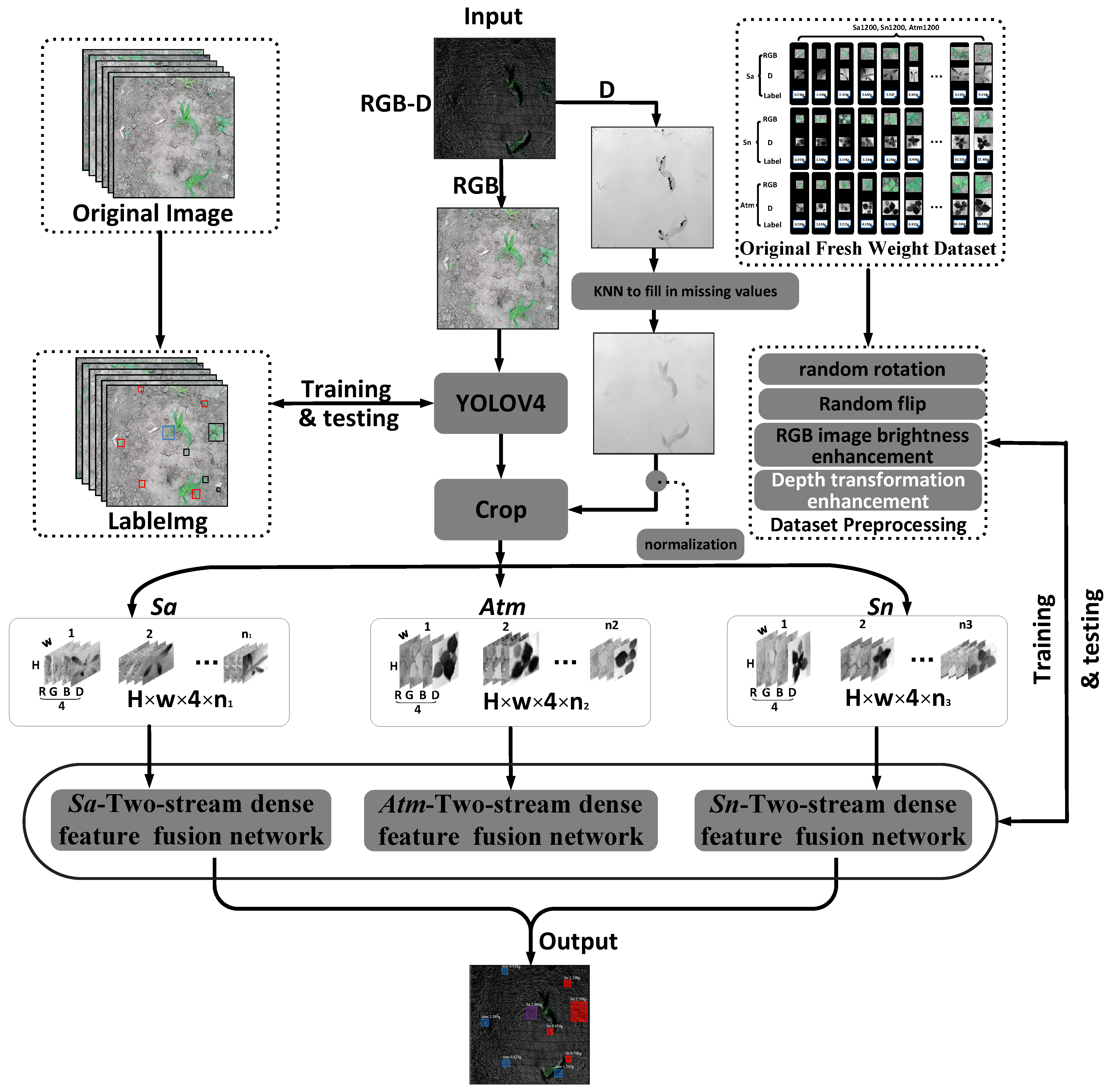
The main idea of the technical route proposed in this paper is to use YOLO-V4 to locate the target weeds and then send the obtained weed areas to the corresponding two-stream dense feature fusion network by category to predict their fresh weight on the ground. 
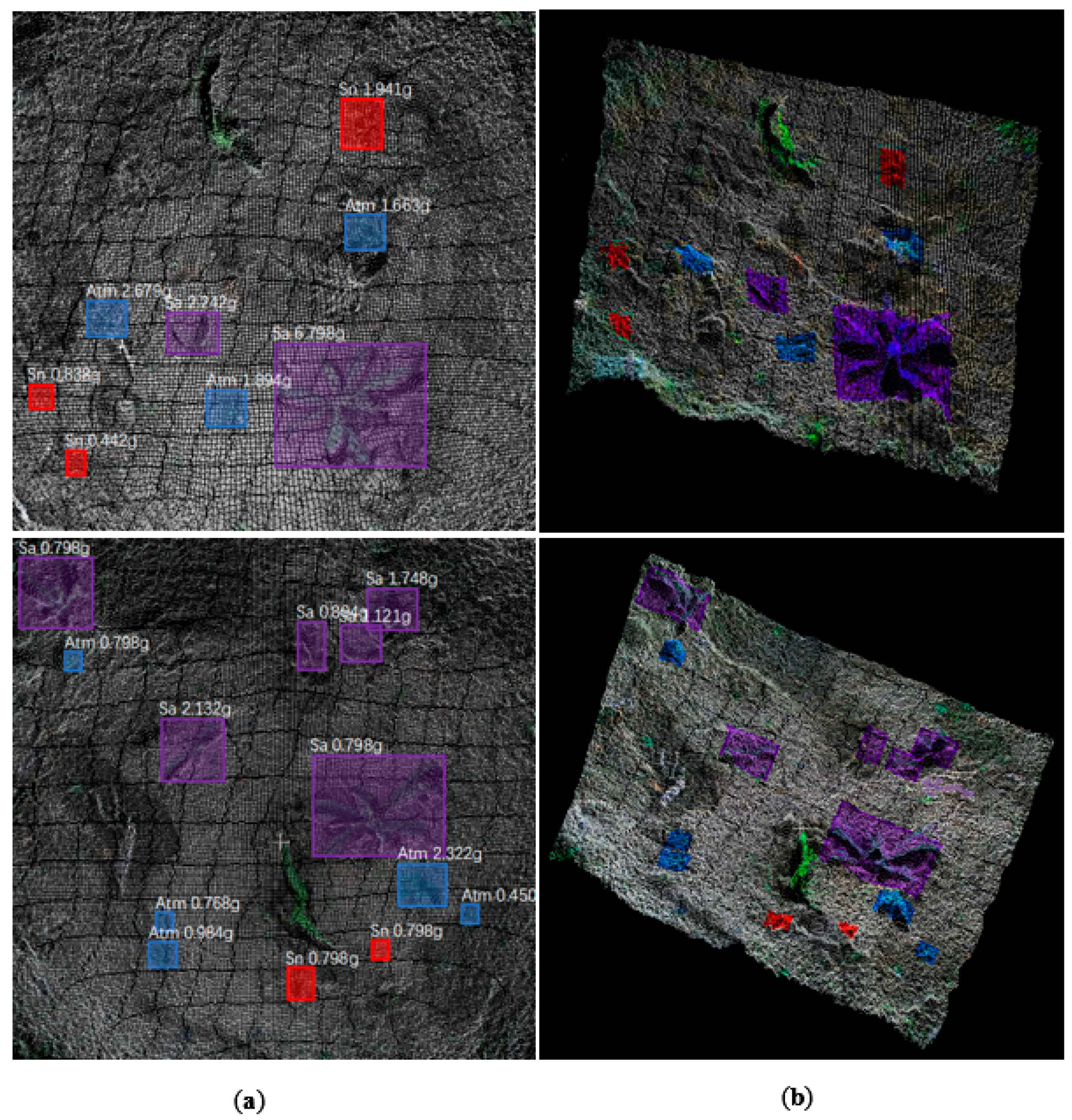
Figure 10 shows the results of the 3D visualization of the aboveground fresh weight detection of weeds (A visualization of the results of the two-stream dense feature fusion network on RGB images can be obtained in Figure A3 in the Appendix A). The mAP (IoU value of 0.5) of the model proposed in this paper is 75.34%, and the mIoU is 86.36%. When combining YOLO-V4 with the improved, fastest two-stream dense feature fusion network (AlexNet) model, the prediction speed is 17.8fps. The average relative error of the fresh weight of the weeds in the test set is approximately 4%. This model can provide visual technical support for precision variable-target platforms.

4.2. Comparison of YOLO-V4 with Other Target Detection Algorithms

To find the most suitable convolutional neural network for weed detection, this study compared the YOLO-V4 model with the SSD [59], YOLO-V5x [60], M2DNet [61], and Faster R-CNN [53] networks. Target detection networks can be divided into two main categories: one-stage target detection networks and two-stage target detection networks. The reason for selecting these four networks for comparison is that YOLO-V4, YOLO-V5x, SSD, and M2DNet are typical representative one-stage networks of different types, and their performance is relatively advanced. The Faster R-CNN network, a typical two-stage network, also exhibits advanced performance. Therefore, this article compares the performance advantages of these four types of networks with regard to the problem of weed detection. Table 2 shows the mAP scores (mAP is obtained at an IoU value of 0.5), mIoU values, and average detection times of the models.
In the above results, the mAP score of YOLO-V4 is 0.7534, which is higher than the scores of the other four models. This indicates that the combined recall performance and accuracy of YOLO-V4 is better than the other four models. the IoU value of YOLO-V4 is 0.8636, which is higher than the other four models. This indicates that YOLO-V4 is more accurate than the other four models in detecting bounding boxes. the average removal time of YOLO-V4 is 0.033 seconds, which is faster than the other three models. However, the detection speed of YOLO-V4 was slower compared to YOLO-V5x. In our test set1, the minimum pixel size that yolov4 can detect for Sonchus arvensis is 14 × 16, for Abutilon theophrasti Medicus 8 × 10, and for Solanum nigrum 7 × 11. YOLO-V4 is effective for small target weed detection.

4.3. Two-Stream Dense Feature Fusion Network (DenseNet201-Rgbd)

4.3.1. Comparison of Regression Network Results Embedded with the Dense-NiN Module

In describing the model, we mentioned that the Dense-NiN module can be embedded in a typical convolutional neural network. In the embedded VGG19 and AlexNet networks, we add a deep feature fusion layer after each pooling layer to receive the output of the Dense-NiN-Block module. In Inception-V3 and Resnet101, we add the Dense-NiN-Block module before the network convergence layer. The structure of DenseNet201 has been described above. The number of test set2 for each weed species is 300. This study integrates the Resnet101, VGG19, Inception-V3, AlexNet, and DenseNet201 networks of the Dense-NiN module for comparison to select the model with the best fit.
To compare the effects of weed species on the detection results, three weed species, Abutilon theophrasti Medicus, Solanum nigrum, and Sonchus arvensis, were used as training sets to train the convolutional neural network. At the same time, these three weed species were also merged into a single data set to train the model (abbreviated as all). Moreover, to compare RGB-D information and RGB information when using a convolutional network for fresh weight prediction, RGB and RGB-D were used as inputs for network training. The dual-stream dense fusion network architecture proposed in this paper used the RGB-D information for training. The RGB images were used directly with the default network structures of these five networks, and the output module of the original network needed only to be replaced with the output module proposed in this article to achieve a new regression. The RMSEs of the training models are shown in Figure 11, the R 2 values are shown in Table 3, and the average times (s) are shown in Table 4.
The above results show that, in all networks, the accuracy obtained using RGB-D data as the input is higher than that obtained using RGB as the input. This indicates that RBG-D stereo data can indeed provide more information for use in weed fresh weight evaluation. However, the speed usually decreases when RBG-D data are used. This is because the two-stream dense feature fusion network using RGB-D data introduces a denser convolution structure and increases the weight, which causes the speed to drop. In the regression test for the fresh weights of the three weed species, the RMSE values of the dual-stream dense fusion network (DenseNet201-rgbd) are 0.358 for Abutilon theophrasti Medicus, 0.416 for Solanum nigrum, and 0.424 for Sonchus arvensis (Notable among these is the closer detection of RGB-D and RGB for Sonchus arvensis compared to the other two weeds. We provide a specific analysis in session 4.3.3.). The value for all weeds is 0.568, which is higher than those of the other models. The RMSE values of the three aboveground fresh weight prediction models trained using this model are lower than the RMSE value of all weed models trained directly. Therefore, after applying YOLO-V4, a network that can be independently and successfully trained for each weed species can be adaptively selected, and its performance will be better than a trained network using all the weeds as the training set. The R 2 of the dual-stream dense fusion network (DenseNet201-rgbd) is also the highest, with a value of 0.9917 for Abutilon theophrasti Medicus, a value of 0.9921 for Solanum nigrum, and a value of 0.9885 for Sonchus arvensis. This network has a good fitting ability. Selecting the corresponding model according to the weed type output by YOLO-V4 does not affect the speed of the model. For example, there are 10 tensors in the output stream of YOLO-V4. Using a different model for each weed type or directly using all the trained weed models requires a calculation time of 10 tensors. The only difference is whether the network is selected according to the weed type. This kind of speed loss is almost negligible.
At the same time, the higher the accuracy of the detection model is, the slower the speed; if higher accuracy is desired, speed must be sacrificed to some extent. When the density of weeds in the environment is high, the accuracy of the model may be reduced, and a faster model can be selected. It is worth noting that the average detection speed of each model is 0.0359 for Solanum nigrum, 0.0378 for Sonchus arvensis, and 0.0390 for Abutilon theophrasti Medicus. We believe that this is due to the size of the weed test set2 image. We calculated the average image size of the three weeds in the test set2. The average size of Solanum nigrum is 104 × 108, the average size of Abutilon theophrasti Medicus is 166 × 175, and the average size of Sonchus arvensis is 150 × 158. The size of the weeds also affects the speed of the network. Therefore, reducing the image size uniformly during the training process of the two-stream dense feature fusion network and reducing the image size by the same proportion during the prediction process could help to improve the efficiency of the model.
On the other hand, we used a non-CNN technique to build a regression model with the canopy area of the weed as the independent variable and the aboveground fresh weight of the weed as the dependent variable. Using a polynomial fit method, Abutilon theophrasti Medicus obtained a minimum RMSE value of 3.632. Solanum nigrum obtained a minimum RMSE value of 3.246. Sonchus arvensis obtained a minimum RMSE value of 2.033. The experiments proved that that using the CNN technique is indeed better than using single factor regression. The method is more advantageous. In a real field environment, the ground is relatively uneven. For example, two identical weeds, one growing at a higher position and the other at a lower position, will have different RGB images even if the height of the camera is 800 mm. If above-ground fresh regression is performed using canopy pixel area, the weed growing in the higher position has a larger canopy pixel area and the weed growing in the lower position has a smaller canopy pixel area. This can lead to such errors, and depth data can help us to resolve such differences effectively.
In practical agricultural applications, the Chinese national standard (GB-T36007-2018) states that field weeding robots should operate at a speed of around 0.4 to 0.5 m per second. Our robots can operate effectively in real time with RGB-D while complying with the Chinese national standard. For us, faster speed is not as effective as more precise accuracy. In the future, robots will inevitably travel at higher speeds, so it is worth considering giving up a certain level of accuracy to use RGB images in the future. It is worth noting that YOLO-V5x is very fast and, although not as accurate as YOLO-V4, is smaller, making it easier for us to deploy to edge computing devices. We still need to evaluate the specific performance of YOLO-V4 and YOLO-V5x on edge computing devices such as the Jet-son AGX Xavier in future work.

4.3.2. The Impact of Different Data Enhancement Methods

To verify the influence of the four data augmentation methods described above in the training model, the control variable method was used to delete one data augmentation method at a time, and the RMSE values were obtained. The results are shown in Table 5.
According to the experimental results, random rotation and random flipping have limited impacts on the model, but excluding these two methods still reduces the detection accuracy. Removing random rotation increases the average RMSE of the model by 0.052, and removing random flipping increases the average RMSE of the model by up to 0.050. The device cover provides the function of a hood but still allows visible light to pass through. Brightness enhancement can help the model adapt to subtle changes in light. The results show that the result of removing the brightness enhancement transform is 0.115 higher than the RMSE value using the full enhancement method. The depth conversion enhancement function can help the model adapt to uneven ground. Depth enhancement greatly improves the performance of the detection model. If this method is excluded, the RMSE score of the detection model increases by 0.129. Therefore, the depth conversion enhancement method helps to improve the performance of the model.

4.3.3. The Two-Stream Dense Feature Fusion Network (DenseNet201) Is Affected by the Growth Period and Weed Species

To compare the responses of the RGB network and RGB-D network (DenseNet201-rgb and DenseNet201-rgbd) to weeds in different periods, we classified the three weed species by size from small to large according to the quality distribution of the test set. Every fifty adjacent weeds are considered as one stage, and six stages (A, B, C, D, E, and F) stages are considered in the analysis. Figure 12 shows the actual results for the three weed species.
Comparing the average RMSE value of the RGB data with the average RMSE value of the RGB-D data shows that in stages A and B, the RMSE value for Abutilon theophrasti Medicus increased by 0.113, that for Solanum nigrum decreased by 0.011, and that for Sonchus arvensis decreased by 0.162. The advantage of using RGB-D data is not obvious. In stages C and D, the RMSE for Abutilon theophrasti Medicus increased by 0.209, for Solanum nigrum weeds increased by 0.334, and for Sonchus arvensis increased by 0.111. The RMSE for Abutilon theophrasti Medicus and Solanum nigrum increased significantly, while the increase in the RMSE for Sonchus arvensis was relatively small. In stages E and F, the RMSE for Abutilon theophrasti Medicus weeds increased by 0.650, for Solanum nigrum increased by 0.628, and for Sonchus arvensis increased by 0.249. Compared with those in the first four stages, the RMSE increase for Abutilon theophrasti Medicus and Solanum nigrum was greater, while the increase for Sonchus arvensis was still relatively small. Overall, the RMSE values for Abutilon theophrasti Medicus and Solanum nigrum obtained using RGB images as input gradually increases, and the magnitude of the increase also increases. Although the RMSE value for Sonchus arvensis also exhibits an upward trend, the overall fluctuation is very small. Using RGB-D as the network input, the RMSE values for the predicted values of the weeds in the six stages all fluctuate slightly or even show a downward trend. The results show that in the later stages of weed growth, using RGB-D as the network input provides more stable and accurate results than using RGB as the network input.
In the early weed growth stages, the performances obtained using RGB and RGB-D as inputs are roughly the same. This shows that in the early stage, the regression model is more dependent on the overhead-view area of the plant for regression prediction. At this time, the weeds are very short, so the regression prediction results using RGB and RGB-D are nearly the same. In the subsequent growth stages, as the weeds gradually grow taller, the stems account for a certain percentage of the weight of the weeds, the height of the plants cannot be obtained from the RGB image, and the accuracy of predictions obtained using RGB images begins to decline. The scatter plots of the actual and predicted fresh weights of the weeds show that in the RGB prediction process, at the later stage of growth, the predicted fresh weight value is usually lower than the actual value. Due to a lack of height information, the predicted fresh weight value is too low. Therefore, the RGB-D model exhibits better robustness in the subsequent growth stages of weeds. However, in these six stages, the RMSE values of the results obtained using RGB-D and RGB images for Sonchus arvensis did not change substantially. Given the low height of these weed species, their aboveground fresh weight may depend more on their top-view area. In the early and late stages of growth, the difference between the RMSE values of the RGB and RGB-D predictions is not substantial, but RGB-D still provides a better fitting effect.

4.3.4. Model Analysis

(1)
Dense connections extract deep features
The Dense-NiN-Block module uses a dense connection structure. The dense structure allows access to all its previous feature maps (including transition layers). Our experiment investigates whether the trained network takes advantage of this opportunity. For each convolutional layer in a block, we calculate the average (absolute) weight assigned to the connection to layer s . Figure 13 shows the heat map of all four Dense-NiN-Block modules. The average absolute weight replaces the dependence of the convolutional layer on its previous layers. The red dot in position ( , s ) indicates that the layer uses the feature map of the previously generated s layer on average.
The figure shows that all layers spread their weights over many inputs within the same block. The feature information from the weed depth data obtained in the early stages of the network is actually used by the deeper convolution filters within the same dense block. The weights of the transition layers also spread their weight across all layers within the preceding dense block, indicating information flow from the first to the last layers of the Dense module through few indirections. Therefore, the NiN module in this study effectively uses the Dense connection method to enhance the use of weed depth information.
(2)
Model visualization analysis
To explore which information made the greatest contribution to fresh weight prediction as well as the specific impact of depth data, we use Grad-CAM to visualize the network and compare the differences between the RGB-D network and RGB network models (DenseNet201-rgb and DenseNet201-rgbd). Figure 14 shows the visualization results. Areas with a high thermal value represent the greatest utilization of the feature map of the pixel area.
As shown in Figure 14, these two networks have learned the channel pixels within the weed area in order to make fresh weight predictions. In the Grad-CAM map output by two-stream dense feature fusion network, the heat value near the middle of the weed area is higher than that at the edges of the weed area. We believe that this phenomenon occurs because the central area of the plant, as the main growth point of the stem, has obviously different height characteristics than the other plant parts. This leads to a large difference between the depth data in this part and in other parts, and this difference can improve the weed fresh weight prediction function of the model; in contrast, the RGB network does not have such advantages. In addition, our model not only considers to the information within the weed outline but also considers the periphery of the weed area (shown in the red circles in the figure). In the actual environment, the ground cannot be flat. Although the camera is set at a distance of 800 mm from the ground, it cannot actually be stabilized at that distance. Due to the unevenness of the ground, the camera position fluctuates around 800 mm above the ground. This results in some weeds being detected in low-lying positions, while some weeds are perceived as being relatively tall. For example, for two weeds of the same quality, the RGB image of the taller weed is larger due to the difference in geographic location, which makes the RGB network prediction value higher. From the perspective of depth data, the depth data value of shorter weeds is higher, and the depth data value of taller weeds is lower. The depth information of the weed outline area does not directly reflect this difference, but the depth data outside the weed outline directly reflects the distance between the camera and the ground. The figure above shows that distance information is also regarded as an important difference feature by the network. At the same time, the information inside and outside the weed outline constitutes the height information for the weed. The high thermal response outside the weed outline area indicates that the network has learned this indirect relationship. Therefore, the value of information outside the range of weed outlines is also used effectively. The RGB network cannot resolve the imaging difference caused by the fluctuation of the distance between the camera and the ground. On the other hand, we explored the results of using only data within the RGB-D weed contour lines. The RMSE results obtained using the network proposed in this paper showed 0.648 for Abutilon theophrasti Medicus, 0.824 for Solanum nigrum, and 0.481 for Sonchus arvensis, all lower than the method used in this paper and more evidence of the importance of ground-to-camera distance information in depth images (areas beyond the weed contour lines). distance information in the depth images (the area beyond the weed contour line).

4.4. The Relationship between IOU and Fresh Weight Prediction

In this study, manual trimming was used to create the data set when training the network. However, when using the two-stream dense feature fusion network model, the output of the YOLO-V4 model was actually accepted. There are certain differences between the two. The specific response to this difference is reflected in the IoU values, so this article compares the RMSE under different IoU values. To specifically reflect the impact of manual trimming and the YOLO-V4 output data on the accuracy of fresh weight prediction. The comparison was performed to reflect the difference in accuracy. The results are shown in Table 6.
The results above show that the IOU value will have a slight impact on the prediction result. When the IOU value is greater than 50%, the RMSE values for the three weed species using the YOLO-V4 network result as the input prediction value and those using the manual trimming result as the input prediction value are 0.065, 0.034, and 0.060, respectively, and show little difference. However, as the IOU value decreases, the RMSE value gradually increases, and the network prediction accuracy decreases. These results demonstrate that the IOU value affects the accuracy of the two-stream dense feature fusion network. In this article, the IOU threshold for YOLO-V4 is selected as 0.5. Appropriately increasing the IOU threshold can make the network fitting effect more accurate.

4.5. Predictive Effects for Shaded Weeds

In the early stages of corn cultivation, weeds are small and rarely cover each other. During this period, individual weeds are easy to distinguish. However, as the weeds continue to grow, the degree of overlap between them increases, and it becomes more difficult to distinguish them. YOLO-V4 can identify weeds that have a certain degree of overlap, but misidentifications can still occur. Instances of misrecognition can be classified into three situations:
  • When two weeds cover each other, the network divides them into uniform individuals, as shown by the red bounding box.
  • When two weeds cover each other, the network identifies only part of the weed but not the whole weed, as shown by the purple bounding boxes.
  • When two weeds shade each other, the weed cannot be detected, as shown by the black arrow in (a).
Figure 15a shows a situation in which, because of mutual covering, two weeds are identified as one. Sonchus arvensis is a weed species that relies heavily on its stems to reproduce multiple aboveground parts on the same root that usually overlap considerably and are close together. Therefore, it is easy for mistakes to occur during detection. Figure 15b,c show the occlusion of Solanum nigrum and Abutilon theophrasti Medicus. Unlike Sonchus arvensis, Solanum nigrum and Abutilon theophrasti Medicus have distinct individual characteristics, do not share the same root system, and are usually farther apart. Even if there is occlusion, partial recognition can be achieved, but the abovementioned problems still exist. These problems will affect the accuracy of the subsequent aboveground fresh weight prediction. The first type of error will result in the calculation of the aboveground fresh weight of the provided weed patch data, and the second type of error will cause the prediction value to be too small. However, the purpose of this article is to provide visual support for precise adjustments to herbicide application. Except for the small number of errors of the third type, the detection errors observed in this study would have little effect on variable herbicide application. Therefore, the research in this article still has practical significance.

5. Conclusions

In this study, we propose a new concept for the real-time detection of the aboveground fresh weight of weeds to provide visual support for precision variable herbicide spraying. At the same time, a new model that can detect weeds and predict their fresh weight in real time in the field is developed. The algorithm combines deep learning technology with 3D data. This paper proposes a strategy of using the YOLO-V4 target detection network to obtain the regional weed area and then send the RGB-D data for the weed area into a dual-stream dense feature fusion network regression model to perform a regression on the fresh weight data so that the fresh weight of weeds can be predicted. The error of the model is approximately 4%, and the fastest detection speed is 17.8 fps. To construct a data set for training these two networks, a data collection method that establishes a labelling method is proposed. This method can quickly establish the relationship between the weed RGB-D data and the fresh weight data while avoiding interference with the actual operating environment. When predicting the fresh weight of weeds taller than a certain height, more accurate results are achieved using RGB-D information as the input for the model. The visualization results show that the use of a two-stream dense feature fusion network can better address the imaging differences caused by the uneven land surface and make the predictions more accurate.
In this paper we have only done a preliminary exploration of fresh weight models for three weeds, the richness of weed species is still lacking, and the next step of the workshop is to enrich our weed types. Future work will focus on determining the type and fresh weight of weeds in order to determine the appropriate amount of herbicides to apply in real time, optimizing weeding strategies to reduce the use of herbicides, and applying the model to a variable herbicide-application robot. The approaches used to develop this model can also be extended to the prediction of the fresh weight of crop plants, which could provide support for crop breeding and genetic improvement as well as soil health.

Author Contributions

L.Q. and H.L. (Hengda Li) prepared the manuscript; H.L. (Hailong Li), W.J. and Z.L. collected the data; H.L. (Hengda Li) developed the codes; L.Q. and L.C. supervised the project. All authors have read and agreed to the published version of the manuscript.

Funding

The authors gratefully appreciate the National Natural Science Foundation of China (52075092) and the Provincial Postdoctoral Landing Project (LBH-Q19007).

Institutional Review Board Statement

Not applicable.

Informed Consent Statement

Not applicable.

Data Availability Statement

Given that the data used in this study were self-collected, the dataset is being further improved. Thus, the dataset is unavailable at present.

Acknowledgments

The authors gratefully appreciate the National Natural Science Foundation of China (52075092) and the Provincial Postdoctoral Landing Project (LBH-Q19007).

Conflicts of Interest

The authors declare no conflict of interest.

Appendix A

Figure A1. Enlarged supplement to Figure 1D.
Remotesensing 13 02288 g0a1
Figure A2. Training set2 and test set2 distributions.
Remotesensing 13 02288 g0a2
Figure A3. Visualization of the results of two-stream dense feature fusion network on RGB images. Notes: Labels in order of species, confidence, aboveground fresh weight.
Remotesensing 13 02288 g0a3

References

  1. Zimdahl, R.L. Chapter 13—Introduction to Chemical Weed Control. In Fundamentals of Weed Science, 5th ed.; Academic Press: Waltham, MA, USA, 2018; pp. 391–416. [Google Scholar]
  2. Gil, Y.; Sinfort, C. Emission of pesticides to the air during sprayer application: A bibliographic review. Atmos. Environ. 2005, 39, 5183–5193. [Google Scholar] [CrossRef]
  3. Heap, I.; Duke, S.O. Overview of glyphosate-resistant weeds worldwide. Pest Manag. Sci. 2018, 74, 1040–1049. [Google Scholar] [CrossRef]
  4. Hall, D.; Dayoub, F.; Perez, T.; McCool, C. A rapidly deployable classification system using visual data for the application of precision weed management. Comput. Electron. Agric. 2018, 148, 107–120. [Google Scholar] [CrossRef] [Green Version]
  5. Partel, V.; Kakarla, C.; Ampatzidis, Y. Development and evaluation of a low-cost and smart technology for precision weed management utilizing artificial intelligence. Comput. Electron. Agric. 2019, 157, 339–350. [Google Scholar] [CrossRef]
  6. Cobb, A.H.; Reade, J.P. Herbicides and Plant Physiology; John Wiley & Sons: Hoboken, NJ, USA, 2011. [Google Scholar]
  7. Walker, S.; Boucher, L.; Cook, T.; Davidson, B.; McLean, A.; Widderick, M. Weed age affects chemical control of Conyza bonariensis in fallows. Crop Prot. 2012, 38, 15–20. [Google Scholar] [CrossRef]
  8. Kieloch, R.; Domaradzki, K. The role of the growth stage of weeds in their response to reduced herbicide doses. Acta Agrobot. 2011, 64, 259–266. [Google Scholar] [CrossRef]
  9. Dayan, F.E.; Barker, A.; Bough, R.; Ortiz, M.; Takano, H.; Duke, S.O.; Moo-Young, M. 4.04—Herbicide Mechanisms of Action and Resistance. In Comprehensive Biotechnology, 3rd ed.; Pergamon: Oxford, UK, 2019; pp. 36–48. [Google Scholar]
  10. Sterling, T.M. Mechanisms of Herbicide Absorption across Plant Membranes and Accumulation in Plant Cells. Weed Sci. 1994, 42, 263–276. [Google Scholar] [CrossRef]
  11. Holt, J.S.; Levin, S.A. Herbicides. In Encyclopedia of Biodiversity, 2nd ed.; Academic Press: Waltham, MA, USA, 2013; pp. 87–95. [Google Scholar]
  12. Huang, W.; Ratkowsky, D.A.; Hui, C.; Wang, P.; Su, J.; Shi, P. Leaf Fresh Weight Versus Dry Weight: Which is Better for Describing the Scaling Relationship between Leaf Biomass and Leaf Area for Broad-Leaved Plants? Forests 2019, 10, 256. [Google Scholar] [CrossRef] [Green Version]
  13. Bredmose, N.; Hansen, J. Topophysis affects the Potential of Axillary Bud Growth, Fresh Biomass Accumulation and Specific Fresh Weight in Single-stem Roses (Rosa hybridaL.). Ann. Bot. 1996, 78, 215–222. [Google Scholar] [CrossRef] [Green Version]
  14. Jiang, J.-S.; Kim, H.-J.; Cho, W.-J. On-the-go image processing system for spatial mapping of lettuce fresh weight in plant factory. IFAC-PapersOnLine 2018, 51, 130–134. [Google Scholar] [CrossRef]
  15. Arzani, K.; Lawes, S.; Wood, D. Estimation of ‘sundrop’ apricot fruit volume and fresh weight from fruit diameter. Acta Hortic. 1999, 321–326. [Google Scholar] [CrossRef]
  16. Reyes-Yanes, A.; Martinez, P.; Ahmad, R. Real-time growth rate and fresh weight estimation for little gem romaine lettuce in aquaponic grow beds. Comput. Electron. Agric. 2020, 179, 105827. [Google Scholar] [CrossRef]
  17. Mortensen, A.K.; Bender, A.; Whelan, B.; Barbour, M.M.; Sukkarieh, S.; Karstoft, H.; Gislum, R. Segmentation of lettuce in coloured 3D point clouds for fresh weight estimation. Comput. Electron. Agric. 2018, 154, 373–381. [Google Scholar] [CrossRef]
  18. Lee, S.; Kim, K.S. Estimation of fresh weight for chinese cabbage using the Kinect sensor. Korean J. Agric. For. Meteorol. 2018, 20, 205–213. [Google Scholar]
  19. Wang, A.; Zhang, W.; Wei, X. A review on weed detection using ground-based machine vision and image processing techniques. Comput. Electron. Agric. 2019, 158, 226–240. [Google Scholar] [CrossRef]
  20. Raja, R.; Nguyen, T.T.; Slaughter, D.C.; Fennimore, S.A. Real-time weed-crop classification and localisation technique for robotic weed control in lettuce. Biosyst. Eng. 2020, 192, 257–274. [Google Scholar] [CrossRef]
  21. Mottley, J.; Keen, B. Indirect assessment of callus fresh weight by non-destructive methods. Plant Cell Rep. 1987, 6, 389–392. [Google Scholar] [CrossRef]
  22. Sandmann, M.; Graefe, J.; Feller, C. Optical methods for the non-destructive estimation of leaf area index in kohlrabi and lettuce. Sci. Hortic. 2013, 156, 113–120. [Google Scholar] [CrossRef]
  23. Jung, D.-H.; Hyun, P.S.; Xiongzhe, H.; Hakjin, K. Image Processing Methods for Measurement of Lettuce Fresh Weight. J. Biosyst. Eng. 2015, 40, 89–93. [Google Scholar] [CrossRef] [Green Version]
  24. Feyaerts, F.; van Gool, L. Multi-spectral vision system for weed detection. Pattern Recognit. Lett. 2001, 22, 667–674. [Google Scholar] [CrossRef]
  25. Shirzadifar, A.; Bajwa, S.; Mireei, S.A.; Howatt, K.; Nowatzki, J. Weed species discrimination based on SIMCA analysis of plant canopy spectral data. Biosyst. Eng. 2018, 171, 143–154. [Google Scholar] [CrossRef]
  26. Pantazi, X.-E.; Moshou, D.; Bravo, C. Active learning system for weed species recognition based on hyperspectral sensing. Biosyst. Eng. 2016, 146, 193–202. [Google Scholar] [CrossRef]
  27. Zhang, Y.; Slaughter, D.C. Hyperspectral species mapping for automatic weed control in tomato under thermal environmental stress. Comput. Electron. Agric. 2011, 77, 95–104. [Google Scholar] [CrossRef]
  28. Hamuda, E.; Mc Ginley, B.; Glavin, M.; Jones, E. Automatic crop detection under field conditions using the HSV colour space and morphological operations. Comput. Electron. Agric. 2017, 133, 97–107. [Google Scholar] [CrossRef]
  29. Tang, J.-L.; Chen, X.-Q.; Miao, R.-H.; Wang, D. Weed detection using image processing under different illumination for site-specific areas spraying. Comput. Electron. Agric. 2016, 122, 103–111. [Google Scholar] [CrossRef]
  30. Tannouche, A.; Sbai, K.; Rahmoune, M.; Zoubir, A.; Agounoune, R.; Saadani, R.; Rahmani, A. A Fast and Efficient Shape Descriptor for an Advanced Weed Type Classification Approach. Int. J. Electr. Comput. Eng. 2016, 6, 1168. [Google Scholar]
  31. Pérez, A.J.; López, F.; Benlloch, J.V.; Christensen, S. Colour and shape analysis techniques for weed detection in cereal fields. Comput. Electron. Agric. 2000, 25, 197–212. [Google Scholar] [CrossRef]
  32. Lin, F.; Zhang, D.; Huang, Y.; Wang, X.; Chen, X. Detection of Corn and Weed Species by the Combination of Spectral, Shape and Textural Features. Sustainability 2017, 9, 1335. [Google Scholar] [CrossRef] [Green Version]
  33. Zheng, Y.; Zhu, Q.; Huang, M.; Guo, Y.; Qin, J. Maize and weed classification using color indices with support vector data description in outdoor fields. Comput. Electron. Agric. 2017, 141, 215–222. [Google Scholar] [CrossRef]
  34. Swain, K.C.; Nørremark, M.; Jørgensen, R.N.; Midtiby, H.S.; Green, O. Weed identification using an automated active shape matching (AASM) technique. Biosyst. Eng. 2011, 110, 450–457. [Google Scholar] [CrossRef]
  35. Kazmi, W.; Garcia-Ruiz, F.; Nielsen, J.; Rasmussen, J.; Andersen, H.J. Exploiting affine invariant regions and leaf edge shapes for weed detection. Comput. Electron. Agric. 2015, 118, 290–299. [Google Scholar] [CrossRef]
  36. Bakhshipour, A.; Jafari, A. Evaluation of support vector machine and artificial neural networks in weed detection using shape features. Comput. Electron. Agric. 2018, 145, 153–160. [Google Scholar] [CrossRef]
  37. Tian, Y.; Yang, G.; Wang, Z.; Wang, H.; Li, E.; Liang, Z. Apple detection during different growth stages in orchards using the improved YOLO-V3 model. Comput. Electron. Agric. 2019, 157, 417–426. [Google Scholar] [CrossRef]
  38. Quan, L.; Feng, H.; Li, Y.; Wang, Q.; Zhang, C.; Liu, J.; Yuan, Z. Maize seedling detection under different growth stages and complex field environments based on an improved Faster R-CNN. Biosyst. Eng. 2019, 184, 1–23. [Google Scholar] [CrossRef]
  39. Hu, K.; Coleman, G.; Zeng, S.; Wang, Z.Y.; Walsh, M. Graph weeds net: A graph-based deep learning method for weed recognition. Comput. Electron. Agric. 2020, 174, 9. [Google Scholar] [CrossRef]
  40. Dos Santos Ferreira, A.; Matte Freitas, D.; Gonçalves da Silva, G.; Pistori, H.; Theophilo Folhes, M. Weed detection in soybean crops using ConvNets. Comput. Electron. Agric. 2017, 143, 314–324. [Google Scholar] [CrossRef]
  41. Hasan, A.S.M.M.; Sohel, F.; Diepeveen, D.; Laga, H.; Jones, M.G.K. A survey of deep learning techniques for weed detection from images. Comput. Electron. Agric. 2021, 184, 106067. [Google Scholar] [CrossRef]
  42. Yu, J.; Sharpe, S.M.; Schumann, A.W.; Boyd, N.S. Deep learning for image-based weed detection in turfgrass. Eur. J. Agron. 2019, 104, 78–84. [Google Scholar] [CrossRef]
  43. Peteinatos, G.G.; Reichel, P.; Karouta, J.; Andújar, D.; Gerhards, R. Weed Identification in Maize, Sunflower, and Potatoes with the Aid of Convolutional Neural Networks. Remote Sens. 2020, 12, 4185. [Google Scholar] [CrossRef]
  44. Jiang, H.; Zhang, C.; Qiao, Y.; Zhang, Z.; Zhang, W.; Song, C. CNN feature based graph convolutional network for weed and crop recognition in smart farming. Comput. Electron. Agric. 2020, 174, 105450. [Google Scholar] [CrossRef]
  45. Zhou, J.; Fu, X.; Zhou, S.; Zhou, J.; Ye, H.; Nguyen, H.T. Automated segmentation of soybean plants from 3D point cloud using machine learning. Comput. Electron. Agric. 2019, 162, 143–153. [Google Scholar] [CrossRef]
  46. Li, J.; Tang, L. Developing a low-cost 3D plant morphological traits characterization system. Comput. Electron. Agric. 2017, 143, 1–13. [Google Scholar] [CrossRef] [Green Version]
  47. Chaivivatrakul, S.; Tang, L.; Dailey, M.N.; Nakarmi, A.D. Automatic morphological trait characterization for corn plants via 3D holographic reconstruction. Comput. Electron. Agric. 2014, 109, 109–123. [Google Scholar] [CrossRef] [Green Version]
  48. Li, Z.; Guo, R.; Li, M.; Chen, Y.; Li, G. A review of computer vision technologies for plant phenotyping. Comput. Electron. Agric. 2020, 176, 105672. [Google Scholar] [CrossRef]
  49. Sapkota, B.; Singh, V.; Neely, C.; Rajan, N.; Bagavathiannan, M. Detection of Italian Ryegrass in Wheat and Prediction of Competitive Interactions Using Remote-Sensing and Machine-Learning Techniques. Remote Sens. 2020, 12, 2977. [Google Scholar] [CrossRef]
  50. Krizhevsky, A.; Sutskever, I.; Hinton, G.E. ImageNet Classification with Deep Convolutional Neural Networks. Commun. Acm. 2017, 60, 84–90. [Google Scholar] [CrossRef]
  51. Schmidhuber, J. Deep learning in neural networks: An overview. Neural Netw. 2015, 61, 85–117. [Google Scholar] [CrossRef] [PubMed] [Green Version]
  52. Bawden, O.; Kulk, J.; Russell, R.; McCool, C.; English, A.; Dayoub, F.; Lehnert, C.; Perez, T. Robot for weed species plant-specific management. J. Field Robot. 2017, 34, 1179–1199. [Google Scholar] [CrossRef]
  53. Ren, S.; He, K.; Girshick, R.; Sun, J. Faster R-CNN: Towards Real-Time Object Detection with Region Proposal Networks. arXiv 2015, arXiv:1506.01497. [Google Scholar] [CrossRef] [Green Version]
  54. Bochkovskiy, A.; Wang, C.-Y.; Liao, H.-Y.M. YOLOv4: Optimal Speed and Accuracy of Object Detection. arXiv 2020, arXiv:2004.10934. [Google Scholar]
  55. Redmon, J.; Farhadi, A. YOLOv3: An Incremental Improvement. arXiv 2018, arXiv:1804.02767. [Google Scholar]
  56. Tzutalin, D. Labelimg. 2018. Available online: https://github.com/tzutalin/labelImg (accessed on 10 June 2021).
  57. Bengio, Y.; Courville, A.; Vincent, P. Representation Learning: A Review and New Perspectives. IEEE Trans. Softw. Eng. 2013, 35, 1798–1828. [Google Scholar] [CrossRef]
  58. Lin, M.; Chen, Q.; Yan, S. Network In Network. arXiv 2013, arXiv:1312.4400. [Google Scholar]
  59. Liu, W.; Anguelov, D.; Erhan, D.; Szegedy, C.; Reed, S.; Fu, C.-Y.; Berg, A.C. SSD: Single Shot MultiBox Detector. arXiv 2015, arXiv:1512.02325. [Google Scholar]
  60. Ultralytics/yolov5: V4.0 nn.SiLU() Activations, Weights & Biases Logging, PyTorch Hub Integration. 2021. Available online: https://explore.openaire.eu/search/software?softwareId=r37b0ad08687::14e263719066a7bd19d7916893c6f127 (accessed on 10 June 2021).
  61. Zhao, Q.; Sheng, T.; Wang, Y.; Tang, Z.; Chen, Y.; Cai, L.; Ling, H. M2Det: A Single-Shot Object Detector based on Multi-Level Feature Pyramid Network. arXiv 2018, arXiv:1811.04533. [Google Scholar] [CrossRef]
Figure 1. Data collection process. (AD) correspond to each of the four steps of the collection method in this section. The solid line in the figure represents the field of view of the camera, and the dotted line represents the range of the setting line. The different colored circles represent the respective categories of weeds. The weeds marked with a red cross in the picture represent no recording and collection. In (D), weeds are sorted from left to right according to leaf age and growth size. A detailed enlarged image is shown in Figure A1 in the Appendix A to this paper.
Remotesensing 13 02288 g001
Figure 2. Technical route. The content in the dashed box in the figure represents the training and testing process of the model described in this article. The other modules represent the flow chart to realize the functions of this research. Among them, Abutilon theophrasti Medicus is abbreviated as Atm, Sonchus arvensis is abbreviated as Sa, and Solanum nigrum is abbreviated as Sn.
Remotesensing 13 02288 g002
Figure 3. The result of using KNN to repair images with deep missing values. The first line of the image shows the gradual increase of the missing depth value from left to right. The bottom of each picture in the first row corresponds to the result after using KNN to repair.
Remotesensing 13 02288 g003
Figure 4. Training loss curve of the YOLO-V4 weed detection model.
Remotesensing 13 02288 g004
Figure 5. Two-stream dense feature fusion network (DenseNet201). The module color in the figure corresponds to the color comment block in the lower right corner. Batch Normalization is abbreviated as BN, and Rectified Linear Unit is abbreviated as Relu.
Remotesensing 13 02288 g005
Figure 6. Dense-Block structure.
Remotesensing 13 02288 g006
Figure 7. Dense-NiN-Block structure sends the feature extraction map to the process representation of Dense-Block structure. In this picture, the contents of the boxes indicates the Dense-NiN-Block structure. Xn indicates the feature map output by each convolutional layer in the RGB stream. Dn indicates the feature map output by each layer of convolution in the depth stream. Hn represents the feature map fusion layer.
Remotesensing 13 02288 g007
Figure 8. YOLO-V4 output data stream. In this figure, H × W × 4 × n, H, W indicate the size of the cropped image of each weed detected, 4 represents the number of RGB-D channels, n represents the number of each weed in the picture, each type of weed. The number of grass is different, n1, n2, and n3 are used to indicate this.
Remotesensing 13 02288 g008
Figure 9. Schematic diagram of depth transformation enhancement. The parameters in the figure are consistent with Equations (5) and (6). (a) shows the effect of the picture in the high and low states. (b) the data in blue in the upper half represent the original data and the data in red in the lower half represent the enhanced data. The change in size of the RGB image can clearly be seen in the change. In value of the D matrix, the larger the value of the D matrix the darker the color.
Remotesensing 13 02288 g009
Figure 10. Weed detection and fresh weight prediction results. (a) is an overhead view of the weed detection results, and (b) is a side view. Among them, Abutilon theophrasti Medicus is abbreviated as Atm, Sonchus arvensis is abbreviated as Sa, and Solanum nigrum is abbreviated as Sn.
Remotesensing 13 02288 g010
Figure 11. Comparison of weed fresh weight predictions with RMSE values.
Remotesensing 13 02288 g011
Figure 12. Fitting results for the three weed species. A, B, C, D, E, F represent the six stages of fresh weight on each weed from small to large, and each stage contains 50 weeds. In the scatter chart, True represents the true value of the weeds, the yellow point represents the predicted value using DenseNet201-rgb, and the green point represents the predicted value using DenseNet201-rgbd. In the line chart, the blue point represents the use at this stage The average RMSE value predicted by DenseNet201-rgb. The red dot indicates the average RMSE value predicted by DenseNet201-rgbd at this stage.
Remotesensing 13 02288 g012
Figure 13. Visualization effect charts. The average absolute filter weights of the convolutional layers in a trained DenseNet201. The color of the pixel at ( s , ) encodes the average L 1 norm (normalized by the number of input feature maps) of the weights connecting convolutional layer s to within a dense block. The three columns highlighted by black rectangles correspond to two transition layers and the classification layer. The first row encodes the weights connected to the input layer of the dense block.
Remotesensing 13 02288 g013
Figure 14. Grad-CAM comparison. This figure shows the visualization results. The red circle in the figure shows the ground area.
Remotesensing 13 02288 g014
Figure 15. (ac) show the different conditions in which weeds are shaded. The green boxes represent correctly identified weeds. The red boxes represent the recognition of several weeds as one weed. The purple boxes indicate that the network identified only part of the weeds. The black arrow indicates a weed that was not detected due to occlusion.
Remotesensing 13 02288 g015
Table 1. Summary of the dataset.
DateTotal ImagesSnAtmSaWeather
15 May 20202106120116128Cloud
16 May 20202453134133137Cloud
18 May 20201846120115120Cloud
19 May 20202152124108124Cloud
20 May 20202386126122122Cloud
21 May 20201919118115106Cloud
22 May 20201052759495Cloud
23 May 20201776968686Cloud
27 May 2020793587748Clear
28 May 2020737484966Clear
29 May 20201816969685Clear
30 May 20201238858983Clear
Total20274120012001200\
Notes: Among them, Abutilon theophrasti Medicus is abbreviated as Atm, Sonchus arvensis is abbreviated as Sa, and Solanum nigrum is abbreviated as Sn.
Table 2. Network comparison results.
ModelM2DNetSSDFaster R-CNNYOLO-V5xYOLO-V4
mAP (%)69.4164.3671.2373.2375.34
mIoU (%)84.2482.6386.3385.6286.36
Average time (s)0.1260.1920.2380.0160.033
Table 3. Network R 2 results.
ModelAtm R 2 Sn   R 2 Sa   R 2 All     R 2
Alexnet-rgb0.85150.83270.83220.7541
Alexnet-rgbd0.86220.87420.84140.7836
Vgg19-rgb0.87210.88560.86530.7621
Vgg19-rgbd0.88260.89430.86990.7834
Xception-rgb0.91320.90180.90150.7562
Xception-rgbd0.91440.91260.91130.8314
Resnet101-rgb0.93140.91420.91540.8734
Resnet101-rgbd0.95260.95340.93360.8852
DenseNet201-rgb0.96740.97510.94650.9154
DenseNet201-rgbd0.99170.99210.98850.9433
Table 4. Network average time results.
Average Time (s)
ModelAtmSnSaAll
Alexnet-rgb0.01380.01130.01270.0122
Alexnet-rgbd0.02460.02250.02330.0235
Vgg19-rgb0.01330.01250.01960.0158
Vgg19-rgbd0.03260.02470.02960.0311
Xception-rgb0.02670.02260.02370.0259
Xception-rgbd0.04420.04260.03940.0463
Resnet101-rgb0.03480.03130.03330.0329
Resnet101-rgbd0.06220.06360.06240.0618
DenseNet201-rgb0.04960.04540.04410.0456
DenseNet201-rgbd0.08790.08210.08950.0846
Average0.03900.03590.03780.0380
Table 5. Data enhancement control variable comparison.
Data Augmentation MethodATM RMSESn RMSESa RMSEAverage
Dataset after augmentation0.3580.4160.4240.400
Random rotation0.3860.4790.4910.452
Random flip0.4010.4960.4530.450
RGB brightness enhanced by 10% 0.4520.5310.5620.515
Depth transformation enhancement0.5040.5660.5160.529
Table 6. Impact of mIOU on RMSE.
mIOUAtm RMSESn RMSESa RMSE
90~100%0.0260.0140.023
80~90%0.0380.0210.036
70~80%0.0610.0160.057
60~70%0.0870.0540.089
50~60%0.1120.0670.093
Average0.0650.0340.060
Publisher’s Note: MDPI stays neutral with regard to jurisdictional claims in published maps and institutional affiliations.

