Abstract
Remote sensing (RS)-derived vegetation indices (VIs) with medium and high spatial resolution have emerged as a promising dataset for fine-scale ecosystem modeling and agricultural monitoring at local or global scales. Before they can be used as reliable inputs for other research, conducting in situ measurements for validation is very critical. However, the spatial heterogeneity due to the diversity of land cover and its spatial organization in the landscape increases the uncertainty of validation, so design of optimal sampling is an important basis for the reliability of the validation. In this paper, we propose an integrative stratified sampling strategy (INTEG-STRAT) based on normalized difference vegetation index (NDVI) data as prior knowledge. The basic idea is to realize a sampling optimization by determining the optimal combination of the spatial sampling method (e.g., simple random sampling (SRS), spatial system sampling (SYS), stratified sampling, generalized random tessellation stratified (GRTS), balanced acceptance sampling (BAS)) and spatial stratification scheme with an objective rule. The objective rule in this paper is to minimize the root mean square error (RMSE) of 10-fold cross validation between estimated values (sample are not included) and the corresponding values on prior knowledge. Relative precision, correlation coefficient, and RMSE are used to compare the effectiveness of the proposed sampling strategy with each sampling method without considering sampling optimization. After comparing, we find that the INTEG-STRAT requires fewer samples to become stable and has higher accuracy. At site 1, when the correlation coefficient between NDVI image and the simulated NDVI surface reached 80%, INTEG-STRAT needed only 70 sampling points while other methods require more sampling points. At the same time, INTEG-STRAT strategy has a smaller RMSE between the estimated values and the corresponding values on prior knowledge image. In general, INTEG-STRAT is an effective method in the selection of representative samples to support the validation of vegetation indices products with medium and high spatial resolution.
1. Introduction
Vegetation can have a significant effect on hydrological fluxes due to variations in the physical characteristics of the land surface, soil, and vegetation [1,2]. The spectral vegetation indices (VIs), based on remotely sensed reflectance in the near-infrared and visible bands, are deemed as the fundamental and most widely used indicators for many regional and global ecological and environmental applications [3,4]. At present, Moderate Resolution Imaging Spectroradiometer (MODIS) VIs are still a good choice for regional or global research due to their long time series (from 2000 to present) and spatial and temporal consistency. However, due to the relatively coarse spatial resolution from 250 to 1000 m, it can be difficult to detect vegetation characteristics in heterogeneous landscapes on a local scale. In recent years with the improvement of satellite technology, satellite temporal and spatial resolution has increased greatly, which may provide more appropriate spatial and temporal resolutions to describe such heterogeneous regions. For example, revisit frequency for Gaofen-1 (GF-1) wide-field-of-view (WFV) camera data (with spatial resolution of 16 m) and Sentinel-2 multispectral instrument (MSI) data (with spatial resolutions of 10, 20, 60 m) are 4 and 5 days, respectively, under the same viewing conditions, which is a large forward advance from the Landsat satellite with a 16 day revisiting cycle [5,6]. The global biophysical products derived from RS images with medium and high spatial resolution have emerged as a promising dataset for fine-scale ecosystem modeling and agricultural monitoring [7]. The Global Climate Observing System (GCOS) has updated the more specific requirements for remote sensing at decametric resolution (<100 m). As for absorbed photosynthetically active radiation (FAPAR) and leaf area index (LAI), there is a need to continue to generate and disseminate products at various spatial resolutions over the globe for serving both adaptation applications (50 m resolution) and carbon and climate modelers community applications (5 km resolution) [8]. For aboveground biomass estimation, their suggestion is a horizontal resolution of 0.25 ha (50 m × 50 m resolution) outside the (sub-) tropics and about 1 ha (100 m × 100 m) for tropical forests in the context of essential climate variables (ECVs) defined by CEOS [9]. This requirement is supplemented by the needs of the Group on Earth Observations Global Agricultural Monitoring Initiative (GEOGLAM), for global monitoring of agricultural production and risks to food supply using Sentinel satellite constellations and Landsat data [10,11].
However, due to the atmospheric conditions, calibration accuracy of satellite sensors, spatial resolution, and relative spectral response (RSR) functions of different sensor bands, the discrepancies between different satellite-derived VIs products, and the discrepancies of the same product over different regions, not only reduce their utility in applications, but also reduce the accuracy of their downstream products [12,13,14]. Teillet and Ren (2008) pointed out that the differences in spectral wavelength of various sensors alone can lead to as large as 10% differences in the normalized difference vegetation index (NDVI) [15,16]. Unfortunately, in many works, NDVI uncertainty is not reported, making many applications unreliable. Some authors demonstrated that if the plants are sparse or weakly active, the NDVI uncertainty must be carefully considered, and the areas with active vegetation (NDVI > 0.7) with almost the same uncertainty value (about 0.02) can be ignored [17]. Therefore, it is an indispensable step to investigate the accuracy of VIs products with medium and high spatial resolution, which is of utmost importance to improve their quantity applications.
The process of assessing the accuracy and precision of VIs products by independent means is referred to as validation, which is a critical requirement from the end user perspective of a satellite data product [18,19,20,21,22,23]. The validation strategy for satellite products of different resolutions differs. Currently, point-scale in situ measurements are still a basic and essential approach for validation of RS products. There are two main approaches for validating VIs products using in situ measurements data. The first is direct validation, where the arithmetic mean of several in situ measurements is directly compared with the pixel values of the VIs product. The second is to use the in situ measurements to calibrate an intermediate higher-resolution VIs product; then the calibrated higher-resolution VIs products will be used as reference to calibrate VIs of coarse resolution [24]. Therefore, whether it is a high-, moderate-, or low-resolution product, collecting ground samples that adequately represent the spatial distribution of the observed biophysical variables at the site is one of the keys to obtaining reliable validation results [25]. In an ideal situation, the value for all pixels of RS products should be collected in order to guarantee the reliability of the validation. However, researchers neither have time nor the resources to collect all values corresponding to each pixel. Additionally, limited by the synchronization of the satellite transmission time with the ground measurement time, an efficient field sampling strategy must be developed to sample the range of variations in variables of interest, which are representative of natural dynamics [26].
Spatial sampling strategy refers to selection of a subset of individuals from a geographically distributed target population to estimate characteristics of the whole population. Compared with the classical sampling methods, spatial sampling collects observations in a two-dimensional framework and usually makes use of the spatial characteristics such as spatial heterogeneity and autocorrelation to improve the sampling efficiency [27,28]. Many types of spatial sampling strategies have been developed, such as stratified sampling, simple random sampling (SRS), spatial system sampling (SYS), stratified sampling, generalized random tessellation stratified (GRTS), balanced acceptance sampling (BAS), ordinary kriging spatial sampling, among others [29,30,31,32,33,34,35,36,37]. Different sampling approaches have their own advantages, disadvantages, and applicable conditions. Therefore, choosing the suitable sampling approaches and establishing efficient and accurate sampling strategies are very crucial for validation to ensure that the ground data collected are adequately representative and sufficient to generate accurate information about the target biophysical variables. Currently, researchers have not yet reached a consensus on the best sampling strategy for validation of RS products. The sampling strategy should ultimately be tailored to the validation approach and the desired spatial resolution of the product being validated [38,39]. A number of studies about sampling strategy have been conducted for coarse resolution RS products. For example, many regional field campaigns (e.g., Validation of Land European Remote Sensing Instruments (VALERI) project and BigFoot project) used a two-stage sampling strategy to randomly distribute four to five elementary sampling units (ESUs) at a site based on the availability of a vegetation classification map as prior knowledge [40]. The sampling strategy within each ESU is quite variable, generally based on a fixed pattern for the smallest extents such as “square”, “cross”, and “transect” design. For medium and high spatial resolution products, spatial scaling is not a major difficulty when performing validation; how to collect in situ sample that are representative of time and space, however, is one of the more challenging aspects of a validation exercise. Currently, many validation activities may not adequately address this issue and nonprobability sampling methods are mostly involved in sampling, such as convenience sampling, e.g., along roads; arbitrary sampling, i.e., sampling without a specific purpose in mind, which are not reasonable due to spatial heterogeneity [41,42,43]. In addition, statistical tests for the representativeness of the in situ data based on, e.g., geostatistical analysis, are also lacking. In fact, a statistical test for sampling strategy is very crucial, which can obtain more accurate global information of the target variable by locating the most representative points with a reasonable and optimal sampling size, and will then produce a more reliable “true value” to validate the RS-derived products.
The objective of this study is to put forward RS-guided spatial sampling strategies over heterogeneous surface ground to determine the optimal sample configuration, which can then be used as a guide when carrying out field data collection for validation of vegetation indices (VIs) products with medium and high spatial resolution. To achieve this, we (1) take full advantage of the improved revisit cycle of medium and high spatial resolution satellites and use satellite data acquired a few days before the field campaign as prior knowledge to support sampling strategy design; (2) establish a dynamic and flexible sampling strategy based on the prior knowledge; (3) evaluate the efficiency and stability of the new sampling strategy; and (4) investigate the sampling uncertainties caused by temporal and spatial deviations of prior knowledge.
2. Data and Preprocessing
2.1. Study Area
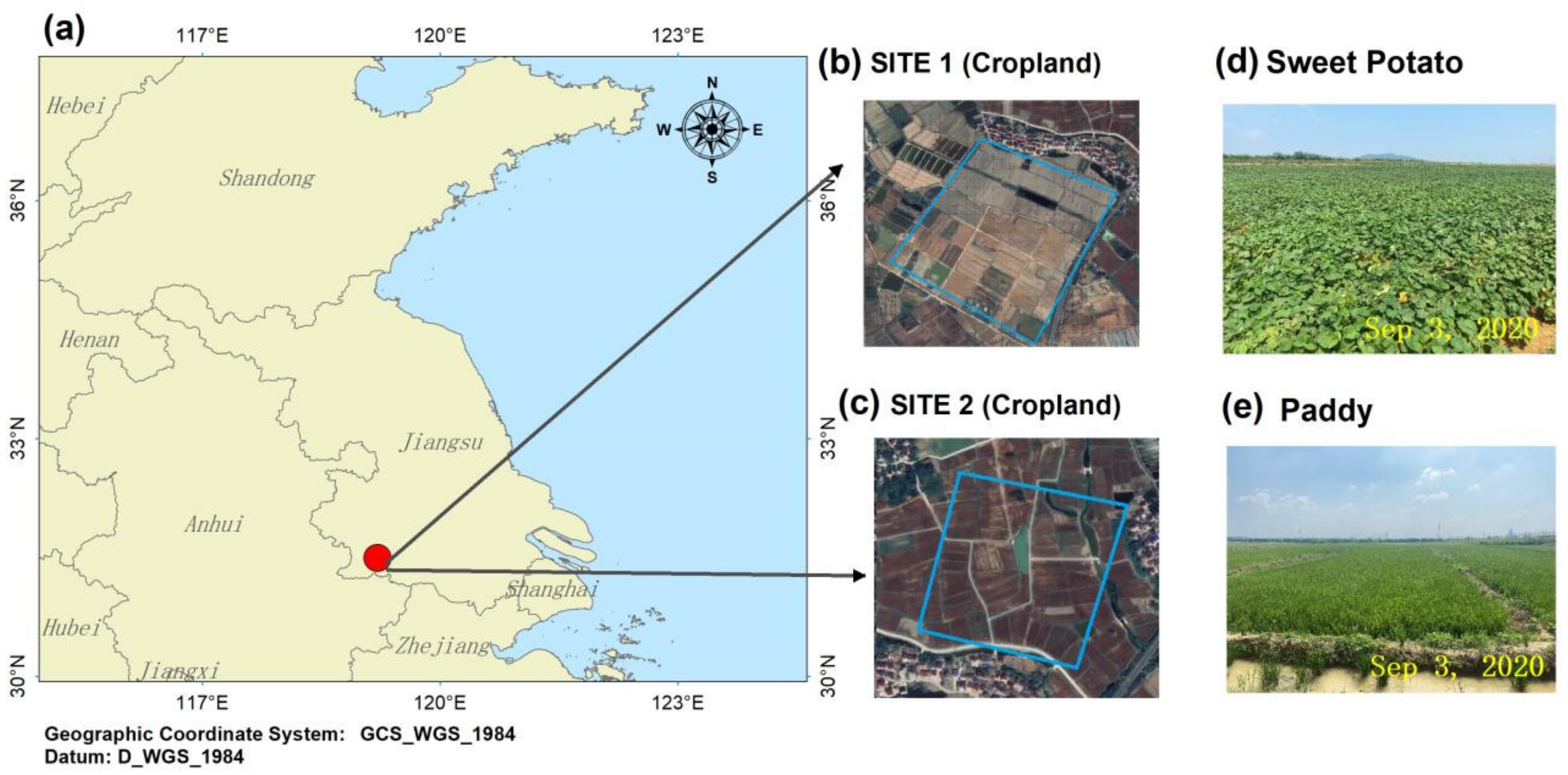
Two heterogeneous experimental sites in this study are located in Liyang City, Jiangsu Province, East China, as shown in Figure 1. The center latitude and longitude of sites 1 and 2 are 119°13′ E, 31°29′58″ N and 119°13′19″ E, 31°30′20″ N, respectively. The extent of each site is about 0.8 km × 0.8 km, corresponding to 640 Sentinel-2 100 m2 pixels. At each experimental site, paddy and potato are the main crops. Paddy is usually transplanted in early June and harvested around mid-November. The potato is sown at the end of May and harvested at the end of November. The peak period of paddy growth is July and August, while the peak period of potato growth is August and September.
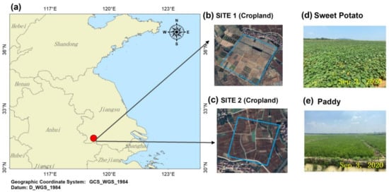
Figure 1.
The location (a) of the two experimental sites in the study area, (b,c) aerial images of two sites from Google Earth, and (d,e) photos of main crops at two sites.
2.2. Generation of NDVI Product from Sentinel-2 Data
The Sentinel-2 constellation, which comprises Sentinel-2A and Sentinel-2B satellites designed by the European Space Agency (ESA), offers free multispectral (spatial resolution from 10 to 60 m) optical imagery at a 5 day interval over global terrestrial surfaces [44]. Due to its high spatiotemporal resolution and rich spectral bands, the Sentinel-2 provides an opportunity for opening a new prospect of generating global VI products at medium and high spatial resolution [6]. In this study, six Sentinel-2 MSI datasets as listed in Table 1 were downloaded from the Copernicus Open Access Hub (https://scihub.copernicus.eu/, accessed on 26 January 2021). Because NDVI is sensitive to atmospheric effects, atmospheric correction of RS images is required before calculating NDVI. The Sentinel-2 Level-2A product in Table 1 provides bottom-of-atmosphere (BOA) corrected reflectance images and it can be directly used to produce the NDVI product. For the Level-1C top-of-atmosphere (TOA) product listed in Table 1, the Sen2Cor algorithm developed by ESA was run through SNAP to correct the Level-1C products from the effects of the atmosphere [45]. Terrain and BRDF-corrections were not considered in this research because the experimental sites and the surrounding area are flat. Based on atmospheric correction data, NIR and RED bands with spatial resolution of 10 m were used for the production of NDVI products.

Table 1.
Overview of RS data used in this study.
3. Methods
The spatial sampling strategy is a fundamental part of data collection for the validation of RS based products [46]. A well-developed sampling strategy is intended to ensure that the data collected are adequately representative and sufficient to generate accurate information about the target population within the available resources. To design a sampling strategy, several elements must be considered: sampling object, sampling approaches, sampling size, and cost of the sampling. All of these elements strictly depend on each other. Sampling size is directly related to sampling cost, sampling object, and sampling approach. In general, if more samples are collected, the information obtained will have higher precision and accuracy. However, more samples also require more money, time, and resources. If the sampling object has greater spatial variation, then more samples are needed. If we choose the optimal sampling approach, fewer observations may be required to achieve a desired level of precision.
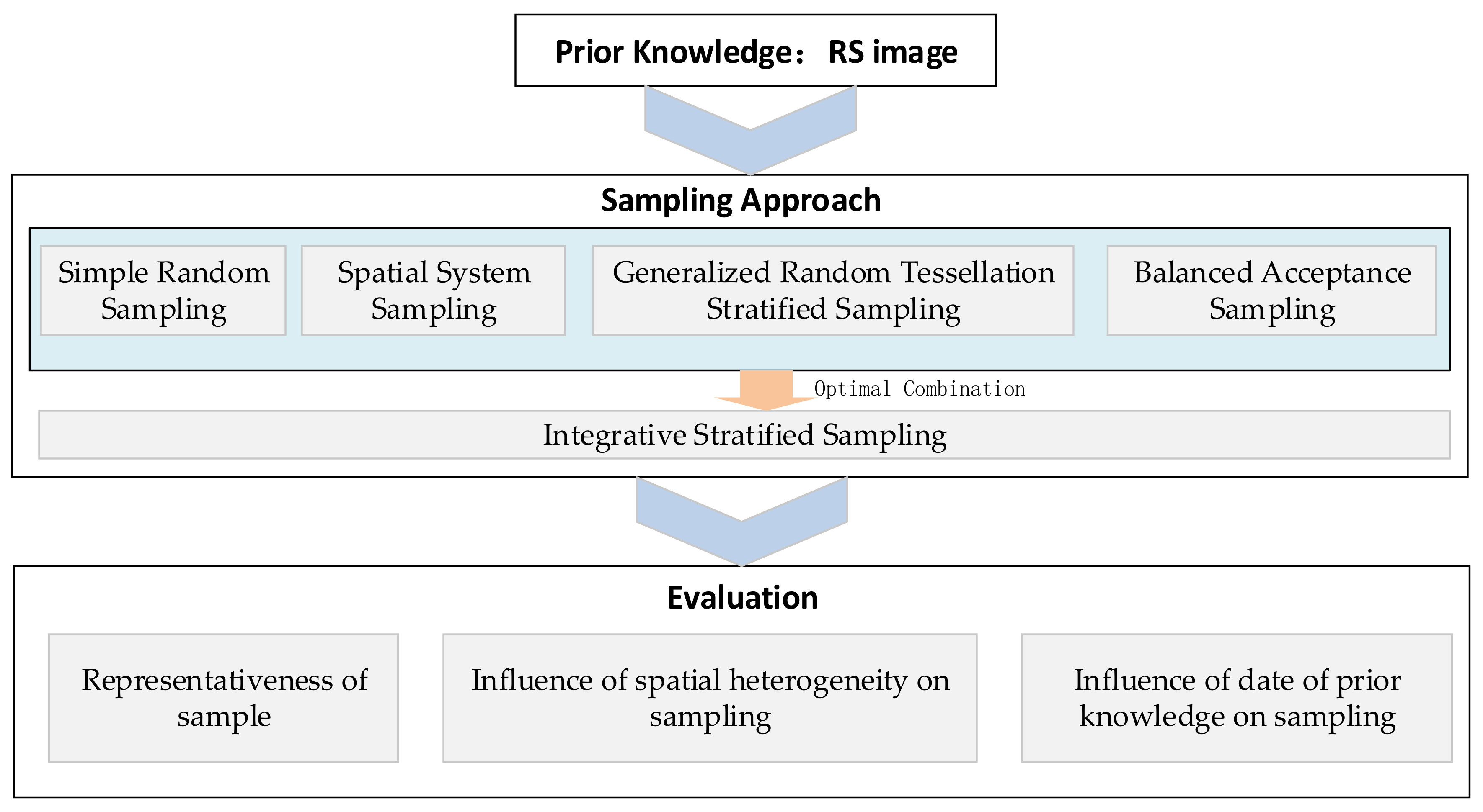
In this paper, we proposed a sampling strategy for a heterogeneous ground surface, based on NDVI data acquired just a few days before the field experiment, as prior knowledge, which then could guide the ground measurement in accordance with the number and location of sampled points from the sampling strategy in the later field campaign. The general flowchart of this approach is shown in Figure 2.
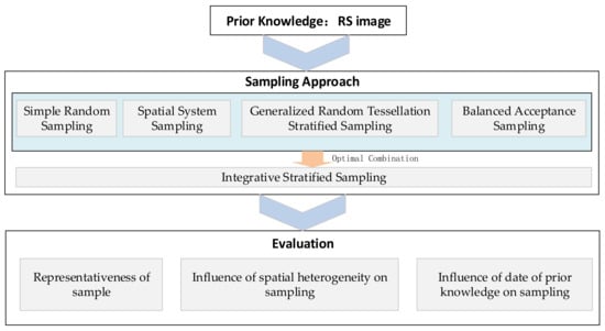
Figure 2.
Flowchart of the approach used in this report.
3.1. Constructing the Integrative Stratified Sampling Approach
For any research, it is essential to choose a sampling method accurately to meet the goals of the study. We all know that due to their own advantages, disadvantages, and applicable conditions, none of the sampling approaches have been proven absolutely superior to the other. Therefore, we proposed an integrative stratified sampling strategy (INTEG-STRAT) whose basic idea is to compare the sampling efficiency of different sampling approaches under different stratification schemes, and then select the optimal combination of sampling method and stratification. In this report, four widely used sampling approaches (SRS, SYS, GRTS, and BAS) in the field of geosciences were selected to construct the integrative stratified sampling strategy applied.
SRS is the most recognized design-based sampling technique [47]. It is a subset of a population in which each member of the subset has an equal probability of being chosen [48]. SYS is also a type of design-based sampling method in which sample members from a larger population are chosen randomly or purposively with a fixed or systematic interval until the desired sample size is reached. The benefits of a systematic approach reside in good spreading of observations over the sampled area. A systematic sample can be considered near perfect spatial balance [32,49]. Spatially balanced sampling is an emerging area in statistical sampling that can be very efficient when the response variable has a strong spatial trend. Several types of spatially balanced sampling methods exist. One of the most frequently-used spatially balanced sampling methods is generalized random tessellation stratified (GRTS), which hierarchically orders a population using a base four numbering scheme and then selects a systematic sample from the ordered population. Balanced acceptance sampling (BAS), similar to GRTS, creates an ordered set of points using the Halton sequence [50,51,52]. The major advantages of GRTS and BAS include their good sample coverage over the entire survey area and good sample representation.
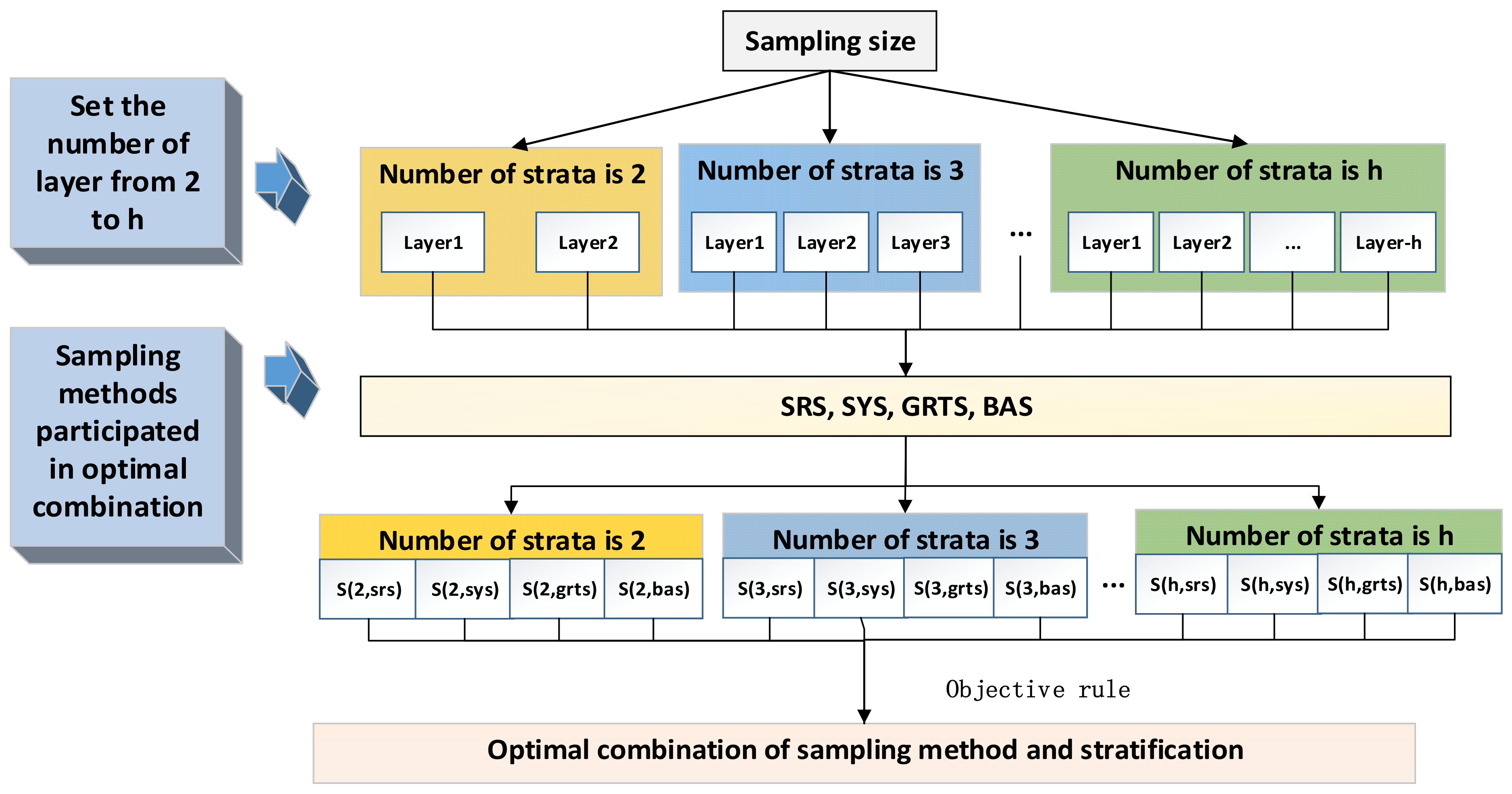
Figure 3 is a flowchart presenting the main steps to conduct sampling for this strategy.

Figure 3.
Flowchart of the approach; S (h, srs) represents the sample points determined by the SRS method when the sample area is divided into h layers.
Step (1). Set the number of samples.
Step (2). Set the range of layers needed to divide the experimental area; for example, from 2 to h, where h represents the maximum number of the layer will be divided. K-means clustering algorithm was used to perform clustering, which uses iterative techniques to group cases in a dataset into clusters that contain similar characteristics.
Step (3). Assign the number of samples to each stratum (layer).
Using Neyman optimal allocation to assign the number of sample to each layer to have the lowest sample variance and the sampling size for stratum h follows:
where is the sample size for stratum h, n is total sample size, is the population size for stratum h, and is the population variance of stratum .
Step (4) Select sampling methods that participate in the process (for example, SRS, SSS, BAS, and GRTS) and determine the spatial location of the sample for each stratum using the different sampling methods.
Step (5) For each sampling method, combine the sample into different strata according to the sampling methods and extract the pixel value of the prior knowledge according to the location of the sample.
Step (6) Interpolate using ordinary kriging (OK) for each set of sampling points, then carry out linear regression and k-fold cross validation with k = 10 folds to evaluate the between estimated values (sample are not included) and the corresponding values on prior knowledge. For spatial interpolation, we use the automap package by Paul Hiemstra for statistical software R, which performs an automatic interpolation by automatically estimating the variogram [53].
Step (7) Select the optimal combination of strata number and sampling method with the minimization of as objective criteria with a certain number of sample.
3.2. Evaluation Approach
3.2.1. Evaluation of Sampling Representativeness and Effectiveness
Relative precision () was used to evaluate the sampling representativeness. Relative precision refers to the ratio of the mean of sample using the particular sampling method (i) relative to the mean of population in the whole study area, which is defined by Formula (2):
In this formula, represents the mean for the ith sampling method and represents the mean for the whole data set within the sampling frame.
In this paper, correlation coefficient and root mean square error () were used to evaluate the effectiveness of the sampling strategy proposed. In the case of small sample size, the data do not necessarily present a normal distribution, but the Pearson correlation coefficient method requires that the data have normal distribution pattern. Therefore, we chose Spearman’s correlation coefficient for correlation analysis, which is defined by Formula (3):
where is the number of data, represents the ith predicted rank of the sample measurement taken on the ith individual, and represents the rank of the NDVI value taken on the ith individual.
where is the number of data, represents the estimated value based on sample points, and represents the corresponding value of image as prior knowledge.
Fisher’s z transformation can be applied to Spearman’s coefficient and then used to estimate the confidence interval (CI) for both correlation coefficients and the differences between two correlations [54,55]. It is most often used to test the significance of the difference between the correlation coefficients of two variables. Fisher’s z transformation applied to is given by Formula (5):
3.2.2. Evaluation of Spatial Heterogeneity on Sampling
In this paper, we explore the influence of spatial heterogeneity on sampling as follows: first, use the semivariogram model to characterize the spatial variability of NDVI calculated from six images listed in Table 1. Then, calculate the sample size when the correlation between the NDVI image and interpolated surface reaches certain accuracy. Last, analyze the relationship between range and sampling size.
The semivariogram is a key and commonly used geostatistical function. Nugget (C0), sill (C), and range (a) are three properties of the model used to describe the spatial characteristic. Nugget represents independent error, measurement error, and/or microscale variation at spatial scales; range represents the distance beyond which the data becomes totally spatially independent, and it can be used as a measure of homogeneity or spatial dependency; sill represents the maximum variability value reached at a distance equal to the range. The principle and formula of semivariograms can be found in other reports [56,57,58].
3.2.3. Evaluation of Influence of Date of Prior Knowledge on Sampling
In order to investigate the impact of the date difference of prior knowledge on the sampling accuracy, we proposed the following steps: (1) Determine the location of sampling points using INTEG-STRAT strategy on the reference NDVI image. (2) Extract NDVI values from all NDVI images according to the location of the sampling points determined in step (1). (3) Perform kriging interpolation using the extracted NDVI values. (4) Calculate and compare the correlation coefficient and between the estimated points and the corresponding pixels on each NDVI images for each day.
4. Results
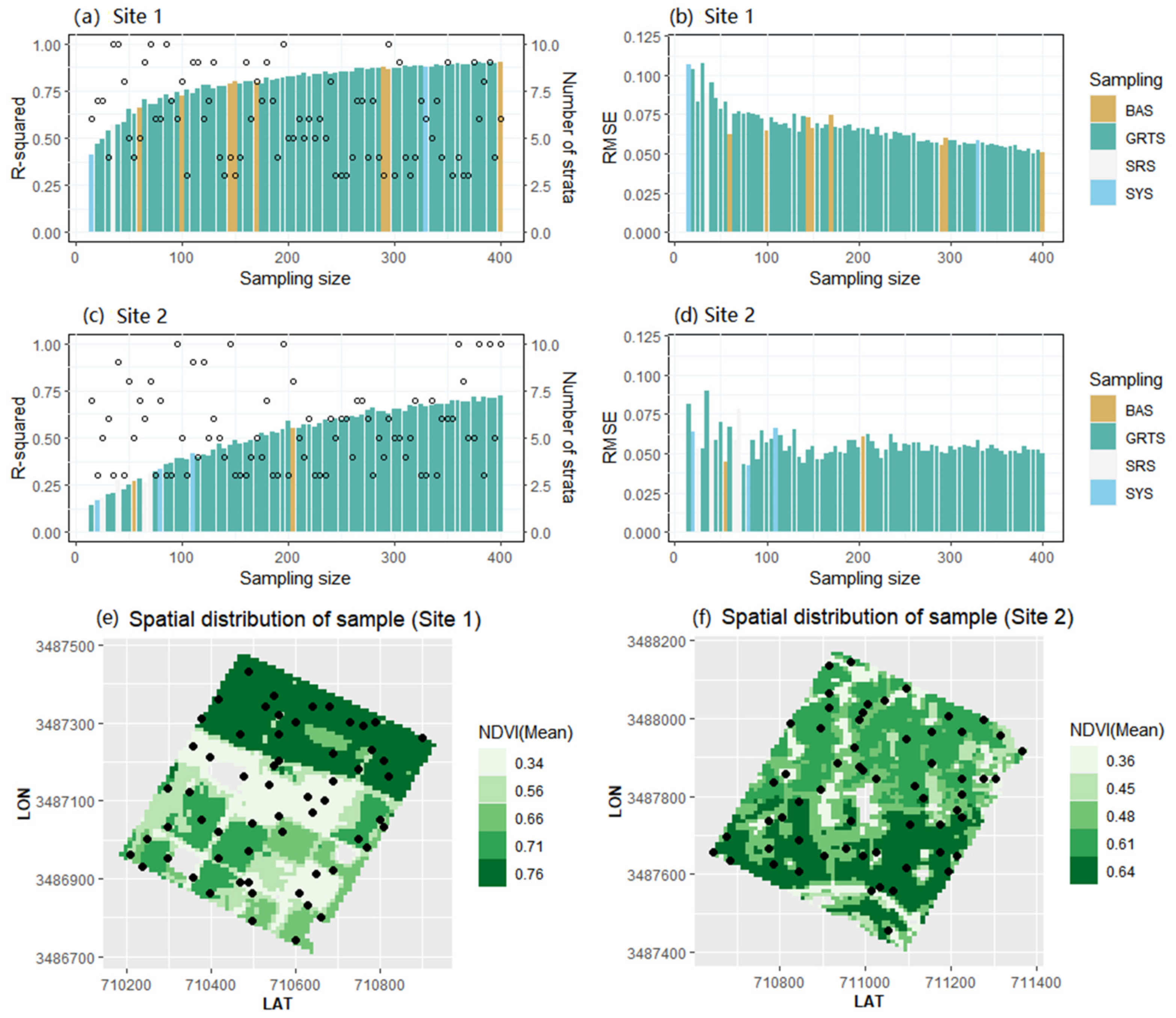
In this part, we conducted sampling experiments on two spatially heterogeneous sites. Figure 4e,f shows the NDVI of the two sites on 5 September 2020. The spatial heterogeneity of NDVI is very obvious, which can be attributed to the different planting structures. At the same time, even for the same crop, there may be spatial heterogeneity due to the difference of crop growth caused by the differences of soil fertility and moisture.
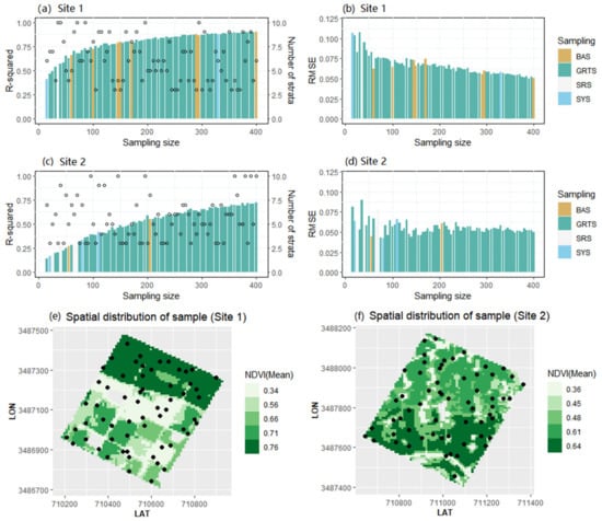
Figure 4.
Sampling result based on INTEG-STRAT strategy: (a–d) represent R-squared and for sites 1 and 2 for different sampling size (the black circles represent numbers of strata and the colors of the bar represent sampling method in the optimal combination determined by INTEG-STRAT strategy); (e,f) shows the distribution of the sample using INTEG-STRAT strategy when sampling size is 60 (the black points represent the spatial location of sample and color scheme represent the clusters stratified using K-means).
The basic parameters in the sampling strategy were set as follows: the sample size ranged from 15 to 400 and the sampling step was 5; the number of strata ranged from 3 to 10, and the k-means technique was used to partition the dataset into K nonoverlapping subgroups (clusters).
Figure 4a,c represents the R-squared obtained through 10-fold cross validation for linear regression between the estimated points and the corresponding pixels of remote sensing product under different sampling size at two sites. The left y-axis represents R-squared, the right y-axis represents the number of strata, and the x-axis represents the sampling size. The height of the bar corresponds to the value of R-squared in the case of optimal combination of sampling method and strata number on different sampling size. The color of bar represents the sampling method in the optimal combination, and the circle points represent the number of strata in this combination. From these figures, note that as the number of samples increases, R-squared gradually increases, but when the number of sample points increases to a certain extent, R-squared tends to be flat. The higher the R-squared, the better the goodness-of-fit between the estimated values and the corresponding values on prior knowledge.
Figure 4b,d represents the between the estimated points and the corresponding pixels of remote sensing product under different sampling size at two sites. is a frequently used measure of the difference between values estimated by a model and the values observed; and is considered as the standard deviation of the residuals (estimation errors). As seen with the increase of sample points, generally showed a downward trend. When the number of sample sites reached 400, of the two sites was around 0.05.
Among the optimal combinations of sampling methods and the number of strata under different sampling numbers, the performance of GRTS is better than that of BAS, SYS, and SSS. At the same time there is no relationship between the number of strata and sampling efficiency. That is to say, a higher the number of layers will not necessarily lead to the improvement of sampling efficiency, and the optimal number of layers must be determined together with the sampling method. Taking the sampling size of 60 as an example, optimal combination of strata number and sampling method with the highest R-squared is five and BAS at site 1, while the optimal combination at site 2 is seven and GRTS. Figure 4e,f shows the spatial distribution of the sample points at two sites.
4.1. Assessment of the Efficiency of the Various Spatial Sampling Strategy
In order to prove the effectiveness of the sampling strategy proposed in this paper, we compared the individual sampling efficiency of GRTS, BAS, SYS, and SSS with the efficiency of the INTEG-STRAT strategy, which could achieve the optimal combination of sampling method and stratification for each sampling size. Sampling efficiency of the various methods was investigated from two aspects: first by comparing sample bias for different sampling approaches and second by comparing the correlation and between the predicted points (sample are not included) and the corresponding values of remote sensing NDVI product.
4.1.1. Comparing the Sampling Representativeness among Different Sampling Strategies
Direct comparison of a ground sample with pixels is a commonly used method in validation of RS-derived products. The sample is a set of measurements taken from a population that is used to describe the characteristics (e.g., mean or variance) of the whole population. The term representativeness of sample is often used to indicate that a sample mirrors a population, which is usually expressed by the difference between the sampling statistics and the population parameters drawn from the sample. In a certain sense, the representativeness is the function of sampling error [59]. A sample without representativeness may not be a reliable source to draw conclusions about the reference population, even if the sample size is very large. Therefore, in order to obtain an accurate and unbiased validation conclusion, the ground sampling points used to participate in the validation must be representative to capture the natural variability of the landscape within the experimental plots. Many researchers showed that using a representative sample, rather than the whole dataset, can effectively balance insight to the quality of the dataset and reduce processing efforts required in validation procedures.
In this part, we use to compare the representativeness of a sample among different sampling strategies. For example, of 2 and 0.8 indicate sampling methods with twice the mean and 80 percent of the mean from the whole population, respectively. In order to minimize the problem of the odd chance of obtaining an unrepresentative sample, which is always possible in any sampling scheme, each of the sampling schemes was simulated 100 times for each sampling size using an R program written by the author. In other words, each simulation was repeated 100 times for each sampling size for each sampling strategy, and the values were averaged together.
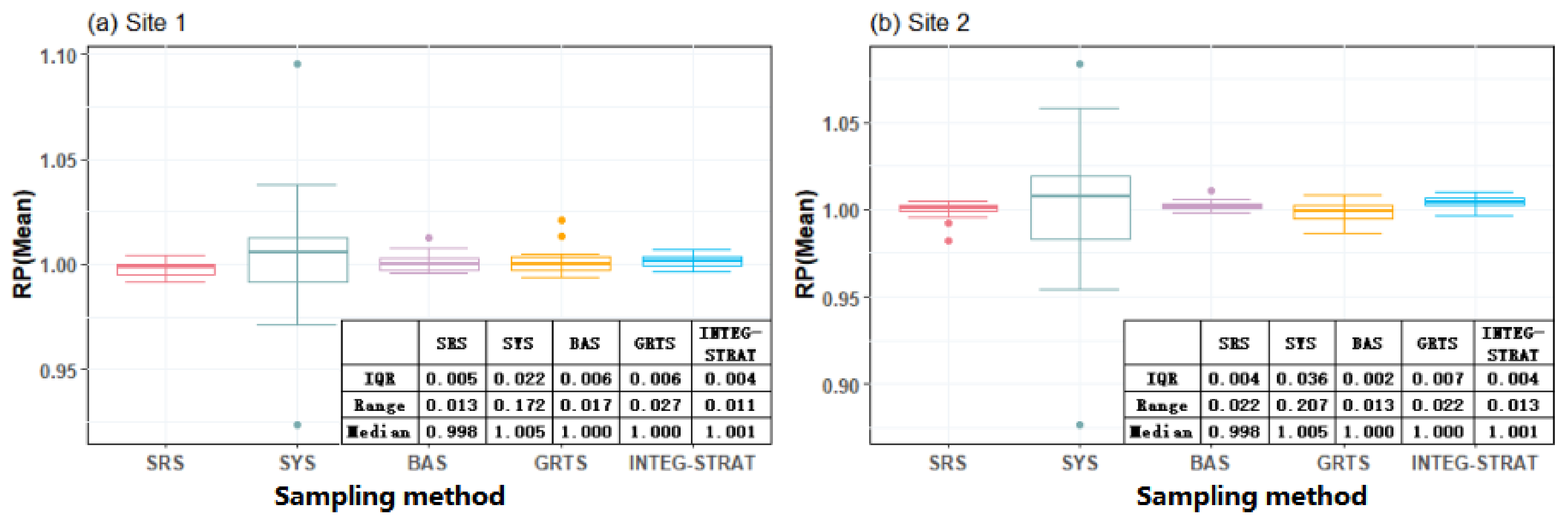
Figure 5 displays the boxplot of averaged of 100 simulations for each sampling method with sampling size from 20 to 200. Boxplot is a standardized way of displaying the distribution of data based on a five number summary, namely minimum, first quartile (Q1), median, third quartile (Q3), and maximum. It reveals outliers and their values. Generally speaking, the box plot of a sample with good representability should have the following characteristics: (1) median value should be close to 1, (2) interquartile range (IQR) should be small, and (3) no outliers. From Figure 5a, we can see the range of calculated based on SRS, SYS, BAS, GRTS, and INTEG-STRAT approaches are 0.013, 0.172, 0.017, 0.027, and 0.011 in site 1, while the range for site 2 are 0.022, 0.0207, 0.013, 0.022, and 0.013, respectively. The representativeness of sampling points obtained by SYS is relatively poor compared with other methods. This conclusion is also applicable to the results of range and IQR. Some researchers have proved that uncertainty greater than 0.02 NDVI are significant [17]. Thus, if using 0.02 NDVI as the uncertainty threshold, we can see that BAS and INTEG-STRAT sampling have a good representativeness at both sites.
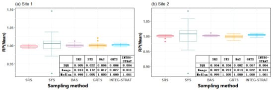
Figure 5.
Boxplot of averaged of 100 simulations for each sampling method with sampling size from 20 to 200: (a,b) represent the for sites 1 and 2, respectively.
4.1.2. Comparing the Correlation and RMSE between the Predicted Surface Based on Sample and NDVI Image
The analysis of representativeness in Section 4.1.1 is based on classical statistical theory, which cannot reflect the spatial representativeness. In this section, we use the correlation and between the estimated points based on sample and the corresponding pixels of NDVI image to explore the efficiency of different sampling methods. Ordinary kriging was used to interpolate the sample points in space, which is a geostatistical interpolation technique that considers both the distance and the degree of variation between known data points when estimating values in unknown areas. Because it requires the fewest assumptions and the least knowledge, it was deemed as the “work horse” of practical geostatistics and will serve in some 90% of cases [60]. Research has shown that kriging would in general be more effective than other methods of interpolation if there is spatial autocorrelation among the sampled data points [61,62,63]. In order to minimize the bias, each of the sampling approaches was performed 100 times.
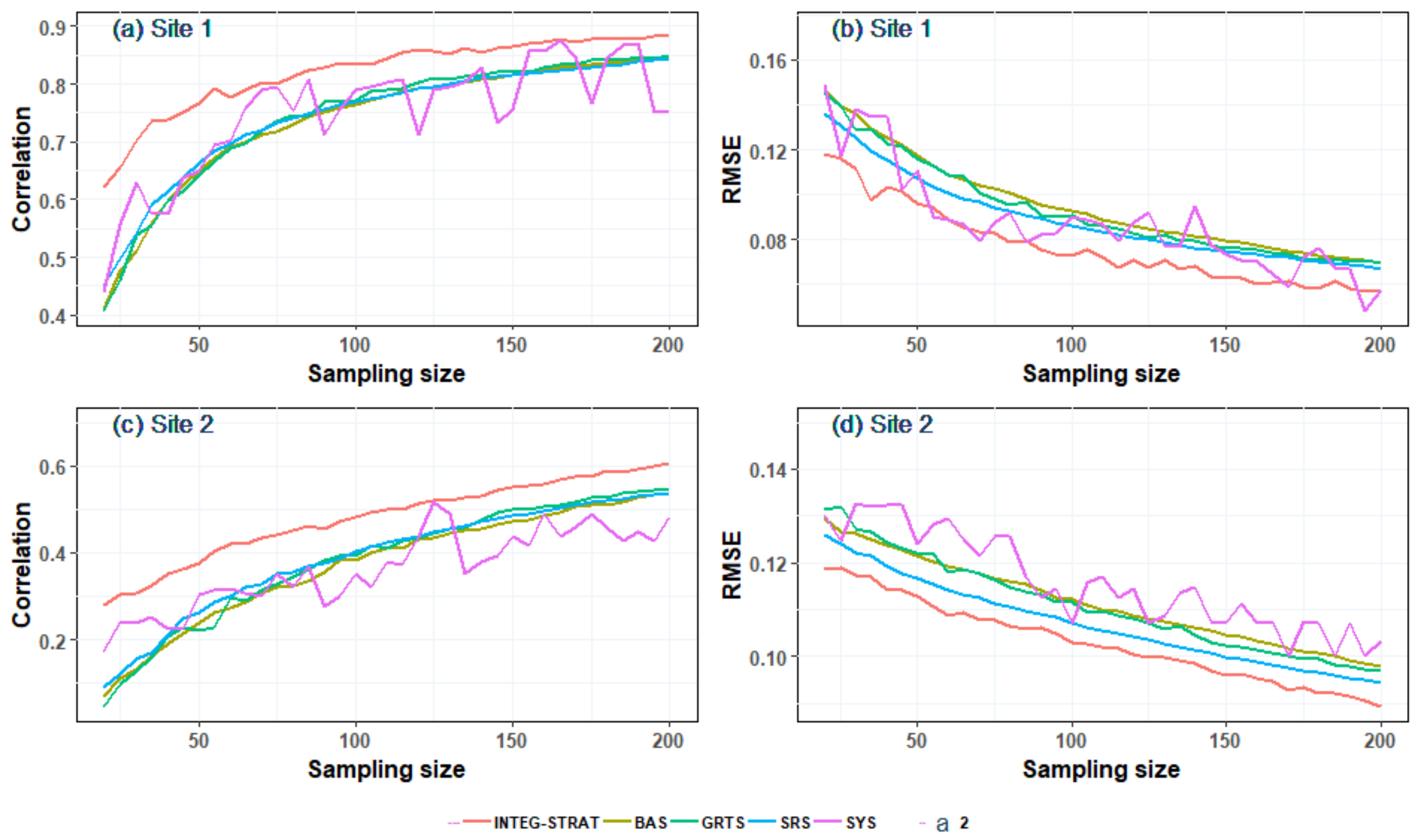
Figure 6 gives the results of the sampling experiments for five sampling strategies at two sites with the correlation coefficient or on the y-axis and the sampling size on the x-axis. From Figure 6a, note that the interpolated surface based on the INTEG-STRAT sample is the best approximation of the NDVI image, compared with the other four methods at site 1. If we want the correlation coefficient between the NDVI image and the simulated NDVI surface to reach 80%, then SRS, BAS, and GRTS require about 130 sampling points while INTEG-STRAT needs only 70 sampling points. The correlation between the NDVI image and the interpolated NDVI surface based on the sample determined by the SYS approach shows a larger variation. Except for the SYS method, with the increase of sampling size, the correlation coefficient shows an increasing trend, and the difference of correlation coefficient between different sampling approaches gradually decreases. Figure 6b shows that the between the RS image and the interpolated NDVI surface generally decreases with increased sampling size, except for the SYS approach. The between the NDVI image and the interpolated surfaces based on the INTEG-STRAT sampling approach is the smallest. From Figure 6c,d, we find that due to the influence of the spatial heterogeneity and spatial autocorrelation of the site, the sampling efficiency of various methods for site 2 is generally low. INTEG-STRAT still presents an advantage, however. Thus, considering the correlation and , we can say that the INTEG-STRAT sampling approach not only has the best sampling efficiency but also has good stability.
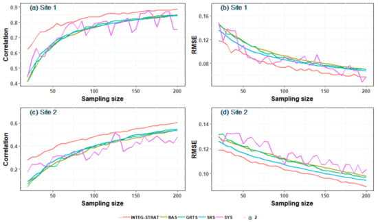
Figure 6.
Comparing of the correlation and between the NDVI image and the interpolated surface: (a,c) correlation and (b,d) at sites 1 and 2, respectively.
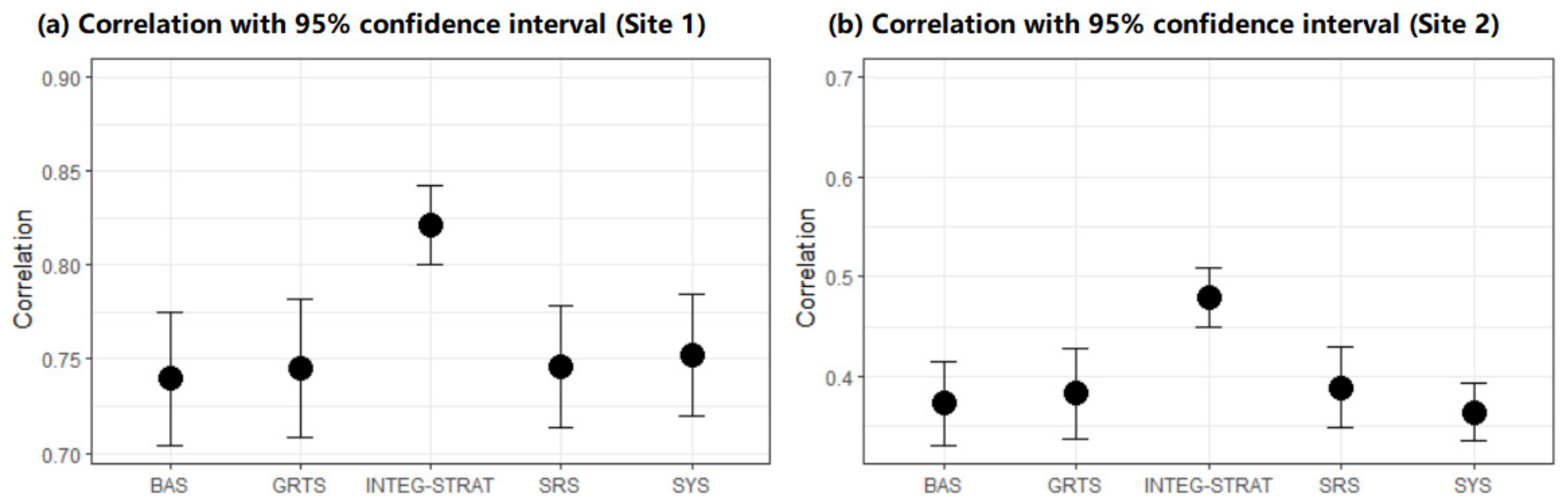
In order to compare correlation coefficients of different sampling strategies, we used Fisher r-to-z transformation to calculate the value of , which can be used to evaluate the significance of the difference between correlations based on different strategies. Figure 7 displays the mean and upper and lower correlation with 95% CI for five strategies with the sampling size ranging from 20 to 200 at both sites. In this paper, the higher mean and upper and lower values of the correlation coefficient indicate a more efficient strategy. The narrower the interval (upper and lower values), the more precise is the strategy. From it, we can see the 95% confidence interval for the correlation based on INTEG-STRAT strategy is (0.800, 0.842) at site 1 and (0.450, 0.510) at site 2, which is obviously narrower and greater than those based on the other four strategies. If we change the CI to 99%, 90%, or even 80%, we can still make the same conclusion. Thus, we can say the INTEG-STRAT strategy is more efficient than the other four.
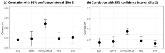
Figure 7.
The mean and upper and lower correlations with 95% CI for five strategies with the sampling size ranging from 20 to 200 at both sites (the black points represent the mean value of correlation coefficients and short horizontal line represents the upper and lower values with 95% CI).
4.2. Influence of Spatial Heterogeneity of the Experimental Site on Sampling
Spatial heterogeneity is one of the most fundamental characteristics of all landscapes. The ideal sampling strategy depends not only on the quantity of the sample, but the location of the sample is also very critical, which depends heavily on the heterogeneity of the variable. This section aims to investigate the effect of spatial heterogeneity on sampling. In order to obtain an overview of the spatial patterns of the experimental sites, we use a semivariogram to investigate the scale and degree of heterogeneity in NDVI over the study sites. Table 2 lists the sill and range of the NDVI images based on Sentinel 2 satellite data and also the number of sampling points required when the correlation between NDVI image and the interpolated surface reaches 70% and 80% by using the INTEG-STRAT sampling approach on six dates. It can be seen that with the increase of range, the number of samples required to meet a certain sampling efficiency decreases gradually. For example, if the range is 143 m, 30 sampling points are needed for the correlation between the NDVI image and the interpolated surface to reach 70%. When the range is reduced to 55 m, 360 sampling points are needed for the correlation to reach 70%.
Table 2.
Sill and range of the NDVI images and the number of sample points required when the sampling efficiency of two sites reaches 70% and 80% at the two sites.
4.3. Influence of Date of Prior Knowledge on Sampling
As noted previously, the efficiency of spatial sampling can be increased by embedding prior knowledge about target population. Conventionally, prior knowledge can be acquired from labor-intensive field-based surveys, which are time consuming, date lagged, and often too expensive and only suitable for small regions. The technology of remote sensing offers a practical and economical means to quantify spatial characteristics of a target domain over large spatial extents. Because of the potential capacity for systematic observations at various scales, many studies began to use remote sensing data to acquire prior knowledge that gives useful information for sampling. In recent years, with the shortening of the revisit period of medium and high spatial resolution satellite data, it is possible to use the same kind of satellite data acquired before the ground campaign as prior knowledge to design the sampling strategy for validation of RS-derived vegetation products.
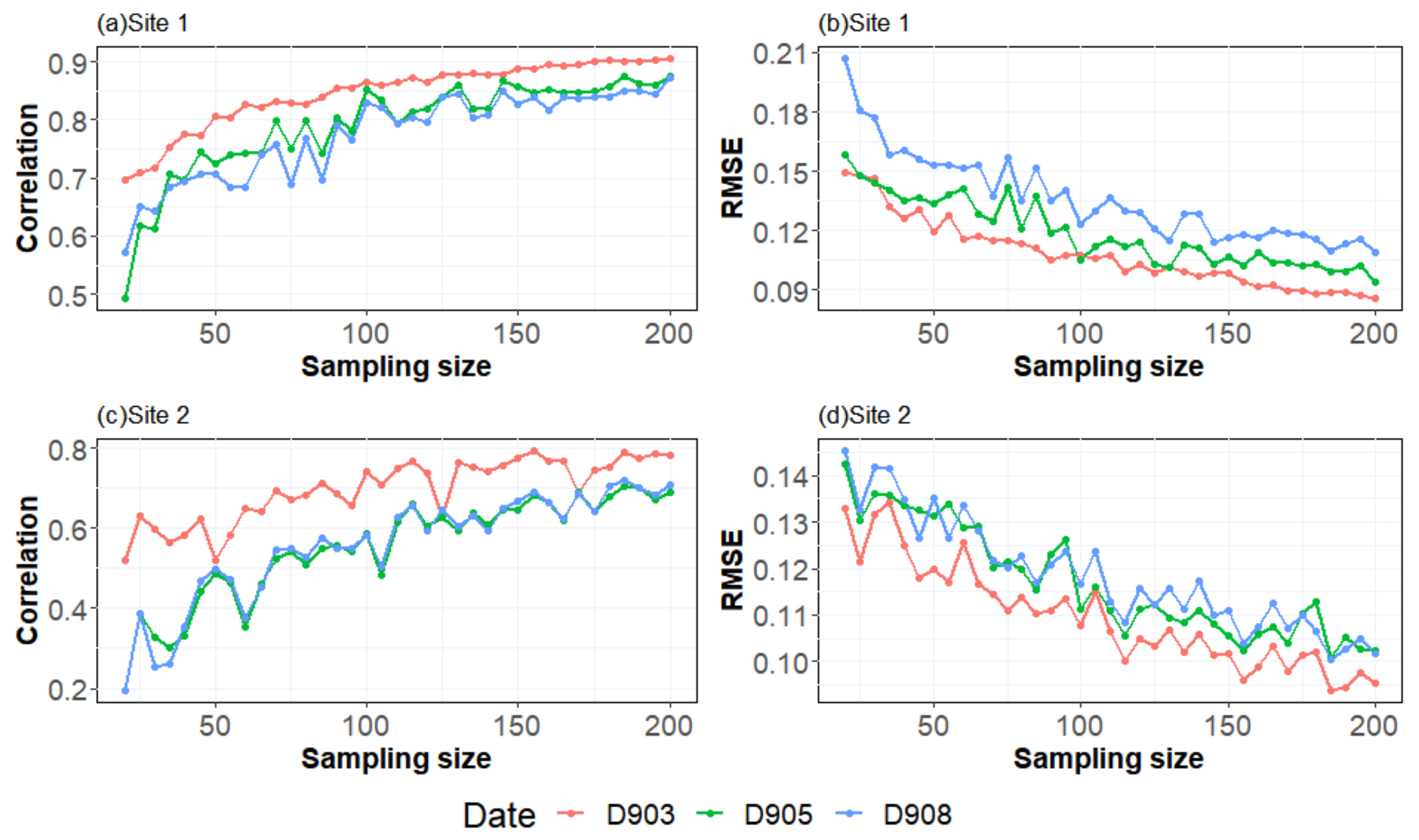
In this section, we follow the steps in Section 3.2.3 to investigate the impact of the date difference of prior knowledge on the sampling accuracy based on three scenes of Sentinel data for 3, 5, and 8 September 2020 at two experiment sites. In this case, we used NDVI of 3 September as reference data; the result is shown in Figure 8. The red lines in Figure 8 represent the correlation/ between the NDVI image on 3 September and the interpolated surface based on a sample taken under different sampling sizes. The green lines represent the correlation/ between the NDVI image on 5 September and interpolated surface based on a sample selected from the NDVI image on 5 September, while the blue lines represent the correlation/ between the NDVI image on 8 September and the interpolated surface based on a sample selected from NDVI image on 8 September. By comparing the three lines, we can see the effect of differences in the NDVI image induced by crop growth on the sampling efficiency. For both sites 1 and 2, the difference between the red and green lines is general smaller than that between the red and blue lines, which indicate the sampling strategy based on the 3 September images has a better performance on the images of 5 September than on the 8 September images.
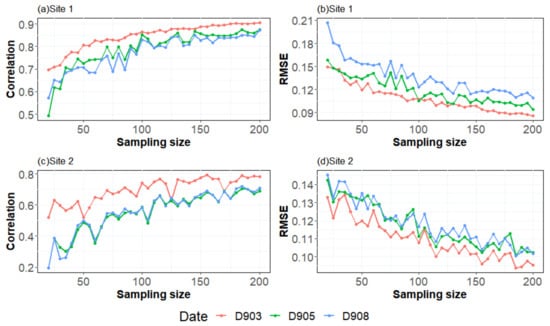
Figure 8.
The correlation and between NDVI images on 3, 5, and 8 September and the predicted surface using the sampling points chosen, based on prior knowledge for 3 September: (a,c) correlation and (b,d) for the two sites.
In this section, we used Fisher r-to-z transformation to evaluate the significance of the difference between correlations on different dates. From Figure 9, we can see a 95% confidence interval of the correlation coefficients between NDVI images and the predicted surface using the sampling points chosen based on prior knowledge: (0.827, 0.864) on 3 September, (0.763, 0.817) on 5 September, and (0.750, 0.800) on 8 September at site 1. If the sampling strategy based on the prior knowledge of 3 September is adopted for the images on 5 September, the mean correlation coefficient decreases by about 5.6%. If it were used for the 5 September image, the correlation would drop by about 7.1 percent.
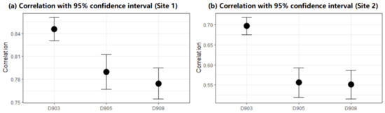
Figure 9.
The mean and upper and lower correlations with 95% CI for INTEG-STRAT strategy with the sampling size ranging from 20 to 200 on three dates ((a) is for site 1 and (b) is for site 2. The black points represent the mean value of correlation coefficients and short horizontal lines represent the upper and lower values with 95% CI).
5. Discussion
With the rapid development of RS technology, rich kinds of RS products are available for geosciences. However, many studies indicated that some RS products might overestimate/underestimate the accuracy of target variables [64,65]. Therefore, validation with ground observation data is deemed as the fundamental task to promote the application of RS products. How to design an efficient sampling strategy to guarantee the accuracy and reliability of the validation result is one of key scientific issues in the validation stage. At present, spatial random sampling, spatial system sampling, convenient sampling, and arbitrary sampling are widely used methods in many validation activities for RS products. In fact, a suitable sampling strategy should be designed according to the particular characteristics of the selected region. If the target variables are homogeneous, then all of the methods noted can perform well. Otherwise, sampling strategies that consider the spatial stratification are recommended. Some research has demonstrated that effective strata based on some prior information can greatly reduce the uncertainty of the sampling [27,36,37]. How to determine the effective stratification is an important issue. For example, means of a surface with heterogeneity (MSN) is a sampling strategy by taking both spatial autocorrelation and spatial stratified heterogeneity into account [26,30]. In MSN, the principle of stratification is to maximize the variance between strata and minimize the variance within strata. Based on the strata map, the simulated annealing algorithm is used to optimize the locations of sampling points to minimize the mean squared estimation error criteria. From Figure 4, we find that the efficiency of different sampling methods varies greatly under the same stratification, and the effective stratification is the comprehensive result of spatially heterogeneous sampling points and the sampling approach; it should not be a fixed number. Therefore, we put forward a new sampling strategy whose basic idea is to achieve the optimal combination of optimal sampling methods and stratification considering the heterogeneity of the experimental sites based on the RS-based prior knowledge.
How to choose a sample size is another important problem in sampling. Due to the variability of a heterogeneous surface, a sufficient sample size must be collected in order to obtain a value that is representative of the experimental sites. For the validation of RS products, values for all pixels of RS products should be collected in order to guarantee the reliability of the validation. Due to time and labor cost, however, this solution is not feasible. Currently, there is no accepted quantitative method to determine the sampling size. Through the research presented herein, we find that at different sites, the number of sampling points required to achieve a certain sampling accuracy is very different. For example, in the case of site 2, if the correlation between the interpolated surface and the NDVI image on 5 September reaches 70%, then 355 samples must be collected, while at site 1 only 30 sample are needed. Therefore, it is very important to carry out presampling based on prior knowledge; we can find the optimal number of samples at a certain level of accuracy, thereby providing a reliability analysis for our validation conclusions.
Comparing to existing studies about sampling methods, our strategy was demonstrated to be more reliable and can better capture the spatial surface heterogeneity when compared to random or other sampling methods. INTEG-STRAT has limitations. Through the analysis presented herein, we find that the date interval between the prior knowledge and the ground campaign is an important issue that affects the accuracy of the validation result. In validation, one frequently asked question is, what is the date interval between the prior knowledge and ground campaign to ensure the accuracy of the validation? In fact, many analysts directly use data that are a few days apart from ground activities as prior knowledge. From this paper, we can see that as the date interval increases, the efficiency of the sampling strategy decreases. In fact, this can be explained by differences in the rate of vegetation growth in different periods. Application of INTEG-STRAT is limited if the vegetation is rapidly increasing or decreasing. Therefore, when designing a sampling strategy based on prior knowledge, it is necessary to first analyze and then determine the size of the date window with a certain confidence interval, and then select appropriate data according to the date window as prior knowledge. In the future, we plan to build a model to calculate an ideal date window size given desired levels of precision and confidence for typical vegetation based on long-term observation data from a ground-based wireless sensor network.
Based on our study, we propose the following steps to use INTEG-STRAT sampling strategy to guide the collection of ground data for the validation of a RS product: (1) calculate VIs from a high-resolution image of the validation sites close to the ground campaign, (2) perform the INTEG-STRAT sampling on the image, (3) take ground measurements of VIs in accordance with the number and location of sampled points from step (2), and (4) estimate the accuracy of the RS products based on the ground measurements.
6. Conclusions
There is a clear requirement for remote sensing VI products with medium and high spatial resolution to be validated using reference data, such as in situ measurements, due to VIs’ significant role in validating coarse resolution products, together with modeling the ecological environment at local scale. Sampling strategy is one of the important factors to ensure the success of ground validation activities. In this paper, we proposed an integrative stratified sampling strategy based on NDVI data as the prior knowledge. The performance of the sampling strategy was investigated at two heterogeneous sites located in Liyang city in China. By comparing the individual sampling efficiency of GRTS, BAS, SYS, and SSS with the efficiency of the INTEG-STRAT strategy, which could achieve the optimal combination of the sampling method and stratification, we find that (1) INTEG-STRAT requires fewer samples to become stable and has higher accuracy, (2) the samples from INTEG-STRAT are spread across geographical space and are representative, and (3) INTEG-STRAT can perform well if there are small differences between the NDVI data used as prior knowledge and those acquired during the ground campaign. In general, the sampling design proposed will support validation activities to locate the sampling points for the field measurements.
It must be mentioned that lacking in situ evaluation of the INTEG-STRAT sampling strategy is a weakness of this paper. In the next step, we will carry out evaluation based on the ground campaign.
Author Contributions
Conceptualization, T.L., X.Z. and Z.T.; methodology, T.L.; software, X.S.; validation, X.Z., Z.T. and X.S.; formal analysis, T.L., J.W., R.L. and F.X.; data curation, J.W.; writing—original draft, T.L.; writing—review and editing, T.L., X.Z. and Z.T.; visualization, X.S.; funding acquisition, X.Z. All authors have read and agreed to the published version of the manuscript.
Funding
This paper was granted by the Joint Validation of Multi-source Remote Sensing Information and Sharing in BRICS Countries, under contract No. 2018YFE0124200 (National Key R&D Program of China), and the Key Technologies for Collaborative Processing and Joint Verification of Basic Common Products of Quantitative Remote Sensing for the “Belt and Road” under contract No. 2020YFE0200700 (National Key R&D Program of China).
Institutional Review Board Statement
Not applicable.
Informed Consent Statement
Not applicable.
Data Availability Statement
The satellite data used in this study are public domain, available from ESA (https://scihub.copernicus.eu/dhus/#/home, last accessed on 26 January 2021). Other data that support the findings of this study are available from the author upon reasonable request.
Acknowledgments
We would like to thank R package for helping us to design the sampling strategy and perform data analysis and plotting.We also thank the journal’s editors and reviewers for providing insightful comments and suggestions for this paper.
Conflicts of Interest
The authors declare no conflict of interest.
References
- Srivastava, A.; Kumari, N.; Maza, M. Hydrological Response to Agricultural Land Use Heterogeneity Using Variable Infiltration Capacity Model. Water Resour. Manag. 2020, 34, 3779–3794. [Google Scholar] [CrossRef]
- Maza, M.; Srivastava, A.; Bisht, D.S.; Raghuwanshi, N.S.; Bandyopadhyay, A.; Chatterjee, C.; Bhadra, A. Simulating the hydrological response of a monsoon dominated reservoir catchment and command with heterogeneous cropping pattern using VIC model. J. Earth Syst. Sci. 2020, 129, 1–16. [Google Scholar] [CrossRef]
- Huete, A.; Didan, K.; van Leeuwen, W.; Miura, T.; Glenn, E. MODIS Vegetation Indices. In Land Remote Sensing and Global Environmental Change: NASA’s Earth Observing System and the Science of ASTER and MODIS; Ramachandran, B., Justice, C.O., Abrams, M.J., Eds.; Springer: New York, NY, USA, 2011; pp. 579–602. [Google Scholar]
- Beck, P.S.A.; Atzberger, C.; Høgda, K.A.; Johansen, B.; Skidmore, A.K. Improved monitoring of vegetation dynamics at very high latitudes: A new method using MODIS NDVI. Remote Sens. Environ. 2006, 100, 321–334. [Google Scholar] [CrossRef]
- Sun, K.; Chen, X.; Zhu, Z.; Zhang, T. High Resolution Aerosol Optical Depth Retrieval Using Gaofen-1 WFV Camera Data. Remote Sens. 2017, 9, 89. [Google Scholar] [CrossRef] [Green Version]
- Zhang, T.; Su, J.; Liu, C.; Chen, W.-H.; Liu, H.; Liu, G. Band Selection in Sentinel-2 Satellite for Agriculture Applications. In Proceedings of the 2017 23rd International Conference on Automation and Computing (ICAC), Huddersfield, UK, 7–8 September 2017. [Google Scholar] [CrossRef] [Green Version]
- Hu, Q.; Yang, J.; Xu, B.; Huang, J.; Memon, M.S.; Yin, G.; Zeng, Y.; Zhao, J.; Liu, K. Evaluation of Global Decametric-Resolution LAI, FAPAR and FVC Estimates Derived from Sentinel-2 Imagery. Remote Sens. 2020, 12, 912. [Google Scholar] [CrossRef] [Green Version]
- Global Climate Observing System. The Global Observing System for Climate: Implementation Needs. In GCOS Steering Committee at Their 24th Meeting in Guayaquil, Ecuador, in October 2016. 2016. Available online: https://unfccc.int/sites/default/files/gcos_ip_10oct2016.pdf (accessed on 10 January 2021).
- Herold, M.; Carter, S.; Avitabile, V.; Espejo, A.B.; Jonckheere, I.; Lucas, R.; McRoberts, R.E.; Næsset, E.; Nightingale, J.; Petersen, R.; et al. The Role and Need for Space-Based Forest Biomass-Related Measurements in Environmental Management and Policy. Surv. Geophys. 2019, 40, 757–778. [Google Scholar] [CrossRef] [Green Version]
- Djamai, N.; Fernandes, R.; Weiss, M.; McNairn, H.; Goïta, K. Validation of the Sentinel Simplified Level 2 Product Prototype Processor (SL2P) for mapping cropland biophysical variables using Sentinel-2/MSI and Landsat-8/OLI data. Remote Sens. Environ. 2019, 225, 416–430. [Google Scholar] [CrossRef]
- Group on Earth Observations. Global Agricultural Monitoring Initiative. Stocktaking Overview of the G20 Global Agricultural Monitoring (GEOGLAM) Initiative since the Inception of the 2011 Action Plan on Food Price Volatility. 2018. Available online: https://www.earthobservations.org/geoglam_resources/1%20Home/Planning%20and%20Reporting/G20%20Stocktaking%202018%20Argentina.pdf (accessed on 10 January 2021).
- Heinzel, V.; Franke, J.; Menz, G. Assessment of cross-sensor NDVI-variations caused by spectral band characteristics. In Proceedings of the Remote Sensing and Modeling of Ecosystems for Sustainability III, San Diego, CA, USA, 13–17 August 2006; Volume 6298. [Google Scholar]
- Brown, M.E.; Pinzon, J.E.; Didan, K.; Morisette, J.T.; Tucker, C.J. Evaluation of the consistency of long-term NDVI time series derived from AVHRR, SPOT-vegetation, SeaWiFS, MODIS, and Landsat ETM+ sensors. IEEE Trans. Geosci. Remote Sens. 2006, 44, 1787–1793. [Google Scholar] [CrossRef]
- Van Leeuwen, W.J.D.; Orr, B.J.; Marsh, S.E.; Herrmann, S.M. Multi-sensor NDVI data continuity: Uncertainties and implications for vegetation monitoring applications. Remote Sens. Environ. 2006, 100, 67–81. [Google Scholar] [CrossRef]
- Ke, Y.; Im, J.; Lee, J.; Gong, H.; Ryu, Y. Characteristics of Landsat 8 OLI-derived NDVI by comparison with multiple satellite sensors and in-situ observations. Remote Sens. Environ. 2015, 164, 298–313. [Google Scholar] [CrossRef]
- Teillet, P.M.; Ren, X. Spectral band difference effects on vegetation infices derived from multiple satellite sensor data. Can. J. Remote Sens. 2008, 34, 159–173. [Google Scholar]
- Borgogno-Mondino, E.; Lessio, A.; Gomarasca, M.A. A fast operative method for NDVI uncertainty estimation and its role in vegetation analysis. Eur. J. Remote Sens. 2016, 49, 137–156. [Google Scholar] [CrossRef]
- Justice, C.; Belward, A.; Morisette, J.; Lewis, P.; Privette, J.; Baret, F. Developments in the ‘validation’ of satellite sensor products for the study of the land surface. Int. J. Remote Sens. 2000, 21, 3383–3390. [Google Scholar] [CrossRef]
- Zhang, R.; Tian, J.; Li, Z.; Su, H.; Chen, S.; Tang, X. Principles and methods for the validation of quantitative remote sensing products. Sci. China Earth Sci. 2010, 53, 741–751. [Google Scholar] [CrossRef]
- Otto, J.; Brown, C.; Buontempo, C.; Doblas-Reyes, F.; Jacob, D.; Juckes, M.; Keup-Thiel, E.; Kurnik, B.; Schulz, J.; Taylor, A.; et al. Uncertainty: Lessons learned for climate services. Bull. Am. Meteorol. Soc. 2017, 97, S265–S269. [Google Scholar] [CrossRef] [Green Version]
- Loew, A.; Bell, W.; Brocca, L.; Bulgin, C.E.; Burdanowitz, J.; Calbet, X.; Donner, R.V.; Ghent, D.; Gruber, A.; Kaminski, T.; et al. Validation practices for satellite-based Earth observation data across communities. Rev. Geophys. 2017, 55, 779–817. [Google Scholar] [CrossRef] [Green Version]
- Wu, X.; Xiao, Q.; Wen, J.; You, D.; Hueni, A. Advances in quantitative remote sensing product validation: Overview and current status. Earth Sci. Rev. 2019, 196, 102875. [Google Scholar] [CrossRef]
- Soto-Berelov, M.; Jones, S.; Farmer, E.; Woodgate, W. Review of validation standards of biophysical Earth Observation products. In AusCover Good Practice Guidelines: A Technical Handbook Supporting Calibration and Validation Activities of Remotely Sensed Data Product; Held, A., Phinn, S., Soto-Berelov, M., Jones, S., Eds.; TERN AusCover: Brisbane, Australia, 2015; pp. 8–30, Chapter 2; ISBN 978-0-646-94137-0. [Google Scholar]
- Schneider, P.; Ghent, D.; Corlett, G.; Prata, F.; Remedios, J. AATSR Validation: LST Validation Protocol; University of Leicester: Leicester, UK, 2012; pp. 1–39. [Google Scholar]
- Martin, M.A.; Ghent, D.; Pires, A.C.; Göttsche, F.; Cermak, J.; Remedios, J.J. Comprehensive in situ validation of five satellite land surface temperature data sets over multiple stations and years. Remote Sens. 2019, 11, 479. [Google Scholar] [CrossRef] [Green Version]
- Ding, Y.; Ge, Y.; Hu, M.; Wang, J.; Wang, J.; Zheng, X.; Zhao, K. Comparison of spatial sampling strategies for ground sampling and validation of MODIS LAI products. Int. J. Remote Sens. 2014, 35, 7230–7244. [Google Scholar] [CrossRef]
- Cao, Z.; Wang, J.; Li, L.; Jiang, C. Strata Efficiency and Optimization strategy of Stratified Sampling on Spatial Population. Prog. Geogr. 2008, 27, 152–160. [Google Scholar]
- Tian, Y.; Woodcock, C.E.; Wang, Y.; Privette, J.L.; Shabanov, N.V.; Zhou, L.; Zhang, Y.; Buermann, W.; Dong, J.; Veikkanen, B.; et al. Multiscale analysis and validation of the MODIS LAI product: II. Sampling strategy. Remote Sens. Environ. 2002, 83, 431–441. [Google Scholar] [CrossRef]
- Yin, G.; Li, A.; Verger, A. Spatiotemporally Representative and Cost-Efficient Sampling Design for Validation Activities in Wanglang Experimental Site. Remote Sens. 2017, 9, 1217. [Google Scholar] [CrossRef] [Green Version]
- Wang, J.; George, C.; Hu, M. Modeling Spatial Means of Surfaces with Stratified Nonhomogeneity. IEEE Trans. Geosci. Remote Sens. 2009, 47, 4167–4174. [Google Scholar] [CrossRef]
- Wang, J.; Li, L.; George, C. Sampling and Kriging Spatial Means: Efficiency and Conditions. Sensors 2009, 9, 5224–5240. [Google Scholar] [CrossRef]
- Wang, J.; Stein, A.; Gao, B.; Ge, Y. A review of spatial sampling. Spat. Stat. 2012, 2, 1–14. [Google Scholar] [CrossRef]
- Wang, J.; Ge, Y.; Heuvelink, G.B.; Zhou, C. Spatial Sampling Design for Estimating Regional GPP with Spatial Heterogeneities. IEEE Geosci. Remote Sens. Lett. 2014, 11, 539–543. [Google Scholar] [CrossRef]
- Castaldi, F.; Chabrillat, S.; van Wesemael, B. Sampling Strategies for Soil Property Mapping Using Multispectral Sentinel-2 and Hyperspectral EnMAP Satellite Data. Remote Sens. 2019, 11, 309. [Google Scholar] [CrossRef] [Green Version]
- Wang, J.; Haining, R.; Cao, Z. Sample surveying to estimate the mean of a heterogeneous surface: Reducing the error variance through zoning. Int. J. Geogr. Inf. Sci. 2010, 24, 523–543. [Google Scholar] [CrossRef]
- Zeng, Y.; Li, J.; Liu, Q.; Qu, Y.; Huete, A.; Xu, B.; Yin, G.; Zhao, J. An optimal sampling design for observing and validating long-term leaf area index with temporal variations in spatial heterogeneities. Remote Sens. 2015, 7, 1300–1319. [Google Scholar] [CrossRef] [Green Version]
- Zeng, Y.; Li, J.; Liu, Q.; Li, L.; Xu, B.; Yin, G.; Peng, J. A Sampling Strategy for Remotely Sensed LAI Product Validation over Heterogeneous Land Surfaces. IEEE J. Sel. Top. Appl. Earth Obs. Remote Sens. 2014, 7, 3128–3142. [Google Scholar] [CrossRef]
- Woodgate, W.; Soto-Berelov, M.; Suarez, L.; Jones, S.; Hill, M.; Wilkes, P.; Axelsson, C.; Haywood, A.; Mellor, A. Searching for the Optimal Sampling Design for Measuring LAI in an Upland Rainforest. In Proceedings of the Geospatial Science Research Symposium GSR2, Melbourne, Australia, 10–12 December 2012; ISBN 978-0-9872527-1-5. [Google Scholar]
- Morisette, J.T.; Baret, F.; Privette, J.L.; Myneni, R.B.; Nickeson, J.E.; Garrigues, S.; Shabanov, N.V.; Weiss, M.; Fernandes, R.A.; Leblanc, S.G.; et al. Validation of global moderate-resolution LAI products: A framework proposed within the CEOS land product validation subgroup. IEEE Trans. Geosci. Remote Sens. 2006, 44, 1804–1814. [Google Scholar] [CrossRef] [Green Version]
- Cohen, W.B.; Justice, C.O. Validating MODIS Terrestrial Ecology Products: Linking In Situ and Satellite Measurements. Remote Sens. Environ. 1999, 70, 1–3. [Google Scholar] [CrossRef]
- Wang, Z.; Schaaf, C.B.; Strahler, A.H.; Chopping, M.J.; Román, M.O.; Shuai, Y.; Woodcock, C.E.; Hollinger, D.Y.; Fitzjarrald, D.R. Evaluation of MODIS albedo product (MCD43A) over grassland, agriculture and forest surface types during dormant and snow-covered periods. Remote Sens. Environ. 2014, 140, 60–77. [Google Scholar] [CrossRef] [Green Version]
- Román, M.O.; Gatebe, C.K.; Shuai, Y.; Wang, Z.; Gao, F.; Masek, J.G.; Liang, S.; Schaaf, C.B.; Schaaf, C.B. Use of In Situ and Airborne Multiangle Data to Assess MODIS- and Landsat-Based Estimates of Directional Reflectance and Albedo. IEEE Trans. Geosci. Remote Sens. 2013, 51, 1393–1404. [Google Scholar] [CrossRef]
- Román, M.O.; Schaaf, C.B.; Lewis, P.; Gao, F.; Anderson, G.P.; Privette, J.L.; Strahler, A.H.; Woodcock, C.E.; Barnsley, M. Assessing the coupling between surface albedo derived from MODIS and the fraction of diffuse skylight over spatially-characterized landscapes. Remote Sens. Environ. 2010, 114, 738–760. [Google Scholar] [CrossRef]
- Drusch, M.; del Bello, U.; Carlier, S.; Colin, O.; Fernandez, V.; Gascon, F.; Hoersch, B.; Isola, C.; Laberinti, P.; Martimort, P.; et al. Sentinel-2: ESA’s Optical High-Resolution Mission for GMES Operational Services. Remote Sens. Environ. 2012, 120, 25–36. [Google Scholar] [CrossRef]
- Magdalena, M.; Bringfried, P.; Jerome, L.; Vincent, D.; Uwe, M.; Ferran, G. Sen2Cor for Sentinel-2. In Proceedings of the Image and Signal Processing for Remote Sensing XXIII, Warsaw, Poland, 11–14 September 2017; Volume 10427. [Google Scholar] [CrossRef] [Green Version]
- Wang, Y.; Jiang, L.; Qi, Q.; Ying, L.; Wang, J. Remote Sensing-Guided Sampling Design with Both Good Spatial Coverage and Feature Space Coverage for Accurate Farm Field-Level Soil Mapping. Remote Sens. 2019, 11, 1946. [Google Scholar] [CrossRef] [Green Version]
- Singh, S. Advanced Sampling Theory with Applications; Springer: Berlin/Heidelberg, Germany, 2003. [Google Scholar]
- Cochran, W.G. Sampling Techniques, 3rd ed.; John Wiley & Sons: New York, NY, USA, 1977. [Google Scholar]
- Haining, R. Spatial Data Analysis: Theory and Practice; Cambridge University Press: Cambridge, UK, 2003. [Google Scholar]
- Stevens, D.L.; Olsen, A.R. Spatially balanced sampling of natural resources. J. Am. Stat. Assoc. 2004, 99, 262–278. [Google Scholar] [CrossRef]
- Brown, J.A.; Robertson, B.L.; McDonald, T. Spatially Balanced Sampling: Application to Environmental Surveys. Procedia Environ. Sci. 2015, 27, 6–9. [Google Scholar] [CrossRef] [Green Version]
- Robertson, B.L.; Brown, J.A.; McDonald, T.; Jaksons, P. BAS: Balanced acceptance sampling of natural resources. Biometrics 2013, 69, 776–784. [Google Scholar] [CrossRef]
- Hiemstra, P.H.; Pebesma, E.J.; Twenhofel, C.J.W.; Heuvelink, G.B.M. Real-time automatic interpolation of ambient gamma dose rates from the Dutch Radioactivity Monitoring Network. Comput. Geosci. 2009, 35, 1711–1721. [Google Scholar] [CrossRef]
- Rao, C.R.; Miller, J.P.; Rao, D.C. Essential Statistical Methods for Medical Statistic In Handbook of Statistics: Epidemiology and Medical Statistics; Elsevier Inc.: Amsterdam, The Netherlands, 2011; Volume 27, pp. 1–351. [Google Scholar]
- Fisher, R.A. On the probable error of a coefficient of correlation deduced from a small sample. Metron 1921, 1, 1–32. [Google Scholar]
- Garrigues, S.; Allard, D.; Baret, F.; Morisette, J. Multivariate Quantification of Landscape Spatial Heterogeneity Using Variogram Models. Remote Sens. Environ. 2008, 112, 216–230. [Google Scholar] [CrossRef]
- Garrigues, S.; Allard, D.; Baret, F.; Weiss, M. Quantifying spatial heterogeneity at the landscape scale using variogram models. Remote Sens. Environ. 2006, 103, 81–96. [Google Scholar] [CrossRef]
- Paterson, S.; Minasny, B.; McBratney, A. Spatial variability of Australian soil texture: A multiscale analysis. Geoderma 2018, 309, 60–74. [Google Scholar] [CrossRef]
- Ramsey, C.A.; Hewitt, A.D. A Methodology for Assessing Sample Representativeness. Environ. Forensics 2005, 6, 71–75. [Google Scholar] [CrossRef]
- Webster, R. Spatial Variation, Soil Properties. In Encyclopedia of Soils in the Environment; Hillel, D., Ed.; Elsevier: Oxford, UK, 2005; pp. 1–13. [Google Scholar]
- Karami, S.; Madani, H.; Katibeh, H.; Marj, A.F. Assessment and modeling of the groundwater hydrogeochemical quality parameters via geostatistical approaches. Appl. Water Sci. 2018, 8, 23. [Google Scholar] [CrossRef] [Green Version]
- Meng, Q.; Liu, Z.; Borders, B. Assessment of regression kriging for spatial interpolation—Comparisons of seven GIS interpolation methods. Cartogr. Geogr. Inf. Sci. 2013, 40, 28–39. [Google Scholar] [CrossRef]
- Moyeed, R.; Papritz, A. An Empirical Comparison of Kriging Methods for Nonlinear Spatial Point Prediction. Math. Geol. 2002, 34, 365–386. [Google Scholar] [CrossRef]
- Ge, Y.; Li, X.; Hu, M.; Wang, J.; Jin, R.; Wang, J.; Zhang, R. Technical Specification for the Validation of Remote Sensing Products. ISPRS—Int. Arch. Photogramm. Remote Sens. Spat. Inf. Sci. 2013, 13–17. [Google Scholar] [CrossRef] [Green Version]
- Li, X.; Wang, S.G.; Ge, Y.; Jin, R.; Liu, S.M.; Ma, M.G.; Shi, W.Z.; Li, R.X.; Liu, Q.H. Development and experimental verification of key techniques to validate remote sensing products. Int. Arch. Photogramm. Remote Sens. Spat. Inf. Sci. ISPRS Arch. 2013, 40, 25–30. [Google Scholar] [CrossRef] [Green Version]
Publisher’s Note: MDPI stays neutral with regard to jurisdictional claims in published maps and institutional affiliations. |
© 2021 by the authors. Licensee MDPI, Basel, Switzerland. This article is an open access article distributed under the terms and conditions of the Creative Commons Attribution (CC BY) license (https://creativecommons.org/licenses/by/4.0/).