The Applicability of the Geostationary Ocean Color Imager to the Mapping of Sea Surface Salinity in the East China Sea

Abstract

During the summer season, low-salinity water (LSW) inputs from the Changjiang River are observed as filamentous or lens-like features in the East China Sea. Sea surface salinity (SSS) is an important factor in ocean science, and is used to estimate oceanic carbon fluxes, trace red tides, and calculate other physical processes at the surface. In this study, a proxy was developed using remote sensing reflectance (Rrs) from the Geostationary Ocean Color Imager (GOCI) centered at 490 nm (band 3), 555 nm (band 4), 660 nm (band 5), and 680 nm (band 6), and salinity (data from summer cruises during the period of 2011–2016). It was then validated to map LSW plumes in the East China Sea. The GOCI-derived surface salinity was determined by the empirical relationships between Rrs at the four bands and in situ wave glider SSS data (August 2016), and was validated with synchronous in situ hydrographic SSS data (August 2011, 2012, 2013, and 2016). The GOCI-derived SSS was considered reliable in terms of the validation with the in situ measurement with a high coefficient of determination along with a low RMSE (R² = 0.803, RMSE = 0.914, N = 21), and in comparisons with two previous models that were used to derive SSS in the East China Sea. The GOCI-derived SSS was successfully used to examine time-series variations on diurnal and daily scales, and the effects of a typhoon in terms of marine physical and biological properties in combination with the chlorophyll-a concentration and sea surface temperature.

1. Introduction

The water masses in the East China Sea are mainly influenced by freshwater inputs, which regulate the salinity on the surface in the summer when the Changjiang River is responsible for about 90% of the total river discharge entering the East China Sea [1]. Low-salinity water (LSW) plumes in the East China Sea in the summer are derived from the Changjiang Diluted Water, which extends to the south of the Korean Peninsula by wind forcing and influences the marine environment in the coastal region, leading to extensive damage to aquaculture. It also affects the optical characteristics of the surface water between the Changjiang River mouth and Jeju Island [2,3,4].

There have been many attempts to detect sea surface salinity (SSS) using satellite images, and some microwave satellite sensors (Soil Moisture and Ocean Salinity, Aquarius, and Soil Moisture Active Passive) can observe SSS from space. Many studies are being carried out to improve SSS observations from space, e.g., with the ESA-Copernicus Imaging Microwave Radiometer mission [5,6]. However, these sensors were primarily designed for mapping SSS in the open ocean, and do not provide satisfactory data for coastal or regional waters due to their poor spatial and temporal resolutions. In addition, as microwave radiometers operating in the L-band window, they are susceptible to radio frequency interference (RFI), which leads to the retrieval of contaminated data. These RFI issues are a particular problem in the northeast Asian area [7,8,9]. Therefore, they are not an effective tool for detecting LSW and monitoring its dynamic variations in areas such as the East China Sea.

Ocean color satellite sensors, including the Sea-viewing Wide Field-of-view Sensor (SeaWiFS), Medium Resolution Imaging Spectrometer, and Moderate Resolution Imaging Spectroradiometer (MODIS), are also widely used to map SSS in the ocean surface [10,11,12,13]. Although ocean color-derived SSS are limited to clear-sky conditions, their high spatial-temporal resolutions compared to present-day microwave sensors have made it effective to map SSS in coastal waters such as the East China Sea, and LSW plumes induced by the Changjiang River discharge. Ahn et al. (2008) [2] developed a regional algorithm for SeaWiFS-derived SSS from large in situ measurements of optical properties in the East China Sea and neighboring waters, and applied it to map the salinity fields in the LSW plume region. Bai et al. (2013) [14] also developed an empirical algorithm to detect LSW in the East China Sea from the daily remote sensing reflectance (Rrs) products of MODIS/Aqua.

The SSS distribution in coastal waters can be determined based on the fact that colored dissolved organic matter (CDOM) absorption has a strong correlation with SSS in areas influenced by freshwater inflow [15]. The CDOM strongly absorbs the ultraviolet and blue wavelengths of light and consequently LSW plumes exhibit high CDOM absorptions (a_CDOM). The a_CDOM in the blue wavelength (mainly at 400 nm) has been empirically induced by the combination of some Rrs bands of each ocean color satellite sensor [2,14] or by its relationship with the chlorophyll-a (Chl-a) concentration [16], and an algorithm for salinity has been empirically constructed based on its relationship with a_CDOM. However, it is not always easy to accurately obtain the a_CDOM from space in coastal waters because the absorption spectra of CDOM can be aliased by phytoplankton pigments [17] and its relationships with CDOM can vary by site and season [14]. In addition, the study area is optically affected by suspended sediment, and consequently it is hard to effectively differentiate the spectra of CDOM.

We tested the applicability of Rrs from Geostationary Ocean Color Imager (GOCI) bands to the mapping of an LSW plume in the East China Sea (Figure 1) in the summer season when the Changjiang Diluted Water strongly influenced the Korean waters. Although Qing et al. (2013) [11] and Liu et al. (2017) [18] employed the relationships between MERIS and MODIS Rrs bands with sea surface salinity to retrieve the SSS in the Bohai Sea, it was never tried in the East China Sea using GOCI. In this work, we used the in-sit SSS measurement obtained from a wave glider that had never tried to match with satellite-derived Rrs for mapping SSS. In this study, we: (1) empirically constructed and validated an algorithm to retrieve LSW plumes using the relationship between the Rrs of GOCI bands and in situ-measured SSS; (2) monitored time-series variations in LSW plumes at diurnal and daily scales; and (3) examined the changes in the LSW plume before/after a typhoon.

2. Data and Methodology

2.1. In Situ Measurements

We collected in situ salinity data in the study area when there were strong influences from Changjiang Diluted Water in the East China Sea using a wave glider equipped with a modular low-power conductivity–temperature–depth (CTD) profiler for an autonomous glider (GPCTD; Sea-Bird Scientific, Bellevue, WA, USA). The CTD profiler was installed on the subsurface rudder to measure the surface salinity along with temperature [19] (Figure 1). A total of 501 measurements were obtained in August 2016 from the surface water (depth above ~8 m; ranged from 25.69 to 33.83 psu, with an average of 28.68 psu), with 73 measurements matched to GOCI Rrs products. Images of the ESC were acquired in the ninth and tenth of the 16 slots of the GOCI images, which occurred at approximately 31 and 33 min of every hour, respectively. These two images were integrated into a single image for this study, that is, an image acquired at 09:31 accounted for an integrated image combining the 09:31 and 09:33 images. Thus, as the GOCI images of the study area were obtained at every 31 min-past the hour, the in situ measurements collected from 09:01 to 10:01 were matched to the image acquired at 09:31, those collected from 10:01 to 11:01 were matched to the image acquired at 10:31, and so on [20]. Some of the match-ups from serial oceanographic observation data in the National Institute of Fisheries Sciences (NIFS) were also used in the study. A dataset was downloaded from the NIFS website [21], from which seven in situ measurements collected in August 2012, 2013, and 2016 were selected. We also used another dataset collected onboard the R/V Ieardo off the East China Sea on 3 and 4 August 2011 by Moon et al. (2012) [22]. Three match-ups were selected from the dataset. Finally, a total of 83 match-ups with GOCI images were used in this study, of which randomly selected 62 measurements (~75%, all from the wave glider dataset) were used for algorithm development (hereinafter, the training set) and 21 measurements (~25%) were used for validation of the algorithm (hereinafter, the test set). The dataset used in this study is summarized in

Table 1. Summary of the dataset used in this study.

Source	Time of Acquisition	Number of Measurements	Usage in This Study
Waveglider	August 2016	62	Training set
		11	Test set
NIFS	August 2012, 2013, 2016	7
R/V Ieodo [22]	August 2011	3

. The SSS values of 83 measurements ranged from 24.62 to 32.41 psu, with an average of 28.03 psu.

2.2. Satellite Images

The GOCI is the world’s first ocean color satellite placed in a geostationary orbit. It can collect images from Korean waters eight times a day at an hourly interval (from 9 am to 4 pm local time) with a spatial resolution of 500 m. It can therefore provide detailed maps of sea surface properties and consequently can be used to estimate SSS in Korean waters [23]. Previous studies have shown that a multi-regression model between GOCI bands 3, 4, and 5 (centered at 490, 555, and 660 nm, respectively) and SSS can produce good estimates of SSS in highly turbid waters [11,18]. It has also been shown that the GOCI Rrs agrees well with in situ observations around the 555 nm band, but the relationship declines as the wavelength moves to both ends of the spectral range, namely, blue and near-infrared [24]. Therefore we used the Rrs of four GOCI bands around 555 nm (from bands 3–6) in this study. Thus, Rrs bands 3, 4, 5, and 6 (centered at 680 nm) were extracted from GOCI images acquired when each measurement of the training set (62 measurements) had been collected.

3. Results and Discussion

3.1. Algorithm Development and Validation

Using the 62 combinations of in situ SSS and GOCI Rrs for bands 3–6, we conducted a multi-linear regression using the IBM^® SPSS^® Statistics 25 software by IBM Corp. with the dependent variable as Log(SSS) to derive an SSS retrieval algorithm in the study area as follows (Std. error = 0.0099):

Log(SSS) = 8.434 × Rrs490 − 27.060 × Rrs555 + 4.547 × Rrs660 − 9.068 × Rrs680 + 1.498 (R² = 0.771)

(1)

The SSS retrieval algorithm in Equation (1) was applied to the GOCI images corresponding to the acquisition time of each measurement in the test set, and we analyzed the relationship between the in situ SSS value and the GOCI-derived SSS value at each sampling location. Figure 2 shows the relationship between the GOCI-derived SSS calculated using Equation (1) and the in situ-measured SSS value, showing a significantly positive relationship (R² = 0.803, p < 0.01) and low RMSE (0.914).

Two models that have previously been used to derive SSS in the East China Sea were applied to the GOCI images used in this study, and the results were compared with those obtained from this study—an algorithm developed based upon a_CDOM at 400 nm by Ahn et al. (2008) [2] (Equations (2) and (3); hereinafter, Ahn’s model) and an algorithm developed using the surface water beam attenuation coefficient (C_P) by Son et al. (2018) [25] (Equations (3) and (5); hereinafter, Son’s model).

$$\mathrm{SSS}=-30.6416\ast {\mathrm{a}}_{\mathrm{CDOM}}\left(400\right)+36.6551$$

(2)

$${\mathrm{a}}_{\mathrm{CDOM}}\left(400\right)=0.3006\ast {\left[\mathrm{Rrs}\left(412\right)/\mathrm{Rrs}\left(555\right)\right]}^{-1.0864}$$

(3)

$$\mathrm{SSS}={10}^{\left(-0.13{\ast \mathrm{C}}_{\mathrm{P}}+1.54\right)}$$

(4)

$${\mathrm{C}}_{\mathrm{P}}=-0.72\ast {\mathrm{MNDCI}}^3-0.03\ast {\mathrm{MNDCI}}^2+1.62\ast \mathrm{MNDCI}+0.85$$

(5)

$$\mathrm{MNDCI}=\frac{\mathrm{Rrs}\left(555\right)-\max \left[\mathrm{Rrs}\left(412\right),\mathrm{Rrs}\left(443\right),\mathrm{Rrs}\left(490\right)\right]}{\mathrm{Rrs}\left(555\right)+\max \left[\mathrm{Rrs}\left(412\right),\mathrm{Rrs}\left(443\right),\mathrm{Rrs}\left(490\right)\right]}$$

(6)

Figure 3a,b show the GOCI-derived SSS induced by the algorithm in this study compared with the results of Ahn’s model and Son’s model in the study area. The SSS values from the two models overestimated the SSS compared to the values obtained in this study, with slightly more overestimations produced by Ahn’s model. The results of the two models were also compared with the test set, as shown in Figure 3c,d (the performances were summarized in

Table 2. Summary of the algorithm performances.

Model	R2	RMSE
Ahn’s model	0.414	2.702
Son’s model	0.421	3.654
This study	0.803	0.914

). The two models showed similar behavior in terms of the relationship with the test set, although there were no significant agreements. We therefore concluded that the model used to detect low-salinity surface water from GOCI in this study was reliable in terms of its validation with the in situ measurement and the comparisons with previous models.

3.2. Temporal Variations

Figure 4 shows eight hourly SSS images of the study area derived from GOCI data acquired from 09:30 to 16:30 local time on 25 August 2016 using Equation (1). These images show that LSW plumes were located along the east coast of China to the north of the Changjiang River mouth, spreading to the west side of Jeju Island. A relatively higher salinity area with SSS values over 30 psu was located southeast of Jeju island. Over time, the LSW extended to the northeast and influenced the southwestern part of the Korean peninsula to the north of Jeju island at 16:30. The Changjiang Diluted Water is like a lens shape or patchlike structure and is response to external forcing such as wind, tidal forcing and river discharge in the East China Sea [1]. However, diurnal variations in salinity from wave-glider time-series data according to the tidal status have not been found [19]. We investigated the hourly variations in SSS profiles along line AA’ in Figure 4 and found that SSS values decreased over time (Figure 5). The SSS values ranged from 25 to 28 psu along the line and the average values at each GOCI acquisition time in Figure 5 were 27.09, 26.80, 26.65, and 25.97 psu, respectively. The largest decline in SSS values occurred between 14:30 and 16:30, particularly at the longitude between 125.4° and 125.7°. It was observed that between 10:30 and 16:30, the maximum decrease was 1.5 psu.

We also noted from Figure 4 that LSW spread north and south near the western part of Jeju island, extending to the Straits of Korea in the north and to the Ieodo ocean research station in the south. Figure 6 shows the daily composite images on 21 and 25 August 2016, which also support these findings. From the time series variations in LSW at diurnal and daily scales, we could infer that the western area of Jeju island was affected by the Changjiang Diluted Water.

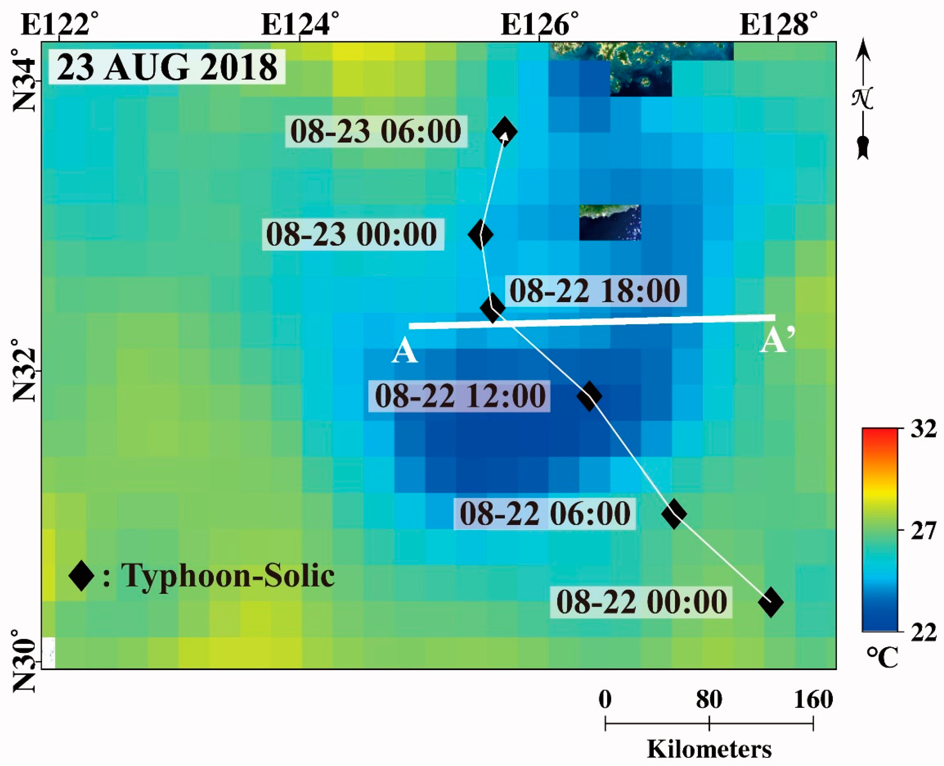
3.3. Interaction with a Typhoon

We examined the variation of the GOCI-derived SSS and CHL together with the National Oceanic and Atmospheric Administration Optimum Interpolation Sea Surface Temperature (NOAA OISST) sea surface temperature (SST) in August 2018 when Typhoon Soulik (2018) passed over the East China Sea and to the west of Jeju Island heading toward the Korean Peninsula. According to the Joint Typhoon Warning Center (JTWC) best track (Figure 7), Soulik (2018) initially formed on 15 August over the tropical western North Pacific (12.7° N, 144.4° E). On 17 August, the JTWC upgraded Soulik to a typhoon, with a peak intensity on 20 August (maximum intensity of 105 knots). When Soulik passed our study domain on 22–23 August 2018, it weakened from 90 to 65 knots.

As shown in Figure 8 and Figure 9, three weeks before the typhoon’s passage (on 1–2 August), the low salinity area in front of the Yangtze River mouth was not significant and there were no notable CHL features. The SST was relatively low over the East China Sea and the sea south of Jeju Island. However, a week before the typhoon passed (15 August), a wide low salinity plume (<26 psu) developed from the mouth of the river toward the west of Jeju Island. Further east, the salinity around the west and south coasts of Jeju Island became lower (~29 psu, yellow color in the figures) than the previous week. The increased solar heating due to atmospheric high-pressure systems over the LSW may have warmed the ocean surface [26,27], resulting in higher SSTs, as shown in Figure 8 and Figure 9.

Two days after Typhoon Soulik passed over the East China Sea (24 August), ocean cooling and decreasing salinity were obvious. The slow translation speed of Typhoon Soulik west of Jeju Island led to the formation of a cold wake that weakened the tropical cyclone [28]. The salinity change in response to a tropical cyclone can be both positive (increased salinity) or negative (decreased salinity) depending on the cyclone intensity and vertical salinity structure of the ocean [29]. In the case of Typhoon Soulik, a decreasing salinity effect was dominant along the typhoon trail and off the south coast of Jeju Island. A tropical cyclone consists of intense mesoscale convective systems leading to significant precipitation [30]. In a weak tropical cyclone, tropical cyclone-induced rain dilution may prevail in the cold wake circulation of the cyclone. A week after the typhoon passed (28 August), the ocean cooling was weaker but still persisted. An increase in the GOCI CHL due to the upwelling in the tropical cyclone was noted. According to Park et al. (2019) [28], severe sea surface cooling occurred on 23 August by the passage of Soulik. This timing of ocean physical change corresponds well with the timing of current results (i.e., between 21 and 24 August in Figure 8). We could not find any reference to examine biological variation in response to the same tropical cyclone. In general, the CHL bloom after tropical cyclone passage is several days later than the physical response [31]. In this aspect, we have confirmed the current timing of the tropical cyclone’s physical-biological response is in agreement with past studies. Therefore, we can imply that the current ocean color remote sensing of SSS and CHL in combination with the SST data was effective for detecting the critical ocean physical and biological variations in response to the tropical cyclone. However, as in Figure 8 and Figure 9d, the distribution of LSW in the study area displayed a similar pattern to that of CHL. The LSW retrieval algorithm in this study was strongly influenced by Rrs 555 (Equation (1)). The GOCI-derived CHL was based on the OC3 algorithm, in which Rrs 555 also played an important role. This should be considered when monitoring LSW from ocean color images in the area of Chl-a blooms attributed to upwelling phenomena, and to confirm the relationships with SSS and CHL, we need as many in situ measurement as possible in those area for further study.

4. Conclusions

In the coastal region south of the Korean Peninsula, LSW plumes from the Changjiang River extend to the East China Sea in the summer and affect the marine environment, causing damage to aquaculture systems. We investigated the applicability of GOCI for mapping LSW plumes in the East China Sea in the summer season when the Changjiang Diluted Water strongly influences Korean waters. The following several conclusions could be drawn from this study.

(1)

The LSW retrieval algorithm empirically developed in this study using GOCI Rrs bands 3–6 was considered reliable following a comparison with both in situ measurements and the results of two previous models used to derive SSS in the East China Sea. However, further study is needed to determine whether the algorithm is applicable to high salinity waters with samples from the study area when it is not affected by the Changjiang Diluted Water, which would enable the development of a standard algorithm for satellite-derived SSS.

(2)

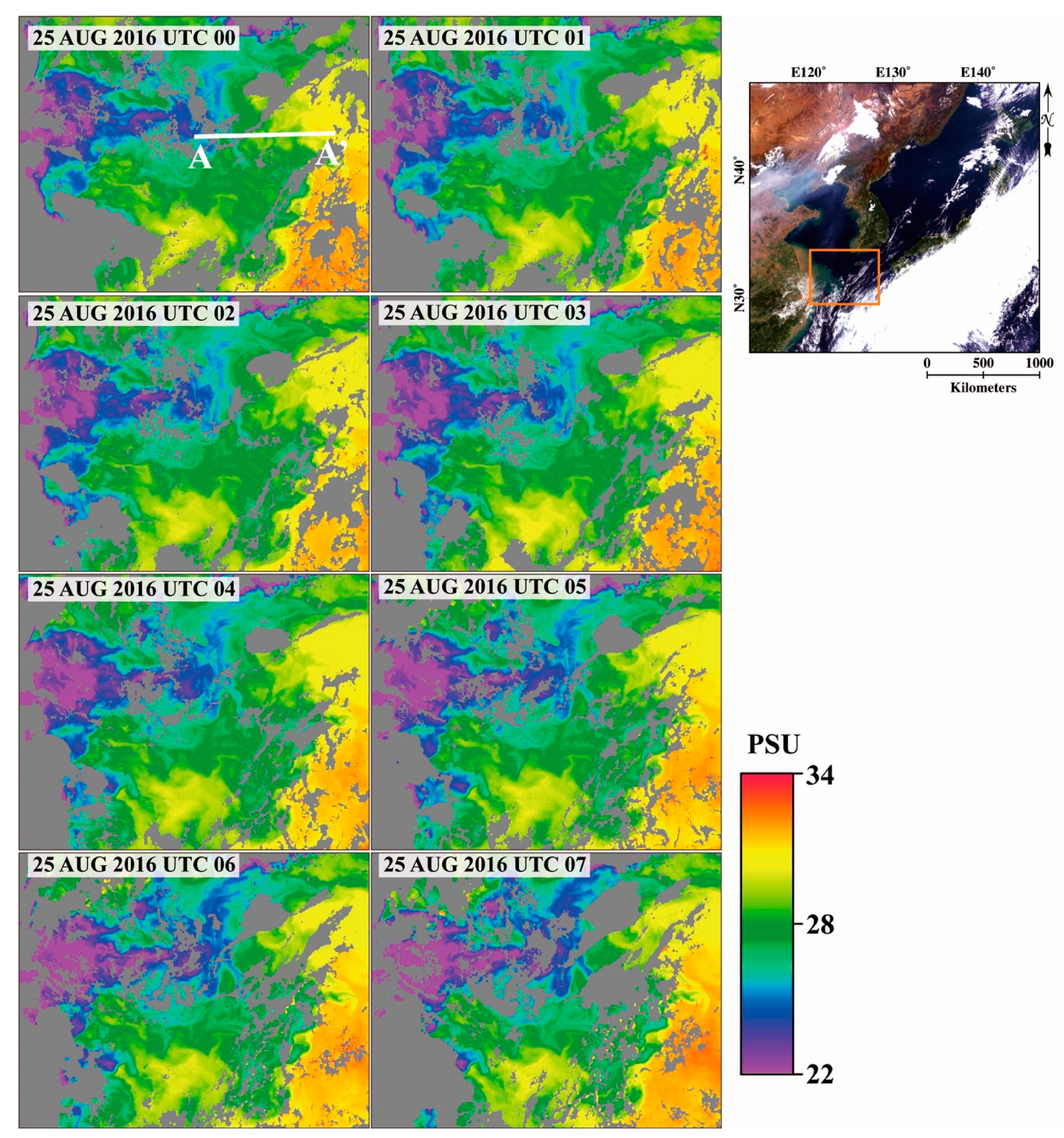
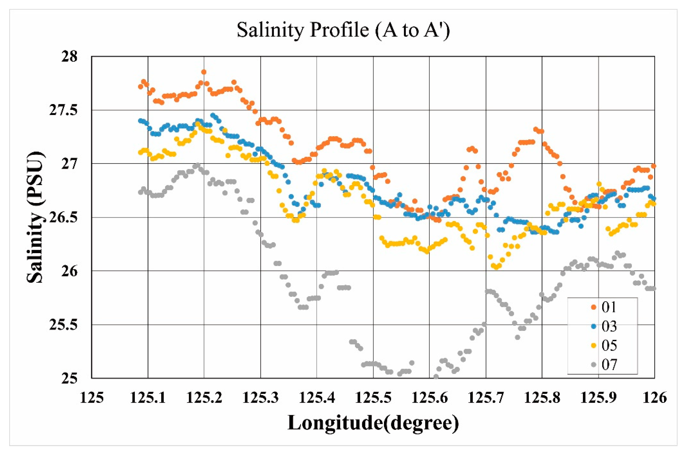
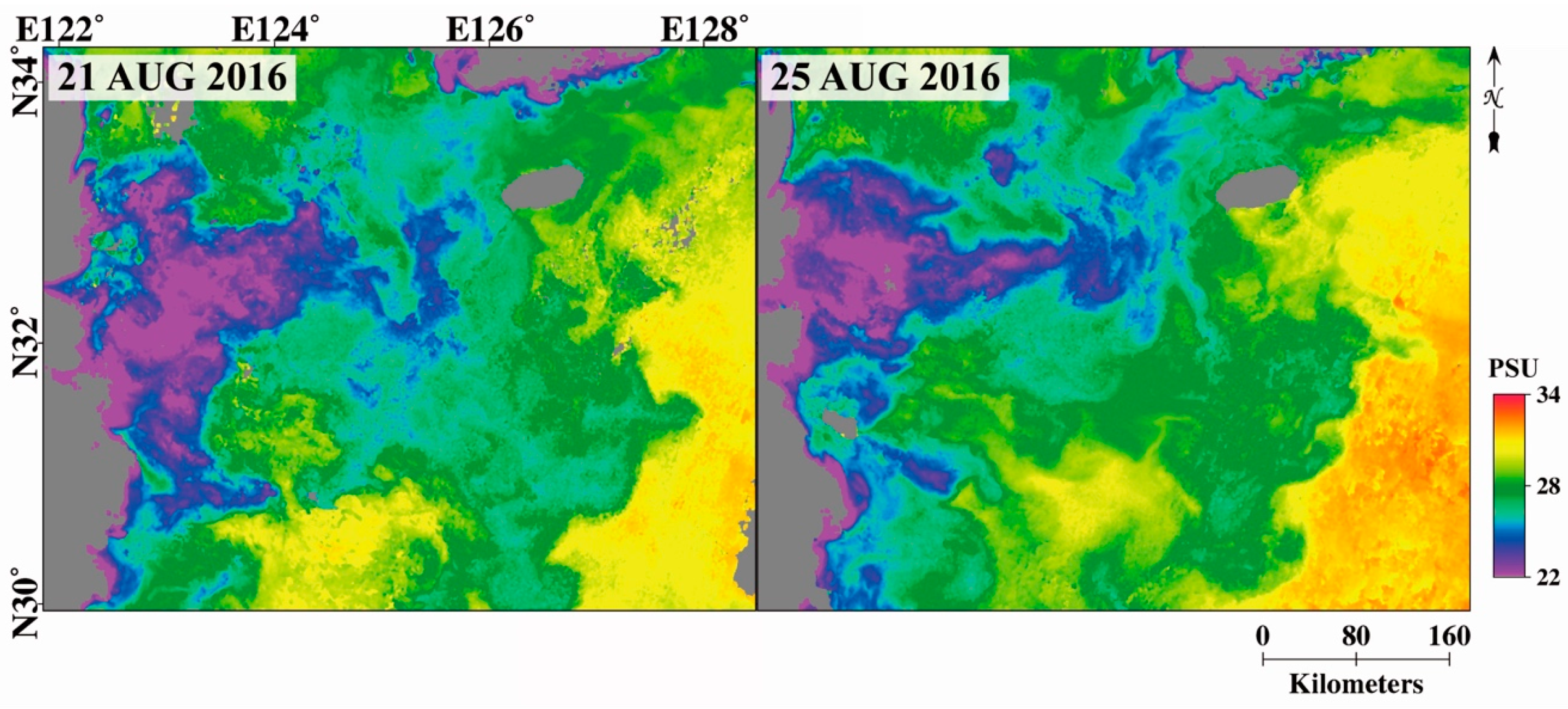
According to a time series of GOCI-derived SSS images on a diurnal and daily scale, the LSW along the east coast of China and to the north of the Changjiang River mouth extended to the northeast and influenced the southwestern part of the Korean Peninsula to the north of Jeju Island in August 2018. We found that the LSW split to the north and south near the western part of Jeju Island, extending to the Straits of Korea in the north and to the Ieodo Ocean Research Station in the south.

(3)

The variation of the satellite-derived SSS, CHL, and SST when Typhoon Soulik passed over the study area revealed that ocean cooling and decreasing salinity effects were strongly exhibited two days after the typhoon passed, and then became weaker a week after the passage. We also identified an increase in the CHL due to the upwelling in the study area resulting from the passage of Typhoon Soulik.

This study demonstrated that GOCI can be used to detect and monitor LSW plumes in the East China Sea. The empirical algorithm developed in this study for detecting LSW from GOCI data was aimed at low-salinity surface water conditions in the East China Sea. In particular, optically the study area is strongly influenced by extremely high turbidity, which makes Rrs spectra turbid water dominated [32] and the algorithm developed here site-specific. Thus, if a general algorithm to map the surface salinity in the East China Sea or other sea area using ocean color satellite sensors is needed, further studies using more in situ measurements under various marine conditions will be required. This study successfully investigated time-series variations of GOCI-derived SSS in combination with CHL and SST, and the interactions with a typhoon were determined in terms of marine physical and biological properties. To apply the SSS retrieval algorithm it is necessary to include Rrs at 555 nm, particularly in areas with Chl-a blooms.

References

1. Moon, J.H.; Hirose, N.; Yoon, J.H.; Pang, I.C. Offshore Detachment Process of the low-salinity water around Changjiang Bank in the East China Sea. J. Phys. Oceanogr. 2010, 40, 1035–1053. [Google Scholar] [CrossRef]
2. Ahn, Y.H.; Shanmugam, P.; Moon, J.E.; Ryu, J.H. Satellite remote sensing of a low-salinity water plume in the East China Sea. Ann. Geophys. 2008, 26, 2019–2035. [Google Scholar] [CrossRef] [Green Version]
3. Kim, H.C.; Yamaguchi, H.; Yoo, S.; Zhu, J.; Okamura, K.; Kiyomoto, Y.; Tanaka, K.; Kim, S.W.; Park, T.; Oh, I.; et al. Distribution of Changjiang Diluted Water detected by satellite chlorophyll-a and its interannual variation during 1998–2007. J. Oceanogr. 2009, 65, 129–135. [Google Scholar] [CrossRef]
4. Kim, D.W.; Park, Y.J.; Jeong, J.Y.; Jo, Y.H. Estimation of Hourly Sea Surface Salinity in the East China Sea Using Geostationary Ocean Color Imager Measurements. Remote Sens. 2020, 12, 755. [Google Scholar] [CrossRef] [Green Version]
5. Ciani, D.; Santoleri, R.; Liberti, G.L.; Prigent, C.; Donlon, C.; Nardelli, B.B. Copernicus Imaging Microwave Radiometer (CIMR) Benefits for the Copernicus Level 4 Sea-Surface Salinity Processing Chain. Remote Sens. 2019, 11, 1818. [Google Scholar] [CrossRef] [Green Version]
6. Droghei, R.; Nardelli, B.B.; Santoleri, R. A New Global Sea Surface Salinity and Density Dataset from Multivariate Observations (1993–2016). Front. Mar. Sci. 2018, 5, 84. [Google Scholar] [CrossRef] [Green Version]
7. Soldo, Y.; Khazaal, A.; Cabot, F.; Kerr, Y.H. An RFI Index to Quantify the Contamination of SMOS Data by Radio-Frequency Interference. IEEE J. Sel. Top. Appl. Earth Obs. Remote Sens. 2016, 9, 1577–1589. [Google Scholar] [CrossRef]
8. Mohammed, P.N.; Aksoy, M.; Piepmeier, J.R.; Johnson, J.T.; Bringer, A. SMAP L-Band Microwave Radiometer: RFI Mitigation Prelaunch Analysis and First Year On-Orbit Observations. IEEE Trans. Geosci. Remote Sens. 2016, 54, 6035–6047. [Google Scholar] [CrossRef]
9. Soldo, Y.; Le Vine, D.M.; de Matthaeis, P.; Richaume, P. L-Band RFI Detected by SMOS and Aquarius. IEEE Trans. Geosci. Remote Sens. 2017, 55, 4220–4235. [Google Scholar] [CrossRef]
10. Son, Y.B.; Gardner, W.D.; Richardson, M.J.; Ishizaka, J.; Ryu, J.H.; Kim, S.H.; Lee, S.H. Tracing offshore low-salinity plumes in the Northeastern Gulf of Mexico during the summer season by use of multispectral remote-sensing data. J. Oceanogr. 2012, 68, 743–760. [Google Scholar] [CrossRef]
11. Qing, S.; Zhang, J.; Cui, T.W.; Bao, Y.H. Retrieval of sea surface salinity with MERIS and MODIS data in the Bohai Sea. Remote Sens. Environ. 2013, 136, 117–125. [Google Scholar] [CrossRef]
12. Palacios, S.L.; Peterson, T.D.; Kudela, R.M. Development of synthetic salinity from remote sensing for the Columbia River plume. J. Geophys. Res. Oceans 2009, 114. [Google Scholar] [CrossRef] [Green Version]
13. Marghany, M.; Hashim, M. A numerical method for retrieving sea surface salinity from MODIS satellite data. Int. J. Phys. Sci. 2011, 6, 3116–3125. [Google Scholar]
14. Bai, Y.; Pan, D.L.; Cai, W.J.; He, X.Q.; Wang, D.F.; Tao, B.Y.; Zhu, Q.K. Remote sensing of salinity from satellite-derived CDOM in the Changjiang River dominated East China Sea. J. Geophys. Res. Oceans 2013, 118, 227–243. [Google Scholar] [CrossRef]
15. Ferrari, G.M.; Dowell, M.D. CDOM absorption characteristics with relation to fluorescence and salinity in coastal areas of the southern Baltic Sea. Estuar. Coast. Shelf Sci. 1998, 47, 91–105. [Google Scholar] [CrossRef]
16. Sasaki, H.; Siswanto, E.; Nishiuchi, K.; Tanaka, K.; Hasegawa, T.; Ishizaka, J. Mapping the low salinity Changjiang Diluted Water using satellite-retrieved colored dissolved organic matter (CDOM) in the East China Sea during high river flow season. Geophys. Res. Lett. 2008, 35. [Google Scholar] [CrossRef]
17. Siegel, D.A.; Maritorena, S.; Nelson, N.B.; Behrenfeld, M.J.; McClain, C.R. Colored dissolved organic matter and its influence on the satellite-based characterization of the ocean biosphere. Geophys. Res. Lett. 2005, 32. [Google Scholar] [CrossRef] [Green Version]
18. Liu, R.J.; Zhang, J.; Yao, H.Y.; Cui, T.W.; Wang, N.; Zhang, Y.; Wu, L.J.; An, J.B. Hourly changes in sea surface salinity in coastal waters recorded by Geostationary Ocean Color Imager. Estuar. Coast. Shelf Sci. 2017, 196, 227–236. [Google Scholar] [CrossRef]
19. Moh, T.; Cho, J.H.; Jung, S.K.; Kim, S.H.; Son, Y.B. Monitoring of the Changjiang River Plume in the East China Sea using a Wave Glider. J. Coast. Res. 2018, 85, 26–30. [Google Scholar] [CrossRef]
20. Choi, J.-K.; Park, Y.J.; Ahn, J.H.; Lim, H.-S.; Eom, J.; Ryu, J.-H. GOCI, the world’s first geostationary ocean color observation satellite, for the monitoring of temporal variability in coastal water turbidity. J Geophys. Res. Oceans 2012, 117. [Google Scholar] [CrossRef]
21. NIFS NIFS Serial Oceanographic Observation. 2020. Available online: http://www.nifs.go.kr/kodc/eng/eng_soo_list.kodc (accessed on 22 January 2021).
22. Moon, J.-E.; Park, Y.-J.; Ryu, J.-H.; Choi, J.-K.; Ahn, J.-H.; Min, J.-E.; Son, Y.-B.; Lee, S.-J.; Han, H.-J.; Ahn, Y.-H. Initial validation of GOCI water products against in situ data collected around Korean peninsula for 2010–2011. Ocean Sci. J. 2012, 47, 261–277. [Google Scholar] [CrossRef]
23. Choi, J.K.; Park, Y.J.; Lee, B.R.; Eom, J.; Moon, J.E.; Ryu, J.H. Application of the Geostationary Ocean Color Imager (GOCI) to mapping the temporal dynamics of coastal water turbidity. Remote Sens. Environ. 2014, 146, 24–35. [Google Scholar] [CrossRef]
24. Kim, W.; Moon, J.E.; Park, Y.J.; Ishizaka, J. Evaluation of chlorophyll retrievals from Geostationary Ocean Color Imager (GOCI) for the North-East Asian region. Remote Sens. Environ. 2016, 184, 482–495. [Google Scholar] [CrossRef]
25. Son, Y.B.; Park, G.; Ryu, J.-H.; Choi, J.-K. Algorithm for low-salinity plume in the East China Sea during the summer season using two-step empirical approach for GOCI and MODIS satellite sensors. In Proceedings of the Ocean Optics XXIV, Dubrovnik, Croatia, 7–12 October 2018; The Oceanography Society: Dubrovnik, Croatia, 2018. [Google Scholar]
26. Moon, J.H.; Kim, T.; Son, Y.B.; Hong, J.S.; Lee, J.H.; Chang, P.H.; Kim, S.K. Contribution of low-salinity water to sea surface warming of the East China Sea in the summer of 2016. Prog. Oceanogr. 2019, 175, 68–80. [Google Scholar] [CrossRef]
27. Lee, S.; Park, M.S.; Kwon, M.; Kim, Y.H.; Park, Y.G. Two major modes of East Asian marine heatwaves. Environ. Res. Lett. 2020, 15, 074008. [Google Scholar] [CrossRef]
28. Park, J.H.; Yeo, D.E.; Lee, K.; Lee, H.; Lee, S.W.; Noh, S.; Kim, S.; Shin, J.; Choi, Y.; Nam, S. Rapid Decay of Slowly Moving Typhoon Soulik (2018) due to Interactions with the Strongly Stratified Northern East China Sea. Geophys. Res. Lett. 2019, 46, 14595–14603. [Google Scholar] [CrossRef] [Green Version]
29. Reul, N.; Chapron, B.; Grodsky, S.A.; Guimbard, S.; Kudryavtsev, V.; Foltz, G.R.; Balaguru, K. Satellite Observations of the Sea Surface Salinity Response to Tropical Cyclones. Geophys. Res. Lett. 2021, 48, e2020GL091478. [Google Scholar] [CrossRef]
30. Park, M.S.; Elsberry, R.L. Latent Heating and Cooling Rates in Developing and Nondeveloping Tropical Disturbances during TCS-08: TRMM PR versus ELDORA Retrievals. J. Atmos. Sci. 2013, 70, 15–35. [Google Scholar] [CrossRef] [Green Version]
31. Subrahmanyam, B.; Rao, K.H.; Rao, N.S.; Murty, V.S.N.; Sharp, R.J. Influence of a tropical cyclone on Chlorophyll-a Concentration in the Arabian Sea. Geophys. Res. Lett. 2002, 29. [Google Scholar] [CrossRef]
32. Lee, Z.; Shang, S.L.; Lin, G.; Chen, J.; Doxaran, D. On the modeling of hyperspectral remote-sensing reflectance of high-sediment-load waters in the visible to shortwave-infrared domain. Appl. Opt. 2016, 55, 1738–1750. [Google Scholar] [CrossRef]
Figure 1. The study area and wave glider track in 2016 in the East China Sea.
Remotesensing 13 02676 g001
Figure 2. Comparison of the results obtained using the algorithm in this study with in situ SSS using 21 measurements from a test set for GOCI-derived SSS.
Remotesensing 13 02676 g002
Figure 3. Comparisons of GOCI-derived SSS in this study with the results from (a) Ahn’s model and (b) Son’s model for the image acquired at 12:30 local time on 20 August 2016. Comparison of the results obtained with in situ SSS using 21 measurements from a test set for GOCI-derived SSS using (c) the model by Ahn et al. (2008) [2] and (d) the model by Son et al. (2018) [25].
Remotesensing 13 02676 g003
Figure 4. The GOCI-derived SSS images from 09:30 (UTC 00) to 16:30 (UTC 07) on 25 August 2016 generated in this study, with the SSS profile line (AA’) also shown.
Remotesensing 13 02676 g004
Figure 5. The GOCI-derived SSS values along line AA’ in Figure 4 at 10:30, 12:30, 14:30, and 16:30 local time.
Remotesensing 13 02676 g005
Figure 6. Daily composite SSS images derived from GOCI on 21 and 25 August 2016 in this study.
Remotesensing 13 02676 g006
Figure 7. Track of Typhoon Soulik overlaid on NOAA OISST data on 23 August 2018 with the CHL, SSS, and SST profile line (AA’) also shown.
Remotesensing 13 02676 g007
Figure 8. Daily composite SSS images derived from GOCI in this study on 1, 2, 15, 21, 24, and 28 August 2018 and the corresponding GOCI-derived CHL images (the same spatial resolution with SSS observations) and NOAA OISST SST images.
Remotesensing 13 02676 g008
Figure 9. Daily SSS values along line AA’ in Figure 7 on 1, 2, 15, 21, 24, and 28 August 2018 (a) with (b) the corresponding SST values from NOAA OISST SST images and (c) GOCI-derived daily CHL values. (d) the color-coded scatter plots of SSS from (a) against CHL in(c).
Remotesensing 13 02676 g009