Abstract
Evaluating satellite ability in capturing sudden natural disasters such as heavy snowstorms is a topic of societal interest. This paper presents a rapid qualitative analysis of an intense snowfall in Madrid using data from the Global Precipitation Measurement (GPM) mission, specifically the GPM IMERG (Integrated Multi-satellitE Retrievals for GPM) Late Precipitation L3 Half Hourly 0.1° × 0.1° V06 estimates of precipitation (IMERG-Late), and Sentinel-2 imagery. The main research question addressed is the consistency of ground observations, model outputs and satellite data, a topic of major interest for an appropriate and timely societal response to severe weather episodes. Indeed, the choice of the ‘Late’ product over the IMERG ‘Final’ or other GPM datasets was motivated by the availability of data for near real-time response to the storm. Additionally, the 30-min temporal resolution of the product would in principle allow for a detailed analysis of the dynamic processes involved in the snowstorm. Using several complementary data sources, it is shown that optical remote sensing sensors (Sentinel) add value to existing ground data and that is invaluable for rapid response to severe meteorological events such as Filomena. Regarding the GPM precipitation radar, the sampling of the GPM-core satellite was insufficient to provide the IMERG algorithm with enough quality data to correctly represent the actual sequence of precipitation. Without corrections, the total precipitation differs from observations by a factor of two. The difficulties of retrieving precipitation with radiometers over snow-covered surfaces was a major factor for the mismatch. Thus, the calibrated precipitation product did not fully capture the historic storm, and neither did the IR-based element of the IMERG-Late product, which is a neural network merging of microwave and infrared data. It follows that increased temporal resolution of spaceborne microwave sensors and improved retrieval of precipitation from radiometers are critical in order to provide a complete account of these sorts of extreme, significant, short-duration cases. Otherwise, the high-quality, radar and radiometer data feeding the high temporal resolution algorithms simply slip through the grasp of the ascending and descending orbits, leaving little quality data to be interpolated into successive overpasses.
1. Introduction
Precipitation is both a key environmental parameter and a difficult meteorological field to measure. Its large spatial and temporal variability, sharp gradients and zero-skewed intensities are challenges still not fully resolved by existing measurement methods [1]. The need for good estimates, however, is evident, and extends to agriculture, industry, energy and biota studies [2,3,4,5,6,7,8].
The importance of a precise estimation of precipitation is especially acute in the case of extreme and unusual meteorological events [9,10,11]. Pinpointing the exact location of the highest precipitation rates is important, but difficult, as they can occur both in a short period of time or in regions where the rain gauge network is not as dense as near major cities and flat areas. While ground-based radars can in principle fill the gaps with high spatial and temporal resolutions, the estimation of precipitation using such instruments presents several limitations [12,13,14,15,16,17], especially over varied terrain where intervisibility and ground cluttering makes retrievals difficult. The alternative, a view from space, naturally appeared as an optimal way to estimate precipitation, especially over the oceans where ground networks are almost completely absent [18,19].
Indeed, as soon as Earth observation satellite programs began, measuring precipitation from space became a thriving research field, with many algorithms and datasets becoming available [20,21,22]. A major breakthrough, the Tropical Rainfall Measuring Mission (TRMM) satellite [23], heralded the era of precipitation radars in space in 1997. A 2014 follow-on satellite, the GPM-core observatory [24], provided continuity and improved global coverage to what is widely considered fundamental for both meteorology and climate research [25]. While several satellites are currently used to provide precipitation estimates, those of the GPM constellation are the standard and the only means to have 30-min, kilometer-resolution global estimates of precipitation on a regular basis.
The GPM-core observatory is the central part of the GPM constellation, with a suite of international radiometers to provide a complete picture of global precipitation. The Dual-frequency Precipitation Radar (DPR) and the GPM Microwave Imager (GMI) provide high-quality and the most direct estimates of precipitation available from space. The combination of other sensor completes the current picture of direct measurements of precipitation from space. The failure of CloudSat (which in any case provided only an indirect estimate of precipitation) on 27 August 2020 makes the DPR the only radar in space capable of directly observing precipitation in 2021.
January 2021 witnessed the largest snowstorm in the capital city of Spain since 1971. Thirty hours of continuous snowfall from 7 January covered Madrid in a white blanket, disrupting urban life for days. Major damage followed and casualties were reported. The event, in the midst of the COVID-19 pandemic, severely affected communications, infrastructures, buildings and vegetation. The Madrid Metropolitan area, and the Autonomous Communities of Madrid and Castilla-La Mancha were declared ‘catastrophe areas’ by the national government.
Responding to events such as storm Filomena is one of the reasons behind the development of ‘precipitation from space’ technology. The ability to precisely measure the solid phase, both in quantity and in location and timing is not only a formidable challenge but is essential to assist authorities in coping with the consequences of the storm, evaluating the damages, and predicting the effects of snowmelt in the urban environment [26,27,28]. It is also valuable for energy generation as hydropower is an important component of the energy mix in several countries. Snow falling in the mountains in winter feeds Spanish rivers in spring and fills the reservoirs and dams. Predicting the availability of the water resources in the harsh and semi-arid summer that affects most of the country is also a major need and the centerpiece of the country’s hydrological plans.
As mentioned above, the current meteorological network is clearly insufficient to provide a precise account of how much snow fell in the remote, mountain areas, so measurements from satellite precipitation algorithms is an absolute necessity. This paper aims to evaluate the potential of IMERG products to help in this task, an application considered by their developers as central to the whole GPM project [24]. While a detailed evaluation might be expected in a Ground Validation (GV) campaign, our event-study is aimed to evaluate whether or not GPM can detect the snow and if the IMERG estimates are consistent with the ground observations in the particular case of the storm in Madrid.
Over the years, many studies and reviews have specifically dealt with evaluating IMERG. These include regional analyses for Brazil, China, Pakistan, Cyprus, Korea and the Netherlands [29,30,31,32,33]. Discrepancies with observations have been described, within an overall good match with observations for large areas when data are averaged in time [34,35]. The scores for long temporal scales are indeed better than for shorter scales [36]. Research on the IMERG performances over snow covered terrain is scarce.
2. Data and Methods
MODIS (Moderate Resolution Imaging Spectroradiometer)/Terra data were used to provide a qualitative evaluation of the cloud cover. Four images were used, which were obtained through NASA’s Worldview, a tool from the Earth Observing System Data and Information System (EOSDIS). The reason for directly featuring this tool in this paper instead of reprocessing the original data is that Worldview can be readily used by managers and the general public. It is also an integral part of the GPM data dissemination strategy and a valuable instrument to rapid response to events. Using this tool, GMI daily estimates of rain rates from the 2AGPROFGMI, Level 2A Goddard Profiling algorithm were superimposed on the MODIS images to provide a qualitative indication of the GPM capability of obtaining information below the cloud cover. MODIS sensor resolutions are 500 m and 250 m (Bands 1 and 2 have a sensor resolution of 250 m, Bands 3–7 have a sensor resolution of 500 m and Bands 8–36 are 1 km. Band 1 is used to sharpen Bands 3, 4, 6 and 7). The temporal resolution is daily. The MODIS Corrected Reflectance algorithm utilizes MODIS Level 1B data (calibrated, geolocated radiances) to produce a visually acceptable, qualitative view of the planet, but which is not a standard, science-quality product. The asserted purpose of this algorithm is to provide natural-looking images by removing gross atmospheric effects, such as Rayleigh scattering, from MODIS visible bands 1–7.
Sentinel-2b data was obtained from the Copernicus Open Access Hub. Two orbits from Sentinel-2b MultiSpectral Instrument (MSI) for 3 January (S2B_MSIL2A_20210103T110349_N0214_R094) and 11 January (S2A_MSIL1C_20210111T111431_N0209_R137) were used. Their 4, 3 and 2 bands (665.0, 559.0, 492.1 nm at Full Width Half Maximum (FWHM)) were co-geolocated. Spatial resolution of those is 10 m. Original files downloaded from the Hub were processed with NCL (NCAR Command Language), Python and Fortran scripts developed at the Earth and Space Sciences Group (ESS) over the past decades. Quicklooks from the Sentinel-3 Sea and Land Surface Temperature Radiometer (SLSTR) were also retrieved from https://www.sentinel-hub.com/, accessed on 25 May 2021.
Weather analyses from the European Centre for Medium-Range Weather Forecasts (ECMWF) were used to depict the atmospheric situation and explain the evolution of Storm Filomena. Original grib files were processed at UCLM using ncl and Python scripts developed at the Earth and Space Sciences Group (ESS).
Official reports from the Agencia Estatal de Meteorología (AEMET) [37] were used as the source of reference for observational ground data. As the episode consisted in heavy wet snow with little wind, gauge-recorded precipitation can be trusted. Snow-depth measurements are official data from the observatory and found to be consistent with gauge estimates. In any case, these data are the official estimates and there is no reason not to take them as a valid reference. The recorded amounts are unprecedented in modern times in Madrid and resulted in the central and southeastern part of the country being severely disrupted for days. It has to be noted that such severe snowstorms are uncommon in Central Spain.
IMERG (Integrated Multi-satellitE Retrievals for GPM) estimates for this paper were obtained from the Precipitation Processing System (PPS). The IMERG algorithm is fully and precisely described by Huffman et al. [38]. It would be futile to rephrase the wording of a technical document written by the actual developers of the algorithm, so in what follows we merely quote verbatim those parts relevant for this paper. The reader is directed to the original source for the additional details and a full description of the products.
Thus, as stated in the Algorithm Theoretical Basis Document Version 6 (ATDB), the aim of the product is to provide a spatial and temporally continuous estimate of precipitation for the whole globe. The algorithm is intended to intercalibrate, merge, and interpolate all satellite microwave precipitation estimates, together with microwave-calibrated infrared (IR) satellite estimates, precipitation gauge analyses and potentially other precipitation estimators at fine time and space scales for the TRMM and GPM eras over the entire globe [38].
Intercalibrated microwave precipitation estimates from GPM and all of the partner sensors are merged to create Level 3 data sets containing the best observational data available in each half hour. All of the input data sets are gridded from their native Level 2 swath data to the IMERG 0.1° × 0.1° Level 3 global grid on the IMERG half-hourly interval (namely the first and second half hour for each UTC hour) [38].
IMERG infrared precipitation field uses the ‘Precipitation Estimation from the Remotely Sensed Information using the Artificial Neural Networks – Cloud Classification System’ (PERSIANN-CCS, [39]), which is a neural network-based algorithm fusing the infrared and passive microwave radiances in a non-trivial way. The network was trained to CMORPH [40,41].
In particular, following the ATDB the IMERG IR product is derived as follows. First, the 60 °N-60 °S domain in segmented into 24 subregions. Then, for each subregion the number of watersheds is calculated and a ‘precipitation index’ is computed for each grid box. Finally, as the PERSIANN-CCS estimate is trained to CMORPH, a regional PERSIANN-CCS/PMW correction table based on monthly accumulated coincident histograms is applied. IR is exclusively used for precipitation estimates when the PMW has less skill due to excessive propagation (see below), or where the NOAA’s ‘Autosnow product’ indicates cold surface and therefore the PMW estimates lost their integrity [38].
Information on the snow cover is derived from the Advanced Very High Resolution Radiometer (AVHRR) onboard MetOp satellites, imagers onboard Geostationary Operational Environmental Satellites (GOES) East and West, Spinning Enhanced Visible and Infrared Imager (SEVIRI) onboard Meteosat second Generation (MSG), and Special Sensor Microwave Imager/Sounder (SSMIS) onboard Defense Meteorological Satellite Program (DMSP) satellites. Ice cover is derived from the MetOp AVHRR and DMSP SSMIS data. Both snow and ice are identified in satellite images using threshold-based decision tree image classification algorithms. Information on snow and ice cover derived from observations in the visible/infrared and the microwave bands is combined to generate continuous (gap-free) maps on a daily basis. The main output product of the system is a daily global snow and ice cover map generated on a 0.04° lat/lon grid (Plate Carree), which is about 4 × 4 km at the Equator [38].
Here we have used three IMERG fields: The High Quality (HQ) field, the Precipitation Calibrated (PC) field and the Infrared-based (IR) field. The HQ field is the merged microwave-only precipitation estimate from the GPM-core and the passive microwave (PMW) radiometers of the constellation, including: the Advanced Microwave Scanning Radiometer-2 (AMSR-2) on JAXA’s Global Change Observation Mission-Water 1 (GCOM-W1) satellite; the Advanced Technology Microwave Sounder (ATMS) instruments on the Suomi National Polar-orbiting Partnership (SNPP) and NOAA20 satellites; the multi-channel microwave humidity sounder Sondeur Atmosphérique du Profil d’Humidité Intertropicale par Radiométrie (SAPHIR) on the Megha-Tropiques satellite; the Microwave Humidity Sounder (MHS) instrument on the NOAA19 satellite; the MHS instruments on the MetOp series of satellites (EUMETSAT); and the SSMIS instruments on DMSP satellites.
The Calibrated Precipitation (CP) product fills the gaps between HQ data by driving and adjusting them through motion vectors derived from model water vapor estimates. HQ data is thus propagated. In a sense, the CP is the standard IMERG field (i.e., what is widely considered ‘the IMERG precipitation estimate’). The sampling is 30 min. There are three IMERG runs: Early, Late and Final. Thus, the system is run several times for each observation time, first giving a quick estimate (IMERG Early Run, IMERG-E) and successively providing better estimates as more data arrive (IMERG Late Run, IMERG-L). The final step uses monthly gauge data to create research-level products (IMERG Final Run, IMERG-F) [38].
The IMERG-L is computed about 14 h after observation time, so sometimes a microwave overpass is not delivered in time for the Late Run, but subsequently comes in and can be used in the IMERG-F. This would affect both the half hour in which the overpass occurs, and (potentially) morphed values in nearby half hours [38]. The main difference in terms of processing between the IMERG-E and IMERG-L is that Early only has forward propagation (which amounts to extrapolation forward in time), while the Late has both forward and backward propagation (allowing interpolation). As well, the additional latency allows lagging data transmissions to make it into the Late run, even if they were not available for the Early [38].
There are two possible factors which contribute to differences in the IMERG Late Run and Final Run datasets: The Late Run uses a climatological adjustment that incorporates gauge data. The Final run uses a month-to-month adjustment to the monthly Final Run product, which combines the multi-satellite data for the month with GPCC (Global Precipitation Climatology Centre) gauges. Its influence in each half hour is a ratio multiplier that is fixed for the month, but spatially varying [38].
As mentioned above, here we have used the IMERG-L. Its latency (about half a day) is suitable for rapid response to events such as Filomena. Another reason to use IMERG-L is that IMERG-F is gauge-calibrated, so no proper comparison with the ground observation can be made in our case. The estimates from AEMET’S Retiro station are actually incorporated (with five other stations) to the IMERG-F via the GPCC. To calculate the accumulations and to avoid interpolating missing values, we simply added the individual estimates.
3. Results
Storm Filomena hit continental Spain from the 7th to the 12th of January 2021. It has been considered a historic meteorological event by AEMET as it resulted in a highly unusual half meter of snow in Madrid city. The snowstorm on the 8th and 9th ranked as the largest in Madrid since 1971. On that occasion, also about 30 cm of snow felt over the city.
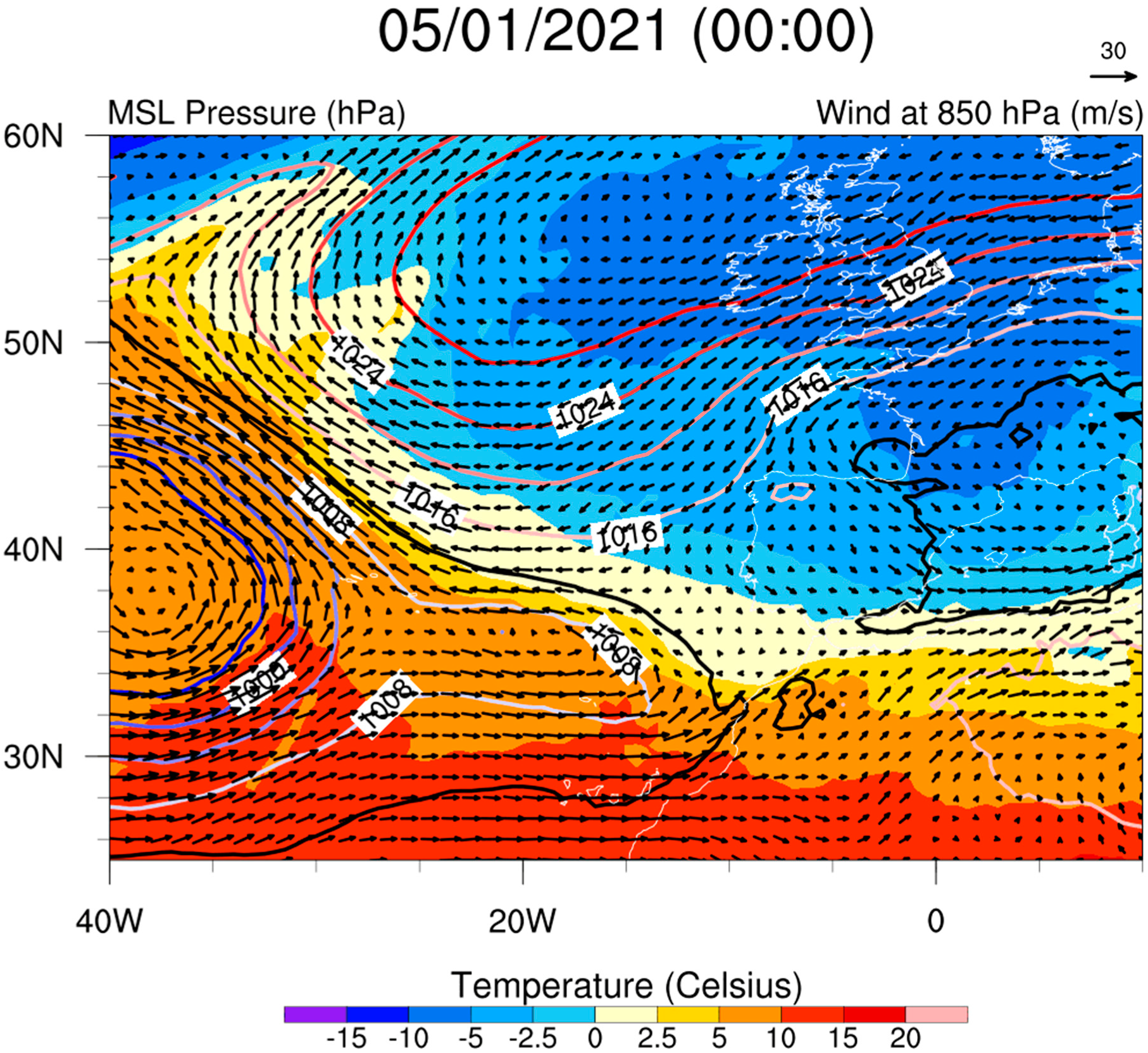
The inception of Filomena was as a perturbation in the US on 1 January 2021, and was first followed by the usual extratropical storms in the Northern hemisphere ‘hanging’ from the jet stream. However, on 6 January the storm suddenly moved south, heading to the Canary Islands as a consequence of strong high pressure stationed in high latitudes that deflected the flow (Figure 1). This excursion of the perturbation to subtropical latitudes resulted in a profound moistening of the air. Subsequent advection of the now warm, moist perturbation to the mid latitudes of the Iberian Peninsula, where cold, polar air was flowing, resulted in a slantwise clash of two different air masses with an occluded front crossing Spain from southwest to northeast.
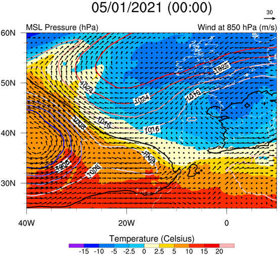
Figure 1.
ECMWF analysis, depicting the evolution of the surface pressure, the 850 hPa temperature and the 850 hPa wind from Jan 5th to 10th. Original raw data (grib files) from the ECMWF. Processing and graphics done at UCLM. [The sequence of events can be found in animated format. If reading a static version of this text please see the animated figure in the supplementary information Figure S1].
The dynamics of Filomena are a classic, yet eminent, example of the processes yielding precipitation in mid latitudes. Such encounters have been atypical in Spain both in occurrence and in magnitude: the dominant circulation from the west brings most of the precipitation in fall and spring to the northern part of the country, and otherwise moderate winter snow in Madrid usually comes from the north (polar intrusions of cold air from the continent), and seldom from the south.
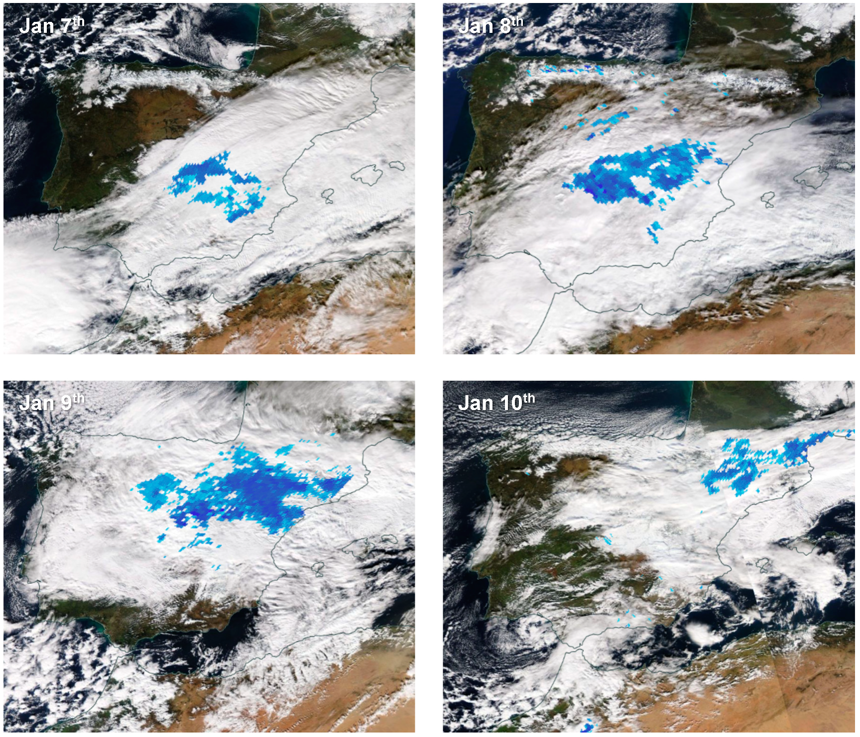
Figure 2 shows the situation on 7 January. MODIS images show the resulting cloud cover, and the GPM data (2AGPROFGMI) over the clouds identify the occurrence of solid precipitation. The data is not exactly synchronous but that is unimportant as the figure is aimed to illustrate GPM ability to retrieve information below the cloud cover.

Figure 2.
Terra/MODIS (1/4/3, ‘true color’ combination) imagery with GPM (GMI) snow detection (blues) for the 7th to the 10th of January 2021. The GPM product is the 2AGPROFGMI (‘Level 2A Goddard Profiling algorithm’ or ‘GPM_2AGPROFGPMGMI’). 2AGPROFGMI has a daily resolution. Areas in blue are those where the 2AGPROFGMI has detected snow.
For more than 30 h, snow fell continuously on the city, leaving more than 50 cm of accumulated snow. No assumptions are made over the quality of the estimates or the snowfall ratios used to convert to liquid water. It should be noted, however, that there is a large uncertainty in the reference data that impedes a pure quantitative analysis. In general, in rain gauges there is a documented underestimation of solid phased precipitation if there is not a fence installed to reduce wind effects [28]. However, the issue does not affect the results of this paper as the tens of centimeters of snow over most of the city were evidence enough of a large, unprecedented snowstorm.
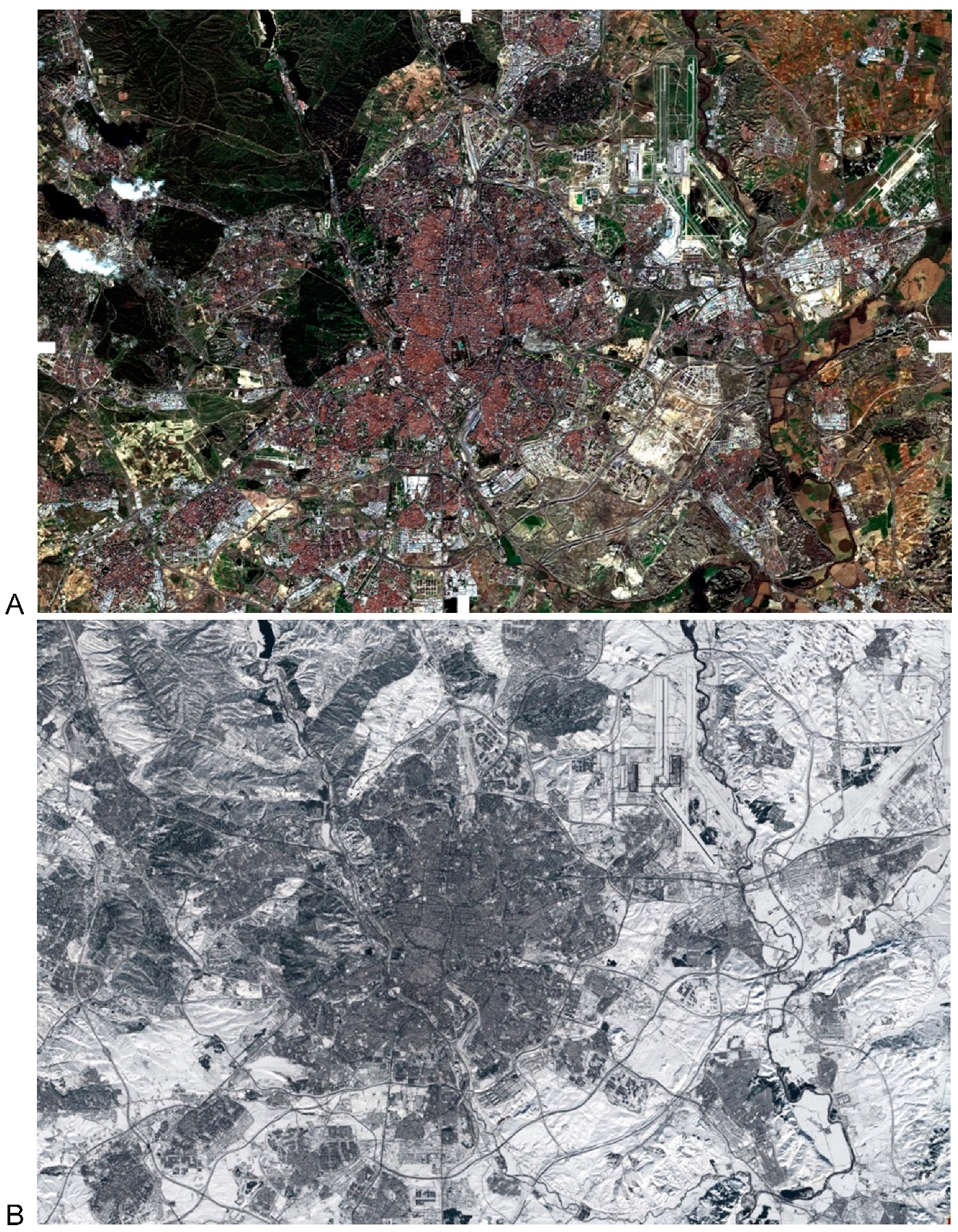
There is no doubt that Retiro park, in the very middle of the urban area (Figure 3, the central pond of the park is easily identifiable as a blue area) got 52.9 cm, while at the international airport (vertical airstrips at the top-right of Figure 3), the amount was 38.2 cm. The snow cover extended well into the South of the Madrid region (Figure 4).

Figure 3.
Sentinel 2B MSI views of Madrid city. (A): 13:07Z, 3 January; (B): 13:24Z 11 January. Both images are the ‘true color’, 4/3/2 bands combinations. White indents in the margins in the top image pinpoint the pond at Retiro Park. Raw data from the Copernicus service; processing and graphics done at UCLM.
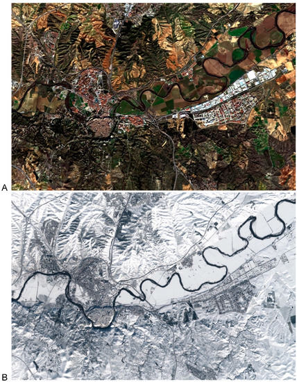
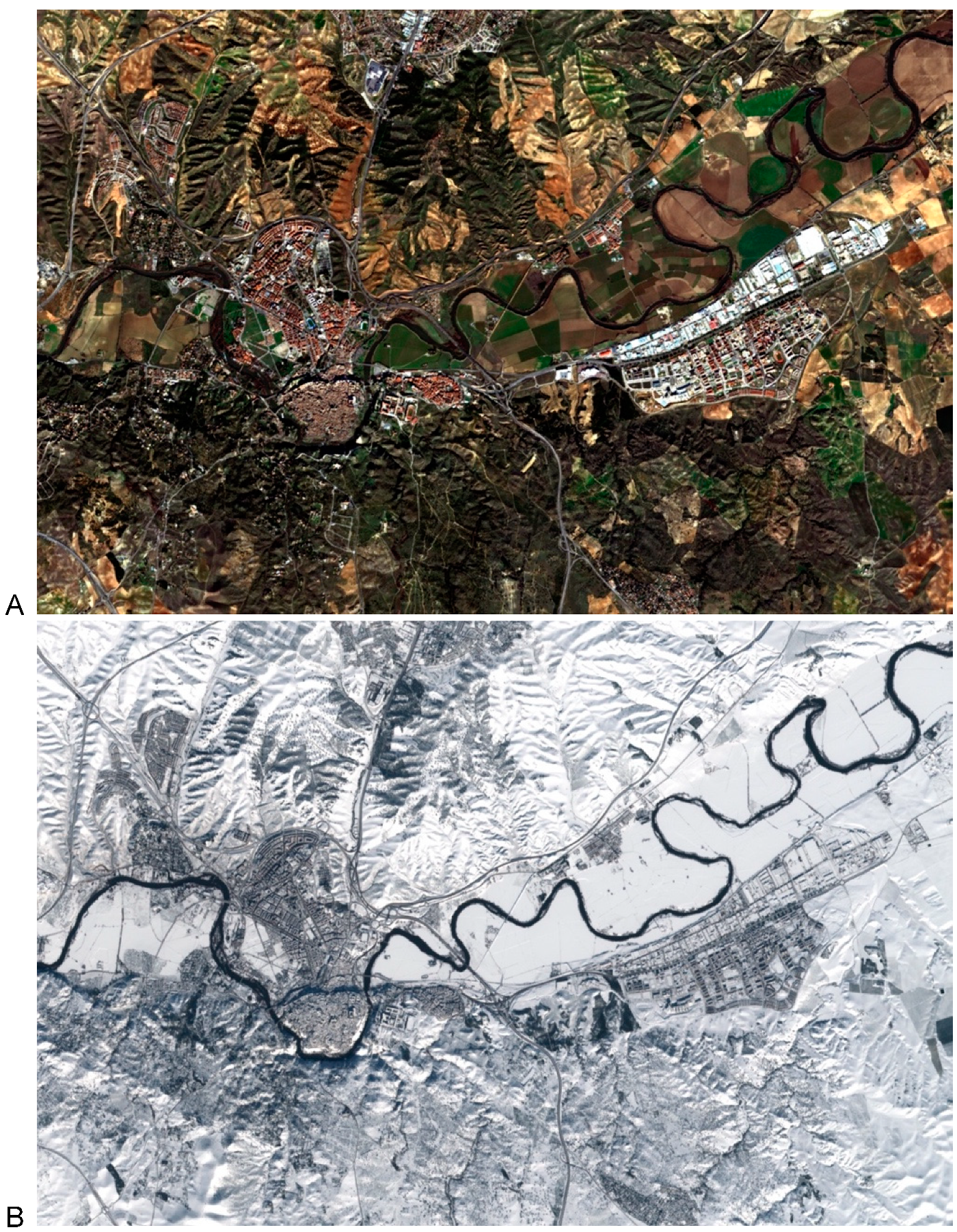
Figure 4.
Sentinel 2B MSI views of Toledo city (in Castilla-La Mancha region). (A): 13:07Z, 3 January; (B): 13:24Z 11 January. Both images are the ‘true color’, 4/3/2 bands combination.
The IMERG view of Filomena depends on the accumulation period considered. The water-equivalent total amounts for Madrid are close to the observations up to a factor of two: from 7 January 07:00 Z to 12 January 07:00 Z, the Madrid observatory in Retiro park measured 52.9 mm. The IMERG HQ field estimated 24.2 mm, the IR field read 15.3 and the Precipitation Calibrated field showed 26.1 mm.
4. Discussion
What is the explanation for the mismatch between IMERG and observations? Inspection of the animated sequence in Figure 5 shows that the HQ data were too sparse in time. Figure 2 shows that, when available, GMI data (the level 2A Goddard Profiling algorithm GPROF) provided unparalleled observational capabilities of what was happening below the cloud cover. Snow is indeed identified, something which it is impossible to sense at IR frequencies. However, HQ observations are infrequent at the latitude of Madrid. The HQ field in Figure 5 was missing for long periods.
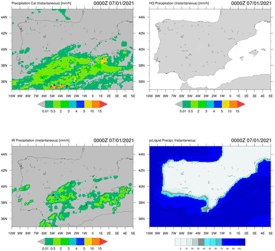
Figure 5.
The evolution of the precipitation over Spain every 30 min for 7th January to 9th, as described by three fields of the IMERG-L algorithm (Calibrated, HQ and IR), plus the estimated probability of liquid precipitation (included in the IMERG-L files). The spatial resolution of the estimates is 0.1° (about 10 km at the latitude of Madrid). The top square in the middle corresponds to the Madrid area (Figure 3), the lower is the Toledo area (Figure 4). Raw data were obtained from the Precipitation Processing System (PPS); processing and graphics were done at UCLM using Fortran programs and NCL scripts. [The sequence of events can be found in animated format. If reading a static version of this text, please see the animated figure in the supplementary information Figure S5].
Figure 6A shows the gaps in the Madrid series. This sampling affects further propagation of the estimates, which are advected over integral water vapor trajectories. The temporal interval between the HQ estimates is sometimes quite long (e.g., for Jan 9th midnight, Figure 6A), and the IR estimate then has to be infused into the calibrated product. Yet, the IR field, derived through the PERSIANN-CCS neural network multidimensional regression, is not sufficiently sensitive to discern snow which is not coming from deep convection (and thus high cloud tops) but from a forced ascent of the warm air mass.
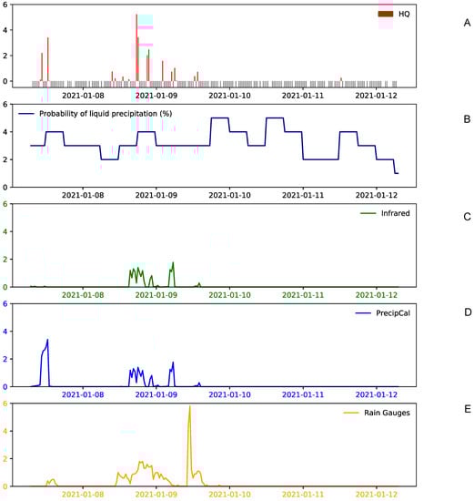
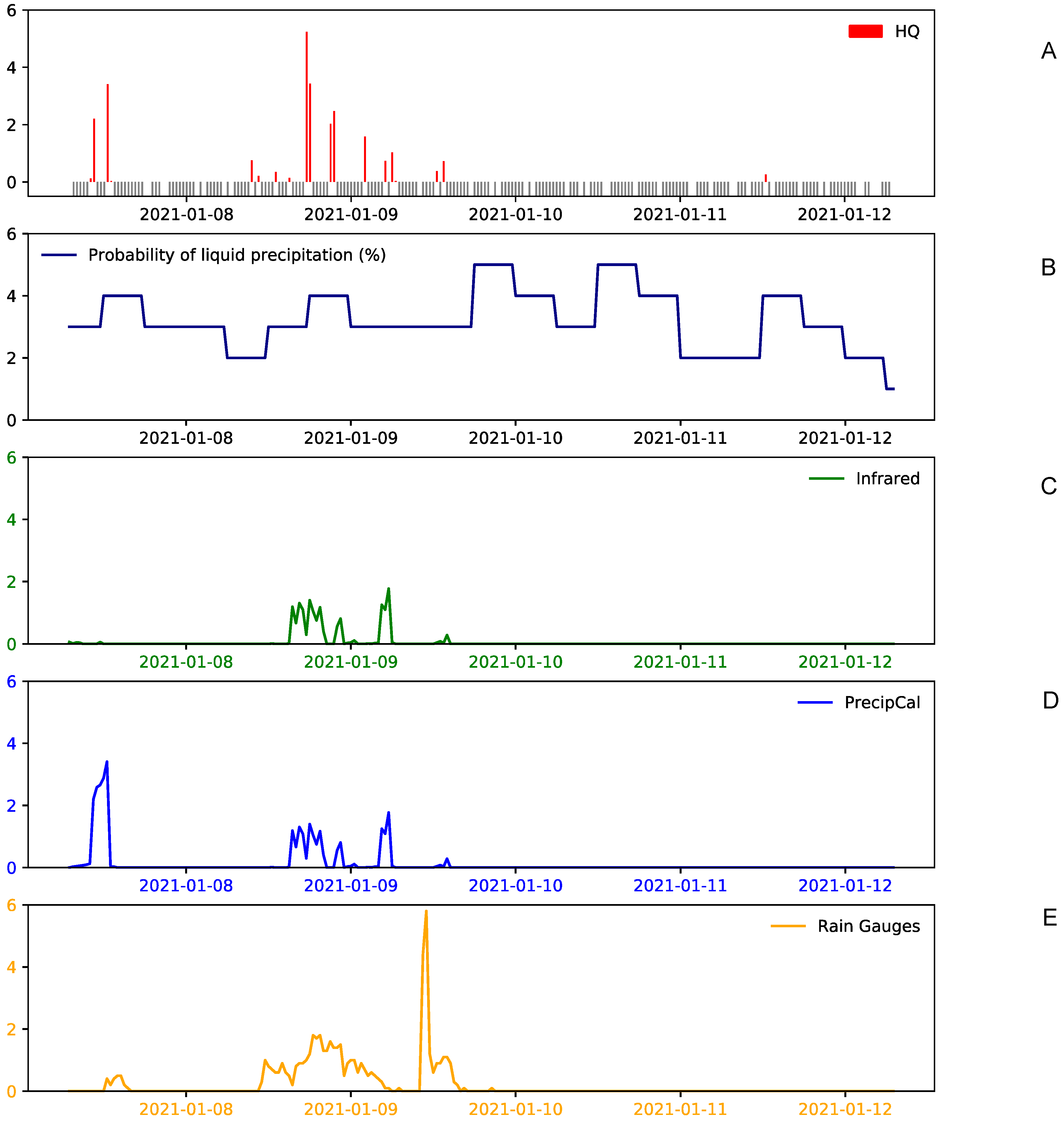
Figure 6.
The evolution of the precipitation associated with storm Filomena every 30 min at the Retiro Park meteorological station, Madrid (Latitude: 40°24′43″ N, Longitude: 3°40′41″ W, Altitude 667 m, panel E) and the estimations by the IMERG-Late algorithm (High-Quality (HQ), Infrared and Calibrate Precipitation (PrecipCal) products). Units are mm/hr. High-quality data (A) is discontinuous, so bar graphs are used. Grey marks in A indicate no data. Original rain gauge data from AEMET. IMERG data were processed using UCLM’s Fortran programs and NCL and Python scripts from the original Level-2 PPS files (B–E).
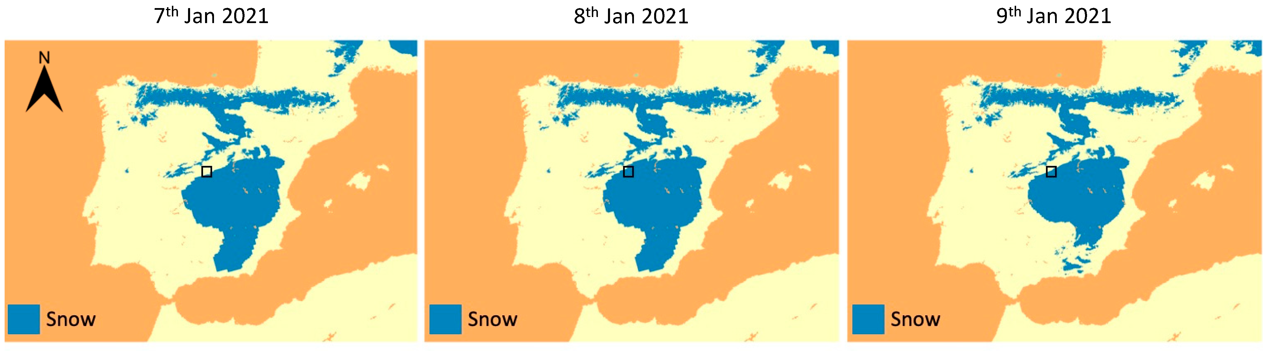
A second explanation, sampling issues aside, is that IR precipitation is used in place of observed or propagated PMW, not only when the time span between HQ data exceeds a threshold but also whenever there is a cold surface, which is identified through the ‘Autosnow’ product. This product is used at two stages in IMERG: (1) mask snow/ice surface in the computation of the Kalman statistics, and (2) mask the output IMERG precipitation estimates. IMERG uses all microwave estimates in the merge and propagation steps to allow for eventual global coverage when the microwave estimates have integrity over cold surfaces [38]. If that is not the case, the application of the NOAA/NESDIS Interactive Multisensor Snow and Ice Mapping System (IMS) information (Figure 7) results in the IR precipitation data being used and, therefore the estimates are biased lower and are less related to PMW information. While the propagation of the PMW with the IR should in general mitigate this issue, the occurrence of precipitation is still dictated by the IR, which may be low or zero [38]. The IMS product is consistent with Sentinel-3 quicklook (Figure 8).
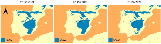
Figure 7.
4 km resolution snow coverage estimate produced by the NOAA/NESDIS Interactive Multisensor Snow and Ice Mapping System (IMS) for the 7th, 8th and 9th of January 2021. Madrid area is boxed. Raw data from NOAA/NESDIS processed using UCLM’s Fortran programs and NCL scripts.
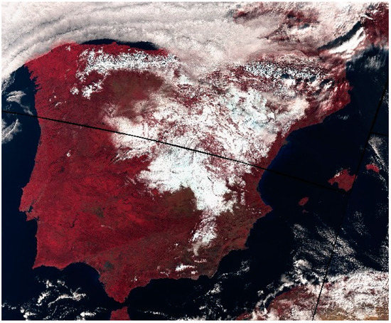
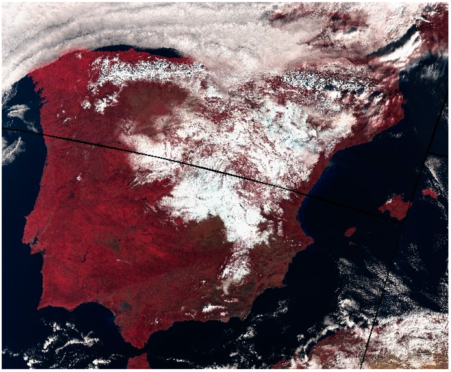
Figure 8.
Quicklook of Sentinel-3 Sea and Land Surface Temperature Radiometer (SLSTR) S3/S2/S1 band combination for 12/01/2021. Image retrieved from https://www.sentinel-hub.com/, 25 May 2021.
Figure 6 allows to quantitatively compare the evolution of the precipitation associated with storm Filomena every 30 min at the Retiro Park meteorological station, Madrid (Latitude: 40°24′43″ N, Longitude: 3°40′41″ W, Altitude 667 m) and the estimations by the IMERG-Late algorithm (High-Quality (HQ), Infrared and Calibrate Precipitation (PrecipCal) products). In the Madrid area, the Autosnow was active from Jan 8th so there is little difference between the Infrared and the PreciCal estimates from 8 January onwards (Figure 6C,D). Notwithstanding that the gauge data (E) may be underestimating the amounts, there is still a noticeable difference between the high-quality (A), the infrared (C) and the calibrated (D) products. The large number of missing slots in the high-quality series (grey marks in Figure 6A) and the low probability of liquid precipitation (B) results in inconsistencies with the Sentinel-2B imagery (Figure 3) and in situ observations: the continuous precipitation starting in the morning of January 8th, which is depicted in Figure 6E and resulted in snow covering large areas of the territory (Figure 8), appears broken in the satellite series.
Note that the largest peak in the rain gauges series in Figure 8E is due to sudden melting of accumulated snow: the largest bar in the HQ product seems to indicate that the peak of the storm in Madrid happened at that moment. Even when rain gauges are heated, large snow rates can pile up a massive amount of snow in the gauge, and it is only a few hours later that an otherwise bogus maximum features in the rain gauges series. Aggregated, one-day accumulations may palliate this particular effect in this case. The differences in the precipitation sequence are apparent: there are long periods of time when the continuous 30-h snowfall was not sensed by the continuous fields (precipitation Cal and IR precipitation), effectively meaning that the IMERG saw no precipitation at that particular moment. Such observation illustrates the many nuances when dealing with precipitation estimation, and the need of continuous filtering of the rain gauge series in snow episodes such as the one studied here.
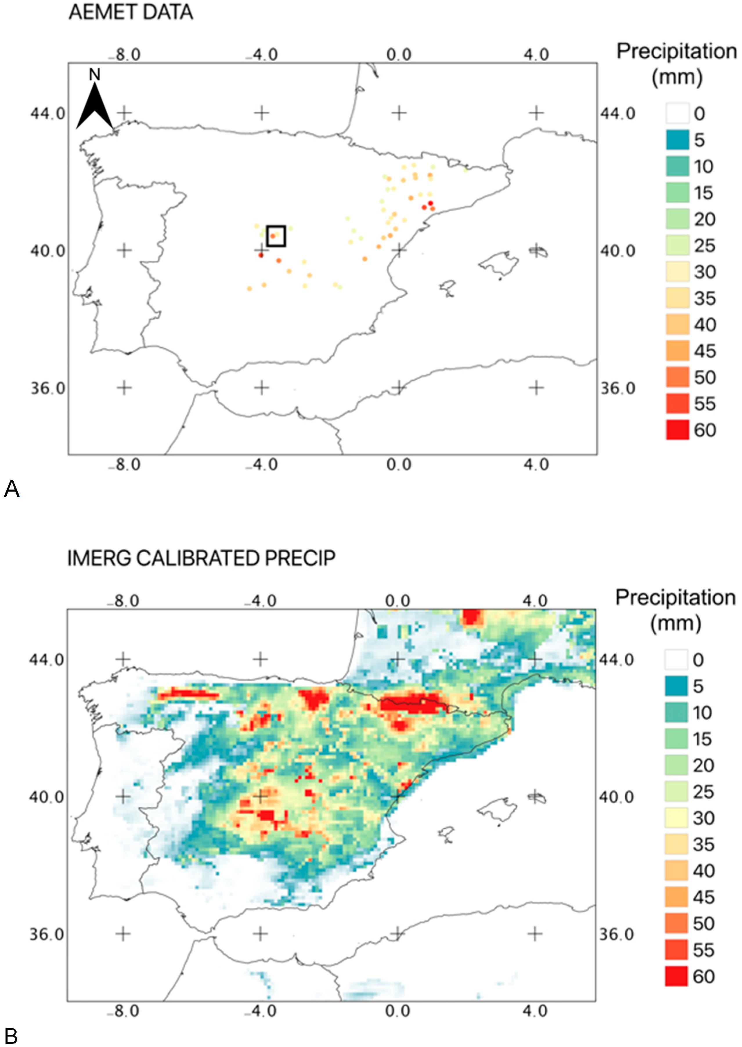
Indeed, the IMERG sequence differs from the AEMET observations. The accumulations (Figure 9) also show noticeable differences. Beyond the admittedly scarce ground quantitative data, the effects of such a conspicuous snowstorm are easy to identify and there is no doubt, not least because of direct observation on the field, that more than 30 cm of snow covered the regions under the catastrophe zone.
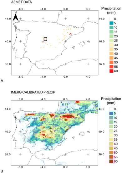
Figure 9.
(A) Official AEMET data of the precipitation amount in Spain from 7 January 07:00 Z to 12 January 07:00 Z (Table in [37]; Madrid area is indicated by a square), and (B) IMERG PrecipCal estimates for the same period, assuming snow where the probability of liquid precipitation is lower than 70% (to ease comparisons, the two plots can be found superimposed in animated format as supplementary information Figure S9).
To summarize, the evolution of the largest, historical snowstorm in Madrid in recent times is not well represented in the IMERG dataset. While the Final IMERG product, once rain gauge stations are used to recalibrate the data, might improve the 30-min estimates in areas with poor gauge coverage such as the mountains, the fact is that satellite-only estimates seem unable to capture the event and only the accumulated values compare favorably with a qualitative assessment of the episode. Such a shortcoming in the precipitation sequence is indeed irrelevant to the overall value of the algorithm and the good performances shown for accumulated amounts over the country. What is important is that the analysis of the potential causes of IMERG missing Filomena can help to improve future versions and to identify needs in instrumentation.
5. Conclusions
This paper has presented a qualitative analysis of the GPM view of the Filomena storm of 2021 using the GPM IMERG Late Precipitation L3 Half Hourly 0.1° × 0.1° V06 estimates of precipitation and also Sentinel-2b and Terra/MODIS imagery. It has been shown that the optical sensors add value to existing ground-based data, which is invaluable for rapid response to severe meteorological events such as Filomena. A combination of insufficient overpasses and cold surface affecting the retrieval of precipitation through PMW frequencies hinders IMERG reproducing the sequence of precipitation as described by the observations. Thus, the calibrated precipitation product did not fully capture the historical storm, as neither did the IR-based product of the IMERG-L, which is a neural network merging of microwave and infrared data. The total accumulations (with and without morphing of the HQ fields) are different from ground-based observations by a factor of two.
It follows that increased temporal resolution of the radiometers and radars might be a must in order to provide a complete account of these sorts of extreme, significant, short-duration cases. Otherwise, the high-quality microwave data informing the high temporal resolution algorithms simply slip through the grasp of the ascending and descending orbits, leaving little to be interpolated into successive overpasses. However, PMW retrievals are also greatly affected by the snow cover. In those cases, the IMERG has to rely on infrared data, which is not an optimal solution in terms of the directness of the estimates. Seeking solutions to evaluate the impact of events such as Filomena over densely populated areas is important and worth to be pursued, so both problems should be addressed in future research. Indeed, more investigations and a more quantitative analysis for such events are needed. This paper is focused on a single episode and with an interest in the prompt response to the event.
There is potential in the ground infrastructure to improve the response of the country to extreme events. Notwithstanding that IMERG data is also unreliable for this episode, the official data for the Filomena storm from AEMET are not accurate enough for most real-time applications. While there is no question about Madrid receiving more than 30 cm of snow during Filomena, the current raingauge network seems unprepared to cope with similar events. The issues with heated nivometers, which stop working when the cold is very intense, freezing the measuring mechanism and making the heating ineffective because it is out of the operating range, hinder research and limit the response to extreme weather events. Additional types of snowfall gauges (weight, wave systems, etc.) should be considered in the near future to enhance the observational capabilities of snow storms. Upgrading to the latest generation of rain gauges and polarimetric radars would increase current observational capabilities and help with emergencies. Therein, more investment in the existing meteorological network of Spain seems also a must.
It also seems important to prepare the observation systems for the advent of similar episodes to Filomena, and to build a denser constellation of orbital radar and radiometers that can help society better respond to more frequent severe weather events. Indeed, frequent phenomena such as Filomena can be considered a consequence of ongoing global change [42,43]. While the connection ‘more global warming, more frequent severe snowstorms’ often puzzles the general public, the rationale is simple, as greater climate variability is indeed expected in a warmer climate in which the water cycle has speeded up, albeit in the mid latitudes the role of the Artic amplification may also be relevant and requires further scrutiny [44].
Supplementary Materials
The following are available online at https://www.mdpi.com/article/10.3390/rs13142702/s1, Figures S1, S5 and S9.
Author Contributions
F.J.T. led the research and drafter the manuscript. A.V.-P., A.N., K.K., G.L. and F.J.T. contributed to analysis and manuscript writing. F.J.T. led the project. A.M., R.M., E.G.-O., J.L.S. contributed to analyses. All authors have read and agreed to the published version of the manuscript.
Funding
Funding from projects PID2019-108470RB-C21, PID2019-108470RB-C22 (Agencia Estatal de Investigación) and LE240P18 (Consejería de Educación, Junta de Castilla y León) is gratefully acknowledged. K.K. and G.L. greatly appreciate the support from the Korea Environmental Industry and Technology Institute (KEITI) of the Korea Ministry of Environment (MOE) as “Advanced Water Management Research Program” (79615).
Conflicts of Interest
The authors declare no conflict of interest.
References
- Michaelides, S.; Levizzani, V.; Anagnostou, E.; Bauer, P.; Kasparis, T.; Lane, J.E. Precipitation: Measurement, Remote Sensing, Climatology and Modeling. Atmos. Res. 2009, 94, 512–533. [Google Scholar] [CrossRef]
- Peng, F.; Zhao, S.; Chen, C.; Cong, D.; Wang, Y.; Ouyang, H. Evaluation and Comparison of the Precipitation Detection Ability of Multiple Satellite Products in a Typical Agriculture Area of China. Atmos. Res. 2020, 236, 104814. [Google Scholar] [CrossRef]
- West, H.; Quinn, N.; Horswell, M. Remote Sensing for Drought Monitoring & Impact Assessment: Progress, Past Challenges and Future Opportunities. Remote Sens. Environ. 2019, 232, 111291. [Google Scholar]
- Bartlam-Brooks, H.L.A.; Beck, P.S.A.; Bohrer, G.; Harris, S. In Search of Greener Pastures: Using Satellite Images to Predict the Effects of Environmental Change on Zebra Migration. J. Geophys. Res. Biogeosci. 2013, 118, 1427–1437. [Google Scholar] [CrossRef] [Green Version]
- Rumiano, F.; Wielgus, E.; Miguel, E.; Chamaillé-Jammes, S.; Valls-Fox, H.; Cornélis, D.; Garine-Wichatitsky, M.D.; Fritz, H.; Caron, A.; Tran, A. Remote Sensing of Environmental Drivers Influencing the Movement Ecology of Sympatric Wild and Domestic Ungulates in Semi-Arid Savannas, a Review. Remote Sens. 2020, 12, 3218. [Google Scholar] [CrossRef]
- Toté, C.; Patricio, D.; Boogaard, H.; Van der Wijngaart, R.; Tarnavsky, E.; Funk, C. Evaluation of Satellite Rainfall Estimates for Drought and Flood Monitoring in Mozambique. Remote Sens. 2015, 7, 1758–1776. [Google Scholar] [CrossRef] [Green Version]
- Bertini, C.; Buonora, L.; Ridolfi, E.; Russo, F.; Napolitano, F. On the Use of Satellite Rainfall Data to Design a Dam in an Ungauged Site. Water 2020, 12, 3028. [Google Scholar] [CrossRef]
- Dalhaus, T.; Finger, R. Can Gridded Precipitation Data and Phenological Observations Reduce Basis Risk of Weather Index–Based Insurance? Weather Clim. Soc. 2016, 8, 409–419. [Google Scholar] [CrossRef]
- Mazzoglio, P.; Laio, F.; Balbo, S.; Boccardo, P.; Disabato, F. Improving an Extreme Rainfall Detection System with GPM IMERG Data. Remote Sens. 2019, 11, 677. [Google Scholar] [CrossRef] [Green Version]
- Li, Z.; Chen, M.; Gao, S.; Hong, Z.; Tang, G.; Wen, Y.; Gourley, J.J.; Hong, Y. Cross-Examination of Similarity, Difference and Deficiency of Gauge, Radar and Satellite Precipitation Measuring Uncertainties for Extreme Events Using Conventional Metrics and Multiplicative Triple Collocation. Remote Sens. 2020, 12, 1258. [Google Scholar] [CrossRef] [Green Version]
- Romero, R.; Ramis, C.; Homar, V. On the Severe Convective Storm of 29 October 2013 in the Balearic Islands: Observational and Numerical Study. Q. J. R. Meteorol. Soc. 2015, 141, 1208–1222. [Google Scholar] [CrossRef]
- Cho, Y.-H.; Lee, G.W.; Kim, K.-E.; Zawadzki, I. Identification and Removal of Ground Echoes and Anomalous Propagation Using the Characteristics of Radar Echoes. J. Atmos. Ocean. Techol. 2006, 23, 1206–1222. [Google Scholar] [CrossRef]
- Lee, G.W. Sources of Errors in Rainfall Measurements by Polarimetric Radar: Variability of Drop Size Distributions, Observational Noise, and Variation of Relationships between R and Polarimetric Parameters. J. Atmos. Ocean. Techol. 2006, 23, 1005–1028. [Google Scholar] [CrossRef]
- Lee, G.; Zawadzki, I. Radar Calibration by Gage, Disdrometer, and Polarimetry: Theoretical Limit Caused by the Variability of Drop Size Distribution and Application to Fast Scanning Operational Radar Data. J. Hydrol. 2006, 328, 83–97. [Google Scholar] [CrossRef]
- Kwon, S.; Jung, S.-H.; Lee, G. Inter-Comparison of Radar Rainfall Rate Using Constant Altitude Plan Position Indicator and Hybrid Surface Rainfall Maps. J. Hydrol. 2015, 531, 234–247. [Google Scholar] [CrossRef]
- Zhang, P.; Zrnić, D.; Ryzhkov, A. Partial Beam Blockage Correction Using Polarimetric Radar Measurements. J. Atmos. Ocean. Techol. 2013, 30, 861–872. [Google Scholar] [CrossRef]
- Ye, B.-Y.; Lee, G.; Park, H.-M. Identification and Removal of Non-Meteorological Echoes in Dual-Polarization Radar Data Based on a Fuzzy Logic Algorithm. Adv. Atmos. Sci. 2015, 32, 1217–1230. [Google Scholar] [CrossRef]
- Kidd, C.; Becker, A.; Huffman, G.J.; Muller, C.L.; Joe, P.; Skofronick-Jackson, G.; Kirschbaum, D.B. So, How Much of the Earth’s Surface Is Covered by Rain Gauges? Bull. Am. Meteorol. Soc. 2017, 98, 69–78. [Google Scholar] [CrossRef]
- Kucera, P.A.; Ebert, E.E.; Turk, F.J.; Levizzani, V.; Kirschbaum, D.; Tapiador, F.J.; Loew, A.; Borsche, M. Precipitation from Space: Advancing Earth System Science. Bull. Am. Meteorol. Soc. 2013, 94, 365–375. [Google Scholar] [CrossRef]
- Rana, S.; McGregor, J.; Renwick, J. Precipitation Seasonality over the Indian Subcontinent: An Evaluation of Gauge, Reanalyses, and Satellite Retrievals. J. Hydrometeorol. 2015, 16, 631–651. [Google Scholar] [CrossRef]
- Tapiador, F.J.; Navarro, A.; Levizzani, V.; García-Ortega, E.; Huffman, G.J.; Kidd, C.; Kucera, P.A.; Kummerow, C.D.; Masunaga, H.; Petersen, W.A.; et al. Global Precipitation Measurements for Validating Climate Models. Atmos. Res. 2017, 197, 1–20. [Google Scholar] [CrossRef]
- Levizzani, V.; Cattani, E. Satellite Remote Sensing of Precipitation and the Terrestrial Water Cycle in a Changing Climate. Remote Sens. 2019, 11, 2301. [Google Scholar] [CrossRef] [Green Version]
- Kummerow, C.; Simpson, J.; Thiele, O.; Barnes, W.; Chang, A.T.C.; Stocker, E.; Adler, R.F.; Hou, A.; Kakar, R.; Wentz, F.; et al. The Status of the Tropical Rainfall Measuring Mission (TRMM) after Two Years in Orbit. J. Appl. Meteorol. 2000, 39, 1965–1982. [Google Scholar] [CrossRef]
- Skofronick-Jackson, G.; Kirschbaum, D.; Petersen, W.; Huffman, G.; Kidd, C.; Stocker, E.; Kakar, R. The Global Precipitation Measurement (GPM) Mission’s Scientific Achievements and Societal Contributions: Reviewing Four Years of Advanced Rain and Snow Observations. Q. J. R. Meteorol. Soc. 2018, 144, 27–48. [Google Scholar] [CrossRef] [Green Version]
- National Academies of Sciences, Engineering. Thriving on Our Changing Planet; National Academies Press: Washington, DC, USA, 2018. [Google Scholar]
- Wen, Y.; Behrangi, A.; Lanbrigtsen, B.; Kirstetter, P.E. Evaluation and uncertainty estimation of the latest radar and satellite snowfall products using SNOTEL measurements over mountainous regions in Western United States. Remote Sens. 2016, 8, 904. [Google Scholar] [CrossRef] [Green Version]
- Behrangi, A.; Bormann, K.J.; Painter, T.H. Using the airborne snow observatory to assess remotely sensed snowfall products in the California Sierra Nevada. Water Resour. Res. 2018, 54, 7331–7346. [Google Scholar] [CrossRef] [Green Version]
- Wolff, M.; Isaksen, K.; Petersen-Øverleir, A.; Ødemark, K.; Reitan, T.; Brækkan, R. Derivation of a new continuous adjustment function for correcting wind-induced loss of solid precipitation: Results of a Norwegian field study. Hydrol. Earth Syst. Sci. 2015, 19, 951. [Google Scholar] [CrossRef]
- Rozante, J.R.; Vila, D.A.; Barboza Chiquetto, J.; Fernandes, A.D.A.; Souza Alvim, D. Evaluation of TRMM/GPM Blended Daily Products over Brazil. Remote Sens. 2018, 10, 882. [Google Scholar] [CrossRef] [Green Version]
- Anjum, M.N.; Ding, Y.; Shangguan, D.; Ahmad, I.; Ijaz, M.W.; Farid, H.U.; Yagoub, Y.E.; Zaman, M.; Adnan, M. Performance evaluation of latest integrated multi-satellite retrievals for Global Precipitation Measurement (IMERG) over the northern highlands of Pakistan. Atmos. Res. 2018, 205, 134–146. [Google Scholar] [CrossRef]
- Retalis, A.; Katsanos, D.; Tymvios, F.; Michaelides, S. Validation of the first years of GPM operation over Cyprus. Remote Sens. 2018, 10, 1520. [Google Scholar] [CrossRef] [Green Version]
- Kim, K.; Park, J.; Baik, J.; Choi, M. Evaluation of topographical and seasonal feature using GPM IMERG and TRMM 3B42 over Far-East Asia. Atmos. Res. 2017, 187, 95–105. [Google Scholar] [CrossRef]
- Gaona, M.F.R.; Overeem, A.; Leijnse, H.; Uijlenhoet, R. First-Year Evaluation of GPM Rainfall over the Netherlands: IMERG Day 1 Final Run (V03D). J. Hydrometeorol. 2016, 17, 2799–2814. [Google Scholar] [CrossRef]
- Derin, Y.; Anagnostou, E.; Berne, A.; Borga, M.; Boudevillain, B.; Buytaert, W.; Chang, C.-H.; Chen, H.; Delrieu, G.; Hsu, Y.C.; et al. Evaluation of GPM-era Global Satellite Precipitation Products over Multiple Complex Terrain Regions. Remote Sens. 2019, 11, 2936. [Google Scholar] [CrossRef] [Green Version]
- Tang, G.; Ma, Y.; Long, D.; Zhong, L.; Hong, Y. Evaluation of GPM Day-1 IMERG and TMPA Version-7 legacy products over Mainland China at multiple spatiotemporal scales. J. Hydrol. 2016, 533, 152–167. [Google Scholar] [CrossRef]
- Khan, S.; Maggioni, V. Assessment of Level-3 Gridded Global Precipitation Mission (GPM) Products Over Oceans. Remote Sens. 2019, 11, 255. [Google Scholar] [CrossRef] [Green Version]
- Agencia Estatal de Meteorología (AEMET). Storm Filomena. 2021. Available online: https://www.aemet.es/es/conocermas/borrascas/2020–2021/estudios_e_impactos/filomena (accessed on 15 January 2021). (In Spanish)
- Huffman, G.J.; Bolvin, D.T.; Braithwaite, D.; Hsu, K.-L.; Joyce, R.; Kidd, C.; Nelkin, E.J.; Sorooshian, S.; Tan, J.; Xie, P.-P. NASA Global Precipitation Measurement (GPM) Integrated Multi-SatellitE Retrievals for GPM (IMERG); Algorithm Theoretical Basis Document Version 6; NASA/GSFC: Greenbelt, MD, USA, 2020.
- Hong, Y.; Hsu, K.-L.; Sorooshian, S.; Gao, X. Precipitation Estimation from Remotely Sensed Imagery Using an Artificial Neural Network Cloud Classification System. J. Appl. Meteorol. Climatol. 2004, 43, 1834–1853. [Google Scholar] [CrossRef] [Green Version]
- Joyce, R.J.; Janowiak, J.E.; Arkin, P.A.; Xie, P. CMORPH: A method that produces global precipitation estimates from passive microwave and infrared data at high spatial and temporal resolution. J. Hydrometeorol. 2004, 5, 487–503. [Google Scholar] [CrossRef]
- Habib, E.; Haile, A.T.; Tian, Y.; Joyce, R.J. Evaluation of the High-Resolution CMORPH Satellite Rainfall Product Using Dense Rain Gauge Observations and Radar-Based Estimates. J. Hydrometeorol. 2012, 13, 1784–1798. [Google Scholar] [CrossRef]
- O’Gorman, P.A. Precipitation Extremes Under Climate Change. Curr. Clim. Chang. Rep. 2015, 1, 49–59. [Google Scholar] [CrossRef] [Green Version]
- Wuebbles, D.J.; Kunkel, K.; Wehner, M.; Zobel, Z. Severe Weather in United States under a Changing Climate. Eos Trans. AGU 2014, 95, 149. [Google Scholar] [CrossRef] [Green Version]
- Cohen, J.; Zhang, X.; Francis, J.; Jung, T.; Kwok, R.; Overland, J.; Ballinger, T.J.; Bhatt, U.S.; Chen, H.W.; Coumou, D.; et al. Divergent Consensuses on Arctic Amplification Influence on Midlatitude Severe Winter Weather. Nat. Clim. Chang. 2020, 10, 20–29. [Google Scholar] [CrossRef]

Publisher’s Note: MDPI stays neutral with regard to jurisdictional claims in published maps and institutional affiliations. |
© 2021 by the authors. Licensee MDPI, Basel, Switzerland. This article is an open access article distributed under the terms and conditions of the Creative Commons Attribution (CC BY) license (https://creativecommons.org/licenses/by/4.0/).