Abstract
Geodetic measuring methods are widely used in the course of various geotechnical works. The main purpose is usually related to the location in space, geometrical dimensions, settlements, deflections, and other forms of displacements and their consequences. This study focuses on the application of selected surveying methods in static load tests (SLTs) of foundation piles. Basic aspects of the SLT are presented in the introductory section, together with the explanation of the authors’ motivation behind the novel (but already sufficiently tested) application of remote methods introduced to confirm, through inverse analysis, the load applied to the pile head under testing at every stage of its loading. Materials and methods are described in the second section in order to provide basic information on the test site and principles of the SLT method applied. The case study shows the methodology of displacement control in the particular test, which is described in light of a presented review of geodetic techniques for displacement control, especially terrestrial laser scanning and robotic tacheometry. The geotechnical testing procedure, which is of secondary importance for the current study, is also introduced in order to emphasize the versatility of the proposed method. Special attention is paid to inverse analysis (controlling of the pile loading force on the basis of measured deflections, and static calculations by means of standard structural analysis and the finite element method (FEM)) as a tool to raise the credibility of the obtained SLT results. The present case study from just one SLT, instrumented with various geodetic instrumentation, shows the results of a real-world dimensions test. The obtained variability of the loading force within a range of 15% (depending on real beam stiffness) proves good prospects for the application of the proposed idea in practice. The results are discussed mainly in light of the previous authors’ experience with the application of remote techniques for reliable displacement control. As only a few references could be found (mainly by private communication), both the prospects for new developments using faster and more accurate instruments as well as the need for the validation of these findings on a larger number of SLTs (with a very precise definition of beam stiffness) are underlined in the final remarks.
1. Introduction
A fast and reliable detection of the displacements and deformations of civil-engineering structures is one of the biggest challenges posed to contemporary engineering surveying. The results of geodetic measurements are commonly used to analyze the efforts of existing structures (chimneys, cooling towers, silos, and tanks), for which the deformation value makes it possible to determine the cross-sectional forces on the basis of the measured displacement and estimated stiffness values. The latter factor leads to some doubts about the accuracy of such a procedure because a proper evaluation of stiffness may be difficult in the case of structures that have a number of semi-rigid connections. Backward analysis of measured deformations also makes it possible to determine the impact (pressure) on structures with a fixed stiffness. In laboratory conditions, remote displacement measurement methods are used to assess the stiffness of materials in structures under testing (e.g., bend beams) or to identify the shape of the slip surface in the testing of bulk media (Taylor Schnebeli apparatus). This study presents an unusual example of application of geodetic methods in the study of foundation piles capacity. Static load tests (SLTs) of foundation piles are, due to significant variability of geotechnical parameters, an important research procedure both at the initial design stage [1,2] and at the final inspection of the already made foundation piles [3]. The values determined in the static test are: the force loading the pile under testing and the pile’s displacement (settlement, elevation, and horizontal displacement), recorded at each stage of the test. The issues related to the required reliability of displacement measurement in a static test and problems with its guarantee (due to the instability of the reference beam for displacement sensors with high accuracy, as used typically) were repeatedly raised [4], and the possibility of ensuring at least the control of these measurements based on geodetic methods was emphasized [4,5].
The reliability of the measurement of the pile loading force is a problem that is signaled less frequently. When hydraulic jacks with known characteristics (i.e., periodically calibrated in accredited laboratories) are used during the test, it is assumed that, in field conditions, the force exerted at the subsequent load stages can be directly determined on the basis of the pressure measured with high accuracy in the hydraulic system (close to the jack in order to avoid pressure losses in the hydraulic system). Static test instructions take into account the obvious phenomenon of a decrease in the loading force due to the extending of the piston of the hydraulic cylinder caused by both the deflection of the beam system transferring loads to the anchor piles, as well as the parallel (continuously, though not uniformly) settlement of the pile. The stability of the loading force is therefore guaranteed by the continuous monitoring of the pressure stability in the hydraulic system. Less often, the problem of the reliability of actuator characteristics (or the entire load system with the pump, pressure gauge, hose, and connector system) is raised, which is determined in laboratory conditions. Paradoxically, this element has the greatest impact on the subsequent assessment of pile bearing capacity, which is the purpose of the test. The problem results from different operating conditions of the actuator in the test stand than in the laboratory. The parallelism of the pressed surfaces (pile head and reaction beam) is virtually impossible to guarantee in field conditions [6]. The use of ball bearings only slightly limits the piston’s pressure to the side surfaces of the cylinder and the inevitable decrease in the force caused by friction. Reported errors in the assessment of the measured force can reach a dozen or so percent, which directly translates into the determined bearing capacity of the piles under testing. The measurement of force during the static test of a foundation pile can be “to some extent validated” by backward analysis of the deformation of a steel structure intended to ensure the transfer of force to the anchor piles. Knowledge of the beam rigidity and current measurement of its deformation by geodetic methods makes it possible to determine, by means of inverse analysis, the force loading the beam (and, simultaneously, the force loading the pileunder the load). Importantly, the procedure itself is often used in laboratory tests of reinforced concrete elements, wherein their variable stiffness is determined in the conditions of increasing loading force and progressive cracking.
This paper presents the results of a static test performed on a specially designed test stand on a natural scale (real-world dimensions test). The presented research is part of a broader research project on the control of closed-bottom pipe-pile (steel pipe with the end closed with a steel plate, vibratory driven to the depth of 8 m). The load-bearing structure consisted of a steel reaction beam (assembled by welding) attached to two anchor piles formed by means of high-pressure injection (jet-grouting). In addition to the classic dial indicators measuring the settlement of the pile under testing, two independent geodetic techniques were used: robotic total station and terrestrial laser scanning. Remote surveying measurements (without the need for direct contact with the loading structure during the test) enabled the determination of: the bending of the reaction beam, lifting of anchor piles, and vertical displacement of the pile under the load in the external reference system not related to the test stand. The measurements of the steel loading structure indicate both the possibility of an ongoing control of achieving the assumed maximum force during the test (in order to ensure the certainty of obtaining the load range required by the standards), as well as the control of the load-displacement relationship needed to determine the pile capacity during the final preparation of the static test results.
After preliminary analysis, terrestrial laser scanning was chosen for the description of geometry of the testing appliance, whereas the robotic total station served as a tool in the fast and reliable control of the displacement.
2. Materials and Methods
2.1. Study Site
The study site was located in Bojszowy Nowe in southern Poland. The geotechnical profile (Figure 1) was complex with various layers of granular mineral soils: mainly fine sands (FSa) and medium sands (MSa), and with an interbedding layer of cohesive soil with some organic amount in the ceiling part. Basic geotechnical parameters are juxtaposed in Table 1.
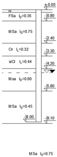
Figure 1.
Geotechnical profile at the location of an 8 m steel closed-end pipe-pile under testing.

Table 1.
Basic geotechnical parameters.
The pile used in the displacement test was constructed as a closed-end steel pipe, embedded in the ground by means of vibratory driving. Its diameter was 40 cm, total length equalled 8 m, and pipe wall thickness was 10 mm. It may be observed that pile toe is embedded in medium sand. Its capacity derived from the static calculation and considering the SLT exceeds 1500 kN. Test range was set to 1250 kN due to the limited capacity of anchoring piles and connections in the testing appliance.
The testing procedure was defined by the Polish Code of Practice [7] as a maintained load test with a constant rate of loading and maintained time (until settlement stabilization) at every loading step. Two load cycles were performed. The average time between consecutive load steps was 8 min in the first cycle and 11 min in the second cycle (Table 2).
Table 2.
Schedule of the conducted SLT.
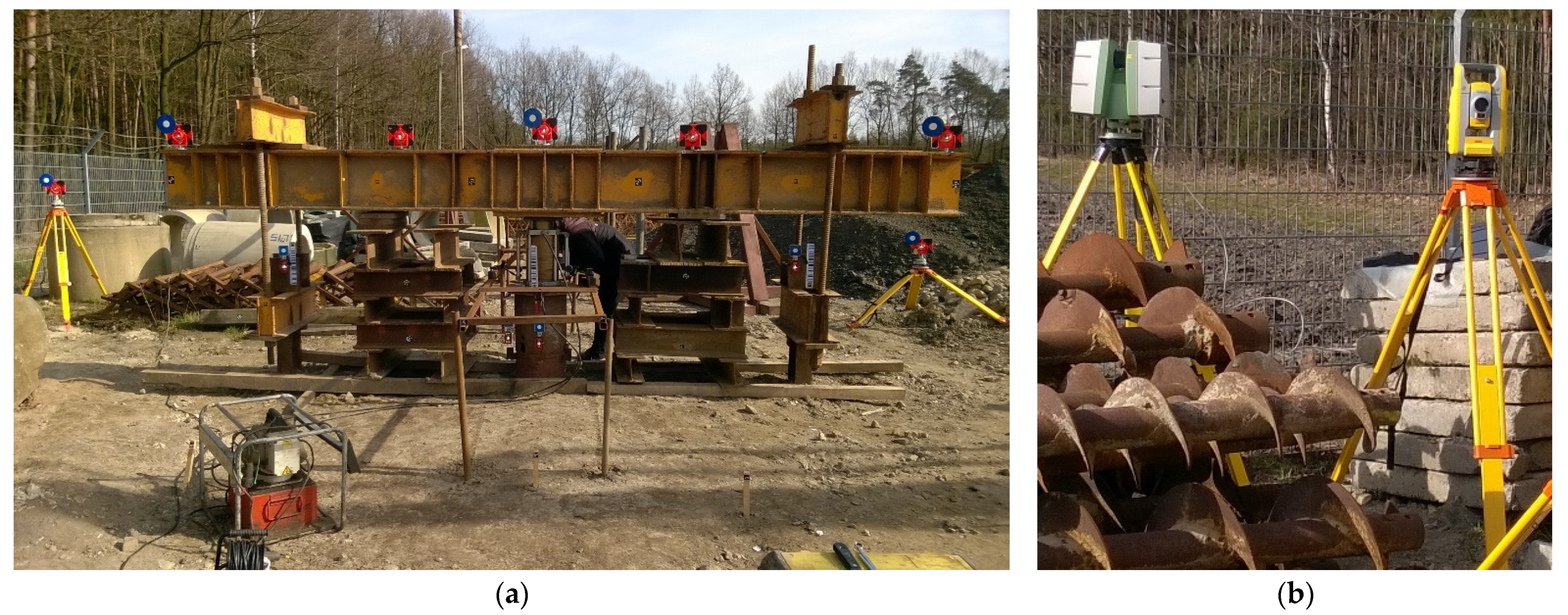
It must be emphasized here that other procedures of SLT, such as constant rate of penetration or constant time of loading at every step, do not change the applicability of the proposed procedure of inverse analysis. The loading scheme, with the reaction beam enabling the transfer of the loads to the anchoring piles (Figure 2a), predesignates the possibility of applying remote measurement methods (Figure 2b). If the load had to be transferred to a kentledge system, all measurements would be much more complicated due to the limited visibility and access to controlled points.
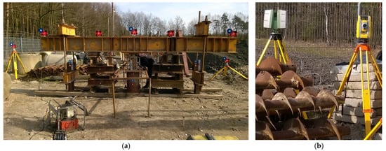
Figure 2.
View of the test stand and instrumentation: (a) the SLT appliance with attached dial gauges, prisms for total station, and planar targets for scanner; and (b) the position of the laser scanner and total station right in front of the loading structures.
The basic characteristics of the reaction beam are: 2 × HEB450, Jx = 2 × 79,890 [cm4], l = 4.166 [m], and E = 205 [GPa]. The beam was strengthened with 2 additional steel plates in its central part. Increased stiffness was considered in numerical studies of beam deflection.
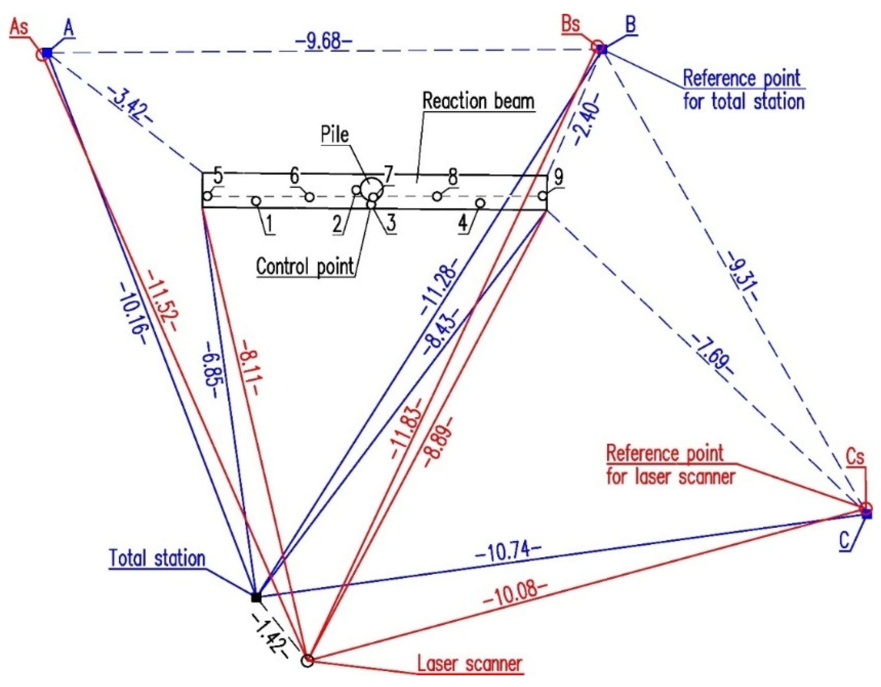
During the SLT, two geodetic methods were used. The first was precise tacheometry (trigonometrical heighting), the purpose of which was to determine the vertical displacements of key elements of the test stand (reaction beam, loaded pile, and anchor piles). Measurements were performed with a Trimble S3 robotic total station (Figure 2b) with an angle accuracy of 0.6 mgon and a distance measurement accuracy of ±2 mm + 2 ppm in the prism mode. The total station was situated at a distance of 6.85 m and 8.43 m from the ends of the reaction beam. The local reference system was established by three reference points (A, B, and C) located in the range of 10.16 ÷ 11.28 m from the instrument. The arrangement of the total station position and reference points ensured a favourable geometry of the referencing directions (Figure 3). The reference points were materialized by means of surveying prisms with a diameter of 62.5 mm and prism constant of −30 mm, mounted in tripods throughout the duration of the measurements (Figure 2a). The set of check points consisted of (Figure 2a):
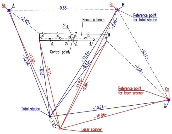
Figure 3.
Arrangement of measuring instruments and reference points.
- five points (numbers 5–9) located on the reaction beam and materialized by geodetic prisms with a diameter of 62.5 mm and prism constant of −30 mm;
- two points (numbers 2 and 3) attached to the side surface of the loaded pile and materialized by geodetic prisms with a diameter of 25.4 mm and prism constant of −16.9 mm; and
- two points (numbers 1 and 4) attached to the left and right anchor piles, respectively, and materialized by geodetic prisms with a diameter of 25.4 mm and prism constant of −16.9 mm.
The total station was remotely controlled by a TSC3 controller, in which the automatic series of measurements were defined. In each series, all prisms (A, B, C, and 1–9) were measured in two positions of the telescope (face left and face right) using the automatic target recognition system. The first series of measurements was made before starting the pile loading. Successive series were performed synchronously to the individual stages of pile loading during two loading cycles.
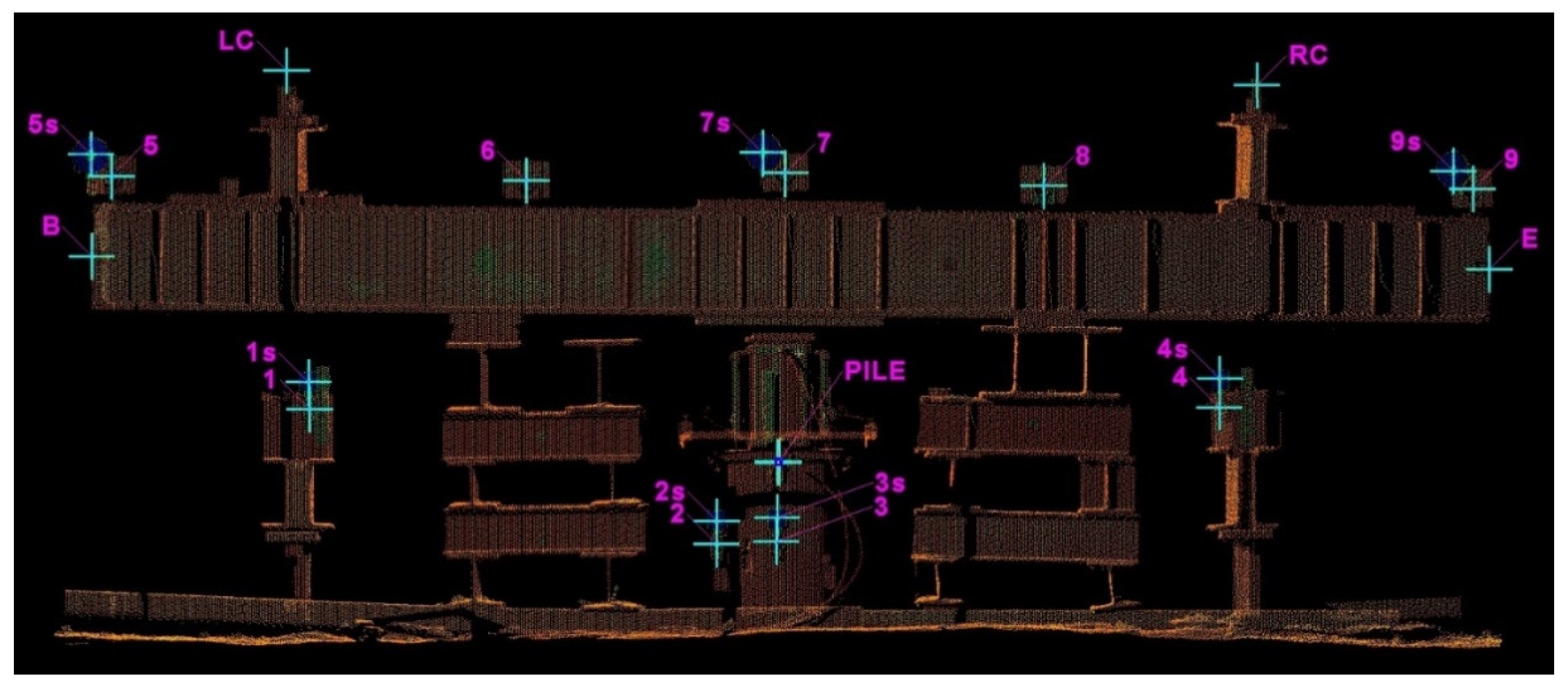
The second measurement method was terrestrial laser scanning (TLS), the purpose of which was to obtain precise data on the geometric shape of the reaction beam before loading. A Leica ScanStation C10 pulse laser scanner was used to carry out the measurements (Figure 2b). In the range of 50 m, the accuracy of a single angle, distance, and position measurement were 3.8 mgon, 4 mm, and 6 mm, respectively. According to the manufacturer, the precision of the modeled surface was 2 mm and the standard deviation of the target acquisition was 2 mm. The scanner position was located opposite to the reaction beam and tied-in to three reference points (As, Bs, and Cs), located in the vicinity of the test stand in the range of 10.08 ÷ 11.83 m (Figure 3). The reference points were materialized by circular planar targets in blue and white colours with a diameter of 6 inches. The set of check points consisted of (Figure 2a and Figure 4):
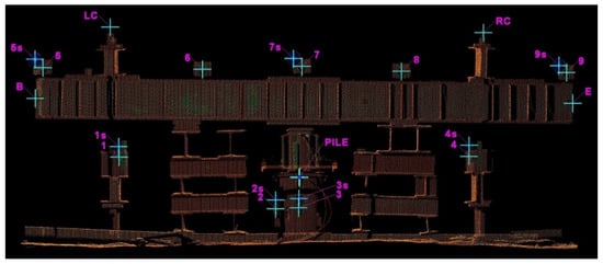
Figure 4.
Scanned test stand: schematic layout and numbering of check points.
- three points (number 5 s, 7 s, and 9 s) located on the reaction beam and materialized by circular planar targets in blue and white colours with a diameter of 6 inches;
- two points (number 2 s and 3 s) attached to the side surface of the loaded pile and materialized by square planar targets in blue and white colours with a dimension of 3 × 3 inches; and
- two points (number 1 s and 4 s) attached to the left and right anchor piles, respectively, and materialized by square planar targets in blue and white colours with a dimension of 3 × 3 inches.
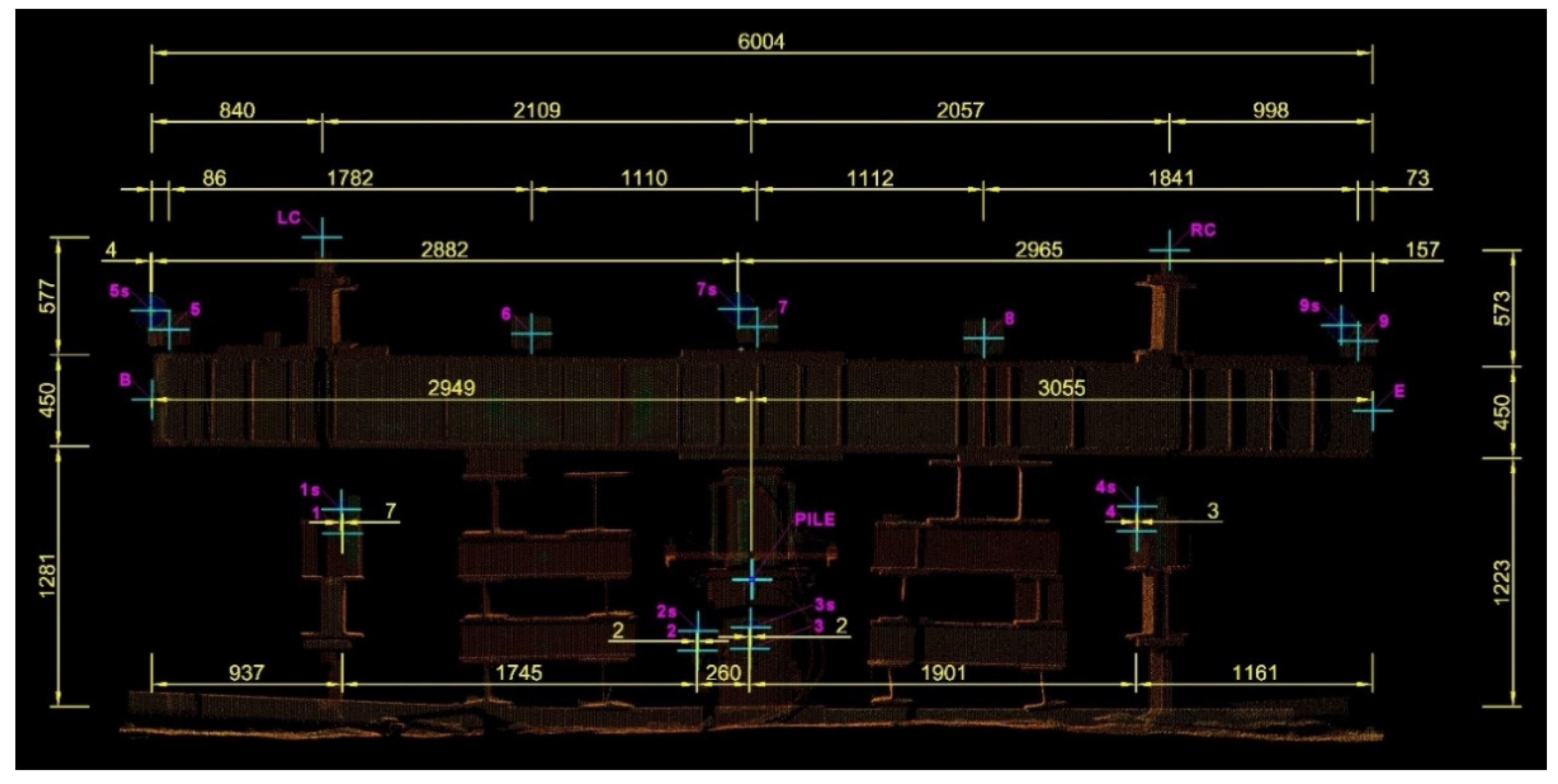
The laser scanner was controlled by laptop with Leica Cyclone software [8]. Before the pile loading started, a detailed scan of the whole test stand was performed. Additionally, all planar targets dedicated for the scanner were measured once with the total station. That made it possible to assign a common coordinate system to the measurement data from both instruments at a later stage. During the subsequent loading steps, only the planar targets were scanned in detail due to the limited scan speed (maximum instantaneous scan rate is 50,000 points per second) and short time per load step (few minutes). The dimensions describing the distribution of the controlled points on the test stand are shown in Figure 5.
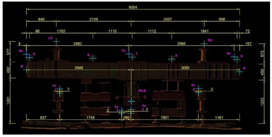
Figure 5.
Scanned test stand: distances between structure elements and measurement points.
2.2. Geodetic Techniques for Displacement Control
The determination of the displacement of natural objects and anthropogenic structure is the main task of engineering geodesy. Depending on the character of the object under scrutiny, there are different requirements in relation to: the dimension of displacement (1D, 2D, and 3D); the coordinate system (absolute or relative); the range of the expected displacement and requested accuracy; the availability of object (direct or remote measurements); and the dynamics of displacement changes and duration of the geodetic measurement. All these factors must be considered when selecting measurement methods and techniques. Geodetic methods are primarily aimed at providing an external coordinate system which is independent of the object under survey. This is an undoubted advantage but simultaneously is associated with limited accuracy. For comparison, physical methods have the accuracy of even a few orders of magnitude higher but they allow the registering of only relative displacements.
The most common applications of geodetic measurements in geotechnics include:
- measurements of vertical displacements (1D) of buildings in the vicinity of deep excavations and vertical displacements of the pile and anchor piles under testing during the SLT;
- measurements of horizontal displacements (2D) of the deep excavation wall and the piles during lateral test loads;
- measurements of spatial displacements (3D) of the retaining structures and landslides; and
- measurements of deformation of engineering structures (tailing ponds, tunnels, and bridges) and the surrounding area.
From the surveyor’s perspective, a displacement is a change in the position (coordinates) of selected check points representing the object in the assumed time interval in an external reference system, wherein the reference system is independent of the monitored object (“absolute” displacements). We can detect deformations when the mutual position of check points within the object under testing changes additionally. Then, the shape changes and the object does not move like a rigid body.
The classic method of determining vertical displacements is precision leveling, which allows for obtaining accuracy in tenths of a millimeter. An example of the application of this method in geotechnical monitoring can be found in [5,9,10,11,12].
Nowadays, horizontal displacement measurements are carried out using robotic total stations, sometimes combined with GNSS static measurements on reference points in extensive measurement networks. The common application of total station measurements described in the literature are landslide monitoring [13,14] and monitoring of a deep excavation in the urban space [15], as well as horizontal displacement control during the test of the pile lateral loading [16]. Total stations equipped with high-resolution cameras, called image assisted total stations (IATS), are increasingly used for vibration measurements [17,18]. The total station and GNSS receiver can also measure spatial displacements, although the spatial resolution of this measurement is very limited. Additionally, in the case of the GNSS technique, the measurement time is quite long and the accuracy is not very high. Conversely, the advantage is the ability to repeatedly measure the same well-defined points.
Nowadays, close-range photogrammetry is a very popular method to obtain 3D models describing the geometry of civil-engineering structures. In recent decades, photogrammetry has significantly evolved from the use of analog metric cameras (equipped with professional lenses with low image distortion) to digital cameras (even low-cost, non-metric) that try to compensate the imperfection of lenses with advanced calibration models. The algorithms for digital image processing and the automatic recognition of characteristic points in photos significantly increased the area of application, shortened the development time, and increased the accuracy of the results. The development of the technical capabilities of unmanned aerial vehicles (UAV) extends the field of photogrammetry applications to larger engineering facilities. An example of using UAV to acquire photos and then automatic detection of rail surface defects is presented in [19]. Photogrammetry and digital image correlation are widely used for 3D deformation measurements. Using the structure from the motion technique, we can generate point clouds comparable to those obtained from laser scanners. On the basis of the optimized displacement surfaces, it is possible to evaluate stress distributions using the boundary element method [20]. An example of using a digital image-based method for the deformation-monitoring of a steel truss–concrete composite beam during a static load test is described in [21]. The application of photogrammetry to assess the deformations of rod and plate elements of the steel constructions of hoisting machines is proposed in [22].
For at least a decade, terrestrial laser scanning has been widely used in the measurement of displacement and deformation. The continuous development of this technology allows for the increase in the accuracy, range, and speed of measurement. Depending on the type of laser scanner (continuous wave or pulsed) and specific model, the range varies from several dozen to several hundred meters, the accuracy ranges from a few to several millimeters, and the measurement speed can reach a million points per second. Due to the quasi-continuous mapping of the measured surfaces in the form of point clouds, TLS provides much more information about the shape of the object under scrutiny than the point measurement with a total station. The accuracy of the laser scanning in relation to the total station measurements was analyzed among others in [10,23,24,25]. In the matters related to monitoring, various measurement techniques are often combined, which allows for the collecting of a wider range of data and the building of multi-sensor-systems [26,27]. TLS is often used in the monitoring of displacements of landslides [28], in the retaining of structures [29,30,31,32], in mechanically stabilized earth walls [33], or in various types of hydrotechnical facilities [10,25,34,35]. Reliable stability analysis of the granite boulder on the basis of TLS data was described in [36]. The study of the deformation of tunnels, as well as of creating deformation models using data obtained from laser scanning, are very popular [37,38,39,40,41,42,43,44]. A slightly different issue that has been recently gaining popularity is the use of TLS to assess the roughness parameters of concrete surfaces interacting with the ground in geotechnical structures. Such analyses are performed with optical scanners on small samples in laboratory conditions [45,46,47] or with laser scanners on the construction site on a natural scale [29,31,48,49].
2.3. Geotechnical Testing Procedure
The constant rate of the load procedure was applied in accordance with the Polish Code of Practice [50]. After the assembling of the testing appliance (pile head, hydraulic jack, reference system for pile head displacement control, reaction beam, steel anchors, and reaction piles) and its instrumentation (dial gauges and controlled points with geodetic prisms and targets), the load was applied in stages to achieve the primarily assumed range. After unloading, the second round of loading was applied to check the pile’s behaviour under a cyclic loading. The main goal of the test according to [50] is to determine the load step, when pile settlements tend to arise and permanent settlements appear (and increase). The second goal of the test is to determine the so-called ultimate capacity, meaning the load that causes unstoppable and infinite settlement. This last value allows for the analysis of pile capacity according to [1]. If ultimate capacity is not used in the course of pile loading, various methods of test extrapolation can be applied; however, it always leads to some risk of inaccuracies. The authors’ previous studies proved that the reliability of extrapolation methods is highly dependent on the accuracy of displacement control at the last steps (stages of loading). The same doubts may arise concerning the accuracy of the force control and for that reason, the applied force range should be somehow controlled using an independent external system.
It is worth mentioning that piles used as anchors stabilizing the reaction beam are subject to large pulling forces. Their uplift may significantly change their behaviour (due to residual forces) in the course of standard loading under the building structure. That is why, at least in the Polish Code of Practice [50], the uplift of anchoring piles is limited to 5 mm. If that value is exceeded during the test, the anchoring pile is assumed to have only 80% of this designed load in compression. To avoid such a problem, current control of the anchoring pile uplift must be achieved and relevant modifications of the testing program may be applied.
Last but not least, one has to understand the difference between pile behaviour in compression (pushing towards the ground body) and its pulling resistance. In the case of typical axial loading by gravity forces, both pile shaft and base resistances are mobilized at various stages of the pile displacement. First, shaft resistance based on static frictional resistance and adhesion appear between the pile shaft and ground body. The range of pile displacement needed to mobilize this part of its capacity is close to 0.15% of its diameter. Mobilization of bottom resistance is based on a mechanism similar to shallow foundations with an appearance of plastic zones around the pile base. This part of the pile capacity is developed slowly and the full value of the base capacity is assumed to occur when its displacement ranges around 10% of the pile diameter.
The pile that is working in tension does not have any reserve of capacity resulting of base resistance. The capacity is achieved relatively suddenly (without warning) and it happens quite frequently that the anchoring pile jumps out of the ground in the course of the test. Such a situation is not acceptable because: (1) it violently stops the testing procedure before the designed range of load is achieved and (2) the anchoring pile that was “withdrawn” from the ground cannot be (in most cases, except precast driven piles) used in further construction.
That is why in both cases for the pile under testing and for the anchoring piles, excessive and even redundant measuring (controlling) techniques and systems are necessary and should be widely applied.
2.4. Inverse Analysis
Inverse analysis (or in other words, back-analysis) is a widely known procedure that enables the proper evaluation of stresses or forces acting on a structure on the basis of its deformation. In geotechnical engineering, inverse analysis is commonly used for the purpose of the so-called “observational method”, which consists of updating the computational model on the basis of the information achieved at earlier stages of loading. This method, devised by Terzaghi and Peck [51], was introduced mainly in the designing of deep excavations [52] in which problems of the proper evaluation of earth pressures create the need for partial validation and calibration of the computational model at subsequent stages of excavations. Earth pressures acting on soil-shell objects made of corrugated sheets may also be derived on the basis of back-analysis based on corrugated sheets’ deflection [53]. A similar procedure may be applied in tunneling works in which rock pressure on the tunnel lining may also be estimated based on internal shape deformation control.
This study advocates the inverse analysis for the evaluation of loading force during the SLT procedure. Here, both geometric characteristics of the element under load (e.g., constant moment of inertia J) as well as the elastic modulus of material E are known. Consider a well-known static equation for bend arrow f (1):
where F = applied force; f = bend arrow; a, b = distances to supports; and l = total length of the beam, wherein l = a + b (Figure 6).
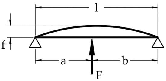
Figure 6.
Static scheme of the beam loaded non-centrically.
A proper approximation of both the geometry of the beam and its deflection at every stage of loading make it possible to derive the value of the loading force according to Equation (2):
3. Results
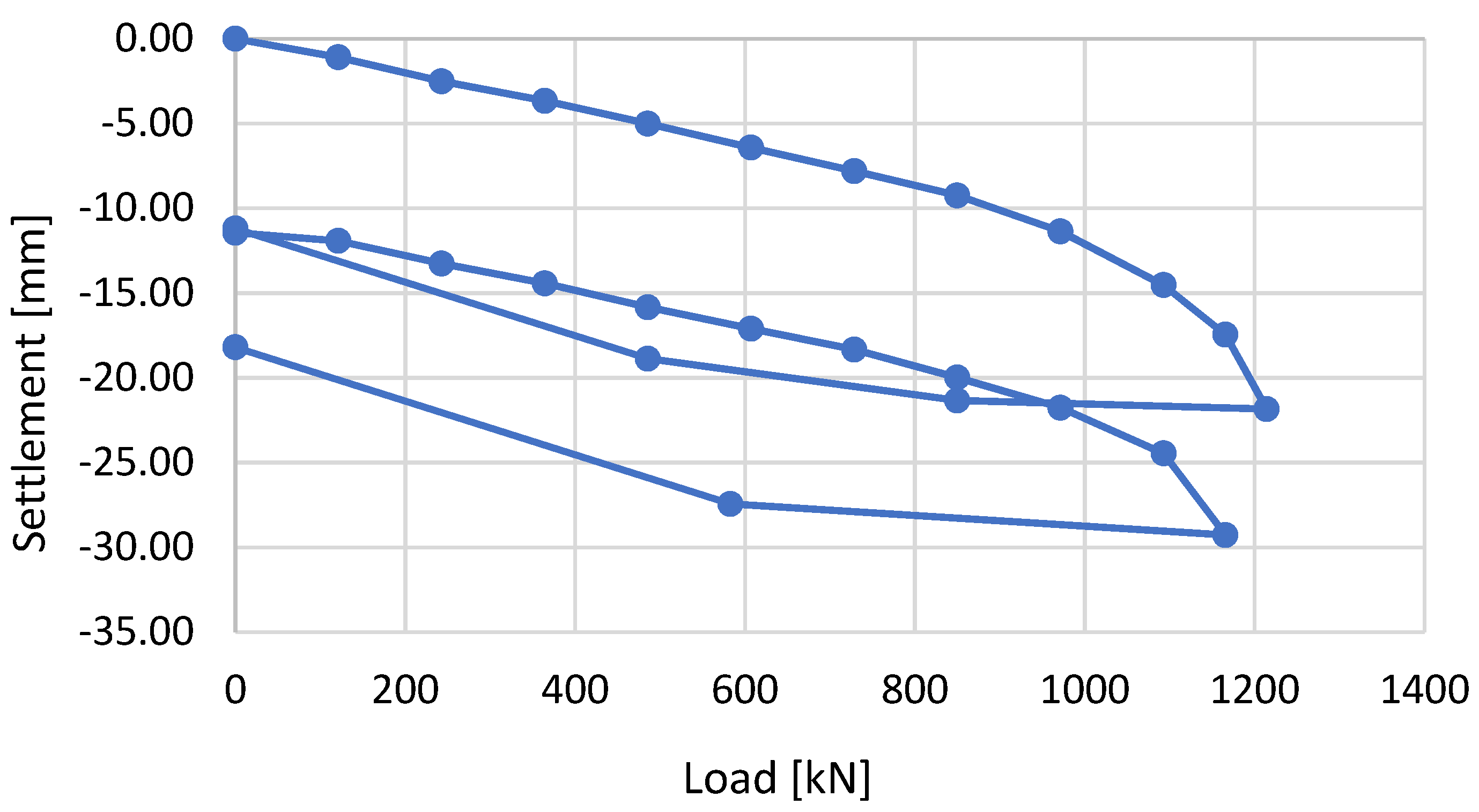
The entire test was performed in two cycles and many stages. The pile was loaded and unloaded in constant steps. Two independent issues were controlled simultaneously by means of dial gauges and remote geodetic methods in the course of the test. Pile settlements from dial gauges are presented in Figure 7. It may be observed that the pile settlement range is within 30 mm (in 2 cycles). The expected beam deflection was also within the same range of 30 mm (both values had to be pre-assessed for proper selection of the hydraulic jack, considering its piston length, which was equal to 150 mm).

Figure 7.
Load versus settlement curve from the SLT in two cycles of loading on the basis of dial gauges measurement.
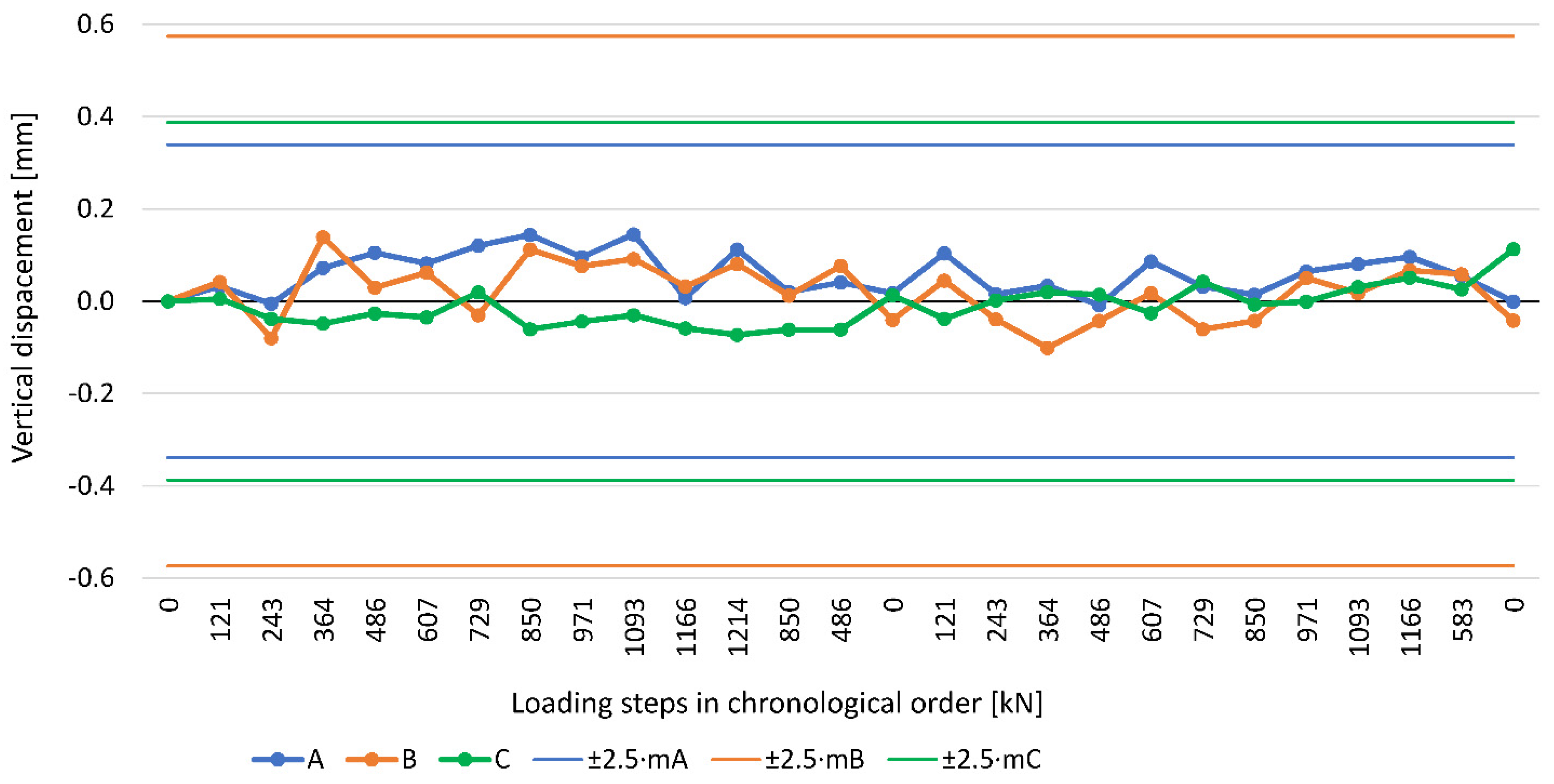
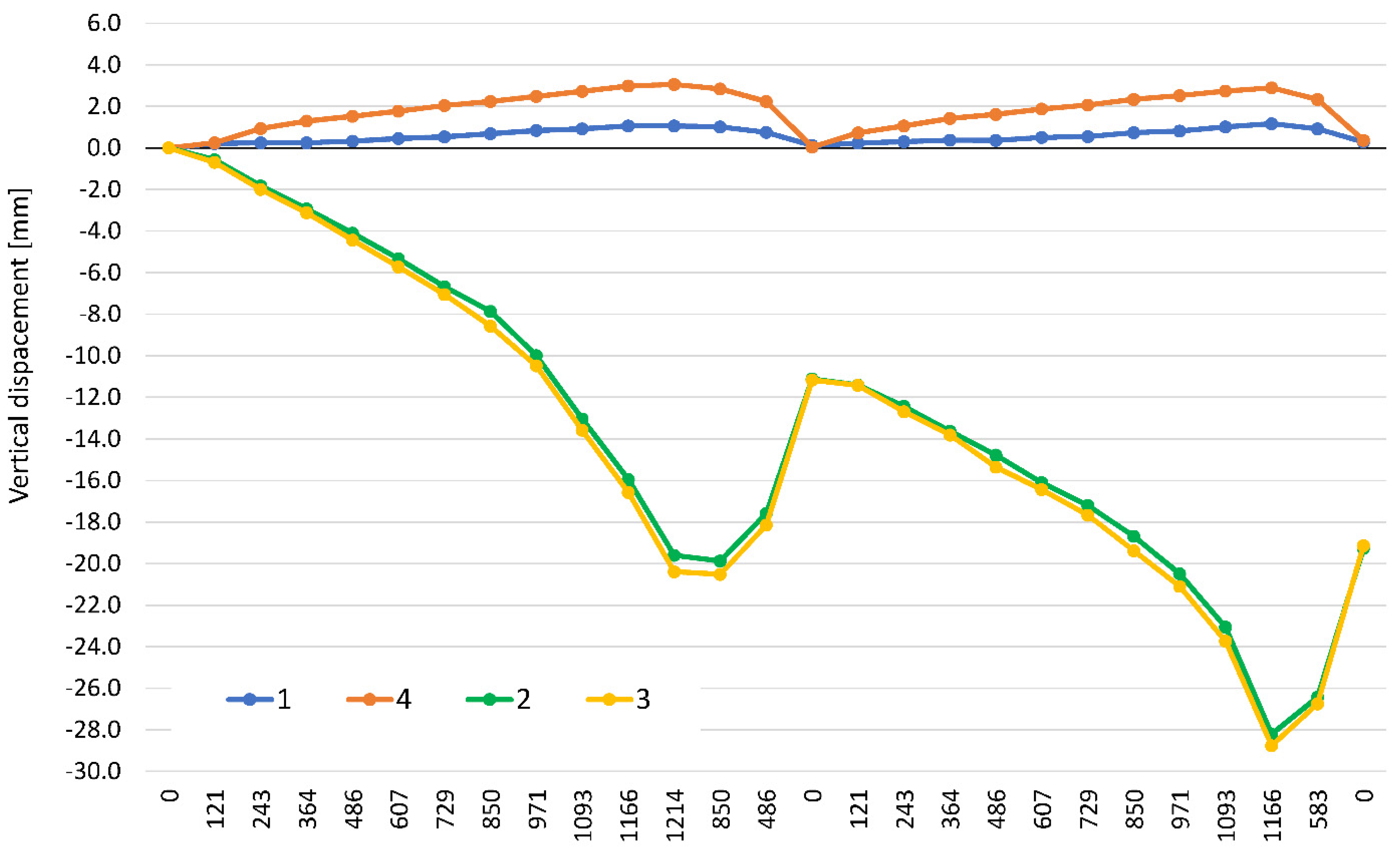
The elaboration of the results of geodetic measurements began with the control of the stability of reference points. The “apparent” displacements of the points A, B, and C do not exceed the interval of 2.5 times in mean errors in their determination; therefore, they fall within the measurement noise and the reference points can be treated as a constant in time (Figure 8). On the basis of the data from total station measurements, the heights of the controlled points for individual epochs were calculated using the trigonometric leveling method. Treating the first epoch as an initial measurement, the vertical displacements of all control points were calculated. Figure 9 shows the lifting of anchor piles and the settlement of the tested pile during the SLT. The beam deflection observed in cycle 1 and cycle 2 is shown in Figure 10a,b, respectively.
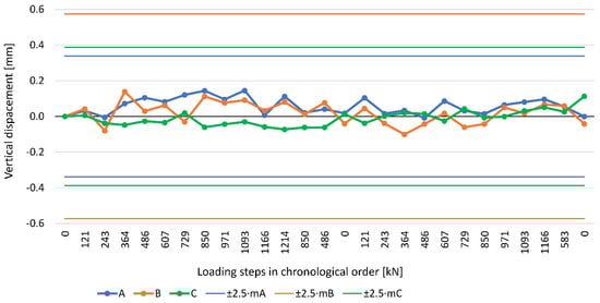
Figure 8.
“Apparent” vertical displacement (measurement noise) of reference points: A, B, and C during first and second loading cycles with an acceptable range of ±2.5·mA, ±2.5·mB, and ±2.5·mC (two and a half times the mean error of vertical displacement determination for each reference point).

Figure 9.
Vertical displacement of check points: 1 = left anchor pile, 2 and 3 = loaded pile, and 4= right anchor pile.
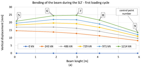
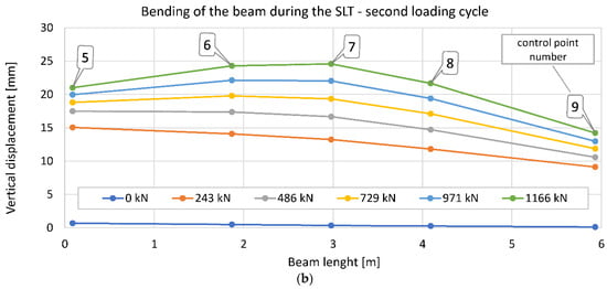
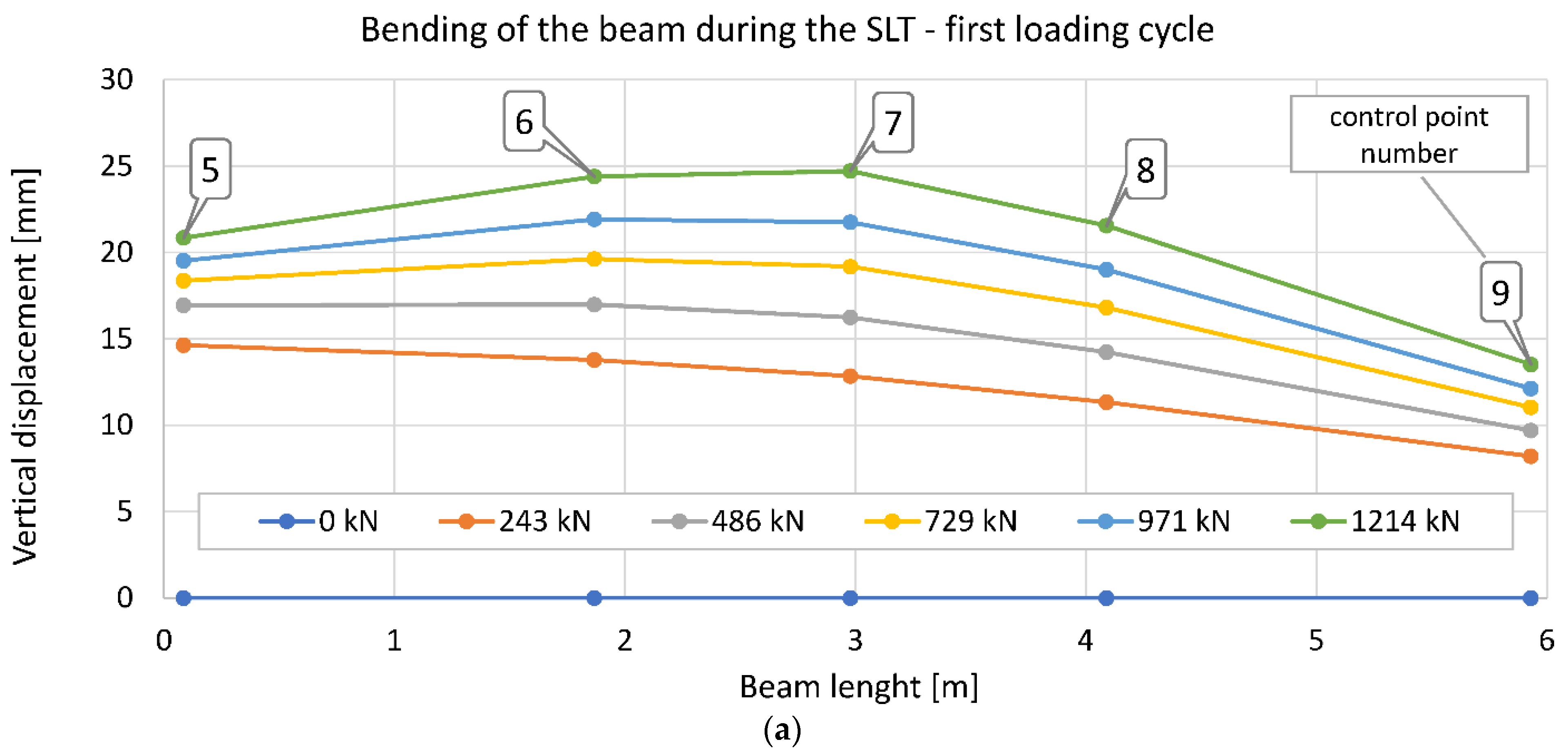
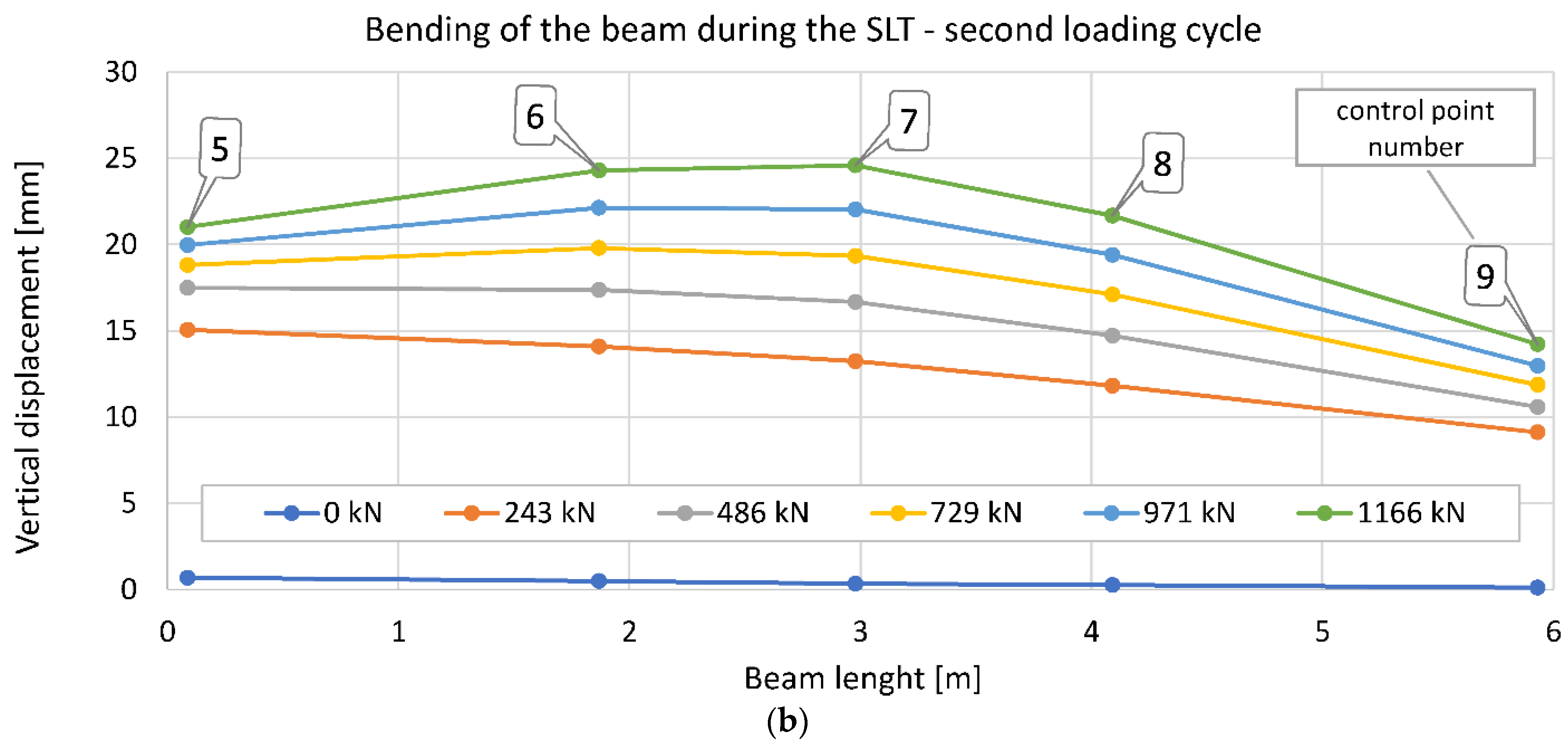
Figure 10.
Bending of the beam during the SLT on the basis of vertical displacement in control points numbers 5–9 from Trimble S3: (a) first loading cycle and (b) second loading cycle.
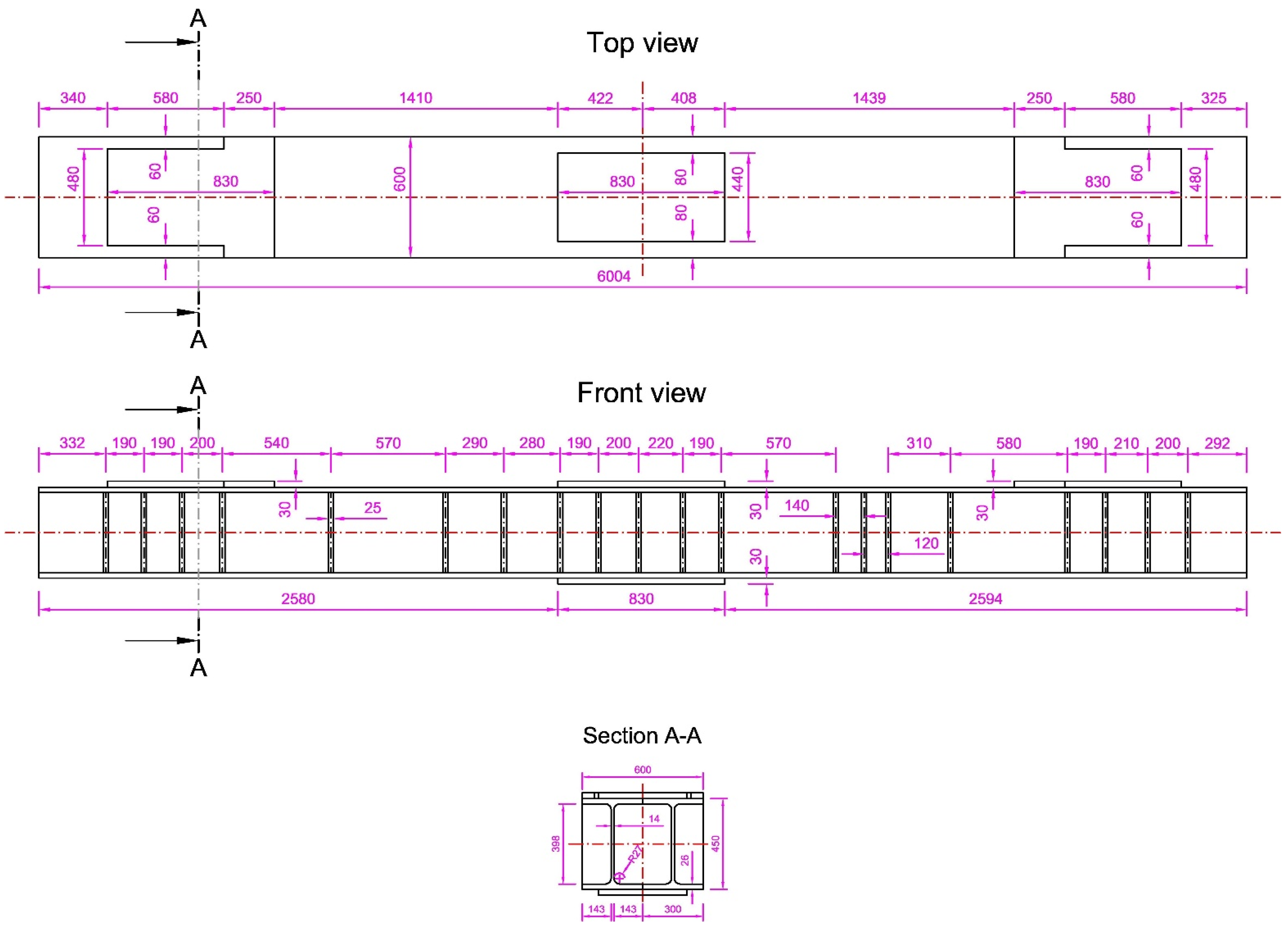
On the basis of the point cloud from laser scanning, the detailed beam geometry data was obtained, which are shown in Figure 11.
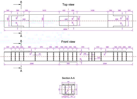
Figure 11.
The dimensions of the reaction beam (top view, front view, and section A-A).
The pile settlement is not the main subject of current study as the problem of its credibility was discussed in former sources (including authors’ contributions [4,5,10,16]). Only the relevance of the load measured indirectly by the control of oil pressure in the hydraulic system is being checked by back-analysis of the steel beam deflection.
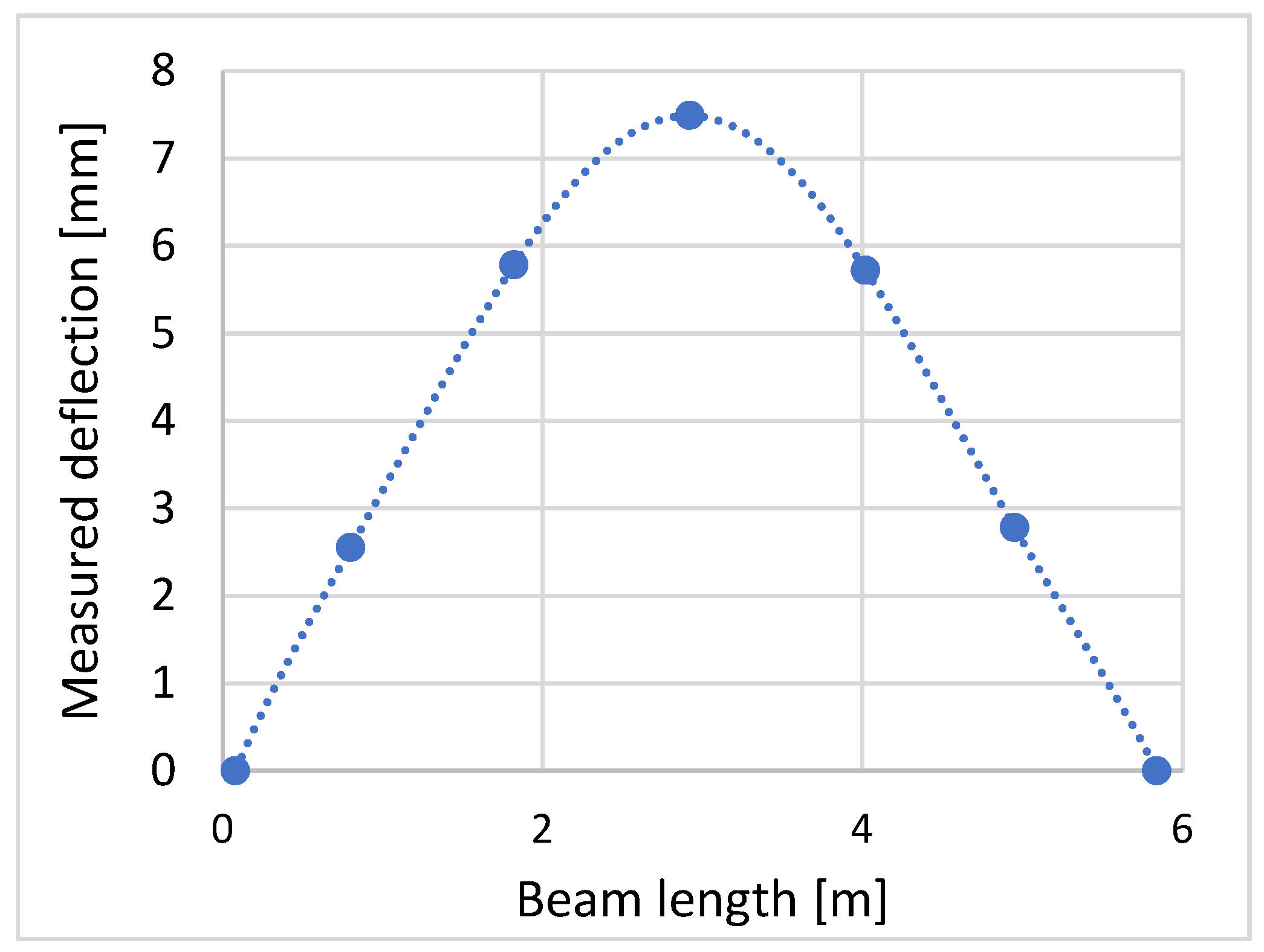
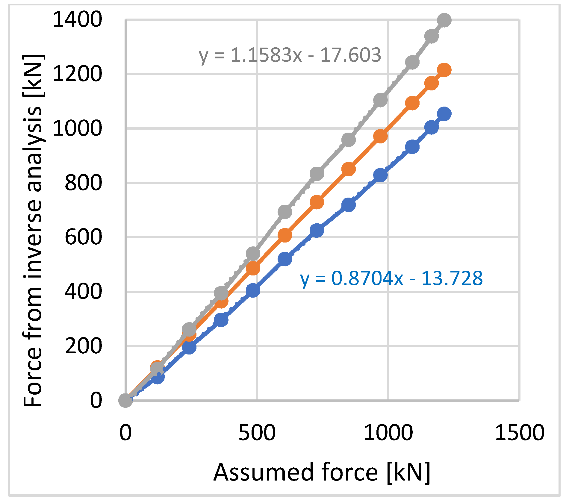
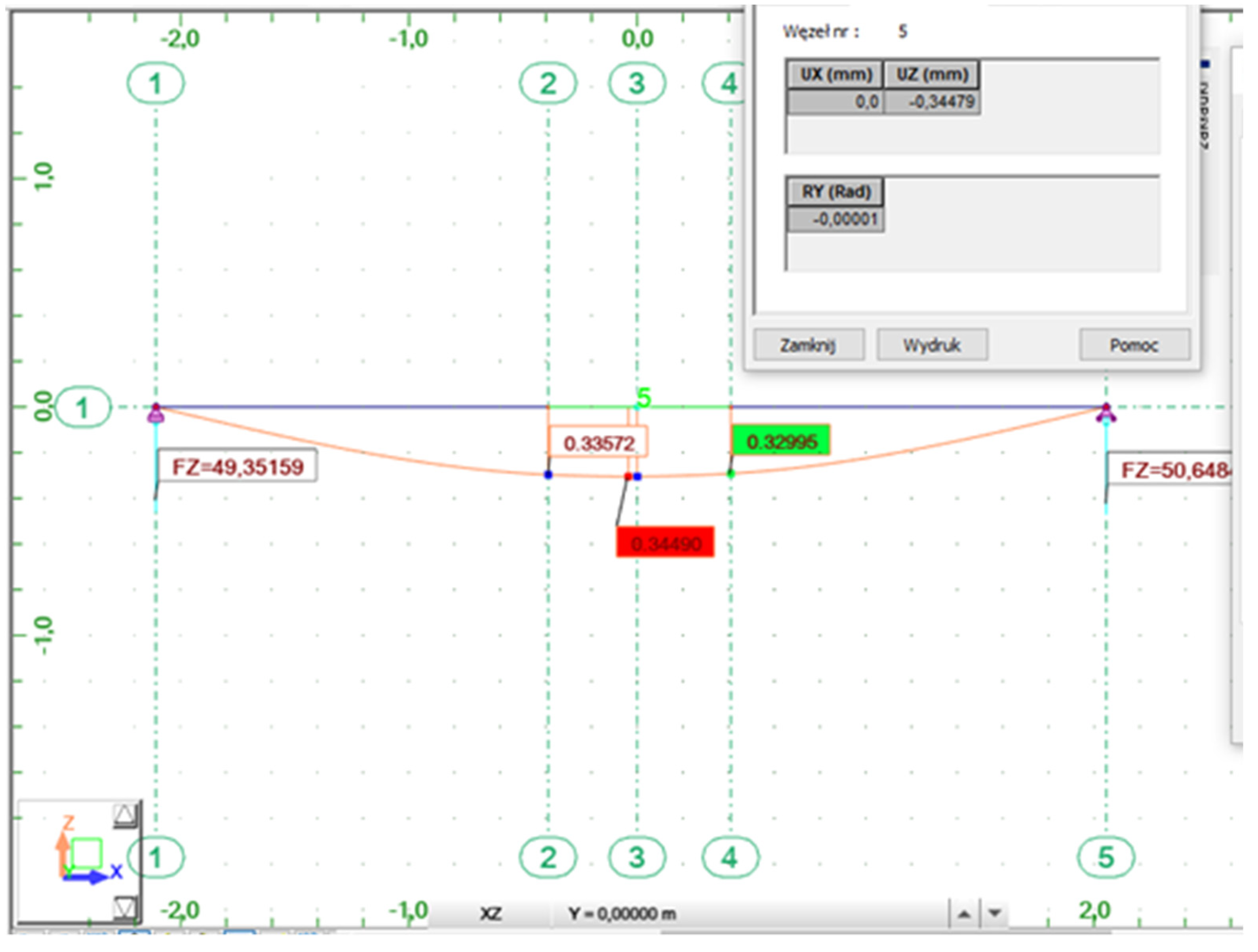
Looking at Figure 10, we may observe that the deflection raises at every load step and reaches its magnitude in point 7, directly over the piston. As the elastic modulus of the construction steel is rather a constant value, it must be the geometry that is potentially responsible for the lower displacements (deflections); see Figure 11. Let us consider now the shape of the deflected beam at every stage of two cycles of pile loading. Figure 12 represents the shape of the deflected beam at the last step (i.e., the highest load value) of the first load cycle. If we measure the bend arrow by means of geodetic methods, the loading force can be easily back-calculated and compared to the force derived from the hydraulic jack characteristics on the basis of the oil pressure control. We can just compare the bend arrow in point 7, measured on the basis of remote geodetic measurements, with the results of theoretical equations and numerical studies concerning the precise geometry and stiffness of bended elements. In this way, we may notice that the force causing deflection must have been smaller than the one derived from the hydraulic actuator characteristics or that the beam must have been stiffer than assumed for the computation. Figure 13 shows the relationship between the forces: the assumed value (from pressure) versus the force obtained from the inverse analysis. The result (blue line) seems to be alarming but it must be considered that the simplified Equation (1) assumes constant stiffness along the beam. In reality, the beam was reinforced in its central part with an upper and lower steel plate. The increased stiffness in the central part diminished the deflection. New computation using the dedicated software Robot Structural Analysis [54] for static analysis (Figure 14, Figure 15 and Figure 16) showed that the magnitude of deflection (bend arrow) may be computed from the following equation, Equation (3) (see: Figure 16). For the measured value of displacement equal to f = 4.82 mm, using the transformed Equation (4), we achieve a value of F = 1397.51 kN.
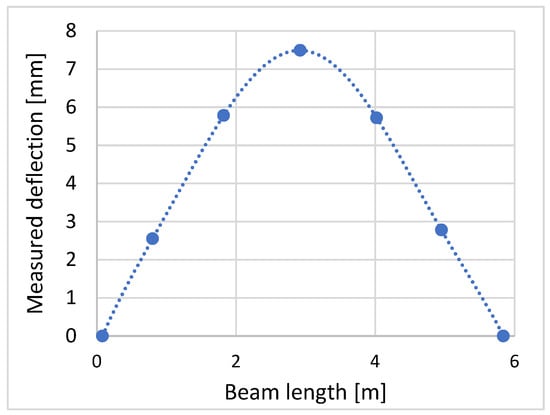
Figure 12.
Simplified shape of the deflected beam between supports.
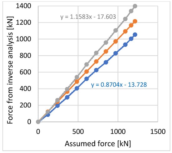
Figure 13.
Comparison of forces: assumed value (orange line) versus the force from inverse analysis in a simplified model (blue line) and in numerical studies with appropriate beam stiffness (grey line).
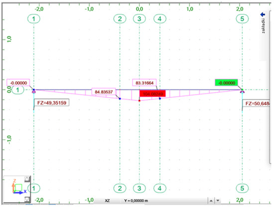
Figure 14.
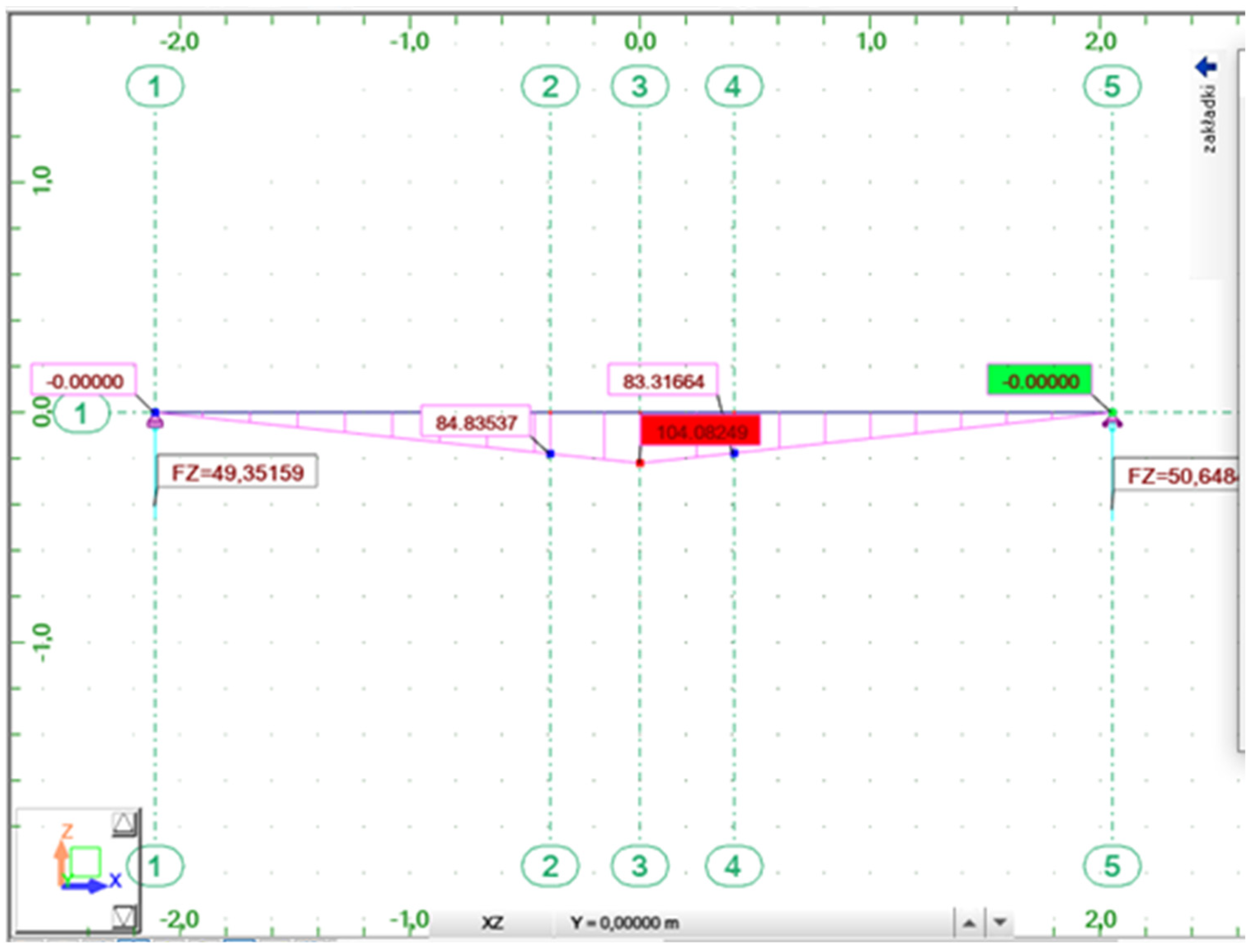
Bending moment of the main beam with an increased stiffness in the central part.
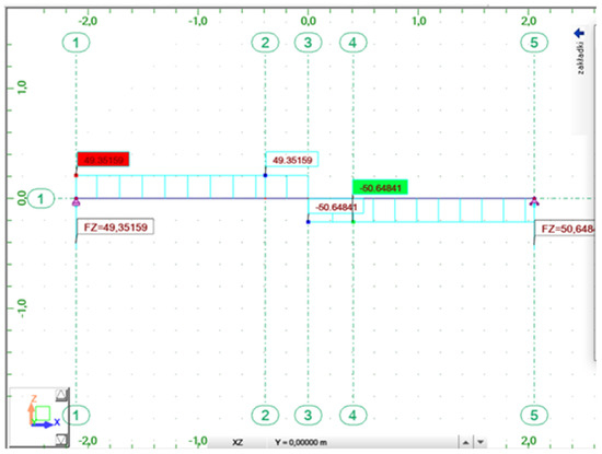
Figure 15.
Shear forces of the beam with an increased stiffness in the central part. Point load equal to 100 kN.
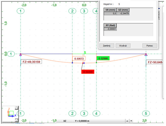
Figure 16.
Shape of the deflected beam with an increased stiffness in the central part. Point load equal to 100 kN.
4. Discussion
The measured deflections of the steel beam in the first and second loading cycles are presented in Figure 10. The values of the force that impose such a deflection shape at the subsequent steps of the first cycle are given in Figure 13, versus the load derived from the pressure in the hydraulic system.
The apparent load seems to be overestimated within the range of 13% (if we apply the simplified model of the beam, neglecting additional steel plates). The results of calculations considering the increased stiffness in the central part of the beam give surprising results, meaning that the force causing the observed range of deflection must have been higher (within a range of 15%) than the value derived from the oil pressure in the hydraulic system (see Figure 14, Figure 15 and Figure 16 in which bending moments, shear forces, and finally beam deflections are given for a value of loading force equal to F = 100 kN). Due to the linear dependence between force and bend arrow, similar values may be achieved for other load cycles. However, a more sophisticated analysis based on numerical calculations of deflections shows that the increased stiffness in the central part of the beam (due to the additional steel plates welded-in) may practically have a smaller effect because welding at plate edges does not provide full assembling and its effect may be smaller than it was assumed. If we assume that plates are not fully welded, we receive from numerical calculations that f = 0.0044787·F and consequently F = 224.28·f, which seems to underestimate the value of the force applied.
Stress control could be an alternative way to validate the applied force. Both methods (based on stress control and geodetic measurements of shape deflection) can be used simultaneously to provide a higher reliability of results. It is important to realize that the accuracy of both methods depends on proper evaluation of beam stiffness. This study shows just one of the possibilities, namely, the one that allows for providing force control from a certain distance. Through this way or another, numerical analysis proceeded with proper instrumentation of the testing appliance and reliable remote geodetic techniques increased the creditability of results.
It is evident that the measured values of displacement and deflection of the reaction beam make it possible to “calculate backwards” the force applied at every load step. The equation given in Figure 13 proves that, in field conditions, the observed increase or decrease of the loading force in comparison to the value computed from the hydraulic jack characteristics on the basis of the measured pressure may reach over 15%. The constant value of approximately 14 kN may be also related to the unexpected shear applied to the piston or the pressure loss between the manometer and the piston. The measurement of force during the SLT of a foundation pile can be “to some extent validated” by the inverse analysis of the deformation of a steel structure intended to ensure the transfer of force to the anchor piles. The presented study shows, however, that a simplified model of the beam should not be used as the inverse analysis procedure results are very much dependent on the real beam stiffness. In the final stage of loading of the pile under testing, achieving the planned (in numerical computations) beam deflection guarantees that the test is carried out in the required load range. It must be emphasized that the underestimation or overestimation of loading force even within a range of 15% does not seriously affect the SLT result (as a quality control procedure of a single pile). However, the SLT can also be carried out just in the way of acquiring information about soil parameters for a further pile design. In that case, any overestimation of geotechnical parameters (soil capacity) may be directly transferred to the design project and badly affect the creditability of the static calculation and reliability of the design.
Last but not least, apart from controlling the shape of the deflected beam, a continuously controlled uplift of the anchoring piles (Figure 9) makes it possible to meet the conditions of the Code [50], concerning the allowable values of anchoring piles’ uplift in the course of the test. This underestimated issue has severe consequences if neither addressed nor dealt with, as the Code [50] admits only 80% of derived capacity for the anchoring pile working under the structure. In the conducted SLT, the lifting of the anchor piles was not uniform. The right anchor pile had lifted a maximum of 3.1 mm and therefore had not exceeded the 5 mm limit.
The bending of the load beam was analyzed on the basis of point (discontinuous) data, obtained from the tacheometer measurement. If a faster and more accurate laser scanner was used, it would be possible to obtain a point cloud describing the beam shape from individual loading steps. Such studies are planned for the future.
5. Conclusions
This study is a pioneering work concerning the application of remote geodetic techniques for loading force control in the course of the SLT of foundation piles, as only a few references could be found (mainly by private communication). The present case study just confirms the suitability of robotic tacheometry and TLS as an additional way of providing creditable information on both values controlled during an SLT: pile head displacement (that is evident as remote control provides higher reliability of measurements, despite slightly lower accuracy in comparison with dial gauges) and loading force (in the condition that proper evaluation of beam stiffness is carried out). The control of the anchoring piles’ uplift is just an added value. The authors understand the complexity of the transmission of geodetic monitoring results to the applied force range in the test. It is inevitable, however, that even if the alert (warning) is not provided in the course of field test, creditable data may help to properly compute pile capacity in further post-processing of field test results. The authors’ earlier studies (placed in the reference list) highlighted the importance of a proper evaluation of the SLT conduct at the last stages of loading that are decisive for proper capacity evaluation. It is a negative coincidence that the faults in the evaluation of settlement (due to the unstable reference system for dial gauges) and load (due to the underestimated or even neglected friction between the piston and actuator body) may appear on the most important final steps of the testing procedure.
It must be emphasized that the SLT itself is a very costly testing procedure. All phenomena related to loading and unloading within a range far exceeding the working load of the pile (occasionally reaching the pile’s capacity) make it impossible to repeat the procedure in a short time. A potential failure or damage of the manometer or any other problem in the hydraulic system (e.g., in hydraulic jack or connections of pressure hose) results in a long delay or in lower creditability of the repeated test. The application of geodetic remote measurement techniques helps to overcome this issue. In the same way, it helps to provide information about the pile head settlement in the event of failure of the reference system for measuring the displacement of the pile under testing or the uplift of anchor piles.
Prospects for new developments and the need for validation for a larger number of SLTs must be emphasized, and numerous further instrumented pile tests are planned in the near future.
Author Contributions
Conceptualization, Z.M. and J.R.; methodology, Z.M. and J.R.; software, Z.M. and J.R.; validation, Z.M. and J.R.; formal analysis, Z.M. and J.R.; investigation, Z.M.; resources, Z.M. and J.R.; data curation, Z.M.; writing—original draft preparation, Z.M. and J.R.; writing—review and editing, Z.M. and J.R.; visualization, Z.M.; supervision, Z.M. and J.R.; project administration, Z.M. and J.R.; funding acquisition, Z.M. and J.R. All authors have read and agreed to the published version of the manuscript.
Funding
This research received no external funding. 27% of article processing charge (APC) was paid from the budget of the Department of Geodesy and Geoinformatics at the Faculty of Geoengineering, Mining and Geology at Wrocław University of Science and Technology, Wrocław, Poland.
Acknowledgments
Authors would like to express their gratitude to PPI Chrobok S.A. for their kind assistance in assembling all testing appliances for field studies. Authors would also like to express their gratitude to Hubert Szabowicz and Jakub Rainer for their kind assistance in numerical modelling used for the current study.
Conflicts of Interest
The authors declare no conflict of interest.
References
- European Committee for Standardization. EN 1997-1 Eurocode 7: Geotechnical Design—Part 1: General Rules; European Committee for Standardization: Brusseles, Belgium, 2009. [Google Scholar]
- Fellenius, B.H. Basics of Foundation Design—A Textbook; Electronic. BiTech Publishers Ltd.: Richmond, BC, Canada, 2019. [Google Scholar]
- Matsumoto, T.; Matsuzawa, K.; Kitiyodom, P. A role of pile load test—Pile load test as element test for design of foundation system. In The Application of Stress-Wave Theory to Piles: Science, Technology and Practice, Proceedings of the 8th International Conference on the Application of Stress-Wave Theory to Piles, Lisbon, Portugal, 8–10 September 2008; ResearchGate: Berlin, Germany, 2008; pp. 8–10. [Google Scholar]
- Baca, M.; Muszyński, Z.; Rybak, J.; Żyrek, T. The application of geodetic methods for displacement control in the self-balanced pile capacity testing instrument. In Advances and Trends in Engineering Sciences and Technologies, Proceedings of the International Conference on Engineering Sciences and Technologies, Tatranská Štrba, Slovakia, 27–29 May 2015; Al Ali, M., Platko, P., Eds.; Leiden/CRC Press/Balkema: Tatranská Štrba, Slovakia, 2016; pp. 15–20. [Google Scholar] [CrossRef]
- Muszyński, Z.; Rybak, J. Some remarks on geodetic survey methods application in displacement measurements and capacity testing of injected and driven piles. In Proceedings of the 14th International Multidisciplinary Scientific Geo Conference (SGEM 2014), Surveying Geology and Mining Ecology Management, Albena, Bulgaria, 17–26 June 2014; Volume 2, pp. 451–458. [Google Scholar] [CrossRef]
- Tkaczyński, G. Personal communication. 2019. [Google Scholar]
- Polish Committee for Standardization (PKN). PN-B-02482:1955. Building Foundations—Load Bearing Capacity of Piles and Pile foundations—Guideline Determination; PKN: Warsaw, Poland, 1955. (In Polish) [Google Scholar]
- Cyclone, Version 9.3.1 64-bit; Leica Geosystems AG: Heerbrugg, Switzerland, 2018.
- Shults, R. Development and research of the methods for analysis of geodetic monitoring results for the subway tunnels. In Proceedings of the 4th Joint International Symposium on Deformation Monitoring (JISDM), Athens, Greece, 15–17 May 2019. [Google Scholar]
- Muszyński, Z.; Rybak, J. Evaluation of Terrestrial Laser Scanner Accuracy in the Control of Hydrotechnical Structures. Stud. Geotech. Mech. 2017, 39, 45–57. [Google Scholar] [CrossRef] [Green Version]
- Lõhmus, H.; Ellmann, A.; Märdla, S.; Idnurm, S. Terrestrial laser scanning for the monitoring of bridge load tests–two case studies. Surv. Rev. 2018, 50, 270–284. [Google Scholar] [CrossRef]
- Caroti, G.; Piemonte, A.; Squeglia, N.; Italia, L.P.; Italia, L.P. 100 Years of Geodetic Measurements in the Piazza del Duomo (Pisa, Italy): Reference Systems, Data Comparability and Geotechnical Monitoring. In Proceedings of the 4th Joint International Symposium on Deformation Monitoring (JISDM), Athens, Greece, 15–17 May 2019. [Google Scholar]
- Gumilar, I.; Fattah, A.; Abidin, H.Z.; Sadarviana, V.; Putri, N.S.E. Kristianto Landslide monitoring using terrestrial laser scanner and robotic total station in Rancabali, West Java (Indonesia). In AIP Conference Proceedings, Proceedings of the 6th International Symposium on Earth Hazard and Disaster Mitigation (ISEDM 2016), Bandung, Indonesia, 11–12 October, 2016; American Institute of Physics Inc.: Melville, NY, USA, 2017; Volume 1857. [Google Scholar]
- Artese, S.; Perrelli, M. Monitoring a landslide with high accuracy by total station: A DTM-based model to correct for the atmospheric effects. Geoscience 2018, 8, 46. [Google Scholar] [CrossRef] [Green Version]
- Ghorbani, E.; Khodaparast, M. Geodetic Accuracy in Observational Construction of an Excavation Stabilized by Top-Down Method: A Case Study. Geotech. Geol. Eng. 2019, 37, 4759–4775. [Google Scholar] [CrossRef]
- Muszyński, Z.; Rybak, J. Horizontal Displacement Control in Course of Lateral Loading of a Pile in a Slope. Proc. IOP Conf. Ser. Mater. Sci. Eng. 2017, 245, 032002. [Google Scholar] [CrossRef]
- Ehrhart, M.; Lienhart, W. Monitoring of Civil Engineering Structures using a State-of-the-art Image Assisted Total Station. J. Appl. Geod. 2015, 9, 174–182. [Google Scholar] [CrossRef]
- Lienhart, W.; Ehrhart, M.; Grick, M. High frequent total station measurements for the monitoring of bridge vibrations. J. Appl. Geod. 2017, 11, 1–8. [Google Scholar] [CrossRef]
- Wu, Y.; Qin, Y.; Wang, Z.; Jia, L. A UAV-based visual inspection method for rail surface defects. Appl. Sci. 2018, 8, 1028. [Google Scholar] [CrossRef] [Green Version]
- Honório, L.M.; Pinto, M.F.; Hillesheim, M.J.; De Araújo, F.C.; Santos, A.B.; Soares, D. Photogrammetric Process to Monitor Stress Fields Inside Structural Systems. Sensors 2021, 21, 4023. [Google Scholar] [CrossRef] [PubMed]
- Chu, X.; Zhou, Z.; Deng, G.; Duan, X.; Jiang, X. An Overall Deformation Monitoring Method of Structure Based on Tracking Deformation Contour. Appl. Sci. 2019, 9, 4532. [Google Scholar] [CrossRef] [Green Version]
- Yu Ganshkevich, A.; Shikhov, N.S.; Stoyantsov, N.M. Estimation of deformations of steel constructions of cranes based on photogrammetry. J. Phys. Conf. Ser. 2021, 1926, 012061. [Google Scholar] [CrossRef]
- Muszyński, Z.; Rybak, J.; Kaczor, P. Accuracy Assessment of Semi-Automatic Measuring Techniques Applied to Displacement Control in Self-Balanced Pile Capacity Testing Appliance. Sensors 2018, 18, 4067. [Google Scholar] [CrossRef] [Green Version]
- Xu, X.; Bureick, J.; Yang, H.; Neumann, I. TLS-based composite structure deformation analysis validated with laser tracker. Compos. Struct. 2018, 202, 60–65. [Google Scholar] [CrossRef]
- Muszyński, Z. Assessment of suitability of terrestrial laser scanning for determining displacements of cofferdam during modernization works on the Rędzin sluice. In Proceedings of the 14th International Multidisciplinary Scientific Geo Conference (SGEM 2014), Surveying Geology and Mining Ecology Management, Albena, Bulgaria, 14–22 August 2014; Volume 2, pp. 81–88. [Google Scholar] [CrossRef]
- Erol, B. Evaluation of high-precision sensors in structural monitoring. Sensors 2010, 10, 10803–10827. [Google Scholar] [CrossRef] [Green Version]
- Stenz, U.; Hartmann, J.; Paffenholz, J.A.; Neumann, I. High-precision 3D object capturing with static and kinematic terrestrial laser scanning in industrial applications-approaches of quality assessment. Remote Sens. 2020, 12, 290. [Google Scholar] [CrossRef] [Green Version]
- Barbarella, M.; Fiani, M.; Lugli, A. Landslide monitoring using multitemporal terrestrial laser scanning for ground displacement analysis. Geomat. Nat. Hazards Risk 2015, 6, 398–418. [Google Scholar] [CrossRef]
- Seo, H. Long-term Monitoring of zigzag-shaped concrete panel in retaining structure using laser scanning and analysis of influencing factors. Opt. Lasers Eng. 2021, 139, 106498. [Google Scholar] [CrossRef]
- Oskouie, P.; Becerik-Gerber, B.; Soibelman, L. Automated measurement of highway retaining wall displacements using terrestrial laser scanners. Autom. Constr. 2016, 65, 86–101. [Google Scholar] [CrossRef]
- Seo, H.J.; Zhao, Y.; Wang, J. Monitoring of Retaining Structures on an Open Excavation Site with 3D Laser Scanning. In Proceedings of the International Conference on Smart Infrastructure and Construction 2019 (ICSIC), Cambridge, UK, 8–10 July 2019; ICE Publishing: London, UK, 2019; pp. 665–672. [Google Scholar]
- Seo, H. Tilt mapping for zigzag-shaped concrete panel in retaining structure using terrestrial laser scanning. J. Civ. Struct. Heal. Monit. 2021, 11, 851–865. [Google Scholar] [CrossRef]
- Lin, Y.-J.; Habib, A.; Bullock, D.; Prezzi, M. Application of High-Resolution Terrestrial Laser Scanning to Monitor the Performance of Mechanically Stabilized Earth Walls with Precast Concrete Panels. J. Perform. Constr. Facil. 2019, 33, 04019054. [Google Scholar] [CrossRef]
- Alba, M.; Fregonese, L.; Prandi, F.; Scaioni, M.; Valgoi, P. Structural monitoring of a large dam by terrestrial laser scanning. Int. Arch. Photogramm. Remote Sens. Spat. Inf. Sci. 2006, 36, 6. [Google Scholar]
- Scaioni, M.; Marsella, M.; Crosetto, M.; Tornatore, V.; Wang, J. Geodetic and Remote-Sensing Sensors for Dam Deformation Monitoring. Sensors 2018, 18, 3682. [Google Scholar] [CrossRef] [PubMed] [Green Version]
- Armesto, J.; Ordóñez, C.; Alejano, L.; Arias, P. Terrestrial laser scanning used to determine the geometry of a granite boulder for stability analysis purposes. Geomorphology 2009, 106, 271–277. [Google Scholar] [CrossRef]
- Lam, S.Y.W. Application of terrestrial laser scanning methodology in geometric tolerances analysis of tunnel structures. Tunn. Undergr. Sp. Technol. 2006, 21, 410. [Google Scholar] [CrossRef]
- Nuttens, T.; De Wulf, A.; Deruyter, G.; Stal, C.; De Backer, H.; Schotte, H. Deformation monitoring with terrestrial laser scanning: Measurement and processing optimization through experience. In Proceedings of the 12th International Multidisciplinary Scientific GeoConference and EXPO—Modern Management of Mine Producing, Geology and Environmental Protection (SGEM 2012), Albena, Bulgaria, 17–23 June 2012; pp. 707–714. [Google Scholar]
- Wang, W.; Zhao, W.; Huang, L.; Vimarlund, V.; Wang, Z. Applications of terrestrial laser scanning for tunnels: A review. J. Traffic Transp. Eng. 2014, 1, 325–337. [Google Scholar] [CrossRef] [Green Version]
- Lindenbergh, R.C.; Uchański, Ł.; Bucksch, A.; Van Gosliga, R.; Uchański, L.; Bucksch, A.; Van Gosliga, R. Structural monitoring of tunnels using terrestrial laser scanning. Reports Geod. 2009, 2, 231–239. [Google Scholar]
- Van Gosliga, R.; Lindenbergh, R.; Pfeifer, N. Deformation analysis of a bored tunnel by means of terrestrial laser scanning. In Proceedings of the ISPRS Commission V Symposium “Image Engineering and Vision Metrology”, Dresden, Germany, 25–27 September 2006; Volume XXXVI, pp. 167–172. [Google Scholar]
- Nuttens, T.; Wulf, A.D.E.; Bral, L.; Wit, B.D.E.; Carlier, L.; Ryck, M.D.E.; Stal, C.; Constales, D.; Backer, H.D.E.; Nuttens, T.; et al. High Resolution Terrestrial Laser Scanning for Tunnel Deformation Measurements. In Proceedings of the FIG Working Week 2010, Sydney, Australia, 11–16 April 2010; pp. 11–16. [Google Scholar]
- Xie, X.; Lu, X. Development of a 3D modeling algorithm for tunnel deformation monitoring based on terrestrial laser scanning. Undergr. Sp. 2017, 2, 16–29. [Google Scholar] [CrossRef]
- Jiang, Q.; Zhong, S.; Pan, P.Z.; Shi, Y.; Guo, H.; Kou, Y. Observe the temporal evolution of deep tunnel’s 3D deformation by 3D laser scanning in the Jinchuan No. 2 Mine. Tunn. Undergr. Sp. Technol. 2020, 97, 103237. [Google Scholar] [CrossRef]
- Sadowski, Ł.; Czarnecki, S.; Hoła, J. Evaluation of the height 3D roughness parameters of concrete substrate and the adhesion to epoxy resin. Int. J. Adhes. Adhes. 2016, 67, 3–13. [Google Scholar] [CrossRef]
- Hoła, J.; Sadowski, Ł.; Reiner, J.; Stankiewicz, M. Concrete surface roughness testing using nondestructive three-dimensional optical method. In Proceedings of the NDE for Safety/Defektoskopie 2012, Seč u Chrudimi, Czech Republic, 30 October–1 November 2012; pp. 101–106. [Google Scholar]
- Siewczyńska, M. Method for determining the parameters of surface roughness by usage of a 3D scanner. Arch. Civ. Mech. Eng. 2012, 12, 83–89. [Google Scholar] [CrossRef]
- Muszyński, Z.; Wyjadłowski, M. Assessment of the Shear Strength of Pile-to-Soil Interfaces Based on Pile Surface Topography Using Laser Scanning. Sensors 2019, 19, 1012. [Google Scholar] [CrossRef] [Green Version]
- Seo, H. Monitoring of CFA pile test using three dimensional laser scanning and distributed fiber optic sensors. Opt. Lasers Eng. 2020, 130, 106089. [Google Scholar] [CrossRef]
- PKN. PN-B-02482:1983. Building Foundations—Capacity of Piles and Pile Foundations; PKN: Warsaw, Poland, 1983. [Google Scholar]
- Terzaghi, K.; Peck, R.B. Soil Mechanics in Engineering Practice; John Wiley & Sons: New York, NY, USA, 1948. [Google Scholar]
- Peck, R.B. Advantages and Limitations of the Observational Method in Applied Soil Mechanics. Géotechnique 1969, 19, 171–187. [Google Scholar] [CrossRef] [Green Version]
- Machelski, C. The Use of the Collocation Algorithm for Estimating the Deformations of Soil-Shell Objects Made of Corrugated Sheets. Stud. Geotech. Mech. 2020, 42, 319–329. [Google Scholar] [CrossRef]
- Autodesk Robot Structural Analysis Professional 2022, Version 35.0.0.8241 (x64); Autodesk: San Rafael, CA, USA, 2021.


Publisher’s Note: MDPI stays neutral with regard to jurisdictional claims in published maps and institutional affiliations. |
© 2021 by the authors. Licensee MDPI, Basel, Switzerland. This article is an open access article distributed under the terms and conditions of the Creative Commons Attribution (CC BY) license (https://creativecommons.org/licenses/by/4.0/).