Association between the Biophysical Environment in Coastal South China Sea and Large-Scale Synoptic Circulation Patterns: The Role of the Northwest Pacific Subtropical High and Typhoons

Abstract

Synoptic weather conditions can modulate short-term variations in the marine biophysical environment. However, the impact of large-scale synoptic circulation patterns (LSCPs) on variations in chlorophyll-a (chl-a) and sea surface temperature (SST) in the South China Sea (SCS) remains unclear. Using a T-mode principal component analysis method, four types of LSCP related to the Northwest Pacific subtropical high are objectively identified over the SCS for the summers of 2015–2018. Type 1 exhibits a lower chl-a concentration of <0.3 mg m⁻³ offshore of southern Vietnam with respect to the other three types. For Type 2, the high chl-a concentration zone (>0.3 mg m⁻³) along the coast of Guangdong exhibits the widest areas of coverage. The offshore chl-a bloom jet (>0.3 mg m⁻³) formed in southern Vietnam is the most obvious under Type 3. Under Type 4, the high chl-a concentration zone along the coast of Guangdong is the narrowest, while the chl-a concentration in the middle of the SCS is the lowest (<0.1 mg m⁻³). These type differences are mostly caused by the various monsoon circulations, local ocean mesoscale processes and resultant differences in localized precipitation, wind vectors, photosynthetically active radiation and SST. In particular, precipitation over land helps to transport nutrients from the land to the shore, which is conducive to the increase of chl-a. However, precipitation over ocean will dilute the upper seawater and reduce chl-a. Typhoons pump the deeper seawater with nutrients to the surface, and therefore make a positive contribution to chl-a in most offshore areas; however, they also disturb shallower water and hinder the growth of phytoplankton, making a negative contribution near the coast of Guangdong. In general, our findings will provide a better understanding of wind pump impact: the responses of marine biophysical environments to LSCPs.

1. Introduction

Chlorophyll a (chl-a) is an important indicator of phytoplankton biomass and primary productivity in marine ecosystems, and is strongly linked with the marine physical environment and meteorological conditions [1,2,3,4]. Under certain conditions, meteorological factors can affect phytoplankton growth by changing the physical environment of the upper ocean (such as its temperature, nutrient concentrations, etc.). The nonlinear response of phytoplankton to various physical environmental variables will amplify short-term, relatively weak environmental disturbance. Therefore, chl-a in phytoplankton can be a proxy, as shown in the response of the marine biophysical environment to special weather conditions and changes in climate [5,6,7,8,9,10]. In recent years, with the gradual accumulation of ocean color satellite-remote-sensing data over time, researchers have begun to use remote sensing to observe the chl-a concentration changes in the upper ocean, whilst at the same time achieving measurements in a wide range of open ocean and coastal ecological environments [11,12,13,14,15]. In addition, ocean color data such as chl-a is used to provide valuable information about ocean surface circulation and to track mesoscale to submesoscale features [16,17]. Thus, observations and research of marine biophysical environmental changes at different spatiotemporal scales have become focal points in this field of study [6,18,19,20].

The South China Sea (SCS) is the largest semi-enclosed marginal sea in the western Pacific [21], and has a long coastline. The spatiotemporal distribution and driving mechanism of physical, ecological and geochemical parameters in the SCS are also a focus of marine meteorological research [22,23,24,25,26,27]. The SCS is located in the tropical monsoon area, where plenty of solar radiation is received. The marine phytoplankton mainly live in the euphotic layer, meaning that the nutrient concentrations of the seawater constitute an important factor affecting the primary productivity of tropical oceans such as SCS [28,29,30]. The marine dynamical processes of the SCS are quite complicated. Spatiotemporal changes in the marine environmental field (e.g., light, wind speed, temperature, salinity, currents) may cause nutrient changes through various physical processes (e.g., mixing, advection transport, upwelling and downwelling, river runoff input), and therefore, may have an important effect on chl-a concentrations in the SCS [7,10,31,32]. For example, ond kind of wind pump impacts, the Ekman pumping caused by wind stress during monsoonal transition leads to the appearance of a chl-a bloom jet along the southwest coast of the SCS [33]; coastal upwelling, boundary currents and river inputs caused by the summer southwest monsoon have been shown to enhance the phytoplankton biomass in the northern coastal seas of the SCS [34,35]; and the climatic average and annual changes of chl-a concentrations in the central part of the SCS show a strong negative correlation with sea temperature [36,37].

Current research on chl-a at multiple spatiotemporal scales in the SCS tends to focus on seasonal, interannual and interdecadal variability [19,20,38,39]. In contrast, on short-term synoptic scales in the SCS, most studies have mainly concentrated on local marine biophysical environmental changes before and after the passage of a typhoon [4,18,23,40,41,42,43,44]. Different atmospheric circulation changes on the synoptic scale will also affect changes in meteorological variables, such as light, air temperature, precipitation and wind in the sea area, and these meteorological variables continue to act on the upper-ocean biophysical environment. Studying the relationship between different atmospheric circulation patterns at synoptic scales and the upper-ocean environment is helpful to supplement our understanding of the impact of wind-pumps on the ocean [4,18], and it is also has great scientific significance for understanding the formation mechanism of the short-term, upper-ocean biophysical environment and its monitoring, prediction and evaluation [45,46,47]. The weather in the SCS in summer is complex; the southwest monsoon is strong, accompanied by typhoons, low-level jets and other extreme weather [4,7,8,10,19,36] which has a more significant impact on the ecological environment of the upper ocean in the SCS. As far as the SCS is concerned, in addition to the effects of the typhoon circulation patterns mentioned above, the influence of the meteorological conditions of other synoptic weather circulation types in summer on the spatiotemporal changes in the biophysical environment (e.g., chlorophyll, sea temperature) is unclear and needs further study. Likewise, the contribution of typhoons as a special weather type to chl-a change caused under different basic synoptic circulations is also unknown.

In this paper, taking the basin area of the SCS (104.8–124° E, 3.8–24° N) as the study area, we begin by using reanalysis data in the summers of 2015–2018 to conduct an objective weather classification aimed at exploring the different large-scale synoptic circulation patterns (LSCPs). The spatiotemporal differences in the characteristics of chl-a concentration and SST and their potential causes, as derived from multiple sources of satellite remote sensing data, are analyzed from the perspective of the identified LSCPs. Meanwhile, the diurnal variation characteristics are analyzed by using high-temporal-resolution chl-a concentration data. In Section 2, the objective classification method and various satellite data used in this paper are introduced. The main results are presented in Section 3. The contribution of typhoons to chl-a variation under each LSCP, one kind of wind pump impacts, is also discussed in this section. Finally, Section 4 provides a summary.

2. Materials and Methods

2.1. Multisatellite Data

The hourly chl-a concentration and photosynthetically active radiation (PAR) data during the daytime are all from the level-3 products of the Himawari-8 geostationary meteorological satellite, with a spatial resolution of 0.02° × 0.02° [48]. However, since Himawari-8 began operations in July 2015, the data in this study cover July–August 2015 and June–August 2016–2018. The optical remote sensing of chl-a is susceptible to adverse conditions such as clouds and precipitation, but the high-frequency sampling of the currently operational geostationary satellites COMS and Himawari-8 can weaken this effect [10,48,49,50]. In addition, Himawari-8 can provide chl-a concentration products with high spatial resolution throughout the day at 1-h intervals, making ocean-color remote sensing at this fine temporal resolution a reality [48,51] and allowing us to study the influence of the weather scale on the chl-a concentration, with its daily variation providing a particularly good means to do so. Note that two types of noise in the chl-a product of Himawari-8 were corrected prior to its use in this study, following the method of Iwasaki [52] [see Text S1 in the Supplementary Materials (SM) for details].

The sea surface temperature (SST) data used are the microwave remote sensing (MW) and infrared remote sensing (IR) from the optimally interpolated (OI) fusion of 9 km × 9 km daily SST products provided by Remote Sensing Systems (RSS). These high-spatial-resolution SST data are especially suitable for studying weather processes accompanied by a large number of clouds.

The sea surface wind vector data are the winds at 10 m above the sea surface from the cross-calibrated multiplatform gridded surface vector winds provided by RSS, with a temporal resolution of 6 h and spatial resolution of 0.25° × 0.25°. The calculation of upwelling [53,54,55] and Ekman transport [56] can be referred to in Text S2 of the SM.

At present, weather radar is an important way to detect precipitation over a large range [57,58,59]. The Global Precipitation Measurement (GPM) concept centers on the deployment of a “Core” satellite carrying the first space-borne Ku/Ka band dual-frequency precipitation radar and a multichannel GPM microwave imager, which improves the ability to measure light rain and provides global rain and snow observations. The daily precipitation data used here, with a spatial resolution of 0.1° × 0.1°, are from the final product of IMERG (Integrated Multisatellite Retrievals for GPM).

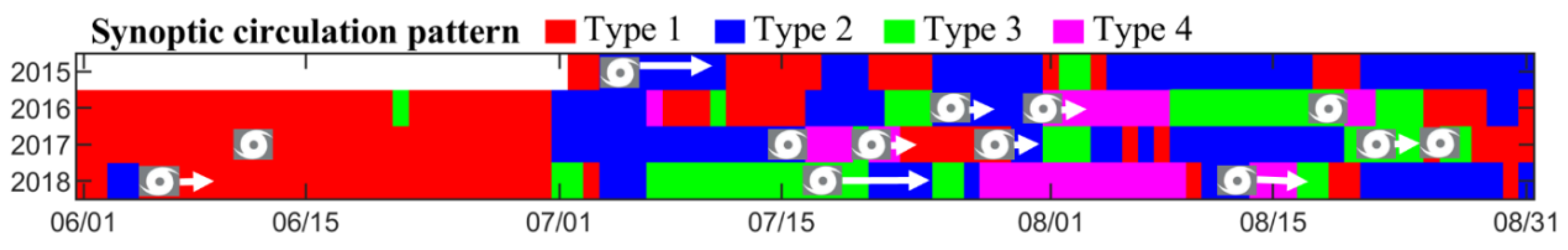
2.2. Classification of Synoptic Types

The T-mode Principal Component Analysis (T-PCA) method is a widely used objective classification method for atmospheric circulation [60,61]; such a method typically does not rely on subjective experience and can process large amounts of data [62]. Things are reversed in T-mode, where the scores describe important spatial patterns and the loadings reflect the amount of their time variant realization. Thus the T-mode seems more appropriate for pattern classification. In addition, T-PCA can display the characteristics of the original circulation field more accurately, without much change owing to the adjustment of the categorized objects, and obtain a more stable spatiotemporal field [62,63]. In this study, the European COST733 weather classification software (http://www.cost733.org, accessed on 17 May 2021) is used for classification and the 500-hPa geopotential height is used as the physical quantity field. The geopotential height is the daily average data with a spatial resolution of 2.5° × 2.5° obtained from NCEP/NCAR reanalysis data. It is considered that the daily circulation pattern is the spatial distribution of the physical quantity field with the largest absolute value of the principal component loadings. The number of circulation types in this article is set to four. Detailed information on the performance of the synoptic classification [64,65] and the determination of the number of classes [66] is provided in the Supplementary Materials (Text S3 and Figure S2).

The overall natural environmental condition of the SCS depends largely on the regional atmospheric circulation system (seasonal monsoon, trade winds, typhoons), whilst these circulation systems in turn influence the formation of the ocean current structure and its spatiotemporal changes [67]. Among these circulation systems, the Northwest Pacific subtropical high (NWPSH; 500-hPa geopotential height field shows significant anticyclonic, and the center is generally accompanied by a descending ) has a greater influence on, or control over, the East Asian summer monsoon, which is most significant in the middle troposphere, and has a more direct and significant impact on the SCS climate [68]. Therefore, to capture the location, shape and intensity of the NWPSH, we set the domain of 0°–50° N and 70°–155° E for the T-PCA analysis, following previous studies [62,63].

Therefore, we use the T-PCA method to objectively classify the large-scale atmospheric circulation of the 500-hPa geopotential height in the summers of 2015–2018, and ultimately obtain four LSCPs related to the movement of the NWPSH (Figure 1):

(1)

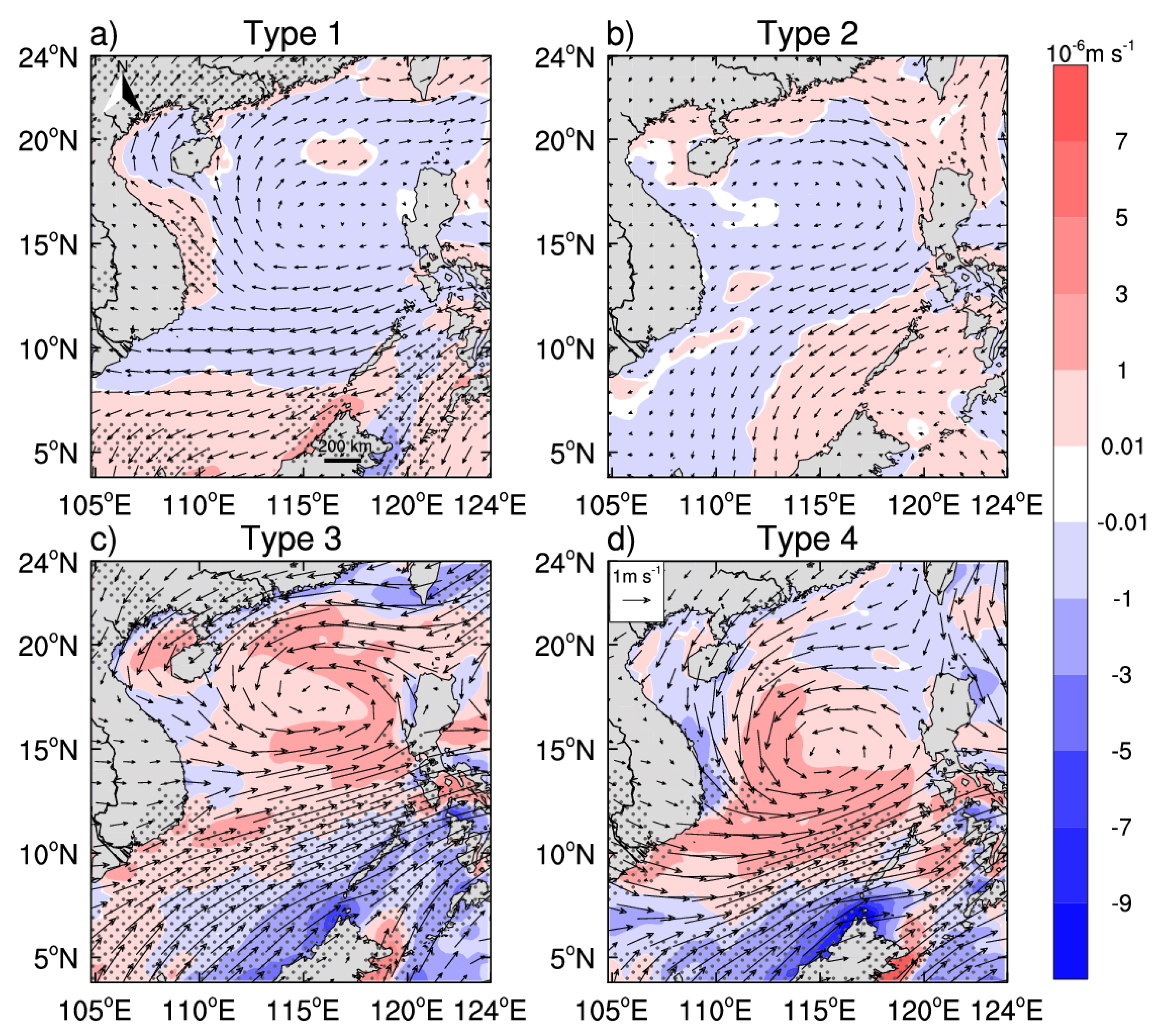
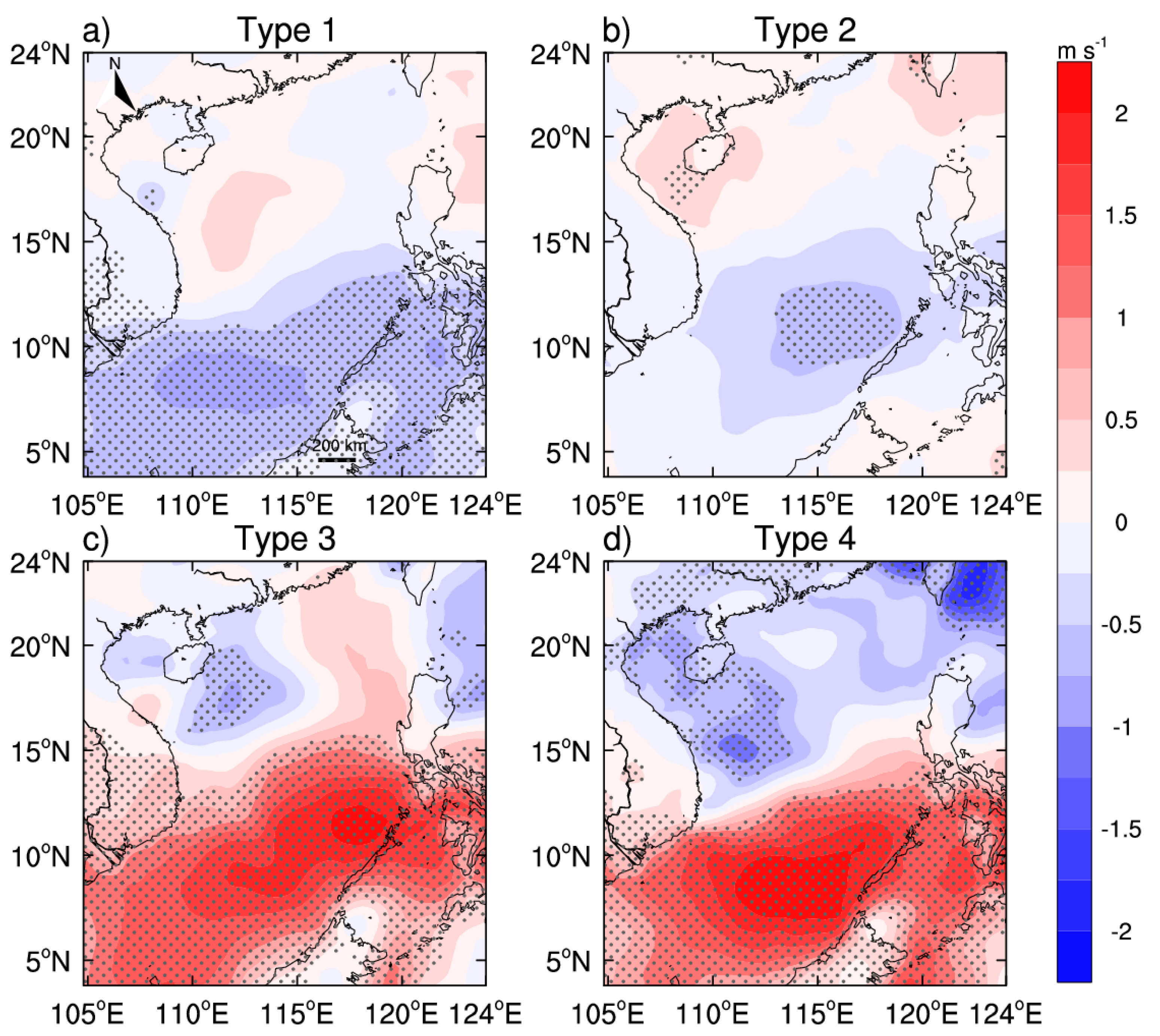
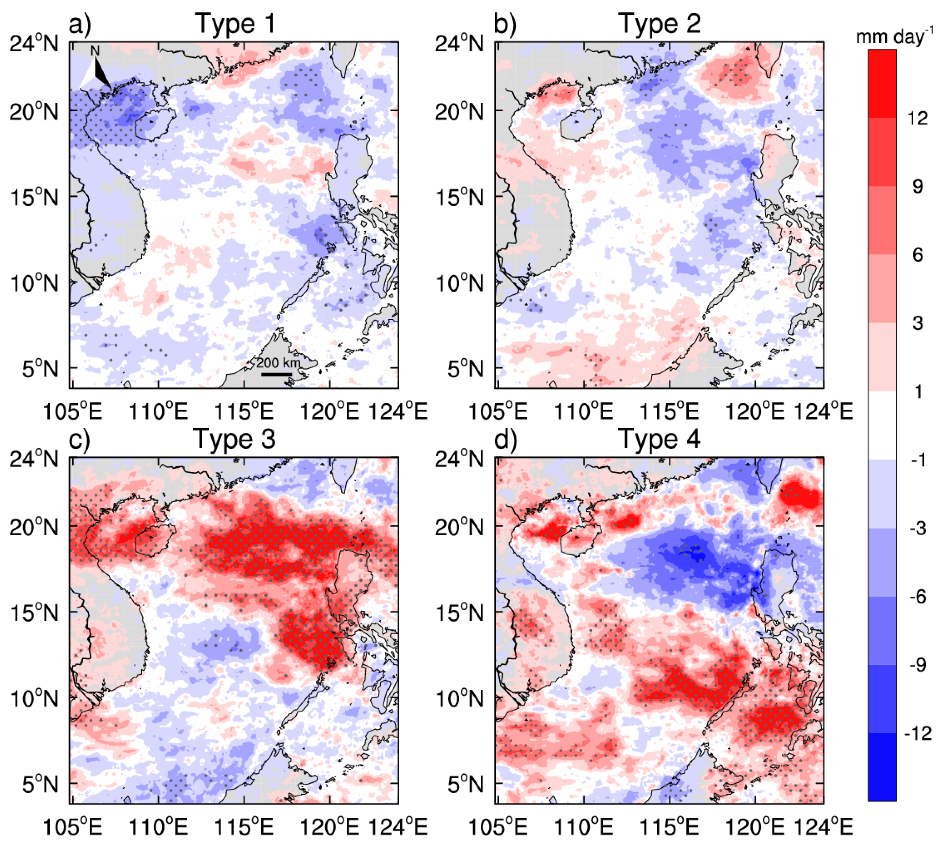
Type 1 is located in the southerly winds on the west side of the NWPSH, which is mainly controlled by the NWPSH. Such conditions are not conducive to ascending motion and precipitation is relatively low.

(2)

In Type 2, the westerly trough deepens meridionally, and the NWPSH advances northward, presenting two anticyclonic centers (Figure 1b). The SCS is located between the Indian low and the NWPSH, and is jointly controlled by both. At the front of the NWPSH bottom forms a southerly wind blowing from the ocean to the mainland.

(3)

While the NWPSH retreats eastward during Type 3, a warm high pressure is formed in North China. The enhancement of low pressure on the west side produces two centers. The SCS is mainly affected by low pressure, and the ascending motion is strong. Southwestward warm and wet airflow makes the rainfall increase.

(4)

In Type 4, the warm high pressure north of the SCS extends westward and advances northward, moving completely to the north side of the SCS. A strong low-pressure center appears in northeastern India, extending eastward to the SCS, at which time the SCS forms southwesterly to southeasterly winds.

From the above analysis, it is concluded that the movement of the NWPSH is bound up with the Indian low and the warm high in northeastern China, which together regulate the weather conditions over the SCS, thereby affecting the changes in the upper ocean environment.

2.3. Significant-Difference Test

To accurately analyze the change in the chl-a concentration under the different LSCPs, the average distributions of chl-a and meteorological variables were calculated for each weather type. Also, the anomaly distributions of these variables were calculated—that is, the differences in the average values of chl-a and meteorological variables under each weather from the average values of the summers of 2015–2018. Then, the variance test or t-test method was used to test the significance at the 0.1 confidence level. From the results it is possible to distinguish any significant differences in the spatial distributions of hydrometeorological variables under the four weather types.

3. Results

3.1. Summer Hydrometeorological Environment Distribution in the SCS

Figure 2 illustrates the hydrological and meteorological distribution characteristics of the SCS during the summers of 2015–2018. It can be seen from the wind speed and wind field (Figure 2a,b) that the SCS is controlled by the southwest monsoon from June to August. The coast of southern Vietnam is the sea area with the highest wind speed and a strong upwelling in the SCS, which is due to the topography of Vietnam. The southwest winds are blocked by the north–south Annam Cordillera mountain range, and the formation of the jet causes Ekman pumping to form an upwelling offshore [22,32,69,70]; whereas, the western boundary currents are superimposed in the southwest SCS so that the offshore upwelling is transported eastwards at about 11.5° N [69,71,72], resulting in an offshore chl-a bloom jet (Figure 2f), where the cold water in the lower layer wells up to result in a lower SST (Figure 2e). The north–south mountain range blocks the southwest wind and causes airflow to descend on the leeward side, making it difficult for precipitation to form; hence, the precipitation here is the lowest in the entire SCS (Figure 2c) and the PAR value is higher (Figure 2d). Correspondingly, the southwest winds blow towards the mountain range, and ascending air is generated on the windward side, which easily forms rainfall. It can be clearly confirmed from Figure 2 that there is a strong rain band [73,74] and weaker PAR with cloud and rain blocking the light in the eastern waters of Luzon Island (Figure 2d).

In addition to the high chl-a concentration near the southern coast of Vietnam, high chl-a concentrations also occur along the coast of Guangdong in China and the Beibuwan Gulf (Annotation in Figure 2a). The coast of Guangdong is located at the estuary of the Pearl River, and the phenomenon of eutrophication in this area is serious. Moreover, dilution caused by the input of waters from the Pearl River has an important impact on chl-a, especially when factoring in the background winds and the runoff [75]. The southwest winds prevailing in summer can be decomposed into eastward coastal winds and northward coastal winds. According to Ekman transport theory, under the action of coastal winds, the diluted water in the Pearl River Estuary and the adjacent shelf area can be transported to the sea in a direction perpendicular to the shoreline. On the other hand, under the action of shoreward winds, the diluted water in the Ekman layer would be transported northeastward along the direction parallel to the shoreline. The wind direction at this time is conducive to the expansion of the diluted waters towards the east of the estuary and the transportation of nutrients to the northern shelf area, which in turn causes phytoplankton proliferation and increased chl-a content [76,77]. As a result, the high chl-a concentration band along the coast of Guangdong in summer is narrow. In summer, the heat capacity of land is smaller than that of seawater, which leads to rapid changes in land temperature. The river water therefore had a higher temperature than seawater. So the sea surface is warmer in the Beibuwan Gulf may be due to the discharge of the Red River, the westerly flow of the Qiongzhou Strait and because the three sides of the northern BBG are adjacent to the land and the shallow sea heats up quickly [78]. Furthermore, the low chl-a concentration of seawater outside the gulf flows into the gulf, limiting the upwelling of nutrients and phytoplankton growth. Based on the above analysis, the high chl-a concentration is only a narrow band along the coast [78,79].

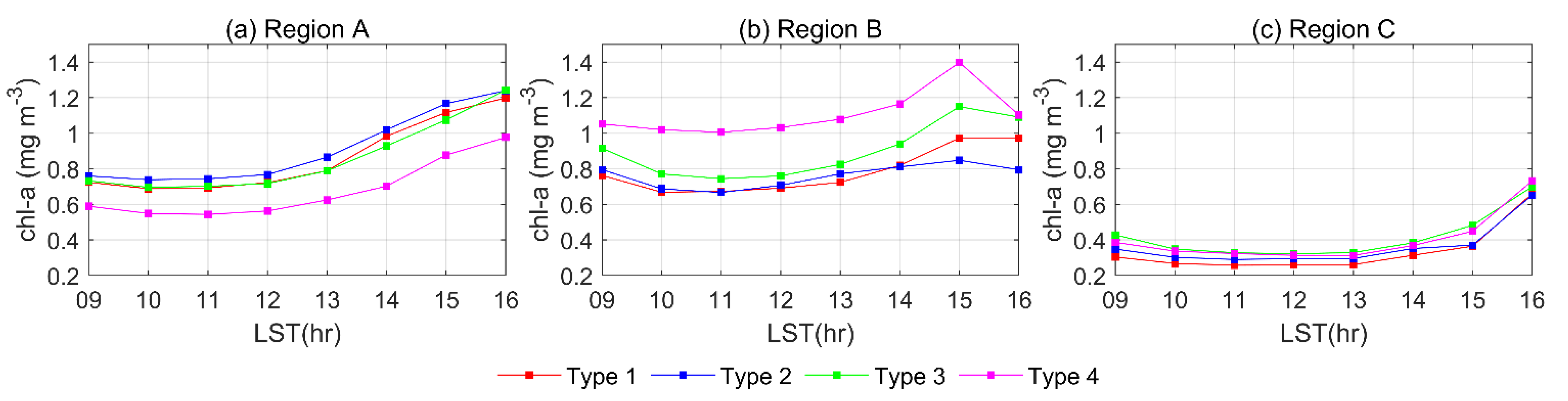
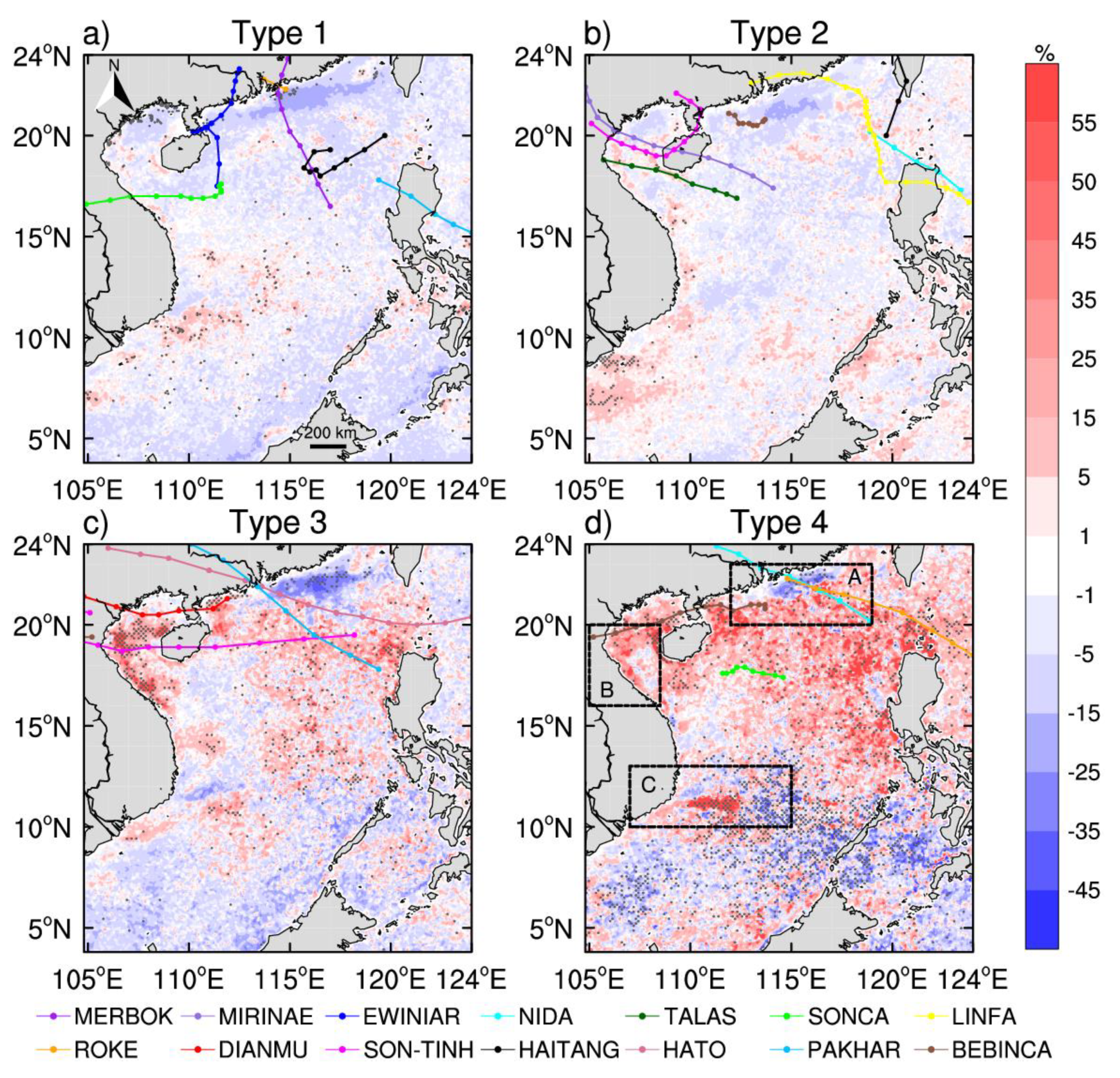
3.2. Disparities of the Biophysical Environment in the SCS under Different LSCPs

To visualize the characteristics of the biophysical environment under the four LSCPs, firstly, the average spatial distribution of chl-a and SST (Figures S3 and S4 in the Supplementary Materials) and the anomalous spatial distribution (Figure 3 and Figure 4) under each LSCP are calculated. The spatial distribution of chl-a characteristics under the four LSCPs in Figure S3 of the SM are roughly similar, showing a gradient change offshore; the chl-a concentration is high near the coast, low in the middle of the basin, and most of the SCS area has a higher chl-a concentration near the west coast than the east coast. In Figure S3 of the SM, Type 1 has a lower chl-a concentration offshore of southern Vietnam. Compared with the other three types, there is no obvious chl-a bloom jet (>0.3 mg m⁻³). For Type 2, the high chl-a concentration zone (>0.3 mg m⁻³) in the Guangdong coastal region has the widest area of coverage. The offshore chl-a bloom jet formed under Type 3 in southern Vietnam is the most obvious. In the last type, Type 4, the high chl-a concentration zone along the coast of Guangdong is the narrowest, and the chl-a concentration in the middle of the SCS is the lowest—a typical desert sea area (<0.1 mg m⁻³).

Comparing the distributions of chl-a anomalies in Figure 3, it can be seen that chl-a is relatively high in most sea areas in Type 2, while in Type 4, it is low except for the Beibuwan Gulf and some offshore waters in southern Vietnam. Positive anomalies occur along the coast of Guangdong in Type 1 and Type 2, while negative anomalies occur in Type 3 and Type 4. In particular, the absolute values of anomalies in Type 2 and Type 4 are larger. The differences in Type 1 and Type 3 in the coast of southern Vietnam and the differences in Type 1 and Type 4 in the southern Beibuwan Gulf are both significant. Based on the above, we selected these three coastal areas (A: Guangdong offshore region; B: Southern Beibuwan Gulf region; C: Southern Vietnam offshore region) to study the daily chl-a changes under the different LSCPs and the reasons for them. In terms of SST, Type 1 has the highest value among the four types (Figure S4 in the Supplementary Materials). Along the southern coast of Vietnam, the range of SST below 29 °C gradually expands from Type 1 to Type 4. Figure 4a shows that SST decreases in the northeastern part of the study area and near the coast of Vietnam (~110° E) in Type 1. Moreover, increased SST characterizes most other sea areas. The SST anomaly distribution of Type 4 (Figure 4d) is completely opposite to that of Type 1. SST rises in the northeast and off the coast of Vietnam, while other sea areas feature more obvious cooling; and both types have a common characteristic insofar as the SST decreases/increases more severely toward the northeast. The distribution pattern of SST anomalies in Type 3 is roughly similar to that of Type 4, with large-scale cooling in the southern waters. In Figure 4c, the negative anomalies in southern Vietnam are the largest, which are lower than the average by more than 0.8 °C. This is consistent with the chl-a bloom jet in Type 3 and is caused by the offshore upwelling that turns the lower layers of nutrient-rich and colder seawater upwards. The abnormal values of SST in Type 2 are mostly small, with a range of ±0.2 °C. Only in the coastal areas of Guangdong is there a significant heating up of the sea surface (Figure 4b).

Figure 5 shows the regional average chl-a changes per hour during 0900–1600 (local standard time, LST = UTC + 8) in the three regions selected in Figure 3d. To exclude the effects of morning and dusk, we choose the period 0900-1600 (LST). The change in chl-a concentration from 0900 to 1300 LST is not obvious, but after 1300 LST a gradual increase begins. This is because, after a day of sufficient sunlight, zooplankton feeding on phytoplankton in the surface ocean at night [80] and enters the deeper ocean during the day, while phytoplankton grows during the day and gradually accumulate chl-a through photosynthesis, giving rise to a high value of chl-a concentration in the evening time. This phenomenon is similar to the findings of Noh et al. [81]. Notably, regions A and C reach their highest values at 1600 LST, while region B reaches its highest value at 1500 LST. Combined with the diurnal chl-a amplitude (maximum chl-a concentration minus minimum chl-a concentration during the period of 0900–1600 each day) under the four LSCPs shown in

Table 1. Diurnal amplitude of the regional chl-a concentration (mg m⁻³) under the four synoptic types.

	Type1	Type2	Type3	Type4
Region A	0.51	0.50	0.55	0.43
Region B	0.30	0.18	0.41	0.39
Region C	0.40	0.36	0.38	0.42

, we can build a picture of the different characteristics in the three regions under the four LSCPs. The Type 4 chl-a concentration in region A is significantly lower than that of the other three types, but the daily amplitude is the most significant (Table 1). The highest daily amplitude is 0.55 mg m⁻³ in Type 3. In region B, the chl-a concentration in Type 3 and Type 4 is higher than that of the other two types, and the daily amplitude is correspondingly larger; the daily amplitude in Type 2 is extremely low, being only 0.18 mg m⁻³. Relatively speaking, the four types of chl-a concentration differences and diurnal variations are weak in region C. The daily amplitude fluctuates at 0.39 ± 0.03 mg m⁻³. In short, the environment of the upper ocean is different under the different LSCP conditions, creating different degrees of daily changes.

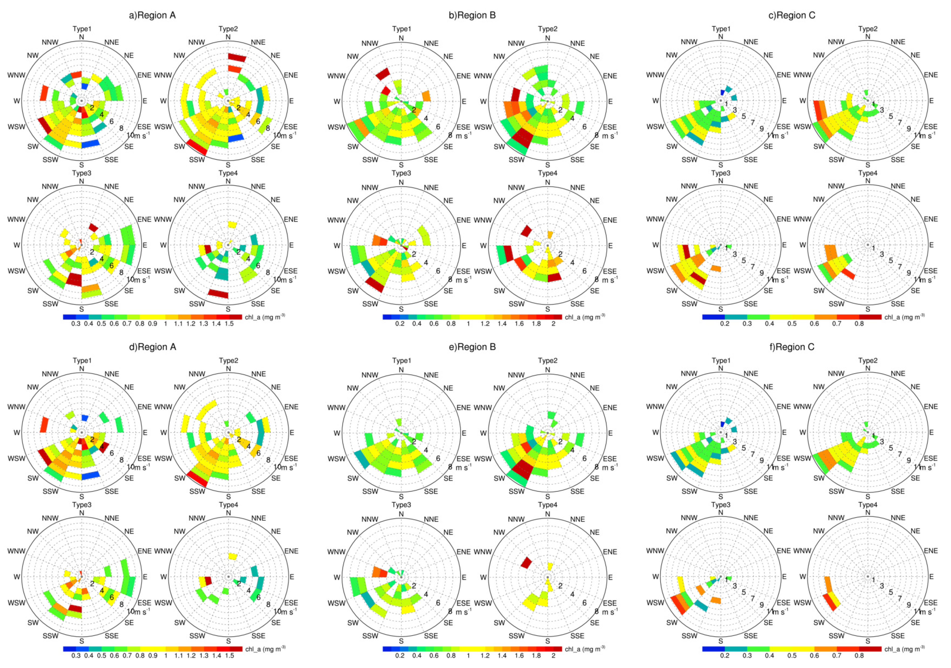
3.3. Potential Drivers of chl-a under Different LSCPs

The wide area and various physicochemical conditions form a vastly different hydrological environment in different areas of the SCS, which affects the stability of the phytoplankton community structure in the local sea area and even the stability of the entire marine ecosystem. Therefore, the local chl-a differences may be caused by different factors.

To explore the potential drivers of chl-a characteristics, we analyzed the average and anomalous distributions of the wind field, upwelling, wind speed, PAR and precipitation under the four LSCPs (Figures S5–S9 in the Supplementary Materials; Figure 6, Figure 7, Figure 8 and Figure 9). At the same time, the influence of Ekman transport in the coastal waters cannot be ignored, and the relationship between Ekman transport and Ekman pumping where chl-a changes drastically in the coastal waters is also considered (Figure S6 in the Supplementary Materials).

The SCS is mainly affected by southwest winds in summer. From the wind vectors (Figure S5 in the Supplementary Materials) and wind speed (Figure S7 in the Supplementary Materials), the sea areas with higher wind speeds are concentrated near southern Vietnam (Region C). Here, the strong southwest wind causes Ekman transport to the southeast (offshore) (Figure S6b,d in the Supplementary Materials), in turn causing the upwelling of deeper seawater near the shore. The greater the offshore Ekman transport value, the stronger the Ekman pumping (Figures S5 and S6 in the Supplementary Materials). Although there is no obvious upwelling in Guangdong (Region A) (Figure S5 in the Supplementary Materials), Figure S6a,c in the Supplementary Materials show that the southwest wind is accompanied by eastward and southward Ekman transport in Region A, which is an offshore Ekman transport perpendicular to the coastline, and the offshore current will trigger a supplementary upwelling and river waters with terrestrial matter transporting to the open sea. Abnormal southwest winds lead to higher chl-a concentration in Region A in Type 1 and Type 2, relative to Type 3 and Type 4 (Figure 3 and Figure 6). The wind field in a semi-enclosed bay like the Beibuwan Gulf (Region B) is affected by the land and the wind direction is various, so the transportation direction of Ekman transport is various. In Type 3 and Type 4, the maximum wind speed in the southern SCS exceeds 10 m s⁻¹ (Figure S7c,d in the Supplementary Materials), and the average increase is more than 1.5 m s⁻¹ (Figure 7c,d). Stronger southwesterly winds cause a strong upwelling in southern Vietnam, about 12 × 10⁻⁶ m s⁻¹ (Figure S5c,d in the Supplementary Materials), bringing low-layer, high-nutrient seawater to the surface. This contributes to phytoplankton growth and forms a chl-a bloom jet, similar to the summer average. In Figure S5c,d of the SM, the divergence direction of the upwelling is more landward under Type 1/Type 2 than Type 3/Type 4 in southern Vietnam. Also, the anomaly distribution of the wind field shows that the two types of wind directions are northeast winds on average (Figure 6a,b), meaning transport by upwelling is not easy, which corresponds to the chl-a bloom jet not being obvious here under Type 1 and Type 2.

Sunlight also affects the SST and chl-a concentration. PAR anomalies show that large areas under Type 1 receive more sunlight, and positive anomalies appear south of 15° N (Figure 8a,b), while Type 3 and 4 show the opposite phenomenon (Figure 8c,d). In contrast, Type 2 also shows negative anomalies to the south of 15° N and positive anomalies north of 15° N, but the anomalies are marginal (Figure 8b). These characteristics are consistent with SST performance. When the PAR value is low, the SST is also low, and vice versa. In addition to the lower PAR, the pattern of the SST cooling to the south of 15° N is different under Type 3 and Type 4. The main reason is that the southern wind field patterns of Type 3 and Type 4 are different (Figure 6c,d). Although the wind anomalies under these two types have formed anomalous cyclonic circulations, the locations of the two cyclonic circulations are different (Figure 6c,d), inducing different effects on different regions of the SCS.

In detail, the anomalous cyclone of Type 3 is mainly located in the northern SCS, so the wind in the south exhibits an increase, while the wind pattern does not change. The prevailing southwesterly winds in southern Vietnam enhance the offshore upwelling and eastward currents, leading to more cooling and nutrient-rich seawater being transported eastward and resultant large-scale sea surface cooling (Figure 4c) and an obvious abnormal chl-a bloom jet here (Figure 3c), which is consistent with previous studies [16,29,34]. In Type 4, the location of the cyclone is in the southern-central SCS, changing the local wind patterns. Due to the change of wind direction in southern Vietnam, the offshore upwelling here is weaker in Type 4 than Type 3, and the chl-a bloom jet is also relatively unobvious (Figure 3d). Therefore, the decrease in SST in Type 4 is mainly controlled by latent heat flux induced by the enhanced wind speed, because strong winds can increase evaporation and exchange at the sea–air interface.

PAR is closely related to cloud cover and precipitation. From Figures S8 and S9 in the Supplementary Materials, PAR and precipitation have a strong negative consistency. When PAR is higher, there is less precipitation. The precipitation anomalies of the SCS for Type 1 and Type 2 are relatively smaller (Figure 9a,b). Correspondingly, the PAR under Type 1 is higher in the southern SCS (Figure 8a), implying that there are clearer skies, less precipitation, lower wind speed and more stable seawater stratification. As a result, the southern SCS shows a warming of surface seawater, with a lower chl-a concentration. In contrast, the changes in various hydrometeorological elements under Type 2 are not obvious, indicating that the weather conditions of Type 2 are stable, which is close to the average distribution in summer. Type 3 has the highest precipitation, since this type of weather is most prevalent in southwesterly winds, and precipitation is more likely to occur on the windward side, such as west of Luzon Island (Figure 9c). Moreover, the above-mentioned Type 3 wind field has anomalous cyclonic circulation relative to the average wind field in the northern SCS (Figure 6c), indicating that there is relatively more convergence and, as a result, more ascending motion, meaning the northern part has heavy rainfall. Differently, a positive rainfall anomaly mainly appears in the southern SCS (Figure 9d), which is also related to the location of southern anomalous cyclonic circulation (Figure 6d).

Overall, the chl-a changes in different regions of the SCS under different LSCPs may be dominated by different meteorological variables. For further quantitative analysis, Figure 10 shows the anomaly percentages of meteorological variables for the three coastal regions, where chl-a changes significantly under the different LSCPs (Figure 3d). Note that, due to precipitation over land and ocean having different effects on chl-a, the coastal precipitation was calculated separately over land and ocean areas. It is also considered that Ekman transport is very important for upwelling in regions A and C.

Table 2. Mean Ekman pumping velocity (×10⁻⁷m s⁻¹) and mean Ekman transport (m² s⁻¹) component vertical to the coastline caused by the wind field under the different synoptic types in Regions A and C.

	Mean Ekman Pumping Velocity/Mean Ekman Transport Component Vertical to the Coastline
	Type 1	Type 2	Type 3	Type 4
Region A	−1.06/−0.20	0.44/−0.23	5.28/0.30	−0.46/0.02
Region C	−2.97/1.74	−0.57/1.72	6.82/2.50	15.33/1.95

shows the regional average of the Ekman pumping velocity and Ekman transport component vertical to the coastline caused by wind stresses in the two regions (Figure 6c). In detail, Region A is the east–west coastline, so Table 2 shows the Ekman transport in the north–south direction (northward is positive), while Region C is the north–south coastline and Table 2 presents the Ekman transport in the east–west direction (eastward is positive). Note that the Ekman pumping velocity in the upwelling center only located in the near shore is larger (Figure S5 in the Supplementary Materials). Meanwhile, because Regions A and C are large, their regional averages for Ekman pumping velocities are smaller. In particular, Ekman transport is larger in the whole of Region C, and thus, the Ekman transport is actually more important to the chl-a jet formation in Region C. In general, the potential drivers of the coastal biophysical environment (chl-a and SST) in the South China Sea can be summarized as follows:

(1) In Type 1, from Figure S10a–c in the Supplementary Materials, it can be seen that Type 1 is the most similar to June, and that the deviation is largely positive. Therefore, Type 1 is the dominant type in June, which is the common influence of the June monsoon circulation and the ocean mesoscale circulation process. The coastal area is also greatly affected by local hydrology [32,82,83]. The wind speed is generally lower in the three coastal regions, and the chl-a concentration is mainly affected by precipitation and upwelling or downwelling. The increase in chl-a in Region A is mainly caused by the increased runoff input from rainfall over the land; in Region B, hydrometeorological variables are generally not conducive to phytoplankton growth. The rainfall over the land is low and the sea temperature is high (more than 30 °C, Figure S4 in the Supplementary Materials). The stratification is relatively stable, leading to less nutrient input. It is clear that precipitation over the ocean has a strong dilution effect in Region C. June is the beginning of the summer SCS circulation. The jet from southern Vietnam to the east has just formed, so it is weaker than the summer average [32,70,83]. For instance, the upwelling in this type is weak, there is a strong eastward (offshore) Ekman transport (Figures S5 and S6 in the Supplementary Materials; Table 2), and the relatively strong sinking is dominant in Region C, which together leads to a low chl-a concentration.

(2) In Type 2, the chl-a concentration in most regions of the SCS is greater than that in June (Figure S10d in the Supplementary Materials), showing the largest deviation relative to June. The southwest wind is strong in Type 2, especially in southern Vietnam where there is strong offshore upwelling and Ekman transport to the southeast. Also, Type 2 exhibits marginal deviation from July and August (Figure S10e,f in the Supplementary Materials), confirming that the strong southwesterly wind in July and August causes the strong eastward jet [32,70,83]. The chl-a in Type 2 is mainly contributed by that in both July and August. The wind speed anomaly percentage value in Region B is 6.38%, but the chl-a concentration still shows a decrease. Because the direction of wind anomalies is offshore (Figure 6b), the accumulation of chl-a is less likely. Also, the increase in precipitation over the ocean is nearly 30%, which offsets some of the input of land runoff. Eventually, there is a slight decrease in chl-a, of about 1.72%. Region A is near the shore, and its summer SST (about 29 °C) is lower than in the open sea (Figure 1e). In the case of Type 2 with weak upwelling and strong Ekman transport (Figures S5 and S6 in the Supplementary Materials and Table 2) in Region A, the SST still increases by 0.4 °C (Figure 4b). The suitable temperature for tropical phytoplankton is between 20 °C and 30 °C, with some phytoplankton bloom with an increase in temperature [84]. There is a stable input of PAR, an increase of SST and, affected by the strong southwesterly winds in July and August, the Ekman advection transport effect caused by the monsoon spreads the nearshore nutrient-rich salt water to offshore and forms upwelling along the coast of Guangdong (Table 2). All of these factors provide a suitable growth environment for some phytoplankton near the shore, thus promoting photosynthesis to increase the concentration of chl-a. Region C is also affected by SST and, combined with the lower precipitation over the ocean, also promotes phytoplankton growth and chl-a accumulation.

(3) In Type 3, Regions A and B receive a lot of rainfall, but the chl-a changes in the two regions are different. Although there is a positive Ekman pumping velocity in Region A, it is affected by precipitation over the ocean, which dilutes the seawater. Also, with the reduction of PAR, photosynthesis is inhibited and the chl-a concentration is reduced. Terrestrial nutrient input induced by rainfall over land plays a major role in the increases of chl-a in region B. The most obvious feature of region C is that the wind speed anomaly percentage exceeds 15%. The strong southwest winds here cause a strong upwelling (Ekman pumping velocity of ~6.82 × 10⁻⁷ m s⁻¹) and strong offshore eastward Ekman transport (1.72 m² s⁻¹) (Table 2, Figures S5 and S6 in the Supplementary Materials), and there is very little precipitation over the ocean, so there is an obvious accumulation of chl-a.

(4) In Type 4, the chl-a concentration changes drastically and is extremely low in region A, at about −29.7%. The wind speed is extremely small, accompanied by downwelling, which inhibits phytoplankton growth. There are many clear-sky weathers in Region B, larger PAR, and suitable SST for increased chl-a. In Region C, there is abundant precipitation over the ocean, which will reduce PAR and dilute nutrients, inducing chl-a decrease. Meanwhile, strong winds cause strong upwelling (Ekman pumping velocity of 15.33 × 10⁻⁷ m s⁻¹), and strong Ekman transport (1.95 m² s⁻¹) (Table 2, Figures S5 and S6 in the Supplementary Materials) and the large amount of precipitation over land can induce strong terrestrial nutrient inputs into coastal waters, resulting in positive anomalies of chl-a.

4. Discussion

4.1. Contribution of Typhoons under Different LSCPs

Due to the special geographic location and complex surrounding terrain of the SCS, the multiscale ocean dynamic processes of its upper circulation will be affected by various external factors [85,86,87]; one of the most important factors is typhoons. On average, 10.3 typhoons affect the SCS every year, occurring frequently from July to September, including typhoons moving westward from the Northwest Pacific and those generated in the southern part of the SCS [88,89,90]. Previous studies have clarified that typhoons can cause local vertical mixing or entrainment and upwelling in the SCS, which can bring deeper, nutrient-rich water from the subsurface to the surface light-transmitting layer, thereby promoting an increase in the chl-a concentration and oceanic phytoplankton/primary productivity [18,66,91,92,93,94,95,96,97,98,99]. To explore the contribution of typhoons, an extreme synoptic weather pattern, to each LSCP, we removed the samples during typhoon events and recalculated the chl-a pattern in each LSCP using the following steps.

First, the number of typhoons and their dates of impact during the study period were counted (

Table 3. Typhoon statistics under the four synoptic types in 2015 (July, August) and 2016–2018 (June, July, August).

	Type 1	Type 2	Type 3	Type 4
Typhoon number	6	7	5	4
Typhoon affected days *	40	27	23	20
Percentage of days affected by typhoons (%)	29.4	23.1	44.2	62.5

* The number of days in a week after typhoon transit and typhoon dissipation.

and Table S1, Figure 11). The total sample days and the days for each type from July to August after removing the typhoon impact days can be referred to in Tables S2 and S3 of the SM. As can be seen, although the numbers of typhoons in Type 1 and Type 2 are larger, the proportion of days affected by typhoons is low, less than 30%. Type 4 is the most affected by typhoons, with 62.5% of the sample days being affected by typhoons. Figure 11 shows the daily changes of each weather type in the summers of 2015–2018; the start and end time of each typhoon are also marked in the figure. Notably, Type 1 mainly appears in June, while Type 2, Type 3 and Type 4 mainly appear in July and August. This is because the NWSPH moves southwest mainly in June, and gradually moves northwards from July to August [66,85].

Secondly, using all sample days under each type minus the sample days without typhoon influence, and then dividing by the sample days without typhoon influence, the effect of typhoons on chl-a in the four LSCPs was obtained (Figure 12). Figure 12 also shows the paths of typhoons under each LSCP. During the study period, typhoons mainly pass through the northern part of the SCS. In Type 1 and Type 2, the contribution of typhoons is smaller, and most chl-a concentration fractions in the northern SCS are within ±15%. Yet, the contributions of typhoons in Type 3 and Type 4 are more obvious, and the chl-a concentration is higher overall in the northern SCS during Type 4, at approximately 15–50%. Therefore, Type 3 and Type 4 are more likely to be short-term disturbances and are more affected by typhoons, while Type 1 and Type 2 are part of the annual South China Sea monsoon cycle (Figure S10 in the Supplementary Materials and Figure 11; Tables S2 and S3 in the Supplementary Materials). There is one common point in the four types of LSCP. There are negative values in coastal Guangdong, where the suspended sediment content is high [100], indicating that typhoons always make a negative contribution there. This phenomenon is similar to the findings of a previous study [101]. After the passage of typhoons, the upper-ocean hydrologic environment is disturbed; that is, suspended sediment floats upwards and the concentration of suspended sediment in the sea surface layer increases. Subsequently, the transparency of seawater reduces, lowering the efficiency of photosynthesis.

4.2. Roles of Various Wind Vectors under Different LSCPs

According to previous studies [99,102], typhoon wind directions are varied, which may cause different chl-a changes in different sea areas. The chl-a anomaly was also applied to the samples with typhoons removed (Figure S11 in the Supplementary Materials). In contrast, the chl-a changes are more significant without the influence of typhoons, and the negative anomalies cover most of the range. This feature is generally consistent with the positive contribution of typhoons to chl-a. It can also be concluded that the previous three regions have significant differences under different LSCPs, and that the relationship between the chl-a and wind in these regions can be demonstrated. Figure 13a–c show the chl-a concentration of different types for all sample days, while Figure 13d–f show the chl-a concentration of different types without typhoon days. For all sample days, the wind direction of Region A is blocked by land, especially in Type 1 and Type 2. Regions B and C are controlled by southwest winds, and chl-a is lower in Type 1. Chl-a is higher, but the wind speed is low during Type 4 in Region B. In contrast, high wind speeds correspond to a higher chl-a concentration during Type 2 in Region C. All three regions show that the high chl-a concentration is controlled by strong wind (>4 m s⁻¹); and under the same wind direction, the greater the wind speed, the higher the chl-a concentration. Nevertheless, after removing the typhoon samples, some samples of strong north winds with high chl-a values in Regions A and B are eliminated (Figure 13d,e), which means that strong northerly winds will cause elevated chl-a. These strong north winds are brought by typhoons. Comparing the three sea regions, without the influence of typhoons, the regional sea surface wind directions are more concentrated, being mainly influenced by the southwest monsoon. Samples with high chl-a concentration under the control of strong southward winds are also affected. It is possible that typhoons aggravate the effect of the southwest monsoon and increase the chl-a concentration.

In summary, typhoon wind pump mainly contribute to the increase in chl-a concentration in most regions under strong winds or northerly winds. In contrast, for the coastal area of Guangdong, compared with the typhoon contribution shown in Figure 12, the chl-a concentration mainly decreases on some typhoon-passing days, due to the weakened efficiency of photosynthesis under the enhancement of suspended sediment induced by typhoons.

5. Conclusions

In this ppaper, we used the T-PCA objective classification method to divide the 500-hPa atmospheric circulation in the summers of 2015–2018 into four LSCPs. We found that these four types are closely correlated to the spatiotemporal changes of the NWPSH. Using a variety of satellite datasets, we analyzed the spatiotemporal distribution of chl-a concentration and SST in the SCS under the four types, and discussed the potential causes of changes in chl-a concentration.

Chl-a anomalies in the SCS differ significantly under the four types, especially in coastal waters. Furthermore, these differences are mainly modulated by different local meteorological variables (such as the wind direction, wind speed, PAR and precipitation) related to the movement of the NWPSH, together with local marine hydrologic and topographic environmental factors (e.g., Ekman pumping and transport, SST, nearshore and offshore areas). In particular, under the LSCP controlled by the strong southwest monsoon, the high chl-a concentration jet in the offshore area of southern Vietnam is more significant owing to strong Ekman transport and Ekman pumping. In addition, precipitation over land and ocean has opposite effects on the regulation of chl-a changes in coastal areas. That is, the precipitation over land will transport more terrestrial material to the near shore, which is beneficial to an increase in chl-a, while that over the ocean will reduce PAR and the chl-a concentration.

In our study of diurnal variations, three coastal regions were selected: Guangdong offshore region (A), southern Beibuwan Gulf region (B) and southern Vietnam offshore region (C). Generally, chl-a begins to increase gradually at 1300 LST, and high values erupt in the late afternoon in these three regions. In contrast, Region B reaches its maximum at 1500 LST, whereas the other two regions reach theirs at 1600 LST. The Type-4 diurnal variation in Region A is significantly lower than that of the other types, and the chl-a concentration during Type 3 and Type 4 in Region B is higher. All these results indicate that the chl-a diurnal amplitudes change under different LSCPs.

Additionally, the impact of typhoon wind pump on chl-a in the SCS should not be ignored; such effects are more prominent under Type 3 and Type 4. Typhoons contribute positively to the primary productivity in most of the SCS, except for coastal Guangdong, where chl-a decreases to varying degrees in the four types. This is due to the disturbance of the upper ocean after a typhoon; that is, the seawater with abundant suspended sediment [100] becomes turbid in coastal Guangdong, reducing the photosynthetic efficiency and inhibiting phytoplankton growth [101]). Judging from the relationship between local wind speed and chl-a, typhoons still contribute positively. The strong wind speed brought by a typhoon corresponds to a high chl-a concentration.

In summary, the LSCPs identified by T-PCA in this study are closely linked to the location of the development of NWPSH and the surrounding weather system (Figure 1; [72,99,103]), jointly affecting the hydrological and meteorological environment of the SCS. Our findings show that Type 1 and Type 2 are part of the annual cycle of the SCS monsoon, while Type 3 and Type 4 are more likely to be short-term disturbances and are more affected by typhoons. This results in different chl-a changes via the modulation of local meteorological as well as hydrological conditions, regulating primary productivity in local regions. In particular, the SST front generated by the upwelling of cold water rich in nutrients (phytoplankton) corresponds to an area where pelagic fish are highly concentrated [104,105]. The present work deepens our understanding of the complex features of the ecological environment on multiple temporal scales in the upper layer of the SCS. In general, our findings have important implications for wind pump impact upper ocean and marine environmental monitoring, disaster monitoring and fishery management in offshore waters.

References

1. Ryther, J.H.; Yentsch, C.S. The estimation of phytoplankton production in the ocean from chlorophyll and light data. Limnol. Oceanogr. 1957, 2, 281–286. [Google Scholar] [CrossRef]
2. Bai, Y.; Pan, D.; Guan, W.; He, X. Ocean primary production estimate of China Sea by hy-1a/cocts. Proc. SPIE 2005, 597704. [Google Scholar] [CrossRef]
3. Lomas, M.W.; Moran, S.B.; Casey, J.R.; Bell, D.W.; Tiahlo, M.; Whitefield, J.; Kelly, R.P.; Mathis, J.T.; Cokelet, E.D. Spatial and seasonal variability of primary production on the Eastern Bering Sea shelf. Deep Sea Res. Part II 2012, 65, 126–140. [Google Scholar] [CrossRef]
4. Liu, Y.; Tang, D.; Evgeny, M. Chlorophyll Concentration Response to the Typhoon Wind-Pump Induced Upper Ocean Processes Considering Air–Sea Heat Exchange. Remote Sens. 2019, 11, 1825. [Google Scholar] [CrossRef] [Green Version]
5. Hays, G.C.; Richardson, A.J.; Robinson, C. Climate change and marine plankton. Trends Ecol. Evol. 2005, 20, 337–344. [Google Scholar] [CrossRef]
6. Lin, I.I. Typhoon-induced phytoplankton blooms and primary productivity increase in the western North Pacific subtropical ocean. J. Geophys. Res. 2012, 117. [Google Scholar] [CrossRef]
7. Tang, D.; Kawamura, H.; Van Dien, T.; Lee, M. Offshore phytoplankton biomass increase and its oceanographic causes in the South China Sea. Mar. Ecol. Prog. Ser. 2004, 268, 31–41. [Google Scholar] [CrossRef]
8. Sun, L.; Yang, Y.; Xian, T.; Lu, Z.; Fu, Y. Strong enhancement of chlorophyll a concentration by a weak typhoon. Mar. Ecol. Prog. Ser. 2010, 39–50. [Google Scholar] [CrossRef]
9. Waliser, D.E.; Murtugudde, R.; Strutton, P.; Li, J.L. Subseasonal organization of ocean chlorophyll: Prospects for prediction based on the Madden-Julian Oscillation. Geophys. Res. Lett. 2005, 32, L23602. [Google Scholar] [CrossRef]
10. Liu, S.; Tang, D.; Yan, H.; Ning, G.; Liu, C.; Yang, Y. Potential Associations between Low-Level Jets and Intraseasonal and Semi-Diurnal Variations in Coastal Chlorophyll—A over the Beibuwan Gulf, South China Sea. Remote Sens. 2021, 13, 1194. [Google Scholar] [CrossRef]
11. Cham, D.D.; Son, N.T.; Minh, N.Q.; Thanh, N.T.; Dung, T.T. An analysis of shoreline changes using combined multitemporal remote sensing and digital evaluation model. Civ. Eng. J. 2020, 6, 1–10. [Google Scholar] [CrossRef]
12. Hu, S.; Zhou, W.; Wang, G.; Cao, W.; Xu, Z.; Liu, H.; Wu, G.; Zhao, W. Comparison of Satellite-Derived Phytoplankton Size Classes Using In-Situ Measurements in the South China Sea. Remote Sens. 2018, 10, 526. [Google Scholar] [CrossRef] [Green Version]
13. Kutser, T. Quantitative detection of chlorophyll in cyanobacterial blooms by satellite remote sensing. Limnol. Oceanogr. 2004, 49, 2179–2189. [Google Scholar] [CrossRef]
14. Solanki, H.U.; Mankodi, P.C.; Dwivedi, R.M.; Nayak, S. Satellite observations of main oceanographic processes to identify ecological associations in the Northern Arabian Sea for fishery resources exploration. Hydrobiologia 2008, 612, 269–279. [Google Scholar] [CrossRef]
15. Gholami, D.M.; Baharlouii, M. Monitoring long-term mangrove shoreline changes along the northern coasts of the Persian Gulf and the Oman Sea. Emerg. Sci. J. 2019, 3, 88–100. [Google Scholar] [CrossRef] [Green Version]
16. Warren, M.A.; Quartly, G.D.; Shutler, J.D.; Miller, P.I.; Yoshikawa, Y. Estimation of Ocean Surface Currents from Maximum Cross Correlation applied to GOCI geostationary satellite remote sensing data over the Tsushima (Korea) Straits. J. Geophys. Res. Oceans 2016, 121, 6993–7009. [Google Scholar] [CrossRef] [Green Version]
17. Ciani, D.; Charles, E.; Nardelli, B.; Rio, M.H.; Santoleri, R. Ocean currents reconstruction from a combination of altimeter and ocean colour data: A feasibility study. Remote Sens. 2021, 13, 2389. [Google Scholar] [CrossRef]
18. Liu, Y.; Tang, D.; Tang, S.; Evgeny, M.; Liang, W.; Sui, Y. A case study of Chlorophyll a response to tropical cyclone Wind Pump considering Kuroshio invasion and air-sea heat exchange. Sci. Total Environ. 2020, 741. [Google Scholar] [CrossRef] [PubMed]
19. Palacz, A.P.; Xue, H.; Armbrecht, C.; Zhang, C.; Chai, F. Seasonal and inter-annual changes in the surface chlorophyll of the South China Sea. J. Geophys. Res. 2011, 116. [Google Scholar] [CrossRef]
20. Vantrepotte, V.; Mélin, F. Inter-annual variations in the seawifs global chlorophyll a concentration (1997–2007). Deep Sea Res. Part I 2011, 58, 429–441. [Google Scholar] [CrossRef]
21. Gong, G.C.; Liu, K.K.; Liu, C.T.; Pai, S.C. The chemical hydrography of the South China Sea west of Luzon and a comparison with the West Philippine Sea. Terr. Atmos. Ocean. Sci. 1993, 3, 587–602. Available online: http://140.112.114.62/handle/246246/114465 (accessed on 12 April 2021). [CrossRef]
22. Liang, W.; Tang, D.; Luo, X. Phytoplankton size structure in the western South China Sea under the influence of a ‘jet-eddy system’. J. Mar. Syst. 2018, 187, 82–95. [Google Scholar] [CrossRef]
23. Pan, G.; Chai, F.; Tang, D.L.; Wang, D.X. Marine phytoplankton biomass responses to typhoon events in the South China Sea based on physical-biogeochemical model. Ecol. Model. 2017, 356, 38–47. [Google Scholar] [CrossRef]
24. Siswanto, E.; Ye, H.J.; Yamazaki, D.; Tang, D.L. Detailed spatiotemporal impacts of El Niño on phytoplankton biomass in the South China Sea. J. Geophys. Res. Oceans 2017, 122, 2709–2723. [Google Scholar] [CrossRef]
25. Wang, J.J.; Tang, D.L.; Sui, Y. Winter phytoplankton bloom induced by subsurface upwelling and mixed layer entrainment southwest of Luzon strait. J. Marine Syst. 2010, 83, 141–149. [Google Scholar] [CrossRef]
26. Yan, H.; Liu, C.C.; An, Z.S.; Yang, W.; Yang, Y.J.; Huang, P.; Qiu, S.C.; Zhou, P.C.; Zhao, N.Y.; Fei, H.B.; et al. Extreme weather events recorded by daily to hourly resolution biogeochemical proxies of marine giant clam shells. Proc. Natl. Acad. Sci. USA 2020, 117, 201916784. [Google Scholar] [CrossRef] [Green Version]
27. Ye, H.J.; Sheng, J.Y.; Tang, D.L.; Siswanto, E.; Kalhoro, M.A.; Sui, Y. Storm-induced changes in pco2 at the sea surface over the northern south china sea during typhoon wutip. J. Geophys. Res. Oceans 2017, 122, 4761–4778. [Google Scholar] [CrossRef]
28. He, L.; Yin, K.; Yuan, X.; Li, D.; Zhang, D.; Harrison, P. Spatial distribution of viruses, bacteria and chlorophyll in the northern South China Sea. Aquat. Microb. Ecol. 2009, 54, 153–162. [Google Scholar] [CrossRef] [Green Version]
29. Nguyen, T.; Hoang, T.D. Studies on phytoplankton pigments: Chlorophyll, total carotenoids and degradation products in Vietnamese waters. In Proceedings of the Fourth Technical Seminar on Marine Fishery Resources Survey in the South China Sea, Area IV: Vietnamese Waters, Bangkok, Thailand, 18–20 September 2000; pp. 233–250. [Google Scholar]
30. Wu, M.; Wang, Y.; Wang, Y.; Yin, J.; Dong, J.; Jiang, Z.; Sun, F. Scenarios of nutrient alterations and responses of phytoplankton in a changing Daya Bay, South China Sea. J. Mar. Syst. 2017, 165, 1–12. [Google Scholar] [CrossRef]
31. Tang, D.; Kawamura, H.; Doannhu, H.; Takahashi, W. Remote sensing oceanography of a harmful algal bloom off the coast of southeastern Vietnam. J. Geophys. Res. 2004, 109. [Google Scholar] [CrossRef]
32. Xie, S.P.; Xie, Q.; Wang, D.; Liu, W.T. Summer upwelling in the South China Sea and its role in regional climate variations. J. Geophys. Res. 2003, 108. [Google Scholar] [CrossRef] [Green Version]
33. Wang, J.; Tang, D.L. Phytoplankton patchiness during spring intermonsoon in western coast of South China Sea. Deep Sea Res. Part II 2014, 101, 120–128. [Google Scholar] [CrossRef]
34. Liu, H.; Song, X.; Huang, L.; Tan, Y.; Zhang, J. Phytoplankton biomass and production in northern South China Sea during summer: Influenced by Pearl River discharge and coastal upwelling. Acta Ecol. Sin. 2011, 31, 133–136. [Google Scholar] [CrossRef]
35. Song, X.; Lai, Z.; Ji, R.; Chen, C.; Zhang, J.; Huang, L.; Yin, J.; Wang, Y.; Lian, S.; Zhu, X. Summertime primary production in northwest South China Sea: Interaction of coastal eddy, upwelling and biological processes. Cont. Shelf Res. 2012, 48, 110–121. [Google Scholar] [CrossRef]
36. Yang, Y.J.; Xian, T.; Sun, L.; Fu, Y. Summer Monsoon Impacts on Chlorophyll-a Concentration in the Middle of the South China Sea: Climatological Mean and Annual Variability. Atmos. Ocean. Sci. Lett. 2012, 5, 15–19. [Google Scholar] [CrossRef]
37. Liu, F.; Chen, C.; Zhan, H. Decadal variability of chlorophyll a in the South China Sea: A possible mechanism. Chin. J. Oceanol. Limn. 2012, 30, 1054–1062. [Google Scholar] [CrossRef] [Green Version]
38. Kuo, N.; Ho, C.; Lo, Y.; Huang, S.; Chang, L. Analysis of chlorophyll-a concentration around the South China Sea from ocean color images. In Proceedings of the OCEANS 2009-EUROPE, Bremen, Germany, 11–14 May 2009. [Google Scholar] [CrossRef]
39. Liu, K.; Wang, L.; Dai, M.; Tseng, C.; Yang, Y.; Sui, C.; Oey, L.; Tseng, K.; Huang, S. Inter-annual variation of chlorophyll in the northern South China Sea observed at the SEATS Station and its asymmetric responses to climate oscillation. Biogeosciences 2013, 10, 7449–7462. [Google Scholar] [CrossRef] [Green Version]
40. Lin, J.; Tang, D.; Alpers, W.; Wang, S. Response of dissolved oxygen and related marine ecological parameters to a tropical cyclone in the South China Sea. Adv. Space Res. 2014, 53, 1081–1091. [Google Scholar] [CrossRef]
41. Shang, S.; Li, L.; Sun, F.; Wu, J.; Hu, C.; Chen, D.; Ningm, X.; Qiu, Y.; Zhang, C.; Shang, S. Changes of temperature and bio-optical properties in the South China Sea in response to Typhoon Lingling, 2001. Geophys. Res. Lett. 2008, 35. [Google Scholar] [CrossRef] [Green Version]
42. Ye, H.J.; Sui, Y.; Tang, D.L.; Afanasyev, Y.D. A subsurface chlorophyll a bloom induced by typhoon in the South China Sea. J. Mar. Syst. 2013, 128, 138–145. [Google Scholar] [CrossRef]
43. Yue, X.; Zhang, B.; Liu, G.; Li, X.; Zhang, H.; He, Y. Upper Ocean Response to Typhoon Kalmaegi and Sarika in the South China Sea from Multiple-Satellite Observations and Numerical Simulations. Remote Sens. 2018, 10, 348. [Google Scholar] [CrossRef] [Green Version]
44. Zhao, H.; Tang, D.; Wang, Y. Comparison of phytoplankton blooms triggered by two typhoons with different intensities and translation speeds in the South China Sea. Mar. Ecol. Prog. Ser. 2008, 365, 57–65. [Google Scholar] [CrossRef] [Green Version]
45. Ramos, A.M.; Pires, A.C.; Sousa, P.; Trigo, R.M. The use of circulation weather types to predict upwelling activity along the western Iberian Peninsula coast. Cont. Shelf Res. 2013, 69, 38–51. [Google Scholar] [CrossRef]
46. Moron, V.; Gouirand, I.; Taylor, M. Weather types across the Caribbean basin and their relationship with rainfall and sea surface temperature. Clim. Dyn. 2016, 47, 601–621. [Google Scholar] [CrossRef]
47. Picado, A.; Lorenzo, M.N.; Alvarez, I.; Decastro, M.; Vaz, N.; Dias, J.M. Upwelling and Chl-a spatiotemporal variability along the Galician coast: Dependence on circulation weather types. Int. J. Climatol. 2016, 36, 3280–3296. [Google Scholar] [CrossRef]
48. Murakami, H. Ocean color estimation by Himawari-8/AHI. Proc. SPIE 2016, 9878, 987810. [Google Scholar] [CrossRef]
49. Liu, X.; Wang, M. Analysis of ocean diurnal variations from the Korean Geostationary Ocean Color Imager measurements using the DINEOF method. Estuar. Coast. Shelf Sci. 2016, 180, 230–241. [Google Scholar] [CrossRef]
50. Wang, M.; Ahn, J.; Jiang, L.; Shi, W.; Son, S.; Park, Y.; Ryu, J. Ocean color products from the Korean Geostationary Ocean Color Imager (GOCI). Opt. Express 2013, 21, 3835–3849. [Google Scholar] [CrossRef]
51. Ryu, J.; Han, H.; Cho, S.; Park, Y.; Ahn, Y. Overview of geostationary ocean color imager (GOCI) and GOCI data processing system (GDPS). Ocean Sci. J. 2012, 47, 223–233. [Google Scholar] [CrossRef]
52. Iwasaki, S. Daily Variation of Chlorophyll-A Concentration Increased by Typhoon Activity. Remote Sens. 2020, 12, 1259. [Google Scholar] [CrossRef] [Green Version]
53. Price, J.F. Upper ocean response to a hurricane. J. Phys. Oceanogr. 1981, 11, 153–175. [Google Scholar] [CrossRef] [Green Version]
54. Jaimes, B.; Shay, L.K. Enhanced wind-driven downwelling flow in warm oceanic eddy features during the intensification of Tropical Cyclone Isaac (2012): Observations and theory. J. Phys. Oceanogr. 2015, 45, 1667–1689. [Google Scholar] [CrossRef]
55. Powell, M.D.; Vickery, P.J.; Reinhold, T.A. Reduced drag coefficient for high wind speeds in tropical cyclones. Nature 2003, 422, 279–283. [Google Scholar] [CrossRef] [PubMed]
56. Chereskin, T.K.; Price, J.F. Ekman Transport and Pumping. In Encyclopedia of Ocean Sciences, 1st ed.; Steele, J.H., Ed.; Academic Press: Cambridge, MA, USA, 2001; pp. 809–815. [Google Scholar] [CrossRef]
57. Abdulrazzaq, Z.T.; Hasan, R.H.; Aziz, N.A. Integrated TRMM Data and Standardized Precipitation Index to Monitor the Meteorological Drought. Civ. Eng. J. 2019, 5, 1590–1598. [Google Scholar] [CrossRef] [Green Version]
58. Kuriqi, A. Assessment and quantification of meteorological data for implementation of weather radar in mountainous regions. Mausam 2016, 67, 789–802. [Google Scholar]
59. Yang, Y.J.; Wang, H.; Chen, F.J.; Zheng, X.Y.; Fu, Y.F.; Zhou, S.X. TRMM-based Optical and Microphysical Features of Precipitating Clouds in Summer over the Yangtze-Huaihe River Valley, China. Pure Appl. Geophys. 2019, 176, 357–370. [Google Scholar] [CrossRef]
60. Compagnucci, R.H.; Richman, M.B. Can principal component analysis provide atmospheric circulation or teleconnection patterns? Int. J. Climatol. 2008, 28, 703–726. [Google Scholar] [CrossRef]
61. Huth, R. An example of using obliquely rotated principal components to detect circulation types over Europe. Meteorol. Ztschrift 1993, 2, 285–293. [Google Scholar] [CrossRef]
62. Zong, L.; Yang, Y.J.; Wang, H.; Ning, G.C.; Li, Y.B.; Gao, Z.Q.; Liu, C.; Wang, L.L. Synoptic drivers of co-occurring surface ozone and PM2.5 pollution during summertime ineastern China. Atmos. Chem. Phys. 2021, 21, 9105–9124. [Google Scholar] [CrossRef]
63. Yang, Y.J.; Wang, R.; Chen, F.J.; Liu, C.; Bi, X.Y.; Huang, M. Synoptic weather patterns modulate the frequency, type and vertical structure of summer precipitation over Eastern China: A perspective from GPM observations. Atmos. Res. 2020, 05342. [Google Scholar] [CrossRef]
64. Hoffmann, P.; Heinke SchlüNzen, K. Weather pattern classification to represent the urban heat island in present and future climate. J. Appl. Meteorol. Clim. 2013, 52, 2699–2714. [Google Scholar] [CrossRef]
65. Philipp, A.; Beck, C.; Esteban, P.; Krennert, T.; Lochbihler, K.; Spyros, P.; Pianko-kluczynska, K.; Post, P.; Alvarez, R.; Spekat, A.; et al. Cost733 User Guide; University of Augsburg: Augsburg, Germany, 2014. [Google Scholar]
66. Ning, G.; Yim, S.H.L.; Wang, S.; Duan, B.; Nie, C.; Yang, X.; Wang, J.; Shang, K. Synergistic effects of synoptic weather patterns and topography on air quality: A case of the Sichuan Basin of China. Clim. Dynam. 2019, 53, 6729–6744. [Google Scholar] [CrossRef]
67. Vlasova, G.A.; Demenok, M.N.; Xuan, N.B.; Long, B.H. The role of atmospheric circulation in spatial and temporal variations in the structure of currents in the western South China Sea. Izv. Atmos. Ocean. Phys. 2016, 52, 317–327. [Google Scholar] [CrossRef]
68. He, X.Z.; Gong, D.Y. Interdecadal change in Western Pacific Subtropical High and climatic effects. J. Geogr. Sci. 2002, 12, 202–209. [Google Scholar] [CrossRef]
69. Dippner, J.W.; Nguyen, K.V.; Hein, H.; Ohde, T.; Loick, N. Monsoon-induced upwelling off the Vietnamese coast. Ocean Dynam. 2007, 57, 46–62. [Google Scholar] [CrossRef]
70. Wang, G.; Chen, D.; Su, J. Generation and life cycle of the dipole in the South China. Sea summer circulation. J. Geophys. Res. 2006, 111. [Google Scholar] [CrossRef] [Green Version]
71. Chen, C.; Lai, Z.; Beardsley, R.C.; Xu, Q.; Lin, H.; Viet, N.T. Current separation and upwelling over the southeast shelf of Vietnam in the South China Sea. J. Geophys. Res. 2012, 117. [Google Scholar] [CrossRef] [Green Version]
72. Wang, D.; Wang, Q.; Cai, S.; Cai, S.; Shang, X.; Peng, S.; Shu, Y.; Xiao, J.; Xie, X.H.; Zhang, Z.; et al. Advances in research of the mid-deep South China Sea circulation. Sci. China Earth Sci. 2019, 62, 1992–2004. [Google Scholar] [CrossRef]
73. Xu, H.; Xie, S.P.; Wang, Y.; Zhuang, W.; Wang, D. Orographic effects on South China Sea summer climate. Meteorol. Atmos. Phys. 2008, 100, 275–289. [Google Scholar] [CrossRef]
74. Yan, Y.; Wang, G.; Wang, C.; Su, J. Low-salinity water off West Luzon Island in summer. J. Geophys. Res. 2015, 120, 3011–3021. [Google Scholar] [CrossRef]
75. Ou, S.; Zhang, H.; Wang, D.X. Dynamics of the buoyant plume off the Pearl River Estuary in summer. Environ. Fluid Mech. 2009, 9, 471–492. [Google Scholar] [CrossRef] [Green Version]
76. Bai, Y.; Huang, T.H.; He, X.; Wang, S.L.; Hsin, Y.C.; Wu, C.R.; Zhai, W.D.; Lui, H.K.; Chen, C.T.A. Intrusion of the Pearl River plume into the main channel of the Taiwan Strait in summer. J. Sea Res. 2015, 95, 1–15. [Google Scholar] [CrossRef]
77. Yang, W.; Dong, Y.; Zu, T.T.; Liu, C.J.; Xiu, P. Distribution of Chlorophyll-a and its influencing factors in the northern South China Sea in summer. J. Trop. Oceangr. 2019, 38, 9–20. (In Chinese) [Google Scholar] [CrossRef]
78. Shen, S.; Leptoukh, G.G.; Acker, J.G.; Yu, Z.; Kempler, S.J. Seasonal variations of chlorophyll, a concentration in the northern South China Sea. IEEE Geosci. Remote Sens. 2008, 5, 315–319. [Google Scholar] [CrossRef]
79. Tang, D.L.; Kawamura, H.; Lee, M.A.; Dien, T.V. Seasonal and spatial distribution of chlorophyll-a concentrations and water conditions in the gulf of Tonkin, South China sea. Remote Sens. Environ. 2003, 85, 475–483. [Google Scholar] [CrossRef]
80. Julian, P.; Whitehouse, M.J.; Angus, A.; Brierley, A.S.; Murphy, E.J. Diurnal changes in near-surface ammonium concentration—interplay between zooplankton and phytoplankton. J. Plankton Res. 1997, 9, 1305–1330. [Google Scholar] [CrossRef]
81. Noh, J.H.; Kim, W.; Son, S.H.; Ahn, J.H.; Park, Y.J. Remote quantification of cochlodinium polykrikoides blooms occurring in the east sea using geostationary ocean color imager (GOCI). Harmful Algae 2018, 73, 129–137. [Google Scholar] [CrossRef] [PubMed]
82. Wang, L.; Guan, Z.; He, J. The position variation of the West Pacific subtropical high and its possible mechanism. J. Trop. Meteorol. 2006, 12, 113–120. [Google Scholar]
83. Zu, T.; Wang, D.; Wang, Q.; Li, M.; Chen, J. A revisit of the interannual variation of the south china sea upper layer circulation in summer: Correlation between the eastward jet and northward branch. Clim. Dynam. 2019, 54. [Google Scholar] [CrossRef]
84. Mesquita, M.C.B.; Prestes, A.C.C.; Gomes, A.M.A.; Marinho, M.M. Direct effects of temperature on growth of different tropical phytoplankton species. Microb. Ecol. 2019, 79. [Google Scholar] [CrossRef]
85. Wang, T.; Zhong, Z.; Sun, Y.; Wang, J. Impacts of tropical cyclones on the meridional movement of the western Pacific subtropical high. Atmos. Sci. Lett. 2019, e893. [Google Scholar] [CrossRef]
86. Wang, G.; Ling, Z.; Wang, C. Influence of tropical cyclones on seasonal ocean circulation in the South China Sea. J. Geophys. Res. 2009, 114. [Google Scholar] [CrossRef] [Green Version]
87. Yu, Y.; Xing, X.; Liu, H.; Yuan, Y.; Wang, Y.; Chai, F. The variability of chlorophyll-a and its relationship with dynamic factors in the basin of the South China Sea. J. Mar. Syst. 2019, 200, 103230. [Google Scholar] [CrossRef]
88. Ren, F.; Gleason, B.; Easterling, D. Typhoon impacts on China’s precipitation during 1957-1996. Adv. Atmos. Sci. 2002, 19, 943–952. [Google Scholar] [CrossRef]
89. Wang, G.; Su, J.; Ding, Y.; Chen, D. Tropical cyclone genesis over the South China Sea. J. Mar. Syst. 2007, 68, 318–326. [Google Scholar] [CrossRef]
90. Sun, J.; Xu, F.; Oey, L.; Lin, Y. Monthly variability of tropical cyclone intensity change over the Northern South China Sea in recent decades. Clim. Dynam. 2018, 3631–3642. [Google Scholar] [CrossRef]
91. Chen, Y.; Tang, D. Remote sensing analysis of impact of typhoon on environment in the sea area south of Hainan Island. Procedia Environ. Sci. 2011, 10, 1621–1629. [Google Scholar] [CrossRef] [Green Version]
92. Shang, X.D.; Zhu, H.B.; Chen, G.Y.; Xu, C.; Yang, Q. Research on cold core eddy change and phytoplankton bloom induced by typhoons: Case studies in the South China Sea. Adv. Meteorol. 2015, 34042. [Google Scholar] [CrossRef] [Green Version]
93. Sun, L.; Yang, Y.J.; Xian, T.; Wang, Y.; Fu, Y.F. Ocean responses to Typhoon Namtheun explored with Argo floats and multiplatform satellites. Atmos. Ocean 2012, 50 (Suppl. 1), 15–26. [Google Scholar] [CrossRef] [Green Version]
94. Sun, L.; Li, Y.X.; Yang, Y.J.; Wu, Q.Y.; Chen, X.T.; Li, Q.Y.; Li, Y.B.; Xian, T. Effects of super typhoons on cyclonic ocean eddies in the western North Pacific: A satellite data-based evaluation between 2000 and 2008. J. Geophys. Res. 2014, 119, 5585–5598. [Google Scholar] [CrossRef]
95. Yang, Y.J.; Sun, L.; Liu, Q.; Xian, T.; Fu, Y.F. The biophysical responses of the upper ocean to the typhoons namtheun and malou in 2004. Int. J. Remote Sens. 2010, 31, 4559–4568. [Google Scholar] [CrossRef]
96. Yang, Y.J.; Sun, L.; Duan, A.M.; Li, Y.B.; Fu, Y.F.; Yan, Y.F. Impacts of the binary typhoons on upper ocean environments in November 2007. J. Appl. Remote Sens. 2012, 6, 063583. [Google Scholar] [CrossRef]
97. Zhang, S.; Xie, L.; Hou, Y.; Zhao, H.; Qi, Y.; Yi, X. Tropical storm-induced turbulent mixing and chlorophyll-a enhancement in the continental shelf southeast of Hainan Island. J. Mar. Syst. 2014, 129, 405–414. [Google Scholar] [CrossRef] [Green Version]
98. Zhao, H.; Tang, D.L.; Wang, D.X. Phytoplankton blooms near the Pearl River estuary induced by Typhoon Nuri. J. Geophys. Res. 2009, 114. [Google Scholar] [CrossRef]
99. Liu, S.H.; Li, J.G.; Sun, L.; Wang, G.H.; Tang, D.L.; Huang, P.; Yan, H.; Gao, S.; Liu, C.; Gao, Z.Q.; et al. Basin-wide responses of the South China Sea environment to Super Typhoon Mangkhut (2018). Sci. Total Environ. 2020, 731, 139093. [Google Scholar] [CrossRef]
100. Chen, Y.; Chen, X. Modeling transport and distribution of suspended sediments in Pearl River estuary. J. Coastal Res. 2008, 24, 163–170. [Google Scholar] [CrossRef]
101. Fu, D.; Pan, D.; Mao, Z.; Ding, Y.; Chen, J. The effects of chlorophyll-a and SST in the South China Sea area by typhoon near last decade. Proc. SPIE 2009, 74782E. [Google Scholar] [CrossRef]
102. Xu, F.; Yao, Y.; Oey, L.-Y.; Lin, Y. Impacts of preexisting ocean cyclonic circulation on sea surface chlorophyll-a concentration off northeastern Taiwan following episodic typhoon passages. J. Geophys. Res. Oceans 2017, 122, 6482–6497. [Google Scholar] [CrossRef]
103. Lu, R.-Y. Interannual variability of the summertime North Pacific subtropical high and its relation to atmospheric convection over the Warm Pool. J. Meteorol. Soc. Jpn. 2001, 79, 771–783. [Google Scholar] [CrossRef] [Green Version]
104. Holligan, P.M. Biological implications of fronts on the northwest european continental shelf. Philos. Trans. R. Soc. 1981, 302, 547–562. [Google Scholar] [CrossRef]
105. Tijani, K.; Chiaradia, M.T.; Morea, A.; Nutricato, R.; Guerriero, L.; Pasquariello, G. Fishing forecasting system in Adriatic sea—A model approach based on a normalized scalar product of the SST gradient and CHL gradient vectors. In Proceedings of the 2015 IEEE International Geoscience and Remote Sensing Symposium (IGARSS), Milan, Italy, 26–31 July 2015; pp. 2257–2260. [Google Scholar] [CrossRef]
Figure 1. Objective classification of atmospheric circulation for the 500-hPa potential height (shaded, dagpm) and wind field (arrows): (a) Type 1; (b) Type 2; (c) Type 3; (d) Type 4.
Remotesensing 13 03250 g001
Figure 2. Average distribution of the hydrometeorological environment in summer, 2015–2018: (a) location map of the study area (black box), filled with wind speed; (b) wind fields at 10 m (arrows) and the Ekman pumping velocity (shaded, positive value is upwelling); (c) rainfall (shaded, mm day−1); (d) PAR (photosynthetically active radiation) (shaded, μmol m−2 s−1); (e) SST (shaded, °C); (f) chl-a concentration (shaded, mg m−3) [(bf) are in the black frame in (a)].
Remotesensing 13 03250 g002
Figure 3. Chl-a concentration anomaly under the four synoptic types (the gray dots cover areas with significant differences): (a) Type 1; (b) Type 2; (c) Type 3; (d) Type 4.
Remotesensing 13 03250 g003
Figure 4. SST anomaly under the four synoptic types (the gray dots cover areas with significant differences): (a) Type 1; (b) Type 2; (c) Type 3; (d) Type 4.
Remotesensing 13 03250 g004
Figure 5. Hourly change during the daytime (per day from 0900 to 1600 LST; LST is UTC + 8) of the mean chl-a concentration in the three regions shown in the black box in Figure 3d, (a) Region A; (b) Region B; (c) Region C.
Remotesensing 13 03250 g005
Figure 6. Wind field anomaly at 10 m (arrows) and the Ekman pumping velocity (shaded, positive value is upwelling) under the four synoptic types (the gray dots cover areas with significant differences): (a) Type 1; (b) Type 2; (c) Type 3; (d) Type 4.
Remotesensing 13 03250 g006
Figure 7. Wind speed anomaly at 10 m (shaded, m s−1) under the four synoptic types (the gray dots cover areas with significant differences): (a) Type 1; (b) Type 2; (c) Type 3; (d) Type 4.
Remotesensing 13 03250 g007
Figure 8. PAR anomaly (shaded, μmol m−2 s−1) under the four synoptic types (the gray dots cover areas with significant differences): (a) Type 1; (b) Type 2; (c) Type 3; (d) Type 4.
Remotesensing 13 03250 g008
Figure 9. Rainfall anomaly (shaded, mm day−1) under the four synoptic types (the gray dots cover areas with significant differences): (a) Type 1; (b) Type 2; (c) Type 3; (d) Type 4.
Remotesensing 13 03250 g009
Figure 10. Percentage anomalies of hydrometeorological variables under the four synoptic types in the three regions shown in the black box in Figure 3d (Region A (a,d), Region B (b,e) and Region C (c,f)).
Remotesensing 13 03250 g010
Figure 11. Sequence of daily changes under the four synoptic patterns and typhoon passage period (the typhoon mark indicates the start time of the typhoon, and the arrow head indicates the end).
Remotesensing 13 03250 g011
Figure 12. The chl-a concentration percentage of the four synoptic types under the effect of typhoons and superimposed typhoon paths): (a) Type 1; (b) Type 2; (c) Type 3; (d) Type 4.
Remotesensing 13 03250 g012
Figure 13. Wind roses of the chl-a concentration and wind field of the four weather patterns in the three regions shown in the black box in Figure 3d (Regions A/B/C). Average chl-a concentration and wind in the summers of 2015–2018: (a) Region A; (b) Region B; (c) Region C. Average chl-a concentration and wind field with typhoon effects removed, in the summers of 2015–2018: (d) Region A; (e) Region B; (f) Region C.
Remotesensing 13 03250 g013