Article

Improving Accuracy of Herbage Yield Predictions in Perennial Ryegrass with UAV-Based Structural and Spectral Data Fusion and Machine Learning

1
Plant Sciences Unit, Flanders Research Institute for Agriculture, Fisheries and Food (ILVO), 9090 Melle, Belgium
2
Department of Biology, University of Antwerp, 2610 Wilrijk, Belgium
3
Department of Plant Biotechnology and Bioinformatics, Ghent University, 9052 Ghent, Belgium
*
Author to whom correspondence should be addressed.
Remote Sens. 2021, 13(17), 3459; https://doi.org/10.3390/rs13173459
Submission received: 20 July 2021 / Revised: 23 August 2021 / Accepted: 27 August 2021 / Published: 1 September 2021
(This article belongs to the Section Remote Sensing in Agriculture and Vegetation)

Abstract

:
High-throughput field phenotyping using close remote sensing platforms and sensors for non-destructive assessment of plant traits can support the objective evaluation of yield predictions of large breeding trials. The main objective of this study was to examine the potential of unmanned aerial vehicle (UAV)-based structural and spectral features and their combination in herbage yield predictions across diploid and tetraploid varieties and breeding populations of perennial ryegrass (Lolium perenne L.). Canopy structural (i.e., canopy height) and spectral (i.e., vegetation indices) information were derived from data gathered with two sensors: a consumer-grade RGB and a 10-band multispectral (MS) camera system, which were compared in the analysis. A total of 468 field plots comprising 115 diploid and 112 tetraploid varieties and populations were considered in this study. A modelling framework established to predict dry matter yield (DMY), was used to test three machine learning algorithms, including Partial Least Squares Regression (PLSR), Random Forest (RF), and Support Vector Machines (SVM). The results of the nested cross-validation revealed: (a) the fusion of structural and spectral features achieved better DMY estimates as compared to models fitted with structural or spectral data only, irrespective of the sensor, ploidy level or machine learning algorithm applied; (b) models built with MS-based predictor variables, despite their lower spatial resolution, slightly outperformed the RGB-based models, as lower mean relative root mean square error (rRMSE) values were delivered; and (c) on average, the RF technique reported the best model performances among tested algorithms, regardless of the dataset used. The approach introduced in this study can provide accurate yield estimates (up to an RMSE = 308 kg ha−1) and useful information for breeders and practical farm-scale applications.

Graphical Abstract

1. Introduction

Grasslands cover up to 40% of the earth’s landmass. Grasslands have great ecological and economical relevance, as they supply essential goods and services at the local, regional, and global levels [1,2]. The main provisioning service of managed temperate grasslands is to supply feed for livestock ruminants [3,4], either by grazing or in the form of hay or silage. Monitoring the spatio-temporal dynamics of changes in the above-ground biomass quality and quantity of grasslands is important [5] and can help to adjust management decision-making, such as stocking density, mowing time or fertiliser application rates [6]. For instance, optimisation of harvesting time requires a good balance between quality parameters (digestibility) and the highest possible yield [6].
Managed grasslands are sown or regenerated with high yielding grass and legume varieties that have been bred to deliver biomass of excellent quality [7,8,9]. Rates of genetic improvement are typically low due to the perennial nature of dominant grassland species and the need for complicated breeding schemes [10,11]. In recent years, improvements in the high-throughput field phenotyping (HTFP) technologies that support novel methods for determining phenotypic parameters have demonstrated great potential for improving selection efficiency in breeding [12]. In addition, progress and innovations in remote and proximal sensing, computer sciences, and electronics fill the gap between genomic and phenotypic data [13], and it is anticipated that the development and implementation of high-throughput phenotyping technologies will promote the acceleration of the breeding progress in forage species [14]. This situation has created high demand for rapid, non-destructive and HTFP protocols [15]. Particularly, the use of remotely sensed data to monitor spectral responses can help optimize breeding and grassland management [16].
HTFP platforms can be either ground-based or aerial-based. Ground-based platforms consist of vehicles equipped with proximal sensors (including hand-held sensors). The main advantages of such platforms lie in their design flexibility, large payload potential and high resolution [17]. In contrast, ground-based platforms have restricted portability and are more suitable for smaller trials [15], as measurements on larger scales would require considerably more time [18]. Aerial-based HTFP platforms can cover a larger area in a shorter time, simultaneously minimising the impact of changing environmental conditions that might affect the physiology of the plant or influence the measurement, such as cloud cover, wind speed or solar radiation [18,19]. This enables the rapid assessment of thousands of plots using synchronised measurement of several traits. On the other side, aerial-based HTPF platforms still require computer-intensive image postprocessing steps [20] before relevant data can be extracted.
Unmanned aerial vehicles (UAV), also known as drones or unmanned aerial/aircraft systems (UAS), have become commonplace in recent years and have undergone extraordinary developments in a short time [19]. When equipped with special sensors, UAVs can become powerful close remote sensing (RS) systems, capturing low-cost imagery at a high spatial and temporal resolution [21]. Currently, UAV technologies are being used for a wide range of applications in agriculture, forestry and ecology as they can fill the gap between ground-based platforms and satellite observation missions [22]. Commercial on-board visible light (RGB), multispectral (MS), hyperspectral, and thermal sensors have been successfully employed to monitor different types of agricultural experiments [5,23,24]. RGB digital cameras are the most commonly installed sensors on UAV platforms [21] due to their operational simplicity and affordability [25]. Despite their higher cost, multispectral sensors are also frequently used [21]; the Multiple Camera Array (MCA) with four or six bands was the first popular multispectral camera [22]. In recent years, more compact systems have been developed, such as the four-band Parrot Sequoia+ [26]. Other commonly used sensors are MAIA WV, based on an array of nine sensors operating simultaneously [27], Dual Camera Kit by MicaSense (containing RedEdge-M and RedEdge-MX) with coverage of ten spectral bands, or Sentera 6X, which delivers eight channels of image data [28].
To process and utilise the large amounts of data collected with UAV-based sensors, machine learning (ML) techniques are becoming increasingly popular. Various ML algorithms have been implemented to monitor grasslands and crops, such as Random Forest [29,30], Support Vector Machines [31,32], Partial Least Squares Regression [33,34], or extreme learning regression [32]. Such learning algorithms can be used via regression to model and predict above-ground biomass in grasslands. Overall, ML provides an alternative to classical statistical modelling approaches [35], as it allows more effective exploration of both linear and nonlinear relationships [30] and variable interactions.
Grasses of the Festuca-Lolium group (tribe Poeae, subfamily Pooideae) are the main components of cultivated grasslands in Europe. The high yield potential, exceptional feed quality, and rapid establishment [36] of perennial ryegrass (Lolium perenne L.) have made it one of the most frequently sown species [37]. Diploid and tetraploid varieties are bred. The main objectives of perennial ryegrass breeding, independent of ploidy level or maturity, are to increase the annual and seasonal dry matter yield while improving frost or drought tolerance, persistence, forage quality and disease resistance [36,38]. Breeding activities in perennial ryegrass include biomass sampling, drying and weighing, among others. Traditionally, biomass samples are taken either manually or mechanically [15]. Such evaluations are labour-intensive, time-consuming, and costly: this perennial species is mown several times per year and the evaluations must be repeated over several seasons and years [15]. These factors hinder the development and the upscaling of breeding programmes [12,15]. To answer the need for alternative, faster monitoring, several studies have investigated the potential of data derived from UAV-based platforms to monitor biomass yield in perennial ryegrass field trials in the context of breeding. For example, in a study conducted by Borra Serrano et al. [29], an affordable RGB camera was used to monitor canopy height evolution and to estimate the yield. For this purpose, different models and variable combinations comprising height data, vegetation indices and environmental features were applied. Aper et al. [39] further explored an RGB sensor for yield estimations considering multiple linear regression only. The findings showed that by incorporating mean intensity as a proxy of bent leaves in plots, predictions can be improved. Conversely, Karunaratne et al. [30] used features derived from a five-band multispectral sensor to generate empirical dry matter yield (DMY) prediction models, and investigated the effect of four flying altitudes on model quality. Random Forest models developed by Karunaratne et al. [30] used structural (height) information only, or spectral variables only, as well as a combination of both models. Wang et al. [15] correlated NDVI information obtained from multispectral sensors with biomass and visual scores using three types of ryegrass breeding trials (individual plants, row plots, and swards). They concluded that NDVI can replace visual scoring of biomass in spaced plants and that it is a helpful proxy for biomass estimations in different breeding trials. NDVI was also correlated with the yield in row plots and sward trials. In a follow-up study [40], a large number of individual ryegrass plants were used to examine DMY estimation through NDVI and plant height data. While these studies [15,29,30,39,40] demonstrate the potential of features derived from RGB and multispectral sensors in DMY predictions of extensive breeding trials, most of these studies were limited either in the diversity of growth stages considered, the number of analysed vegetation indices or regression techniques used.
Our study improves upon these aspects and builds further upon the high-throughput field phenotyping procedures for perennial ryegrass breeding developed by Borra-Serrano et al. [29] and Aper et al. [39]. Those studies demonstrate that canopy height (CH), either measured on-ground or using RGB-based imagery, is a good predictor of DMY. The objectives of the present study are: (a) to investigate the potential of using UAV-derived canopy height information, spectral features obtained with two different sensors (RGB and MS), and their fusion for yield predictions in diploid and tetraploid perennial ryegrass (Lolium perenne L.), (b) to compare the models developed per ploidy level and per sensor, (c) to assess the predictive performance of different machine learning algorithms.

2. Materials and Methods

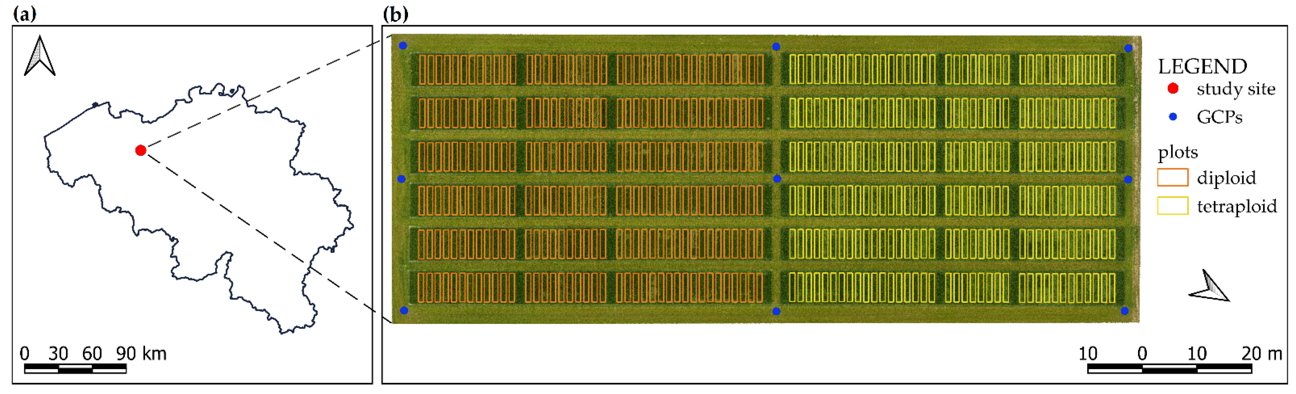
2.1. Experimental Site and Field Trial Design

The experimental site used is located in Merelbeke, Belgium (50.98 N, 3.77 E) (Figure 1a) on sandy loam soil. In 2020, the mean daily temperature and annual precipitation measured by the on-farm weather station were 12 °C and 795 mm, respectively. The monthly precipitation from April until October 2020 was 28.8, 10.9, 81.8, 38.8, 59.6, 125.9, 88.4 mm, respectively, and the mean monthly temperature reached 11.7, 13.7, 17.4, 17.4, 20.8, 16.1, 11.7 °C, respectively, with a prolonged period of warm and dry weather during spring.
A breeding trial established to test the performance of 115 diploid and 112 tetraploid varieties and breeding populations of perennial ryegrass (Lolium perenne L.) was monitored (Figure 1b). Diploid and tetraploid accessions were spatially segregated (Figure 1b). Within each group the accessions were arranged in a randomised block design with at least two replicates, rendering a total of 468 plots of 5.80 × 1.35 m (Figure 1b). Such a trial captures a broad genetic and phenotypic variation of perennial ryegrass. In addition, it generates a large disparity in fresh and dry matter yield production.
The trial was established and sown on the 7 May 2019. In the same year, it was mown multiple times and subsequently fertilised: on 27 June (65 kg ha−1 N, 30 kg ha−1 P2O5 and 115 kg ha−1 K2O), on 24 July (34 kg ha−1 N and 20 kg ha−1 K2O), on 29 August (26 kg ha−1 N, 12 kg ha−1 P2O5 and 46 kg ha−1 K2O) and 5 November (without fertilisation). In the subsequent year (2020), the trial was mown five times, following the regional standard cutting regime. It was also fertilised, on 17 March (88 kg ha−1 N and 140 kg ha−1 K), on 5 May (80 kg ha−1 N, 23 kg ha−1 P and 115 kg ha−1 K); on 2 July (74 kg ha−1 N and 80 kg ha−1 K); and on 3 August (60 kg ha−1 N, 17 kg ha−1 P and 85 kg ha−1 K).

2.2. Data Acquisition

2.2.1. UAV Data Acquisition

Before each harvest, a UAV flight was performed. The flight mission was carried out as close to the scheduled mowing date as possible, considering the optimal weather conditions (no rain, little to no wind and stable illumination conditions). We used two different sensors: (1) an RGB camera system (α6000, Sony Corporation, Tokyo, Japan) and (2) a 10-band multispectral camera (Dual Camera System, MicaSense, Seattle, USA) (Table 1). A UAV DJI Matrice 600 Pro (DJI, Shenzhen, China) platform with a mounted sensor was navigated along a pre-defined flight path. The flight altitude was set to 40 and 30 m above the ground level for the RGB and MS camera, respectively. The sensor speed for the two cameras was fixed at 6 m s−1 and 3.9 m s−1, respectively. These flight parameters and camera settings resulted in 70–70% and 80–80% side and forward overlap for the RGB and MS imagery, respectively. Images were taken in the morning and around solar noon (9 a.m.–2 p.m.). Flights with both sensors were executed on the same dates (4 May, 15 September, and 4 November 2020; Table 2). Per flight with the RGB camera, almost 200 nadir images were captured versus about 750 nadir images per spectral band for the MS sensor.
The sensors used differ in the number of bands, width along the visible/near-infrared region of the spectrum and ground sample distance. The Sony α6000 is a standard (consumer-grade) digital camera generating three channels that overlap the red, green, and blue regions of the spectrum. The MicaSense’s Dual Camera System offers double the number of bands of a standard multispectral camera by integrating the power of two sensors: the RedEdge-MX and the RedEdge-MX Blue. The reach of ten narrow bands, with additional green, red and red-edge bands, provides significantly more spectral information for advanced remote sensing of vegetation than simple RGB cameras. While the RGB camera can reach a pixel size of around 0.4 cm, the multispectral sensor provides a coarser resolution of approximately 1.8 cm. High side and forward overlap are needed to build a high-quality canopy height model (CHM) based on the Structure from Motion (SfM) principle (see Section 2.6).

2.2.2. Biomass Sampling

The trial was mown five times over the year 2020. For the purpose of this study, we considered the three cuts/growing periods (Table 2) with the higher yield production which are traditionally the cuts in spring and autumn. Above-ground biomass samples were collected with a grass plot harvester (Haldrup F-55, Haldrup, Løgstør, Denmark). The stubble height was set to 5 cm. The plot fresh matter yield (FMY) was directly measured by the plot harvester. A sub-sample of between 150 and 500 g was taken automatically by the machine. Later it was oven-dried for at least 72 h at 70 °C to determine its dry matter content (DMC). To obtain the DMY, the dried material was weighed and then extrapolated to kg ha−1.
Due to limiting weather conditions for UAV flights (strong wind, changing cloud cover, which occur frequently in Belgium), constrains from the breeders that are bound to an “ideal” harvesting moment and the size of the trial (long harvesting time), optimal execution of subsequent flight and cut was not always possible. The gap between the flight and harvest date was the largest in September (cut 4). The grass stalks were already bending across the whole field on the day of the flight, but this did not change until the harvest. Even though slight changes in vegetation growth (and produced yield) between flight and cut are possible, we asume that main growth patterns and within-field variability were captured.

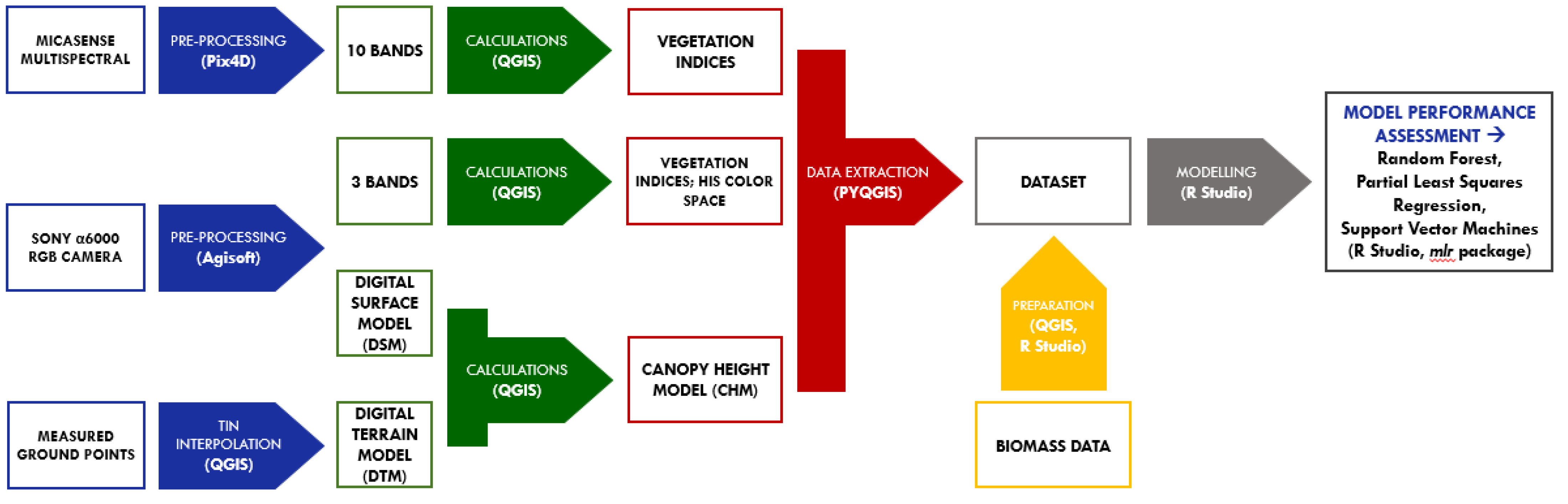
2.3. Schematic Overview of the Workflow

A schematic overview of the workflow (Figure 2) shows the steps and procedures applied for data collection, processing and modelling. The UAV-derived data were first pre-processed and stitched (blue). Generated mosaics and digital elevation models were used to calculate selected Vegetation Indices (VIs) and the Canopy Height Model (CHM) (green). To extract structural and spectral information for every plot, an integrated Python console for scripting was used to automate workflows (red). Afterwards, the obtained information was fused with biomass data (yellow). Data analysis, including principal component analysis (PCA), model calibration and validation, was performed in the last step (grey).

2.4. UAV Imagery Pre-Processing

Due to differences between the RGB and multispectral sensors, derived data were processed in the appropriate software following the procedures described in detail below.

2.4.1. RGB Camera

First, images acquired with the RGB sensor were corrected and adjusted for white balance and exposure in Lightroom v.6.5. (Adobe Systems Incorporated, San Jose, CA, USA). For this purpose, a grey reference card (18% reference grey, Novoflex Präzisionstechnik GmbH, Memmingen, Germany) was placed in the field during the flight campaign. The raw images were converted to jpeg files. Photogrammetric processing of these images was completed with Agisoft Metashape Professional v1.5.5 software (Agisoft LLC, St. Petersburg, Russia). In this study, we followed a similar processing workflow as presented in previous research [6,29]. The initial stage of photo alignment was set to a “high” quality setting, as it helps to get more accurate camera position estimates (User Manual v1.5). The key and tie point limit was set to 40,000 and 4000, respectively. Subsequently, nine Ground Control Points (GCPs), evenly spread across the field, were used for precise georeferencing to scale the model and to enhance photo alignment. The coordinates of the GCPs were determined on-site with an RTK GPS (Stonex S10 GNSS, Stonex SRL, Paderno Dugnano, Italy). Next, the optimize cameras command was selected. This executes an adjustment procedure by fine-tuning interior and exterior camera orientation parameters and correcting possible distortions. Dense point cloud generation was applied next, with “aggressive” depth filtering and “medium” quality parameter setting. To build a Digital Elevation Model (DEM), the dense cloud created in the preceding step was selected as the source data. The dense cloud data were also used to generate a polygonal mesh model with the Build Mesh command. In the last step, the mesh was chosen as a surface onto which the original images are projected and merged together to generate a georeferenced orthomosaic.

2.4.2. Multispectral Camera

To process the images obtained with the MicaSense Dual Camera System, we used Pix4D Mapper 4.5.6 software (Pix4D S.A., Prilly, Switzerland). As new 10-band imagery is not included in the Pix4D database, processing can take a long time, and reflectance maps might not be aligned. Therefore, a Rig add-on was used. A new rig model with translation values for the X and Y axis of each band was saved and used in each imagery processing session. Three main stages of image processing can be distinguished: (1) Initial Processing, (2) Point Cloud and Mesh, and (3) DSM, Orthomosaic and Index. In the first step, key points from images are automatically extracted to determine external and internal camera parameters. Similar to the Align Photos tool in Agisoft Metashape Professional, a sparse point cloud is computed. Next, to enhance the project’s global accuracy, GCPs are added and marked using rayCloud interface. The exact position of the GCP was marked on at least eight images, and automatic marking was then selected. This process was repeated for all 9 GCPs. Afterwards, the camera parameters needed to be reoptimized (external and internal locations). In the second step, a 3D point cloud and a 3D textured mesh were generated.
The last step consisted of choosing processing options for the DSM and orthomosaic generation. DSM noise filtering was applied to filter and smooth the obtained point cloud with the median altitude of neighbouring points. The surface smoothing parameter was set to “medium”. The aim of this setting is to keep features sharp while flattening nearly planar areas. The DSM was generated with the triangulation method as suggested for flat areas such as agricultural lands. The crucial setting to define is radiometric processing and calibration. The correction type was set to “Camera and Sun Irradiance” to correct the camera parameters and the sun irradiance information provided by the light sensors. The radiometric calibration target (also called the reflectance panel) was used during flight campaigns. The radiometric calibration image was taken immediately before and after each flight so that lighting and weather conditions were similar to the ones observed during the flight. The pictures of the calibration target were automatically recognised and the target region was automatically marked by the software. The reflectance factor values linked to each band were manually entered based on values provided by the target manufacturer. The reflectance panels were used for illumination adjustment, to calibrate and correct the reflectance values of images (according to the calibration target values). By applying radiometric calibration it is possible to compare data obtained with different cameras or flights.

2.5. Vegetation Indices Calculation

To calculate a set of Vegetation Indices (VIs), we used the open-source QGIS 3.12.3 with GRASS 7.8.3. software (QGIS Geographic Information System, QGIS Development Team, Open Source Geospatial Foundation). As the procedure had to be repeated multiple times over different flight dates, we used a graphical modeller interface to create a chain of VIs calculations. Models were created separately for data derived from RGB and the multispectral camera. Either a raster calculator tool or an i.vi function from the GRASS module was applied for calculations of vegetation indices.

2.5.1. RGB

Based on the RGB-derived spectral data, we selected and computed 9 VIs as candidates for biomass predictions (Table 3). Most of these VIs were developed to highlight the orthomosaic’s green component [41] and to indicate spectral variability within vegetation canopies [42]. The Excess Green Index (ExG) is one of the commonly used VIs for crop monitoring and soil masking. Combining ExG with canopy height information, especially with physical height measurements, provides good estimates of grass biomass [6]. The Excess Red index (ExR) is negatively correlated with biomass. The Excess Green minus Excess Red index (ExGR) is calculated by subtracting the ExR from the ExG index. This VI performs well when detecting green vegetation from soil and dead plant material, as it showed low sensitivity to various soil-residue backgrounds [43]. The Normalized Green-Red Difference Index (NGRDI) distinguishes vegetation from the other land cover types [44]. The Green Leaf Index (GLI) provides reliable ground cover estimates that can be used in studying persistency [45]. The Visible Atmospherically Resistant Index (VARI) was developed on the concept of the Atmospherically Resistant Vegetation Index (ARVI) to initiate an atmospheric self-correction [46]. VARI has a more linear relationship with and was more sensitive to vegetation fraction than NGRDI [46].
In addition, RGB raster map layers were transformed to an alternative colour space of hue, intensity and saturation (HIS) using the i.rgb.his tool with the GRASS module. This colour space was established to provide further representations of subjective human perceptions [47].

2.5.2. Multispectral

Criteria for selecting VIs were (i) general applicability in vegetation monitoring and (ii) quantitative assessments of growth dynamics (Table 4). The Normalized Difference Vegetation Index (NDVI), computed as a ratio in the near-infrared (NIR) and red spectral bands [52], is the most commonly used VI, including the assessment of grassland biomass [53]. Nevertheless, previous research confirms its limitations, as it saturates in dense vegetation and at high biomass [54]. By applying a weighting coefficient a, Gitelson [55] proposed the Wide Dynamic Range Vegetation Index (WDRVI) that improves the range of NDVI while still using the same spectral bands. This index is sensitive to changes at high biomass levels [56] and enhances correlation with vegetation fraction [55]. Since NDVI is also susceptible to changes in soil background and is dependent on soil brightness [57], indices like Soil Adjusted Vegetation Index (SAVI) [58], Second Modified Soil Adjusted Vegetation Index (MSAVI) [59], and Perpendicular Vegetation Index (PVI) [60] were added. They were established to reduce soil effects on canopy spectra [59] and avoid soil background noise [56]. Another essential VI that compensates for some of the NDVI shortcomings is the Enhanced Vegetation Index (EVI) [61]. EVI is computed with a combination of three reflectance bands from the NIR, red and blue regions of the spectrum. It offers a vegetation greenness measure [62], which simultaneously minimises canopy background (soil) variations and atmospheric influences such as residual contamination [61,63]. In a search for an alternative and additional index resistant to atmospheric effects, we also applied the Green Atmospherically Resistant Vegetation Index (GARI). This index is based on the ARVI concept [64], but should be more responsive to a broad range of chlorophyll (Chl-a) concentrations [65].
The Modified Chlorophyll Absorption in Reflectance Index (MCARI) proposed by Daughtry et al. [66] is a measure of chlorophyll absorption depth [67]. Previous research demonstrated its sensitivity to chlorophyll concentration changes. However, at low chlorophyll concentrations, MCARI is affected by non-photosynthetic elements [67]. To the best of our knowledge, no previous study has investigated the applicability of the Photochemical Reflectance Index (PRI) in biomass predictions of forage grasses with UAV-mounted multispectral sensors. The PRI formula is analogous to that of NDVI, but here two narrow bands from the green part of the spectrum are used. PRI indicates photosynthetic radiation efficiency [68]; however, recent studies also examined its potential for Light Use Efficiency (LUE) estimations [69]. The green Chlorophyll Index (CLg), proposed by Gitelson et al. [70] is reported to be a very good indicator of chlorophyll content. Finally, the Simple Ratio Index (SR) is a basic VI that can help distinguish green vegetation from other objects.

2.6. Canopy Height Model Calculation

Digital Surface Models (DSM), representing the top of the canopy surface, were generated using data derived from the two sensors and during three flight campaigns. The procedures and selected parameters used to create DSM are described in greater detail above (Section 2.4). In both cases, the Structure from Motion (SfM) technique was implemented to process the images. SfM has become a standard solution for a wide array of mapping applications [73], as it employs several 2-dimensional images to reconstruct the 3-dimensional structure of a selected landscape. To compute the Digital Terrain Model (DTM), we applied the Delauney Triangular Irregular Network (TIN) using TIN interpolation tool within the QGIS 3.12.3 with GRASS 7.8.3. software (QGIS Geographic Information System, QGIS Development Team, Open Source Geospatial Foundation). For this purpose, 33 ground points, evenly spread across the experimental field, were georeferenced on-site with an RTK GPS (Stonex S10 GNSS, Stonex SRL, Paderno Dugnano, Italy).
Even though all DSMs were computed using the same parameters, slight differences in the flight altitude and the overlap resulted in minor differences in pixel size. Hence, prior to Canopy Height Model (CHM) calculations, all DSM rasters were aligned to the reference DTM. We applied the Align Raster tool with the Nearest Neighbour resampling method. The canopy height (CH) was calculated by subtracting the DTM from the DSM at the pixel level. As we used two different sensors in this study, CH based on RGB camera (CHRGB) and CH based on MS sensor (CHMS) are distinguished and compared. For this purpose, the coefficient of determination (R2) using linear regression was calculated, while for error estimations root mean square error (RMSE) and relative RMSE were computed (explained in Section 2.10.1).

2.7. Data Extraction and Dataset Preparation

Polygonal shape files for each plot were created in QGIS 3.12.3 with GRASS 7.8.3. software (QGIS Geographic Information System, QGIS Development Team, Open Source Geospatial Foundation). A margin of 0.2 m and 0.3 m was excluded from the plot’s boundary to account for border effects. In the next step, we extracted median (p50) and interquartile range (IQR) statistics from VI layers and p50, p90 and IQR from CH raster layers for each plot using the v.rast.stats tool in the GRASS module. An integrated Python console for scripting was used to automate the procedure.
UAV-based canopy structural (CH) and spectral information (VIs) and their fusion were employed to predict dry matter yield (dependent variable) on a plot per plot basis. As a result, eight feature combinations were tested and compared. First, we built simple regression models (linear model, LM) with median height as the only variable separately for RGB (1.CHRGB) and MS sensor derived data (2.CHMS). These became reference models used for further comparison. Next, only spectral information was used to generate three different datasets: Vegetation Indices based on the RGB sensor data (3.VIRGB); VIs relying on RGB sensor data combined with information from HIS colour space (4.VIRGB + HIS), and VIs based on the MS sensor data (5.VIMS). In the last stage, we fused structural (canopy height) and spectral information according to the implemented sensor to build three new models: (a) 6.CHRGB + VIRGB, (b) 7.CHRGB + VIRGB + HIS, and (c) 8.CHMS + VIMS.

2.8. Principal Component Analysis

To understand relationships and uncover patterns in this complex dataset and to better understand the relations between the different VIs, a principal components analysis (PCA) was implemented. We used the FactoMineR [74] and factoextra [75] packages in R. The results were visualised using a biplot that combines score and loading plots in a single graph. A score plot projects samples (points), while a loading plot projects the variable information (vectors) over the first two PCs. Consequently, biplots highlight the most prominent patterns on how phenotypic elements vary [17]. The median value (p50) of each predictor variable per plot, both RGB and MS-based, was applied in the PCA. To make variables comparable, data were standardised before the analysis. In the analysis, ploidy level and cut were added as categorical (qualitative) supplementary variables, while measured dry matter yield was set as a continuous (quantitative) supplementary variable. These supplementary variables had no influence on the determination of the principal components.

2.9. Modelling Methods

In the modelling framework, the dry matter yield (DMY) was set as the target variable. In order to compare the sensitivity of the biomass estimation concerning ploidy level, models were built separately for diploids, tetraploids and all the plots together. We compared three machine learning algorithms: Partial Least Squares Regression (PLSR), Random Forest (RF), Support Vector Machine (SVM) with a linear model (LM). The algorithms were selected based on the differences in their mathematical approach. PLSR is a dimensionality reduction technique that performs predictor reduction to a simpler set of uncorrelated components [76]. RF is an ensemble-based classifier predicting a combination of decision trees [77]. SVM builds hyperplanes to separate classes of points with a maximal margin [78]. Mean centring and scaling of variables (data standardisation) was performed before the modelling procedure and embedded in the inner resampling loop of a nested cross-validation approach as described below.
To understand the relevance of the predictor variables used to generate an RF model and to define how such a model uses these variables to generate an accurate prediction, a variable importance measure (VIMs) was applied. Random Forest importance measures (e.g., Gini importance or permutation) have frequently been used [79] but recent research has shown that VIMs in RFs are unreliable, especially when variables differ in the number of categories or the measurement scale [79]. Bias is also present towards correlated variables with dependence structures as they are preferred in splits, thus they are assigned more importance [80,81]. To address this a new conditional permutation importance (CPI) scheme was applied with enhanced methodology from the permimp package using R v4.0.2 in RStudio v1.3.1093 (RStudio: IDE for R, R Studio Inc., Boston, MA, USA). This method improves computation stability and its interpretability [82]. To check whether the results were reliable, the procedure was repeated three times (with different seeds), and the mean variable importance measure was reported.

2.10. Model Performance Assessment

2.10.1. Nested Cross-Validation

The simplicity of cross-validation (CV) makes it a popular and widespread strategy [83] for evaluating the prediction error [84]. In k fold cross-validation, a dataset is divided into k folds, also known as partitions. A model is refitted k times, where each fold is withheld and used for model testing (validation), while all the remaining folds are utilised for model training (calibration) [83,85]. Despite all the benefits, the proper use of CV requires that all the steps like parameter tuning and model selection are incorporated in the procedure of data partitioning [84,86]. This requires a repeated nested CV technique to assess and compare model performances. Previous studies [84,85,87] have demonstrated the need for repeated CV and confirm that this approach produces robust estimates while limiting overfitting effects.
In this study, we applied the nested CV method with 10 folds in the outer resampling loop and 5 folds in the inner resampling loop with random partitioning. We repeated the process five times as a compromise between computational time requirements and randomness influence reduction. The inner resampling loop was used for hyperparameter tuning and model selection. The outer resampling loop was used for predictive performance evaluation. We implemented the procedure of nested CV in the R software, using the mlr package [88].
The performance of model predictions was quantified by computing root mean square error (RMSE) (1) and relative root mean square error (rRMSE) (2).
R M S E = 1 n i = 1 n ( y i x i ) 2
r R M S E = R M S E x ¯
where yi is the measured variable, xi is the predicted variable, n is the number of samples, and x ¯ is the average measured variable (DMY). Final performance estimates are not only across ten outer folds but also across five repetitions, totalling fifty estimate measures. Therefore, in addition to mean errors, we also report the standard deviation of errors (that relate to precision). Box plots presented in the results section are based on a summary of first quartile (Q1), median, third quartile (Q3), and upper/lower extremes with the outliers.
Pairwise comparison using Wilcoxon’s Signed Rank Test was performed to identify whether a statistically significant difference exists between the rRMSE of compared models (datasets). We selected a significance level of α = 0.05.

2.10.2. Hyperparameter Tuning

The default hyperparameter settings cannot ensure optimal model performance in a machine learning algorithm. Therefore, the hyperparameters should be optimised to achieve robust estimates [89,90]. In general, automatic optimisation should be implemented, instead of manual selection, to find the best and optimal parameter setting [90]. Hence, in this study, a grid search was applied, as it is the most commonly used approach [91].
Several hyperparameters should be set for the RF algorithm, including the number of randomly drawn variables for each split (mtry), the number of trees in a forest (num.trees), the minimum observation numbers in a node (min.node.size) or the splitting rule (splitrule) [89]. For the mtry parameter, we selected a default value that is the square root of the number of variables (rounded down). The num.trees parameter incorporated a combination of the default 500 trees, with 1000 and 1500 trees in a model. Default min.node.size parameter was set to 1 for classification, 5 for regression, and 10 for probability. We used all these values in the grid search. For the PLSR algorithm, only the ncomp parameter was tuned by using 1, 2, 4, or 6 components. It represents the maximum number of components to consider when defining the global minimum in the CV. The most critical parameters to tune in the SVM algorithm are kernel functions, degree, cost and gamma. The choice of the kernel function is the main decision [78]. Kernel function was polynomial, radial basis, or sigmoid, while degree was set to 1 (to obtain a linear approach) and 3 (as the default value for a polynomial function). The cost value controls how “soft” the margin is. Thus, low values accept more cases inside the boundary (wider margins), while higher values impose a greater penalty on including cases in the margin. Here, we optimised the cost hyperparameter using 0.1, 1, 10 and 100 values. The gamma parameter controls the influence of individual cases on the shape of the decision boundary. Here, tuning among gamma = 0.001, 0.1, 1, 3 was applied.

3. Results

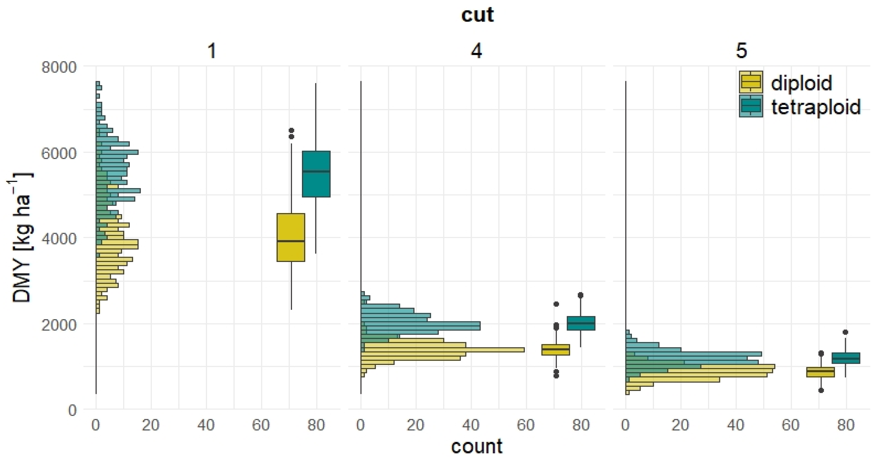
3.1. Distribution of Measured Dry Matter Yield

Measured dry matter yield (DMY) ranged between 433 kg ha−1 and 6506 kg ha−1 in diploids with a mean of 2112 kg ha−1 when all three cuts were considered. For tetraploids, DMY ranged between 733 kg ha−1 and 7595 kg ha−1 with a mean of 2905 kg ha−1 when all three cuts were taken into account (Table S1).
On average, tetraploids produced more biomass than diploids across all cuts analysed. The highest yield production was observed during the first cut, in May; 4058 kg (±854) and 5520 (±761) kg ha−1 were collected on average in the first cut for diploids and tetraploids, respectively.
Figure 3 shows that in the first cut there was the highest variability in DMY for both diploids and tetraploids. In contrast, the lowest DMY and the lowest variability was noted during the fifth cut. At this cut, on average, 882 (±160) and 1193 (±185) kg ha−1 were collected for diploids and tetraploids, respectively.

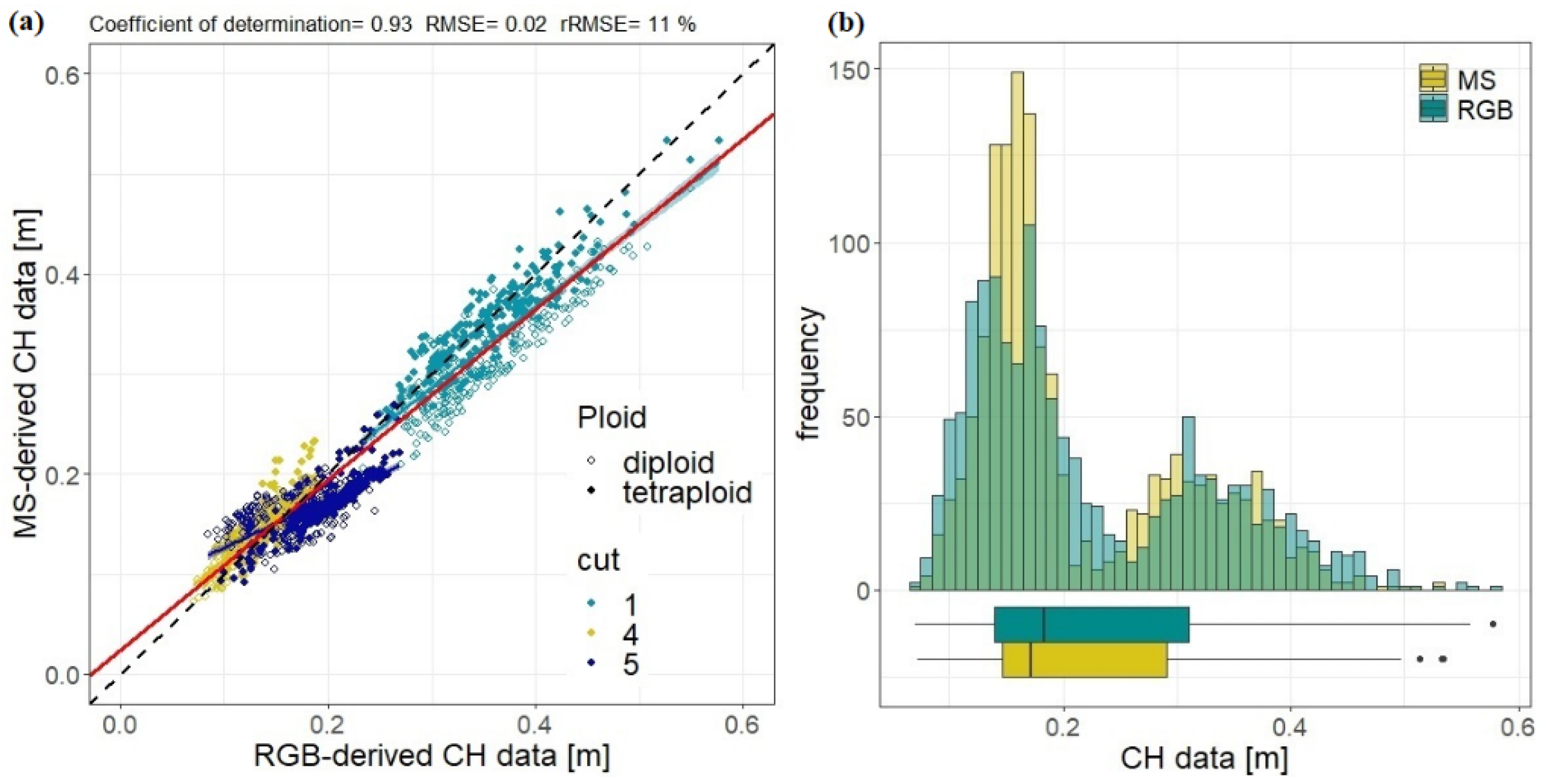
3.2. Comparison of UAV-Based Canopy Height Models Derived from Two Sensors

To generate accurate DSMs, nine GCPs were evenly distributed across the field area. The average and standard deviation error estimates (calculated as RMSE) across these GCPs for the XY-plane were 0.044 ± 0.015 and 0.035 ± 0.010 m and 0.012 ± 0.002 and 0.009 ± 0.002 m for the Z-plane for the RGB and MS imagery, respectively, showing a slightly better result for the MS sensor data.
Good agreement was found between mean CHRGB and mean CHMS (R2 = 0.93, Figure 4a), with an RMSE of 0.02 m and rRMSE of around 11%. In general, lower canopy height values (approx. −27%) were obtained with MS imagery (Figure 4b), especially for the flight taken before the fifth cut, when canopy height barely reached 0.2 m. Those CHs also yielded lower correlation values, while the highest correlation value was observed for the first cut. CH just before the first cut reached the highest values with high variability between different plots.

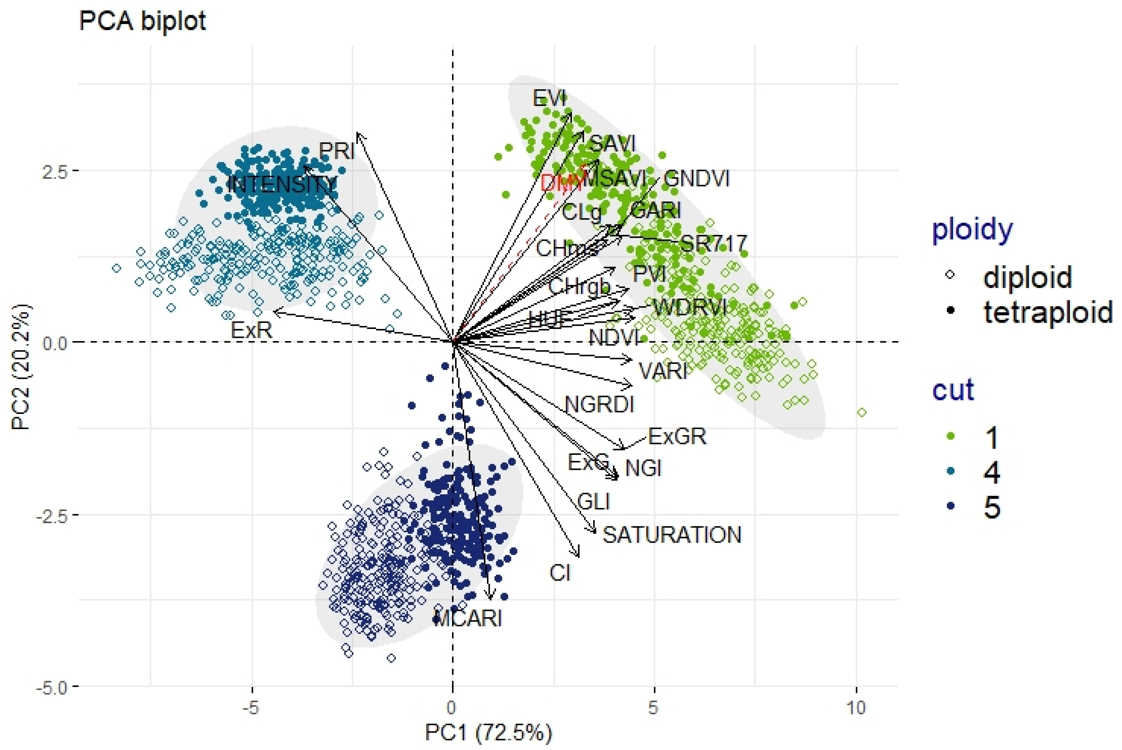
3.3. Principal Component Analysis

A PCA was carried out to evaluate the relation of all variables (CH and VIs) considered (Figure 5). A considerable fraction of the variation (92.7%) in the multi-dimensional data was explained by the first two principal components. The first axis (PC1) captured 72.5% of the present variation, while the second axis (PC2) described 20.2%. These two PCs were evaluated as a sufficient outline of the essence of the data and were retained for further data projection and visualization in a low-dimensional space.
Notable in the PCA biplot is the difference among clusters of observations associated with different cuts. Data collected at the first, fourth and fifth cut differ from each other. For data collected at the first cut, there was a considerably larger variation present for both principal components compared to the other cuts. For the fourth cut, samples showed low values for PC1 and high values for PC2, while for the fifth cut there were lower values both on the first and second PC. When considering individual cuts, one can observe similarities among plotted samples. The distances among points were greater only for the first cut, as observations spread diagonally across two dimensions (PC1 and PC2). This indicates more differences and a larger variation across observations. Differences in sample clustering were also noticeable on the ploidy level, as diploids and tetraploids grouped separately with some overlap (Figure 5). These differences between diploids and tetraploids are pronounced, for instance, in the fifth cut, as points represent different values on the PC1 axis.
A PCA biplot also projects the variable information through vectors and represents the correlation among variables. VIs grouped together with small angles, like PVI, WDRVI, HUE, NDVI or GNDVI, GARI and SR717 were all positively correlated. In contrast, PRI and CI were negatively correlated, as they were placed on opposite quadrants. The angle of 90° suggests that variables such as MSAVI and ExGR, or ExR and EVI, are not correlated and are either independent or complementary. Variables that are further away from a PC origin indicated higher quality and better representation on the factor map and thus had a bigger effect on a specific PC. Values of quality of representation (cos2) and contribution of variables (contrib) for both axes were the greatest for VIs grouped closely together, including GLI, ExGR, NGI, and ExG. Other essential variables explaining high variability in analysed PCs are WDRVI, GARI, and NDVI. NDVI and VARI variables correlated best with the PC1. This implies that high PC1 values indicate greener plants, higher vegetation vigour and coverage. Even though not closely aligned to the PC2 axis, two VIs (EVI and PRI) were positively correlated with this axis. Higher EVI values generally point out healthy vegetation and a higher leaf area index. In contrast, MCARI pointed towards lower PC2 values, which implies that in general high MCARI values signal low leaf chlorophyll content. This was in accordance with the opposite direction of the CLg vector describing the chlorophyll content. The intensity arrow points towards lower PC1 and higher PC2 values, and also in the opposite direction to the saturation arrow, indicating that the variables are negatively correlated. Observations plotted for the first cut spread out parallel to the intensity and saturation arrow, with tetraploids reaching generally higher intensity and lower saturation values than diploids. For the first cut, bending of the leaves was observed in a relatively high number of tetraploid plots. Bent leaves appeared lighter on an image (Figure 6) due to near specular light reflection, thus reaching higher intensity and lower saturation values. This was also visible in the orthomosaic of the spring cut (Figure 6).

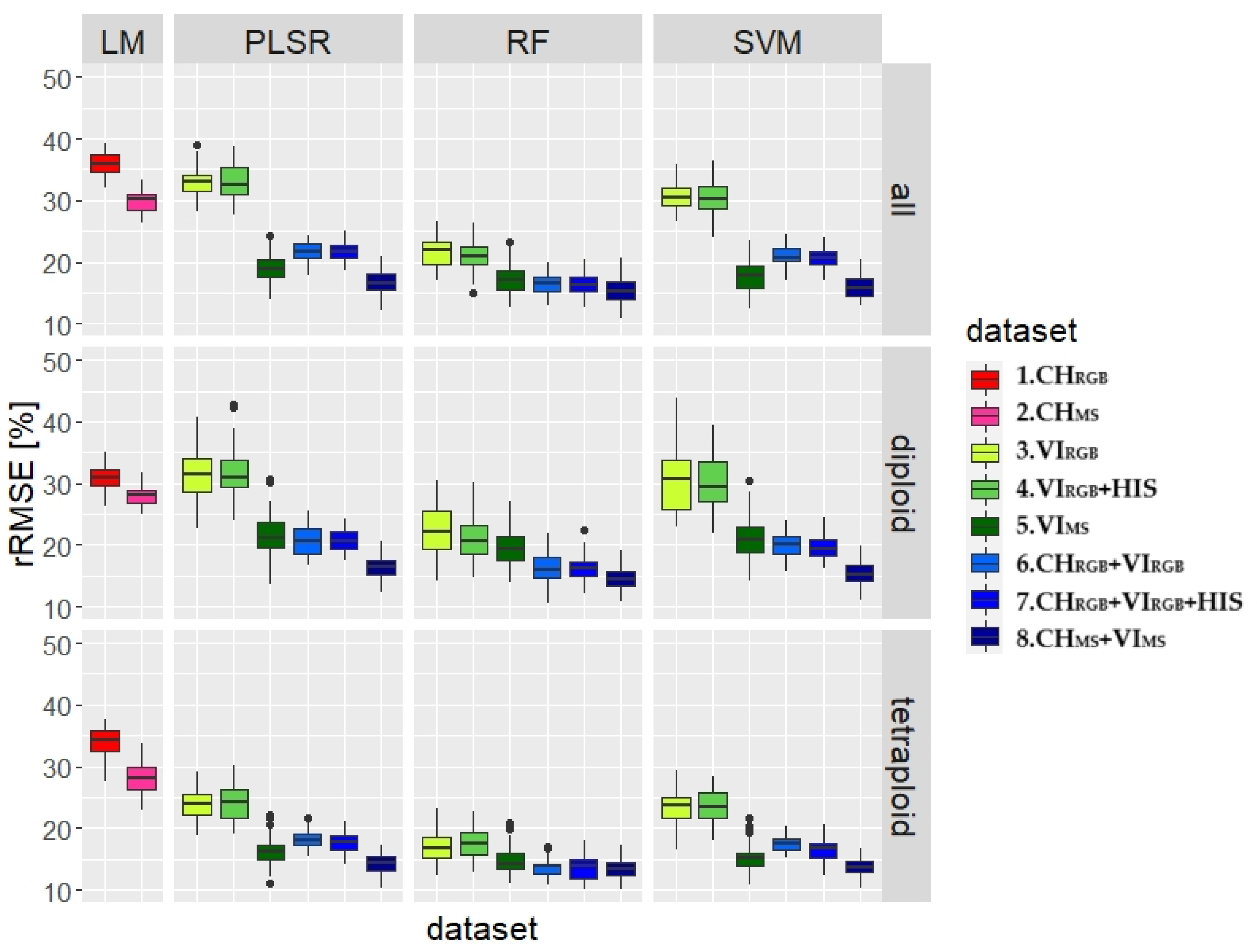
3.4. Model Building for Dry Matter Yield Predictions

DMY was modelled using canopy structural and spectral information. The framework integrated models developed for different ploidy levels (all plots, diploid, tetraploid) and three machine learning algorithms (PLSR, RF, and SVM). As predictive performances were quantified with RMSE and rRMSE estimates across 50 repetitions, the results are demonstrated as distribution box plots (Figure 7) and as mean values (Table S2).
Independent of ploidy level, CHMS proved to be a better DMY predictor variable in linear regression than CHRGB (Figure 7). The CHMS dataset also reached similar mean rRMSE values (around 30%) independent of ploidy level. This was not the case for the CHRGB dataset, where results vary among groups of observations. In general, the mean RMSE for the CHRGB dataset accounted for 897 kg ha−1 (rRMSE of 35.9%), 654 kg ha−1 (rRMSE of 31%), and 986 kg ha−1 (rRMSE of 34%) for all plots, diploids, and tetraploids, respectively.
Both PLSR and SVM share a number of similarities in their performance (Figure 7). For instance, PLSR and SVM models built with RGB-based spectral variables only (dataset 3 and 4) performed worse in yield predictions than any other feature set compared. For tetraploids only, it provided better mean error metrics than a simple linear regression built with CH information only. Visual comparison of error distribution in those feature-algorithm pairs also often indicates much more variability in predictions with a larger estimate spread. This pattern was similar for diploid, tetraploid and all varieties considered. Additionally, with both PLSR and SVM models, there was a considerable improvement in yield predictions when spectral VIs derived from the multispectral sensor were used.
Among the tested machine learning algorithms, RF performed the best on average, irrespective of the ploidy level or the dataset used. We focus on this algorithm for further comparison. In general, adding hue, intensity and saturation (HIS) features, either to RGB-based VIs or their combination with CH, produced either slightly worse, similar or slightly better average error estimates across ploidy levels. The Wilcoxon Signed Rank Test (Figure S1) for the comparisons dataset 3 vs. 4, and dataset 6 vs. 7 reached a p-value > 0.05. Thus, we failed to reject the null hypothesis that tested groups have the same predictive error and can conclude that the inclusion of HIS information did not result in substantial model improvements. Comparison of models built with spectral data derived from the RGB (3.VIRGB or 4.VIRGB + HIS) and the multispectral sensor (5.VIMS), indicates that MS-based VIs are better predictors of DMY regardless of ploidy level. In all cases, the p-value was lower than the threshold value of 0.05, meaning that the differences are statistically significant (Figure S1). For the VIMS dataset, the mean rRMSE values reached 17.2%, 19.6%, 14.9% for all plots, diploids, and tetraploids, respectively. For the VIRGB + HIS dataset, these values were higher and accounted for 21.1%, 21.1%, and 17.2%, respectively.
We also examined whether combining structural (CH) and spectral features (VIs) improved the predictions of DMY. By fusing structural and spectral information, better results were obtained for both RGB and MS sensor derived data. The results of the pairwise comparison using Wilcoxon’s Signed Rank Test demonstrated that model predictions of compared datasets (dataset 4 vs. 7, and dataset 5 vs. 8) were statistically significant (p < 0.001). Even though the improvement was more clear for the RGB-based dataset (based on the difference between mean rRMSE values), the combination of MS-based variables (8.CHms + VIms) proved to be the best DMY predictor of all (Table S2, estimates marked in red). When considering all plots in combination, the mean RMSE reached 382 kg ha−1 and rRMSE was approximately 15.3%. For diploids, the RMSE averaged 308 kg ha−1 and rRMSE 14.6%. For tetraploids, this best performing feature-algorithm pair produced the lowest rRMSE of 13.1% (mean RMSE of 380 kg ha−1). Even though MS-based predictors (CHMS + VIMS) reached the lowest mean rRMSE values, results of the Wilcoxon test for tetraploids showed that it was inconclusive whether a statistical difference exists between models built with RGB (6. CHMRGB + VIRGB) or MS-based (8.CHMS + VIMS) data (p-value = 0.27).
Another important factor to consider while comparing models is error distribution information (e.g., through box plots). Such an approach can help to understand whether (a) models are precise or not, and whether (b) the model performance is variable and dependent on the random data split. It means that it should perform well, regardless of the random data split. The interquartile range (IQR) value of error distribution (rRMSE) for the model built with the RF algorithm and CHMS + VIMS variable combination was only 2.8% (all plots), 2.4% (diploids) and 2.6% (tetraploids). In contrast, the highest IQR value of 8% was recorded for the SVM model built with RGB-based spectral data (3.VIRGB) and diploid samples, which highlights a much larger spread and variability in predictive performance. In Figure 7, it is apparent that adding MS-based CH information to MS-based VIs improved predictions (i.e., 5.VIMS vs. 8.CHMS + VIMS). However, this improvement was lower for tetraploids. It seems that datasets containing spectral features from the MS sensor only (5.VIMS) already provided very good results across all tested algorithms. Averaged rRMSE of 16.4%, 14.9% and 15.3% was reached for the PLSR, RF, and SVM algorithms, respectively.

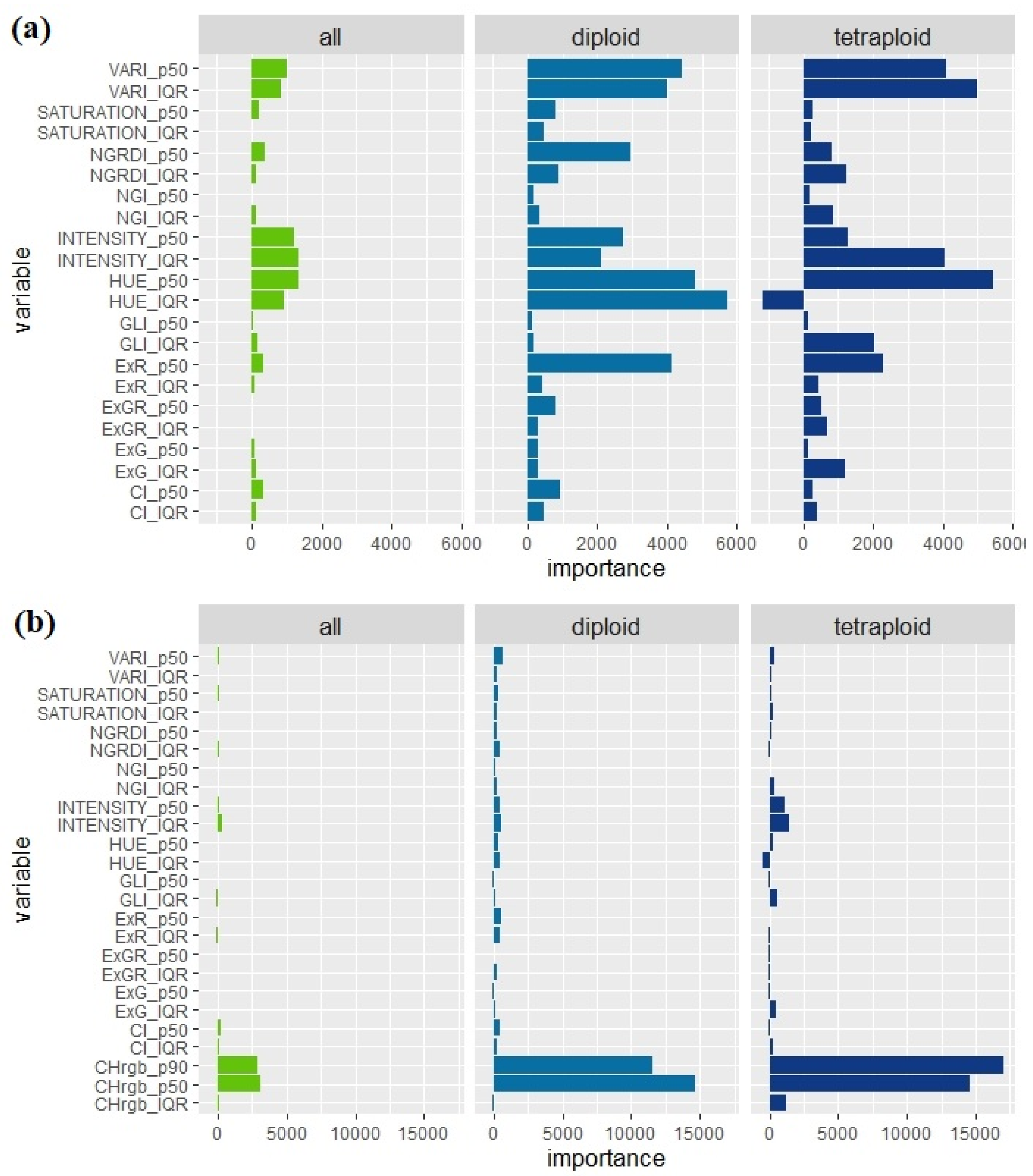
3.5. Variable Importance

To interpret which predictor variables were relevant while generating a Random Forest model, a new conditional variable importance technique was implemented [82]. The higher the importance score presented below, the more influential the predictor variable is. Figure 8 provides the results for the spectral features (a), and the changes when CH data were added (b) based on the RGB sensor. The top five important variables were similar across the analysed groups (hue, VARI, intensity, ExR, NGRDI). However, the value of the importance measure and thus the ranking varied among the groups.
For tetraploids, hue (p50), VARI (both p50 and IQR), intensity (IQR) and ExR (p50) were among the topmost important variables when building the RF model. For diploids, the most relevant features were hue (both p50 and IQR), followed by VARI (p50 and IQR), ExR (p50), NGRDI (p50), and intensity (p50 and IQR). When both ploidy levels were combined to build the RF model, intensity (both p50 and IQR), hue (p50 and IQR) and VARI (p50 and IQR) showed the most importance. While variables such as ExR and NGRDI are relevant for models built for tetraploids and diploids, they have only limited importance when all plots are taken into account.
As compared to the RGB-based variables, features derived from the multispectral sensor (Figure 9a) indicated fewer similarities between ploidy levels. When considering models built for tetraploids, EVI (IQR) and SAVI (IQR) show the most relevance in generating accurate predictions. SAVI (p50), SR717 (IQR), and EVI (p50) are the next in the ranking with lower importance values. In contrast, for diploids PVI (IQR), SR717 (p50) and GNDVI (p50) are the most relevant spectral features when predicting DMY. Comparable importance values were also obtained for SR717 (IQR), CLg (p50), EVI (p50), MSAVI (p50), and WDRVI (IQR). When all the spectral observations belonging to both diploids and tetraploids were used in the RF model, the computed importance was the highest for the SAVI (IQR) and EVI (IQR) vegetation indices. SAVI (p50), SR717 (IQR), and MSAVI (IQR) are the next in the ranking as they showed similar importance values.
By adding CH data to the spectral features (Figure 8b and Figure 9b), variable importance values change and CH features become the most dominant. This was similar across different ploidy levels and sensors used to derive the data. Even though the importance of VIs becomes very low, the pattern in their ranking remains similar.

4. Discussion

4.1. UAV-Derived Height Data: Accuracy and Characteristics

Previous work has shown that canopy height (CH) is positively correlated with grass biomass [92]. It is not surprising that a rising plate meter (RPM) is one of the tools most commonly used for physical measurements of grassland sward height [93] and the assessment of standing biomass, as it cleverly assesses both canopy height and density. However, linear relationships between RPM-based measurements and biomass are restricted in accuracy caused by canopy density, architecture and plant developmental stage [31]. Furthermore, RPM measurements do not work well in non-uniform grass swards with sparse and poor growth [6]. Borra-Serrano et al. [29] found that models built with UAV-derived canopy height information based on an RGB sensor achieved lower rRMSE values (27.6%) than models based on RPM data (31%). Hence, UAV-based canopy height estimations can replace the RPM method for biomass predictions [29]. In this study, we created CHMs separately from imagery obtained from RGB and multispectral sensors. A very good correlation was found between the CH derived from both sensors (R² = 0.93), but the MS-derived CHM delivered better predictions of DMY (rRMSE of 29.7%, all samples) than RGB-based CHM (rRMSE of 35.9%, all samples), irrespective of the ploidy level used to build the model.
This result might be explained by differences in the photogrammetric reconstruction by Structure from Motion (SfM) in the software used. Even though Agisoft Metashape and Pix4Dmapper follow a generic and similar workflow, different settings and parameters need to be selected in the image processing which are inherent to the software. Variation of the viewing geometry or defined flight altitude between tested sensors provides another possible explanation. For both sensors, sufficient overlap was set while planning the flight. However, for the RGB system a lower side and forward overlap (70%) was achieved. In addition, there were fewer RGB images where the GCPs were visible, and in some parts of the model, there was a lower number of overlapping images. This may be caused by problems with camera triggering or blurry images.

4.2. Structural and Spectral Data Fusion and Its Impact on Predictive Performance

The primary aim of this study was to investigate the potential of UAV-derived canopy height information, spectral features (VIs) and their fusion for the prediction of dry matter yield (DMY) in perennial ryegrass using two sensor types. Combining structural and spectral features delivered better performance estimates compared to models where either CH data or VIs were used alone, irrespective of the ploidy level used to build the model. By adding RGB-based height information to VIs, average rRMSE improved from 21.1% to 16.5%, from 21.1% to 16.3%, from 17.2% to 13.6% for all plots, diploids, and tetraploids, respectively. For MS-based data, similar model improvements were found: from 17.2% to 15.3% for both ploidy levels combined, from 19.6% to 14.6% for diploids, and from 14.9% to 13.1% for tetraploids.
Other studies have also tested different structural and spectral feature combinations for modelling biomass. For example, Michez et al. [94] examined the potential of imagery acquired with a UAV at a very fine spatial scale. Their experiment on mixtures of perennial ryegrass and white clover showed (as in this study) that combining sward height with spectral information (VIs and reflectance) provided the best performing model (RMSE = 900 kg ha−1). The complementarity of spectral and structural information was highlighted, even though 45% of the model variance was associated with sward height. Michez et al. [95] also utilised two sensors: an RGB and a four-band multispectral sensor. The RGB sensor was only used to obtain the height model, and the multispectral sensor was used to derive four bands and four VIs. In the present study, in which we considered a large number of plots (468 in total) and three cuts across the growing season, we confirmed the main findings of Michez et al. [95], who only collected 40 samples at one point in time. Furthermore, here, we did not only explore different predictor combinations or ploidy levels, but we also compared different learning algorithms, while Michez et al. [95] implemented simple linear regression modelling with stepwise selection to test three feature combinations.
Viljanen et al. [6] also demonstrated that prediction models of DMY based on the combination of height (referred to as 3D) and VI features achieved the best results in a timothy-meadow fescue mixture. They compared multiple linear regression (MLR) and Random Forest (RF) approaches. For the first technique, the RMSE and rRMSE (referred to as nRMSE) reached 340 kg ha−1 and 12.9%, while for the second algorithm RMSE and rRMSE were 370 kg ha−1 and 14.1%. In comparison, the lowest mean rRMSE estimates reported in our analysis for the RF regression (CH + VIs combination) was 382 kg ha−1 (15.3%), 412 kg ha−1 (16.5%) for MS-based and RGB-based variables, respectively (when all plots were considered). Thus, the models developed in both studies perform on a similar level (range), with those of Viljanen et al. [6] working slightly better. All features (CH, VIs, and bands combined) provided very good results with rRMSE of 15.1% for the RF method. In their case study, they used data collected from two sensors, including RGB and hyperspectral (red and NIR region), to compute VIs. However, the VIs were not compared but rather fused together.
A recent study by Karunaratne et al. [30] examined a series of RF models fitted with structural information (referred to as SfM in [30]), spectral information (referred to as VI in [30]), and the fusion of both (SfM + VI). They generated features from a five-band multispectral sensor in a research design very similar to that in our study. They also demonstrated that fusion of spectral and structural features outperformed the other tested models at all flying altitudes (flights at 25, 50, 75 and 100 m were compared). In general, data collected at 25 m flying altitude, which also had the highest resolution, delivered the best result, with an RMSE of 327 kg ha−1 and an rRMSE of 16.6%. For each flight altitude, the best predictive model reached an RMSE lower than 440 kg ha−1 (rRMSE values lower than 23%). In our study, the flight altitude for the multispectral sensor was set to 30 m (minimum height recommended by the sensor manual). Hence, it may be compared with the best performing model fitted with data collected at 25 m (rRMSe of 16.6%) reported by Karunaratne et al. [30]. Comparable models built in the present study with structural and spectral features reached an RMSE of 382 kg ha−1 and rRMSE of 15.3% for all samples. This implies that we achieved a slight improvement in the predictive performance, even when combining information from three cuts throughout the growing season. Another aspect similar to both compared studies is the size of the calibration dataset. In this study, a breeding trial with a wide range of varieties/populations was used to generate variation in the forage crop growth. For the experiment designed by Viljanen et al. [6], variation was achieved with different nitrogen fertilizer levels and cutting dates (96 plots in total in timothy-meadow fescue mixture). DMY reported by Viljanen et al. [6] ranged between approximately 200 kg ha−1 and 6100 kg ha−1. In a study by Karunaratne et al. [30], a number of sub-paddocks sown with perennial ryegrass were selected and weekly measurements were performed to capture spatio-temporal variability and heterogeneous nature of an analysed pasture. The pasture DMY ranged between approximately 500 kg ha−1 and 3500 kg ha−1.

4.3. Key Predictor Variables Linked to DMY Estimations

In the current study, 23 spectral variables were computed from UAV datasets comprising 11 features derived from the RGB (VIRGB and HIS), and 12 features from the MS sensor (VIs). We identified the most important predictor features within the best performing ML technique (RF) using a new conditional permutation importance (CPI) scheme [82]. VARI, intensity, hue and ExR were among the topmost important spectral variables derived from the RGB sensor (independent of the ploidy level). Features obtained from the MS sensor showed fewer similarities between ploidy levels. Overall, SAVI, EVI, SR717, PVI, and GNDVI were found to be among the most important spectral features. It is also important to note that a PCA biplot (Figure 6) showed the highest positive correlations between DMY and the following indices: MSAVI, SAVI and EVI. Results also demonstrated that CH variables become the most dominant, with the highest importance values, when fused with spectral features. These findings are similar to some extent to those reported by Viljanen et al. [6] and Karunaratne et al. [30]. The former study showed that CH features performed better than the analysed VIs when fused together in a dataset. In the latter study, it was found that at higher flying altitudes (50, 75, and 100 m), CH features were among the most important variables. For the 25 m model, no CH features were recorded among the top ten most important variables. This could be attributed to a better separation of canopy elements at higher altitudes and a better field of view useful in 3D point cloud generation [30]. Viljanen et al. [6] also noted that NIR-based VIs provided better results than the RGB-based VIs. Similarly, our models built with MS-based variables provided better results than those based on the RGB camera. Importantly, NDVI was not found across the top most important variables in the analysed modelling framework, irrespective of the ploidy level. This conclusion is therefore similar to that of Karunaratne et al. [30] and Alckmin et al. [31] who argued that predicting DMY with NDVI alone (as performed in past studies) is suboptimal. This is probably due to the saturation phenomenon when the crop reaches higher leaf area index levels. In contrast, EVI and GNDVI saturate less at higher leaf area index values and were identified as major predictor variables.

4.4. Transferability and Generality of a Model—Limitations

The essential goal of predictive modelling of forage DMY in a breeding context is to develop robust and accurate models that can capture and predict yield variability in space (over other locations/within plots) and time (over different seasons/years). Besides assessing spatial variation in the field, it should also make it possible to uncover genetic variation available in the breeding gene pool (applicability to a large set of varieties and populations). Hence, a suitable set of predictor variables must be generated that perform as explanatory model drivers [30]. In the current study, several combinations of structural and spectral features were tested with three machine learning techniques. In general, diploids and tetraploids in perennial ryegrass differ not only in anatomical aspects (e.g., larger cells and higher water content in tetraploids) but also in plant morphology. Tetraploids have larger and more intensely green leaves, but also a lower number and density of tillers than diploids [95]. These characteristics can be distinguished through remotely sensed data. Therefore, models were fitted separately for diploid and tetraploid varieties, as well as both ploidy levels combined (all plots). Models developed for diploids and tetraploids differed slightly. On average, models built with tetraploids achieved lower mean rRMSE values across all tested feature combinations and algorithms (e.g., 13.1% for the best performer) than models fitted with diploids (e.g., 14.6% for the best performer). When all varieties and populations were included in the modelling framework, the results were either slightly worse or better as compared to diploid models. Differentiating models based on the ploidy degree might be useful in the breeding programmes, as these two groups are bred separately. Nevertheless, for practical farm-scale applications, the use of more general models that encompass a wide range of varieties, and even species is necessary. Grasslands are often sown with a mixture of diploid and tetraploid cultivars or even different species. Hence, in practical terms, integrating and applying a general model, despite its slightly lower accuracy, can provide substantial benefits for farmers.
Although this study focused on different growth periods, we only considered one-year data and just three of the growth periods (three cuts). Future work should explore adding information collected in other seasons/years and locations/conditions. The methods used in this study for model performance assessment measure in- or out-of-sample accuracy, but do not allow to evaluate model generality or transferability (to other locations) [96]. Therefore, future studies will need to accommodate the factors mentioned. A modelling and validation framework with multi-year data across different field trials and independent samples should be considered and the developed models might need updating. Additional features, related to weather or soil conditions could also be tested and evaluated as model drivers in DMY predictions.

4.5. RGB vs. Multispectral Sensor for Perennial Ryegrass DMY Predictions

Due to the variation of above-ground biomass in forage grasses over space and time, it is very important to compute robust predictor variables that will perform well as model drivers. In the present study, we used a consumer-grade RGB camera and a ten-band multispectral system. As the multispectral camera provides higher spectral resolution, it could be assumed that it will also enable better DMY estimates. The results presented here demonstrate that models fitted with MS-based features provide lower mean rRMSE estimates than those based on the RGB camera. This outcome was independent of the machine learning algorithm applied. However, for the best performing algorithm (RF), the differences between data derived from two sensors were relatively smaller than for the other two algorithms. The exception to this pattern was noted for tetraploids, where models built with RGB-based features (dataset 6 and 7) and models built with MS-based features (dataset 8) statistically performed equally (p-value = 0.27). Nevertheless, it is important to note that multispectral data can be utilised in different ways, and not only for the calculation of spectral indices. Therefore, future studies should explore alternative approaches (e.g., spectral mixture analysis) and other VIs (e.g., from the red and red-edge region of the spectrum) to check the full potential of MS sensors.
Overall, there were pros and cons to using either RGB or MS-derived data. Both sensors achieved satisfactory accuracy. On one hand, consumer-grade RGB cameras are an affordable option compared with other sensors available on the market [97], and this is a considerable benefit, especially for farm-scale applications. In addition, it is possible to achieve a high spatial resolution using RGB sensors, even at relatively high flying altitudes. On the other hand, RGB cameras are limited in their spectral resolution as they provide information only from the red, green and blue parts of the spectrum. Additionally, the processing time of the RGB-based imagery takes longer than the processing of MS imagery. Common digital cameras record the reflectance as the digital numbers (DN) (ranging between 0 and 255). Even though the imagery in this study was corrected and adjusted for white balance and exposure, for multitemporal analyses of vegetation it is recommended to calibrate the DN into physical and comparable units [16]. In contrast, multispectral sensors deliver higher spectral resolution. The MS sensor used in this study captures 10 spectral bands with pixel-aligned imagery. Bands in the green, red, red edge and NIR region allow identification of unique spectral signatures. One of the main advantages of MS imagery is the presence of a downwelling light sensor, radiometric calibration target and a GPS. This makes it possible to radiometrically calibrate the images for repeatable and precise measurements without being affected by changes in environmental conditions. On the other hand, MS cameras are clearly more expensive than digital RGB cameras [98] which could be a disadvantage in practical farm-scale applications. However, distributing and sharing costs, sensors, or processing procedures among different stakeholders (e.g., local farmers, universities, government institutions) might reduce the initial investment needed and make multispectral sensors more accessible.

4.6. Comparison of Modelling Techniques

The implementation of ML algorithms in remote sensing applications (including precision agriculture) has increased recently [98]. Considering the large volumes of data collected from UAV-based sensors, ML approaches seem the proper solution as they can handle: (a) high dimensional datasets, (b) complex linear and nonlinear relationships, and (c) highly correlated features (multicollinearity issue) [30,99]. Machine learning techniques have also been used recently to generate prediction models of yield in grass swards [6,29,31].
The comparison of ML techniques carried out in this study showed that PLSR and SVM share key features in their predictive performance. When spectral variables derived from the RGB sensor (3.VIRGB) were used in the model, PLSR and SVM yielded the highest rRMSE values (33.0% and 30.7%, respectively; all samples were included in the analysis) while RF reached rRMSE of 21.5%. On average, the RF algorithm achieved the lowest error values, irrespective of the dataset used. A key study comparing similar ML regression algorithms is that of Maimaitijiang et al. [32]. In their analysis, PLSR, RF, and SVM were tested together with an extreme learning regression (ELR) to predict leaf area index, biomass and leaf nitrogen concentration in soybean. The findings demonstrated that ELR stably achieved the best performance for above-ground biomass, while SVM and RF provided comparable accuracies. At the same time, PLSR was outperformed by other models in most of the cases. Several other studies have also explored and incorporated different algorithms to estimate DMY [6,29,31,33]. Both Viljanen et al. [6] and Borra-Serrano et al. [29] reported that RF provided one of the lowest rRMSE values. Nevertheless, in both cases, RF was not the best performer, as MLR (which included all variable set combinations) provided lower error estimates. To develop above-ground biomass prediction models for legume–grass mixtures, Grüner et al., [33] used two ML algorithms: PLSR and RF. Their results showed that the best performing model (rRMSE of 10%) was built with an RF learner and a whole dataset (with texture features). A recent study by Alckmin et al. [31] also tested several regression algorithms for biomass estimations in perennial ryegrass and found that in terms of average accuracy, RF (RMSE of 405.8 hg ha−1) and STACK (RMSE of 407.6 hg ha−1) models were equivalent, with the latter rendering more precise estimations. In general, the results of the current study were similar to those reported by Alckmin et al. [31] and Grüner et al. [33]. On average, we noted a better accuracy for RF compared to other modelling techniques. In addition, an important advantage of using RF is the computation time requirements, as RF modelling was approximately three times faster than SVM modelling.

5. Conclusions

Monitoring biomass yield of perennial ryegrass is crucial in breeding and grassland management. This study investigated the potential of UAV-based structural and spectral features and their fusion to predict dry matter yield in perennial ryegrass. Models built with features derived from two sensors (RGB and multispectral) using diploid and tetraploid accessions and three machine learning techniques (PLSR, RF, SVM) were assessed and compared. Overall, combining structural (CH) and spectral (VIs) variables enhanced DMY estimations and outperformed “CH only” and “VIs only” models, regardless of the sensor or machine learning technique applied. Our modelling framework approach demonstrated that RF outperformed other algorithms (PLSR and SVM) in terms of lower mean RMSE estimates and reduced processing time. While the robustness of the methods developed needs to be validated using independent data (other accessions, other locations, other years, etc.), we demonstrated that the combination of multispectral imagery collected from a UAV with RF modelling approaches can deliver accurate predictions of DMY in perennial ryegrass.

Supplementary Materials

The following are available online at https://www.mdpi.com/article/10.3390/rs13173459/s1. Table S1: Descriptive statistics for measured dry matter yield (DMY [kg ha−1]) across different ploidy levels and three different cuts; reported DMY mean values over the cuts were used as a reference for relative root mean square error (rRMSE). Table S2: Results of Linear Model (LM), Partial Least Square Regression (PLSR), Random Forest (RF), and Support Vector Machines (SVM) methods for DMY estimation. Lowest root mean square error (RMSE) and relative RMSE per group are underlined. Figure S1: Wilcoxon Signed Rank Test results showing significance levels of adjusted p-value between compared datasets for (a) all plots, (b) diploid, and (c) tetraploid plots.

Author Contributions

Conceptualization, J.P., P.L., I.B.-S., T.D.S., J.A., A.G., G.R. and I.R.-R.; methodology, J.P., P.L., I.B.-S., T.D.S., J.A., A.G., P.Q., G.R. and I.R.-R.; formal analysis, J.P., P.L., I.B.-S.; investigation, J.P., P.L., I.B.-S., T.D.S.; data curation: J.P., J.A., A.G.; writing—original draft preparation, J.P.; writing—review and editing, P.L., I.B.-S., T.D.S., G.R., J.A., A.G., P.Q., I.R.-R. and I.A.J.; visualization, J.P., P.Q.; supervision, P.L., G.R., I.R.-R. and I.A.J. All authors have read and agreed to the published version of the manuscript.

Funding

This project has received funding from the European Union’s Horizon 2020 research and innovation programme under the Marie Skłodowska-Curie grant agreement No 813114, FutureArctic (https://www.futurearctic.be/ accessed on 20 July 2021).

Data Availability Statement

Data is publicly available at https://zenodo.org/ with DOI: 10.5281/zenodo.5337058.

Acknowledgments

The authors wish to thank Thomas Vanderstocken and Aaron Van Gehuchten for performing the UAV flights and the ILVO breeding team for trial management, harvesting and determination of DMY. Special thanks to Miriam Levenson for the English language corrections and four anonymous reviewers for their valuable feedback.

Conflicts of Interest

The authors declare no conflict of interest.

References

  1. Loveland, T.R.; Reed, B.C.; Brown, J.; O’Ohlen, D.; Zhu, Z.; Yang, L.; Merchant, J.W. Development of a global land cover characteristics database and IGBP DISCover from 1 km AVHRR data. Int. J. Remote Sens. 2000, 21, 1303–1330. [Google Scholar] [CrossRef]
  2. Blair, J.M.; Nippert, J.; Briggs, J.M. Grassland Ecology. In Ecology and the Environment. The Plant Sciences; Springer: New York, NY, USA, 2014; pp. 389–423. [Google Scholar]
  3. Hopkins, A.; Wilkins, R.J. Temperate grassland: Key developments in the last century and future perspectives. J. Agric. Sci. 2006, 144, 503–523. [Google Scholar] [CrossRef]
  4. Wilkins, P.W.; Humphreys, M.O. Progress in breeding perennial forage grasses for temperate agriculture. J. Agric. Sci. 2003, 140, 129–150. [Google Scholar] [CrossRef]
  5. Lussem, U.; Bolten, A.; Menne, J.; Gnyp, M.L.; Schellberg, J.; Bareth, G. Estimating biomass in temperate grassland with high resolution canopy surface models from UAV-based RGB images and vegetation indices. J. Appl. Remote Sens. 2019, 13, 034525. [Google Scholar] [CrossRef]
  6. Viljanen, N.; Honkavaara, E.; Näsi, R.; Hakala, T.; Niemeläinen, O.; Kaivosoja, J. A Novel Machine Learning Method for Estimating Biomass of Grass Swards Using a Photogrammetric Canopy Height Model, Images and Vegetation Indices Captured by a Drone. Agriculture 2018, 8, 70. [Google Scholar] [CrossRef] [Green Version]
  7. Huyghe, C.; de Vliegher, A.; van Gils, B.; Peeters, A. Grasslands and Herbivore Production in Europe and Effects of Common Policies. éditions Quae. 2014. [Google Scholar]
  8. Sampoux, J.-P.; Baudouin, P.; Bayle, B.; Béguier, V.; Bourdon, P.; Chosson, J.-F.; Deneufbourg, F.; Galbrun, C.; Ghesquière, M.; Noël, D.; et al. Breeding perennial grasses for forage usage: An experimental assessment of trait changes in diploid perennial ryegrass (Lolium perenne L.) cultivars released in the last four decades. Field Crop. Res. 2011, 123, 117–129. [Google Scholar] [CrossRef]
  9. Sampoux, J.P.; Baudouin, P.; Bayle, B.; Béguier, V.; Bourdon, P.; Chosson, J.F.; De Bruijn, K.; Deneufbourg, F.; Galbrun, C.; Ghesquière, M. Breeding perennial ryegrass (Lolium perenne L.) for turf usage: An assessment of genetic improvements in cultivars released in Europe, 1974–2004. Grass Forage Sci. 2013, 68, 33–48. [Google Scholar] [CrossRef]
  10. Casler, M.D.; Brummer, E.C. Theoretical expected genetic gains for among-and-within-family selection methods in perennial forage crops. Crop. Sci. 2008, 48, 890–902. [Google Scholar] [CrossRef]
  11. Resende, R.M.S.; Casler, M.D.; de Resende, M.D.V.; Maria, R.; Resende, S.; Casler, M.D. Genomic selection in forage breeding: Accuracy and methods. Crop. Sci. 2014, 54, 143–156. [Google Scholar] [CrossRef]
  12. Qiu, R.; Wei, S.; Zhang, M.; Li, H.; Sun, H.; Liu, G.; Li, M. Sensors for measuring plant phenotyping: A review. Int. J. Agric. Biol. Eng. 2018, 11, 1–17. [Google Scholar] [CrossRef] [Green Version]
  13. Campbell, Z.C.; Nirman, L.M.A. Engineering plants for tomorrow: How high-throughput phenotyping is contributing to the development of better crops. Phytochem. Rev. 2018, 17, 1329–1343. [Google Scholar] [CrossRef]
  14. Barre, P.; Asp, T.; Byrne, S.; Casler, M.; Faville, M.; Rognli, O.; Roldán-Ruiz, I.; Skøt, L.; Ghesquière, M. Chapter 19: Genomic prediction of complex traits in forage plants species. Perennial grasses case. In Genomic Prediction of Complex Traits; Series Methods in Molecular Biology; Ahmadi, N., Bartholomé, J., Eds.; Springer Nature: Basingstoke, UK, in preparation.
  15. Wang, J.; Badenhorst, P.; Phelan, A.; Pembleton, L.; Shi, F.; Cogan, N.; Spangenberg, G.; Smith, K. Using Sensors and Unmanned Aircraft Systems for High-Throughput Phenotyping of Biomass in Perennial Ryegrass Breeding Trials. Front. Plant Sci. 2019, 10, 1381. [Google Scholar] [CrossRef] [PubMed]
  16. Lussem, U.; Hollberg, J.; Menne, J.; Schellberg, J.; Bareth, G. Using calibrated RGB imagery from low-cost UAVs for grassland monitoring: Case study at the Rengen Grassland Experiment (RGE), Germany. Int. Arch. Photogramm. Remote Sens. Spat. Inf. Sci. 2017, 42, 229–233. [Google Scholar] [CrossRef] [Green Version]
  17. Han, L.; Yang, G.; Dai, H.; Yang, H.; Xu, B.; Li, H.; Long, H.; Li, Z.; Yang, X.; Zhao, C. Combining self-organizing maps and biplot analysis to preselect maize phenotypic components based on UAV high-throughput phenotyping platform. Plant Methods 2019, 15, 1–16. [Google Scholar] [CrossRef] [PubMed]
  18. Condorelli, G.E.; Maccaferri, M.; Newcomb, M.; Andrade-Sanchez, P.; White, J.W.; French, A.N.; Sciara, G.; Ward, R.; Tuberosa, R. Comparative aerial and ground based high throughput phenotyping for the genetic dissection of NDVI as a proxy for drought adaptive traits in durum wheat. Front. Plant Sci. 2018, 9, 893. [Google Scholar] [CrossRef]
  19. Haghighattalab, A.; Pérez, L.G.; Mondal, S.; Singh, D.; Schinstock, D.; Rutkoski, J.; Ortiz-Monasterio, I.; Singh, R.P.; Goodin, D.; Poland, J. Application of unmanned aerial systems for high throughput phenotyping of large wheat breeding nurseries. Plant Methods 2016, 12, 1–15. [Google Scholar] [CrossRef] [PubMed] [Green Version]
  20. Bi, J.; Mao, W.; Gong, Y. Research on image mosaic method of UAV image of earthquake emergency. In Proceedings of the 2014 The Third International Conference on Agro-Geoinformatics, Beijing, China, 11–14 August 2014; pp. 1–6. [Google Scholar] [CrossRef]
  21. Tsouros, D.C.; Bibi, S.; Sarigiannidis, P.G. A review on UAV-based applications for precision agriculture. Information 2019, 10, 349. [Google Scholar] [CrossRef] [Green Version]
  22. Aasen, H.; Honkavaara, E.; Lucieer, A.; Zarco-Tejada, P.J. Quantitative remote sensing at ultra-high resolution with UAV spectroscopy: A review of sensor technology, measurement procedures, and data correctionworkflows. Remote Sens. 2018, 10, 1091. [Google Scholar] [CrossRef] [Green Version]
  23. De Swaef, T.; Maes, W.; Aper, J.; Baert, J.; Cougnon, M.; Reheul, D.; Steppe, K.; Roldán-Ruiz, I.; Lootens, P. Applying RGB- and Thermal-Based Vegetation Indices from UAVs for High-Throughput Field Phenotyping of Drought Tolerance in Forage Grasses. Remote Sens. 2021, 13, 147. [Google Scholar] [CrossRef]
  24. Oliveira, R.A.; Näsi, R.; Niemeläinen, O.; Nyholm, L.; Alhonoja, K.; Kaivosoja, J.; Viljanen, N.; Hakala, T.; Nezami, S.; Markelin, L.; et al. Assessment of rgb and hyperspectral uav remote sensing for grass quantity and quality estimation. Int. Arch. Photogramm. Remote Sens. Spat. Inf. Sci. 2019, XLII-2/W13, 489–494. [Google Scholar] [CrossRef] [Green Version]
  25. Li, S.; Yuan, F.; Ata-Ui-Karim, S.T.; Zheng, H.; Cheng, T.; Liu, X.; Tian, Y.; Zhu, Y.; Cao, W.; Cao, Q. Combining color indices and textures of UAV-based digital imagery for rice LAI estimation. Remote Sens. 2019, 11, 1763. [Google Scholar] [CrossRef] [Green Version]
  26. Grüner, E.; Astor, T.; Wachendorf, M. Prediction of Biomass and N Fixation of Legume–Grass Mixtures Using Sensor Fusion. Front. Plant Sci. 2021, 11, 1–13. [Google Scholar] [CrossRef] [PubMed]
  27. Nocerino, E.; Dubbini, M.; Menna, F.; Remondino, F.; Gattelli, M.; Covi, D. Geometric calibration and radiometric correction of the maia multispectral camera. Int. Arch. Photogramm. Remote Sens. Spat. Inf. Sci. 2017, 42, 149–156. [Google Scholar] [CrossRef] [Green Version]
  28. Arantes, B.H.T.; Moraes, V.H.; Geraldine, A.M.; Alves, T.M.; Albert, A.M.; da Silva, G.J.; Castoldi, G. Spectral detection of nematodes in soybean at flowering growth stage using unmanned aerial vehicles. Ciênc. Rural 2021, 51, 1–9. [Google Scholar] [CrossRef]
  29. Borra-Serrano, I.; De Swaef, T.; Muylle, H.; Nuyttens, D.; Vangeyte, J.; Mertens, K.; Saeys, W.; Somers, B.; Roldán-Ruiz, I.; Lootens, P. Canopy height measurements and non-destructive biomass estimation of Lolium perenne swards using UAV imagery. Grass Forage Sci. 2019, 74, 356–369. [Google Scholar] [CrossRef]
  30. Karunaratne, S.; Thomson, A.; Morse-McNabb, E.; Wijesingha, J.; Stayches, D.; Copland, A.; Jacobs, J. The fusion of spectral and structural datasets derived from an airborne multispectral sensor for estimation of pasture dry matter yield at paddock scale with time. Remote Sens. 2020, 12, 2017. [Google Scholar] [CrossRef]
  31. de Alckmin, G.T.; Kooistra, L.; Rawnsley, R.; Lucieer, A. Comparing methods to estimate perennial ryegrass biomass: Canopy height and spectral vegetation indices. Precis. Agric. 2021, 22, 205–225. [Google Scholar] [CrossRef]
  32. Maimaitijiang, M.; Sagan, V.; Sidike, P.; Daloye, A.M.; Erkbol, H.; Fritschi, F.B. Crop monitoring using satellite/UAV data fusion and machine learning. Remote Sens. 2020, 12, 1357. [Google Scholar] [CrossRef]
  33. Grüner, E.; Wachendorf, M.; Astor, T. The potential of UAV-borne spectral and textural information for predicting aboveground biomass and N fixation in legume-grass mixtures. PLoS ONE 2020, 15, e0234703. [Google Scholar] [CrossRef]
  34. Meacham-Hensold, K.; Montes, C.; Wu, J.; Guan, K.; Fu, P.; Ainsworth, E.A.; Pederson, T.; Moore, C.; Brown, K.L.; Raines, C.; et al. High-throughput field phenotyping using hyperspectral reflectance and partial least squares regression (PLSR) reveals genetic modifications to photosynthetic capacity. Remote Sens. Environ. 2019, 231, 111176. [Google Scholar] [CrossRef]
  35. Huntington, T.; Area, B.; Berkeley, L. Machine learning to predict biomass sorghum yields under future climate scenarios. Biofuels Bioprod. Biorefin. 2020, 14, 1–12. [Google Scholar] [CrossRef]
  36. Wilkins, P.W. Breeding perennial ryegrass for agriculture. Euphytica 1991, 52, 201–214. [Google Scholar] [CrossRef]
  37. Smith, K.F.; McFarlane, N.M.; Croft, V.M.; Trigg, P.J.; Kearney, G.A. The effects of ploidy and seed mass on the emergence and early vigour of perennial ryegrass (Lolium perenne L.) cultivars. Aust. J. ExAgric. 2003, 43, 481–486. [Google Scholar] [CrossRef] [Green Version]
  38. Robins, J.G.; Lovatt, J.A. Cultivar by environment effects of perennial ryegrass cultivars selected for high water soluble carbohydrates managed under differing precipitation levels. Euphytica 2016, 208, 571–581. [Google Scholar] [CrossRef]
  39. Aper, J.; Borra-Serrano, I.; Ghesquiere, A.; De Swaef, T.; Roldán-Ruiz, I.; Lootens, P.; Baert, J. Yield estimation of perennial ryegrass plots in breeding trials using UAV images. Res. Collect. 2019, 312–314. [Google Scholar]
  40. Gebremedhin, A.; Badenhorst, P.; Wang, J.; Shi, F.; Breen, E.; Giri, K.; Spangenberg, G.C.; Smith, K. Development and Validation of a Phenotyping Computational Workflow to Predict the Biomass Yield of a Large Perennial Ryegrass Breeding Field Trial. Front. Plant Sci. 2020, 11, 689. [Google Scholar] [CrossRef] [PubMed]
  41. Torres-Sánchez, J.; Peña, J.M.; de Castro, A.I.; López-Granados, F. Multi-temporal mapping of the vegetation fraction in early-season wheat fields using images from UAV. Comput. Electron. Agric. 2014, 103, 104–113. [Google Scholar] [CrossRef]
  42. Li, W.; Niu, Z.; Chen, H.; Li, D.; Wu, M.; Zhao, W. Remote estimation of canopy height and aboveground biomass of maize using high-resolution stereo images from a low-cost unmanned aerial vehicle system. Ecol. Indic. 2016, 67, 637–648. [Google Scholar] [CrossRef]
  43. Meyer, G.E.; Neto, J.C. Verification of color vegetation indices for automated crop imaging applications. Comput. Electron. Agric. 2008, 63, 282–293. [Google Scholar] [CrossRef]
  44. Tucker, C.J. Red and photographic infrared linear combinations for monitoring vegetation. Remote Sens. Environ. 1979, 8, 127–150. [Google Scholar] [CrossRef] [Green Version]
  45. Borra-Serrano, I.; De Swaef, T.; Aper, J.; Ghesquiere, A.; Mertens, K.; Nuyttens, D.; Saeys, W.; Somers, B.; Vangeyte, J.; Roldán-Ruiz, I.; et al. Towards an objective evaluation of persistency of Lolium perenne swards using UAV imagery. Euphytica 2018, 214, 1–18. [Google Scholar] [CrossRef]
  46. Gitelson, A.A.; Kaufman, Y.J.; Stark, R.; Rundquist, D. Novel algorithms for remote estimation of vegetation fraction. Remote Sens. Environ. 2002, 80, 76–87. [Google Scholar] [CrossRef] [Green Version]
  47. Hernández-Hernández, J.L.; García-Mateos, G.; González-Esquiva, J.M.; Escarabajal-Henarejos, D.; Ruiz-Canales, A.; Molina-Martínez, J.M. Optimal color space selection method for plant/soil segmentation in agriculture. Comput. Electron. Agric. 2016, 122, 124–132. [Google Scholar] [CrossRef]
  48. Woebbecke, D.M.; Meyer, G.E.; von Bargen, K.; Mortensen, D.A. Color indices for weed identification under various soil, residue, and lighting conditions. Trans. Am. Soc. Agric. Eng. 1995, 38, 259–269. [Google Scholar] [CrossRef]
  49. Meyer, G.E.; Hindman, T.; Laksmi, K. Machine vision detection parameters for plant species identification. Precis. Agric. Biol. Qual. 1999, 3543, 327–335. [Google Scholar]
  50. Camargo Neto, J. A Combined Statistical-Soft Computing Approach for Classification and Mapping Weed Species in Minimum-Tillage Systems; The University of Nebraska-Lincoln: Lincoln, NE, USA, 2004. [Google Scholar]
  51. Gobron, N.; Pinty, B.; Verstraete, M.M.; Widlowski, J. Advanced Vegetation Indices Optimized for Up-Coming Sensors: Design, Performancem and Applications. IEEE Trans. Geosci. Remote Sens. 2000, 38, 2489–2505. [Google Scholar]
  52. Rouse, J.W.; Haas, R.H.; Schell, J.A.; Deering, D.W. Monitoring vegetation systems in the Great Plains with ERTS. NASA Spec. Publ. 1974, 351, 309. [Google Scholar]
  53. Mutanga, O.; Skidmore, A.K. Narrow band vegetation indices overcome the saturation problem in biomass estimation. Int. J. Remote Sens. 2004, 25, 3999–4014. [Google Scholar] [CrossRef]
  54. Thenkabail, P.S.; Smith, R.B.; de Pauw, E. Hyperspectral vegetation indices and their relationships with agricultural crop characteristics. Remote Sens. Environ. 2000, 71, 158–182. [Google Scholar] [CrossRef]
  55. Gitelson, A.A. Wide Dynamic Range Vegetation Index for Remote Quantification of Biophysical Characteristics of Vegetation. J. Plant. Physiol. 2004, 161, 165–173. [Google Scholar] [CrossRef] [PubMed] [Green Version]
  56. Towers, P.C.; Strever, A.; Poblete-Echeverría, C. Comparison of vegetation indices for leaf area index estimation in vertical shoot positioned vine canopies with and without grenbiule hail-protection netting. Remote Sens. 2019, 11, 1073. [Google Scholar] [CrossRef] [Green Version]
  57. Huete, A.R.; Jackson, R.D.; Post, D.F. Spectral response of a plant canopy with different soil backgrounds. Remote Sens. Environ. 1985, 17, 37–53. [Google Scholar] [CrossRef]
  58. Huete, A.R. A soil-adjusted vegetation index (SAVI). Remote Sens. Environ. 1988, 25, 295–309. [Google Scholar] [CrossRef]
  59. Qi, J.; Chehbouni, A.; Huete, A.R.; Kerr, Y.H.; Sorooshian, S. A modified soil adjusted vegetation index. Remote Sens. Environ. 1994, 48, 119–126. [Google Scholar] [CrossRef]
  60. Richardson, A.J.; Wiegand, C.L. Distinguishing vegetation from soil background information. Photogramm. Eng. Remote Sens. 1977, 43, 1541–1552. [Google Scholar]
  61. Huete, A.R.; Liu, H.Q.; Batchily, K.; van Leeuwen, W. A comparison of vegetation indices over a global set of TM images for EOS-MODIS. Remote Sens. Environ. 1997, 59, 440–451. [Google Scholar] [CrossRef]
  62. Gurung, R.B.; Breidt, F.J.; Dutin, A.; Ogle, S.M. Predicting Enhanced Vegetation Index (EVI) curves for ecosystem modeling applications. Remote Sens. Environ. 2009, 113, 2186–2193. [Google Scholar] [CrossRef]
  63. Jiang, Z.; Huete, A.R.; Didan, K.; Miura, T. Development of a two-band enhanced vegetation index without a blue band. Remote Sens. Environ. 2008, 112, 3833–3845. [Google Scholar] [CrossRef]
  64. Kaufman, Y.J.; Tanre, D. Atmospherically resistant vegetation index (ARVI) for EOS-MODIS. IEEE Trans. Geosci. Remote Sens. 1992, 30, 260–271. [Google Scholar] [CrossRef]
  65. Gitelson, A.A.; Kaufman, Y.J.; Merzlyak, M.N. Use of a green channel in remote sensing of global vegetation from EOS-MODIS. Remote Sens. Environ. 1996, 58, 289–298. [Google Scholar] [CrossRef]
  66. Daughtry, C.S.T.; Walthall, C.L.; Kim, M.S.; de Colstoun, E.B.; McMurtrey, J.E. Estimating Corn Leaf Chlorophyll Concentration from Leaf and Canopy Reflectanc. Remote Sens. Environ. 2000, 74, 229–239. [Google Scholar] [CrossRef]
  67. Haboudane, D.; Miller, J.R.; Tremblay, N.; Zarco-Tejada, P.J.; Dextraze, L. Integrated narrow-band vegetation indices for prediction of crop chlorophyll content for application to precision agriculture. Remote Sens. Environ. 2002, 81, 416–426. [Google Scholar] [CrossRef]
  68. Peñuelas, J.; Filella, J.; Gamon, J.A. Assessment of photosynthetic radiation-use efficiency with spectral reflectance. New Phytol. 1995, 131, 291–296. [Google Scholar] [CrossRef]
  69. Kováč, D.; Veselovská, P.; Klem, K.; Večeřová, K.; Ač, A.; Peñuelas, J.; Urban, O. Potential of photochemical reflectance index for indicating photochemistry and light use efficiency in leaves of European beech and Norway spruce trees. Remote Sens. 2018, 10, 1202. [Google Scholar] [CrossRef] [Green Version]
  70. Gitelson, A.A.; Gritz, Y.; Merzlyak, M.N. Relationships between leaf chlorophyll content and spectral reflectance and algorithms for non-destructive chlorophyll assessment in higher plant leaves. J. Plant. Physiol. 2003, 160, 271–282. [Google Scholar] [CrossRef] [PubMed]
  71. Gamon, J.A.; Penuelas, J.; Gield, B. A narrow-waveband spectral index that tracks diurnal changes in photosynthetic efficiency. Remote Sens. Environ. 1992, 41, 35–44. [Google Scholar] [CrossRef]
  72. Birth, G.S.; McVey, G.R. Measuring the Color of Growing Turf with a Reflectance Spectrophotometer. Agron. J. 1968, 60, 640–643. [Google Scholar] [CrossRef]
  73. Nesbit, P.R.; Hugenholtz, C.H. Enhancing UAV-SfM 3D model accuracy in high-relief landscapes by incorporating oblique images. Remote Sens. 2019, 11, 239. [Google Scholar] [CrossRef] [Green Version]
  74. Le, S.; Josse, J.; Husson, F. FactoMineR: An R Package for Multivariate Analysis. J. Stat. Softw. 2008, 25, 1–18. [Google Scholar] [CrossRef] [Green Version]
  75. Kassambara, A.; Mundt, F. Factoextra: Extract and Visualize the Results of Multivariate Data Analyses. R Package Version 1.0.7. 2020. Available online: https://CRAN.R-project.org/package=factoextra (accessed on 20 July 2021).
  76. Geladi, P.; Kowalski, B.R. Partial Least Squares Regression: A tutorial. Anal. Chim. Acta 1986, 185, 1–17. [Google Scholar] [CrossRef]
  77. Breiman, L. Random forests. Mach. Learn. 2001, 45, 5–32. [Google Scholar] [CrossRef] [Green Version]
  78. Cristianini, N.; Schölkopf, B. Support vector machines and kernel methods: The new generation of learning machines. AI Mag. 2002, 23, 31–42. [Google Scholar]
  79. Strobl, C.; Boulesteix, A.L.; Zeileis, A.; Hothorn, T. Bias in random forest variable importance measures: Illustrations, sources and a solution. BMC Bioinform. 2007, 8, 25. [Google Scholar] [CrossRef] [Green Version]
  80. Nicodemus, K.K.; Malley, J.D.; Strobl, C.; Ziegler, A. The behaviour of random forest permutation-based variable importance measures under predictor correlation. BMC Bioinform. 2010, 11, 1–13. [Google Scholar] [CrossRef] [Green Version]
  81. Strobl, C.; Boulesteix, A.-L.L.; Kneib, T.; Augustin, T.; Zeileis, A. Conditional variable importance for random forests. BMC Bioinform. 2008, 9, 1–11. [Google Scholar] [CrossRef] [PubMed] [Green Version]
  82. Debeer, D.; Strobl, C. Conditional permutation importance revisited. BMC Bioinform. 2020, 21, 1–30. [Google Scholar] [CrossRef] [PubMed]
  83. Arlot, S.; Celisse, A. A survey of cross-validation procedures for model selection. Stat. Surv. 2010, 4, 40–79. [Google Scholar] [CrossRef]
  84. Varma, S.; Simon, R. Bias in error estimation when using cross-validation for model selection. BMC Bioinform. 2006, 7, 1–8. [Google Scholar] [CrossRef] [PubMed] [Green Version]
  85. Krstajic, D.; Buturovic, L.J.; Leahy, D.E.; Thomas, S. Cross-validation pitfalls when selecting and assessing regression and classification models. J. Cheminform. 2014, 6, 1–15. [Google Scholar] [CrossRef] [PubMed] [Green Version]
  86. Schiffner, J.; Bischl, B.; Lang, M.; Richter, J.; Jones, Z.M.; Probst, P.; Pfisterer, F.; Gallo, M.; Kirchhoff, D.; Kühn, T.; et al. mlr Tutorial. arXiv 2016, arXiv:1609.06146. [Google Scholar]
  87. Vabalas, A.; Gowen, E.; Poliakoff, E.; Casson, A.J. Machine learning algorithm validation with a limited sample size. PLoS ONE 2019, 14, 1–20. [Google Scholar] [CrossRef]
  88. Bischl, B.; Lang, M.; Kotthoff, L.; Schiffner, J.; Richter, J.; Studerus, E.; Casalicchio, G.; Jones, Z. mlr: Machine Learning in R. J. Mach. Learn. Res. 2016, 17, 1–5. [Google Scholar]
  89. Probst, P.; Wright, M.; Boulesteix, A. Hyperparameters and Tuning Strategies for Random Forest. Wiley Interdiscip. Rev. Data Min. Knowl. 2019, 9, 1–19. [Google Scholar] [CrossRef] [Green Version]
  90. Schratz, P.; Muenchow, J.; Iturritxa, E.; Richter, J.; Brenning, A. Hyperparameter tuning and performance assessment of statistical and machine-learning algorithms using spatial data. Ecol. Modell. 2019, 406, 109–120. [Google Scholar] [CrossRef] [Green Version]
  91. Bergstra, J.; Bengio, Y. Random Search for Hyper-Parameter Optimization. J. Mach. Learn. Res. 2012, 13, 281–305. [Google Scholar]
  92. Virkajärvi, P. Comparison of Three Indirect Methods for Prediction of Herbage Mass on Timothy-Meadow Fescue Pastures. Acta Agric. Scand. Sect. B Soil Plant. Sci. 1999, 49, 75–81. [Google Scholar] [CrossRef]
  93. Nakagami, K. Effects of sites and years on the coefficients of rising plate meter calibration under varying coefficient models. Grassl. Sci. 2016, 62, 128–132. [Google Scholar] [CrossRef]
  94. Michez, A.; Lejeune, P.; Bauwens, S.; Herinaina, A.A.L.; Blaise, Y.; Muñoz, E.C.; Lebeau, F.; Bindelle, J. Mapping and monitoring of biomass and grazing in pasture with an unmanned aerial system. Remote Sens. 2019, 11, 473. [Google Scholar] [CrossRef] [Green Version]
  95. Balocchi, O.A.; López, I.F. Herbage production, nutritive value and grazing preference of diploid and tetraploid perennial ryegrass cultivars (Lolium perenne L.). Chil. J. Agric. Res. 2009, 69, 331–339. [Google Scholar] [CrossRef] [Green Version]
  96. Wenger, S.J.; Olden, J.D. Assessing transferability of ecological models: An underappreciated aspect of statistical validation. Methods Ecol. Evol. 2012, 3, 260–267. [Google Scholar] [CrossRef]
  97. Barbedo, J.G.A. A review on the use of unmanned aerial vehicles and imaging sensors for monitoring and assessing plant stresses. Drones 2019, 3, 40. [Google Scholar] [CrossRef] [Green Version]
  98. Castro, W.; Junior, J.M.; Polidoro, C.; Osco, L.P.; Gonçalves, W.; Rodrigues, L.; Santos, M.; Jank, L.; Barrios, S.; Valle, C.; et al. Deep learning applied to phenotyping of biomass in forages with UAV-based RGB imagery. Sensors 2020, 17, 4802. [Google Scholar] [CrossRef] [PubMed]
  99. Belgiu, M.; Drăgu, L. Random forest in remote sensing: A review of applications and future directions. ISPRS J. Photogramm. Remote Sens. 2016, 114, 24–31. [Google Scholar] [CrossRef]
Figure 1. Schematic overview of (a) the study site location in Merelbeke, Belgium, and (b) the experimental plot design with diploid and tetraploid varieties and breeding populations.
Remotesensing 13 03459 g001
Figure 2. A schematic workflow illustrating the procedures of data collection, processing and modelling.
Remotesensing 13 03459 g002
Figure 3. Histogram plots and box plots for the dry matter yield [kg ha−1] estimates across three cuts.
Remotesensing 13 03459 g003
Figure 4. Comparison of the UAV-derived Canopy Height Model (CHM) based on two sensors; (a) linear regression of mean CHM between two paired datasets derived from the multispectral (MS) vs. RGB camera systems. A regression line was fitted separately for each cut and for the whole dataset (red solid line); (b) distribution of mean canopy height information derived from multispectral and RGB camera visualized on histograms and box plots.
Remotesensing 13 03459 g004
Figure 5. A biplot of the first two dimensions (PC1 and PC2) of a principal component analysis carried out on the plot scores for the CH and VIs values based on RGB and MS imagery. Dots indicate median values per plot and are labelled according to cut and ploidy level. Vectors are loadings that project the variable information over the first two PCs. The dry matter yield (DMY, indicated as a red dashed line) data are presented as a quantitative supplementary variable, but was not included in the analysis.
Remotesensing 13 03459 g005
Figure 6. Close-up view of bending plots for some tetraploid varieties just before the first spring cut.
Remotesensing 13 03459 g006
Figure 7. Box plots of relative root mean square error (rRMSE, %) computed for each tested dataset and learning algorithms (linear model (LM), Partial Least Squares Regression (PLSR), Random Forest (RF), Support Vector Machine (SVM)). RGB-based (1.CHRGB) and MS-based canopy height model information (2.CHMS) was used as a reference model. Vegetation Indices based on RGB sensor (3.VIRGB); Vegetation Indices relying on RGB camera combined with information from HIS colour space (4.VIRGB + HIS), and finally, Vegetation Indices based on MS sensor (5.VIMS) were selected as spectral features. In the last step, structural and spectral information were fused together (6.CHRGB + VIRGB), (7.CHRGB + VIRGB + HIS), and (8.CHMS + VIMS). Models were built with data collected separately before all three cuts for diploid, tetraploid and both ploidy levels combined (all plots).
Remotesensing 13 03459 g007
Figure 8. Random forest variable importance plot showing predictor variables based on RGB sensor: (a) VIs, (b) VIs combined with CH information relevant in predicting dry matter yield of perennial ryegrass for all, diploid, and tetraploid tested plots.
Remotesensing 13 03459 g008
Figure 9. Random forest variable importance plot showing predictor variables based on MS sensor: (a) VIs (b) VIs combined with CH information relevant in predicting dry matter yield of perennial ryegrass for all, diploid, and tetraploid tested plots.
Remotesensing 13 03459 g009
Table 1. Unmanned aerial vehicle (UAV) data acquisition details.
Sensor TypeSensor BrandSensor Bands (nm)Ground Sample Distance (GSD)Flight AltitudeSide-Forward Overlap
RGBSony α6000
35 mm
red, green, and blue~0.4 cm40 m70–70%
MultispectralRedEdge-MX and RedEdge-MX blue(Dual Camera Kit)coastal blue (444), blue (475), green (531), green (560), red (650), red (668), red edge (705), red edge (717), red edge (740), NIR (842)~1.8 cm30 m80–80%
Table 2. Biomass sampling information (* information on one sample missing).
Cut/Growth Period (GP)Harvest DateNumber of SamplesUAV Flight Date
1 November 2019–May 20204/5 May 2020467 *4 May 2020
4 July 2020–September 202021/22 September 202046815 September 2020
5 September 2020–November 20205/6 November 20204684 November 2020
Table 3. List of Vegetation Indices (VIs) derived from the RGB camera system.
Vegetation IndexFormulaReference
(Normalized) Excess Green E x G = ( 2 G R B ) ( R + G + B ) [48]
(Normalized) Excess Red E x R = ( 1.4 R G ) ( R + G + B ) [49]
Excess Green—Excess RedExGR = ExG − ExR[50]
Normalized Green-Red Difference Index N G R D I = ( G R ) ( G + R ) [44]
Green Leaf Index G L I = ( 2 G R B ) ( 2 G + R + B ) [51]
Visible Atmospherically Resistant Index V A R I = ( G R ) ( G + R B ) [46]
Normalized Green Intensity N G I = G ( R + G + B ) [48]
Colouration Index C I = ( R B ) R https://www.indexdatabase.de/search/?s=color (acessed on 1 December 2020)
Table 4. List of Vegetation Indices (VIs) derived from the multispectral sensor. Abbreviations besides each band correspond to centre wavelengths in nm.
Vegetation IndexFormulaUseReference
Normalized Difference Vegetation Index N D V I = NIR 842 red 668 NIR 842 + red 668 to detect plants greenness, green biomass and phenology[52]
Green Normalized Difference Vegetation Index G N D V I = NIR 842 green 531 NIR 842 + green 531 to detect green biomass, nitrogen concentration, LAI estimation,[65]
Wide Dynamic Range Vegetation Index W D R V I = α NIR 842 red 668 α NIR 842 + red 668 sensitive at high LAI[55]
Soil Adjusted Vegetation Index S A V I = ( 1 + 0.5 ) ( NIR 842 red 650 ) ( NIR 842 + red 650 + 0.5 ) to correct for the soil brightness influence when vegetative cover is low[58]
Second Modified Soil Adjusted Vegetation IndexMSAVI = (1/2) ∗ (2 ∗ NIR842 + 1 − sqrt((2 ∗ NIR842 +1)2 − 8 ∗ (NIR842 − red668)))to minimize the effect of soil[59]
Perpendicular Vegetation IndexPVI = sin(a)NIR842 − cos(a)red668to correct for the soil influence[60]
Enhanced Vegetation Index E V I = 2.5 ( NIR 842 red 650 )   ( 1 + NIR + 6 red 650 7.5 blue 444 ) to detect green biomass, canopy greenness and phenology[61]
Green Atmospherically Resistant Vegetation Index G A R I = NIR 842 ( green 531 ( blue 444 red 650 ) NIR 842 + ( green 531 ( blue 444 red 650 ) to sense the chlorophyll concentration, the photosynthesis rate and to monitor plant stress[65]
Modified Chlorophyll Absorption in Reflectance IndexMCARI = ((rededge705 − red668) − 0.2 ∗ (rededge705 − green560)) ∗ (rededge705/red668)to measure chlorophyll concentration, canopy phenology and senescence[66]
Photochemical Reflectance Index P R I = green 531   green 560 green 531 +   green 560 to measure of the light-use efficiency, water stress detection[71]
Chlorophyll Index GreenCLg = NIR842/green531 − 1to estimate chlorophyll content[70]
Simple RatioSR = NIR/rededge717to detect green vegetation[72]
Publisher’s Note: MDPI stays neutral with regard to jurisdictional claims in published maps and institutional affiliations.

