MSNet: A Multi-Stream Fusion Network for Remote Sensing Spatiotemporal Fusion Based on Transformer and Convolution

Abstract

Remote sensing products with high temporal and spatial resolution can be hardly obtained under the constrains of existing technology and cost. Therefore, the spatiotemporal fusion of remote sensing images has attracted considerable attention. Spatiotemporal fusion algorithms based on deep learning have gradually developed, but they also face some problems. For example, the amount of data affects the model’s ability to learn, and the robustness of the model is not high. The features extracted through the convolution operation alone are insufficient, and the complex fusion method also introduces noise. To solve these problems, we propose a multi-stream fusion network for remote sensing spatiotemporal fusion based on Transformer and convolution, called MSNet. We introduce the structure of the Transformer, which aims to learn the global temporal correlation of the image. At the same time, we also use a convolutional neural network to establish the relationship between input and output and to extract features. Finally, we adopt the fusion method of average weighting to avoid using complicated methods to introduce noise. To test the robustness of MSNet, we conducted experiments on three datasets and compared them with four representative spatiotemporal fusion algorithms to prove the superiority of MSNet (Spectral Angle Mapper (SAM) < 0.193 on the CIA dataset, erreur relative global adimensionnelle de synthese (ERGAS) < 1.687 on the LGC dataset, and root mean square error (RMSE) < 0.001 on the AHB dataset).

1. Introduction

At present, remote sensing images are mainly derived from many types of sensors. One type is the Moderate Resolution Imaging Spectrometer (MODIS), and the rest are Landsat series, Sentinel and some other types of data. The Landsat series is equipped with three sensors, including Enhanced Thematic Mapper Plus (“ETM+”), Thematic Mapper (“TM”), Operational Land Imager (“OLI”) and Thermal Infrared Sensor (“TIRS”). MODIS sensors are mainly mounted on Terra and Aqua satellites, which can circle the earth in half a day or a day, and the data they obtain have a high temporal resolution. MODIS data (coarse images) have sufficient time information, but their spatial resolution is very low, reaching only 250–1000 m [1]. On the contrary, the data (fine images) acquired by Landsat have a higher spatial resolution, which can reach 15 m or 30 m, and the data can capture sufficient surface detail information, but their temporal resolution is very low, and it takes 16 days for Landsat to circle the earth [1]. In practical research applications, we often need remote sensing images with both high temporal and high spatial resolution. For example, images with high spatiotemporal resolution can be used to study surface changes in heterogeneous regions [2,3], vegetation seasonal monitoring [4], real-time mapping of natural disasters such as floods [5], land cover changes [6] and so on. However, due to current technical constraints and cost constraints, and the existence of noise such as cloud cover in some areas, it is difficult to directly obtain remote sensing products with a high spatial and temporal resolution that can be used for research, and a single high-resolution image does not meet the actual demand. To solve such problems, spatiotemporal fusion has attracted much attention in recent decades. It is used to fuse two types of images through a specific method, to obtain images with a high spatial and temporal resolution that are practical for research [7,8].

2. Related Works

Generally speaking, the existing spatiotemporal fusion methods can be subdivided into four categories: reconstruction-based, unmixing-based, dictionary-based learning, and deep learning-based methods.

The essence of the reconstruction-based algorithm is to calculate the weights of similar adjacent pixels in the input spectral information and to add them. The spatiotemporal adaptive fusion algorithm (STARFM) is the first method to use reconstruction for fusion [8]. In STARFM, the change in reflection of the pixels between the coarse image and the fine image should be continuous, and the weight of adjacent pixels can be calculated to reconstruct the surface reflection image with high spatial resolution. Because it requires a large amount of calculation and the reconstruction effect of heterogeneous regions needs to be improved, Zhu et al., made improvements and proposed an enhanced version of STARFM (ESTARFM) [9]. They used two different coefficients to process the weights of neighbouring pixels in homogeneous and heterogeneous regions to achieve a better result. Inspired by STARFM, a new data fusion model for high spatial- and temporal-resolution mapping of forest disturbance based on Landsat and MODIS (STAARCH) [10] was used to map reflection changes and also achieved good results. Overall, the difference between these algorithms lies in the calculation of the weights of adjacent pixels. In most cases, these algorithms achieve good results. However, this method needs to be improved if the information changes too much over a short time.

The key of the unmixing-based fusion method is to unmix the spectral information at the predicted time, and then use the unmixed result to predict the unknown high spatiotemporal resolution image. Unmixing-based multisensor multiresolution image fusion (UMMF) [11] is the first application of the unmixing concept. It uses MODIS and Landsat images at different times for reconstruction: first, the MODIS image is spectrally unmixed, and then the unmixed result is spectrally reset on the Landsat image to obtain the final reconstruction result. However, Wu et al., considered the similarity of nonlinear time changes and spatial changes in spectral unmixing. Wu et al., improved UMMF and obtained a new spatiotemporal fusion method (STDFA) [12], which also achieved good fusion results. In addition, someone proposed a flexible spatiotemporal method for fusing satellite images with different resolutions (FSDAF) [13]. It combines the unmixing method, space insertion and STARFM to produce a new algorithm with a small amount of calculation, fast speed, and high accuracy, and it performs well in heterogeneous regions.

The method based on dictionary learning mainly learns the corresponding relationship between two types of remote sensing images to obtain prediction results. The spatiotemporal reflection fusion method spatiotemporal reflectance fusion via sparse representation (SPSTFM) [14] based on sparse representation may be the first fusion method to successfully apply dictionary learning. In SPSTFM, the coefficients of the low-resolution images and the high-resolution images should be set as the same, and at the same time, the idea of super-resolution from the field of natural images is introduced to spatiotemporal fusion. The image is reconstructed by establishing the correspondence between low-resolution images. However, in an actual situation, the same coefficient may not apply to some data obtained under the existing conditions [15]. In addition, Wei et al., studied the explicit mapping between low–high resolution images and proposed a new fusion method based on dictionary learning and compressed sensing theory—the spatiotemporal fusion of MODIS and Landsat-7 reflectance images via compressed sensing (CSSF) [16]. This method greatly improves the accuracy of the prediction results, but the training time is much higher, and the efficiency is lower. In this regard, Liu et al., proposed an extreme learning machine called ELM-FM to perform spatiotemporal fusion [17], which greatly reduces the time required and improves efficiency.

As deep learning has gradually developed in various fields in recent years, remote sensing spatiotemporal fusion methods based on deep learning have also gradually developed. For example, the method STFDCNN [18] proposed by Song et al., which uses the convolutional neural network for spatiotemporal fusion, is one of them. In STFDCNN, the image reconstruction process is a problem of super-resolution and non-linear mapping. A super-resolution network and a non-linear mapping network are constructed through an intermediate resolution image, and then the final fusion result is obtained through high-pass modulation. In addition, Liu et al., proposed a two-stream convolutional neural network for spatiotemporal fusion (StfNet) [19]. They used spatial consistency and temporal dependence to effectively extract and integrate spatial details and temporal information and achieved good results. Using the methods of convolution and deconvolution, combined with the fusion method from STARFM, Tan et al., proposed a new method of deriving high spatiotemporal remote sensing images using a deep convolutional network (DCSTFN) [20]. However, because the fusion method of deconvolution loses information during the reconstruction process, Tan et al., increased the initial input and added a residual coding block, using a composite loss function to improve the learning ability of the network, and an enhanced convolutional neural network for spatiotemporal fusion (EDCSTFN) was proposed [21]. In addition, there is also the CycleGAN-STF [22], which introduces other ideas from the field of vision to spatiotemporal fusion. This is spatiotemporal fusion through CycleGAN image generation: CycleGAN is used to generate fine images at the predicted time, and the real predicted time image is used to select the closest generated image and is finally combined with the FSDAF method for fusion. In addition, there are some other fusion methods for specific application scenarios. For example, STTFN [23], a model based on the convolutional neural network for the spatiotemporal fusion of surface temperature changes, uses a multi-scale convolutional neural network to establish a nonlinear mapping relationship and uses a weighting strategy with spatiotemporal continuity.

There are many types of spatiotemporal fusion algorithms, and they all solve the problems of information extraction and noise processing during the fusion process to a certain extent, but there are still problems to be solved. First, it is not easy to obtain the dataset. Due to the presence of noise, the data that can be directly used for research are insufficient, and in deep learning, the amount of data also affects learning ability during reconstruction. Second, the prediction effect of the same fusion model shows different performances on different datasets. Therefore, the robustness of the model is not high. Third, the time change information and spatial features in the coarse image extracted by the convolutional neural network are insufficient, and there will be losses at the same time. Finally, overly complex fusion methods may also introduce noise.

To solve the above problems, we propose a multi-stream fusion network for remote sensing spatiotemporal fusion based on Transformer and convolution, called MSNet. In MSNet, we scaled the coarse image to a smaller size to reduce the number of training parameters and shorten the learning time. We used five images in two sizes as input for reconstruction. We summarize the main contributions of our study as follows:

• Introduce the Transformer encoder [24,25] structure to learn the relationship between the local and the global time change information in the coarse image, and effectively extract the time information and some of the spatial structure information contained in the coarse image.
• Use the convolutional neural network Extract Net to establish the mapping relationship between the input and the output, to extract a large amount of time information and the spatial details contained in the coarse image and the fine image, and to use receptive fields of different sizes to learn and extract the different-sized input features included in them.
• For the time-varying information that is extracted multiple times, we firstly adopt a weighting strategy to add the information extracted by the Transformer encoder and Extract Net to avoid introducing noise through direct addition, and we then perform the subsequent fusion.
• The results of the two intermediate predictions are quite like the final reconstruction results. The overly complex fusion method introduces new noise to the area that already has noise. We use the average weighting strategy for the final rebuild to prevent noise.
• To verify the capabilities of our model, we tested our method on all three datasets and achieved the best result. Our model is more robust than the method compared in the experiment.

We compared the four types of fusion strategies mentioned in the previous article and made a table to visually show the salient points of each method. The specific content is shown in Table 1.

Table 1. Comparison table of strengths and weaknesses of each method.

Method		Strengths	Weaknesses
Reconstruction-based	STARFM [8]	small amount of input data	large amount of calculation poor reconstruction effect of some heterogeneous regions
	ESTARFM [9]	different coefficients to process the weight	large amount of calculation
	STAARCH [10]	map reflection changes	insufficient feature extraction
Unmixing-based	UMMF [11]	spectrally unmixed spectrally reset	large amount of calculation
	STDFA [12]	the similarity of nonlinear time changes and spatial changes in spectral unmixing	tedious training process
	FSDAF [13]	small amount of calculation fast speed high accuracy	insufficient feature extraction
Dictionary-based learning	SPSTFM [14]	sparse representation introduce the idea of super-resolution	limitations of the same coefficients of the low-resolution images and the high-resolution images
	CSSF [15]	the explicit mapping between low-high resolution images high accuracy compressed sensing theory	huge amount of calculation
	ELM-FM [17]	less time high efficiency	insufficient feature extraction
Deep learning-based	STFDCNN [18]	super-resolution non-linear mapping	tedious training process
	StfNet [19]	spatial consistency temporal dependence	loss of spatial detail
	DCSTFN [20]	small amount of input data	information loss for deconvolution
	EDCSTFN [21]	residual coding block composite loss function	large amount of calculation tedious training process
	CycleGAN-STF [22]	the introduction of CycleGAN combination with FSDAF	large amount of calculation tedious training process
	STTFN [23]	weighting strategy with spatiotemporal continuity	insufficient generalization ability
	Proposed	concise training process extract features multiple times receptive fields of different sizes global temporal correlation high accuracy	large amount of calculation

The rest of this manuscript has the following structure. In the Section 3, the overall structure and internal specific modules of the MSNet method are introduced. The Section 4 presents our results, including the dataset description, the experimental part, and its analysis. The Section 5 is our discussion. The Section 6 is the conclusion.

3. Methods

3.1. MSNet Architecture

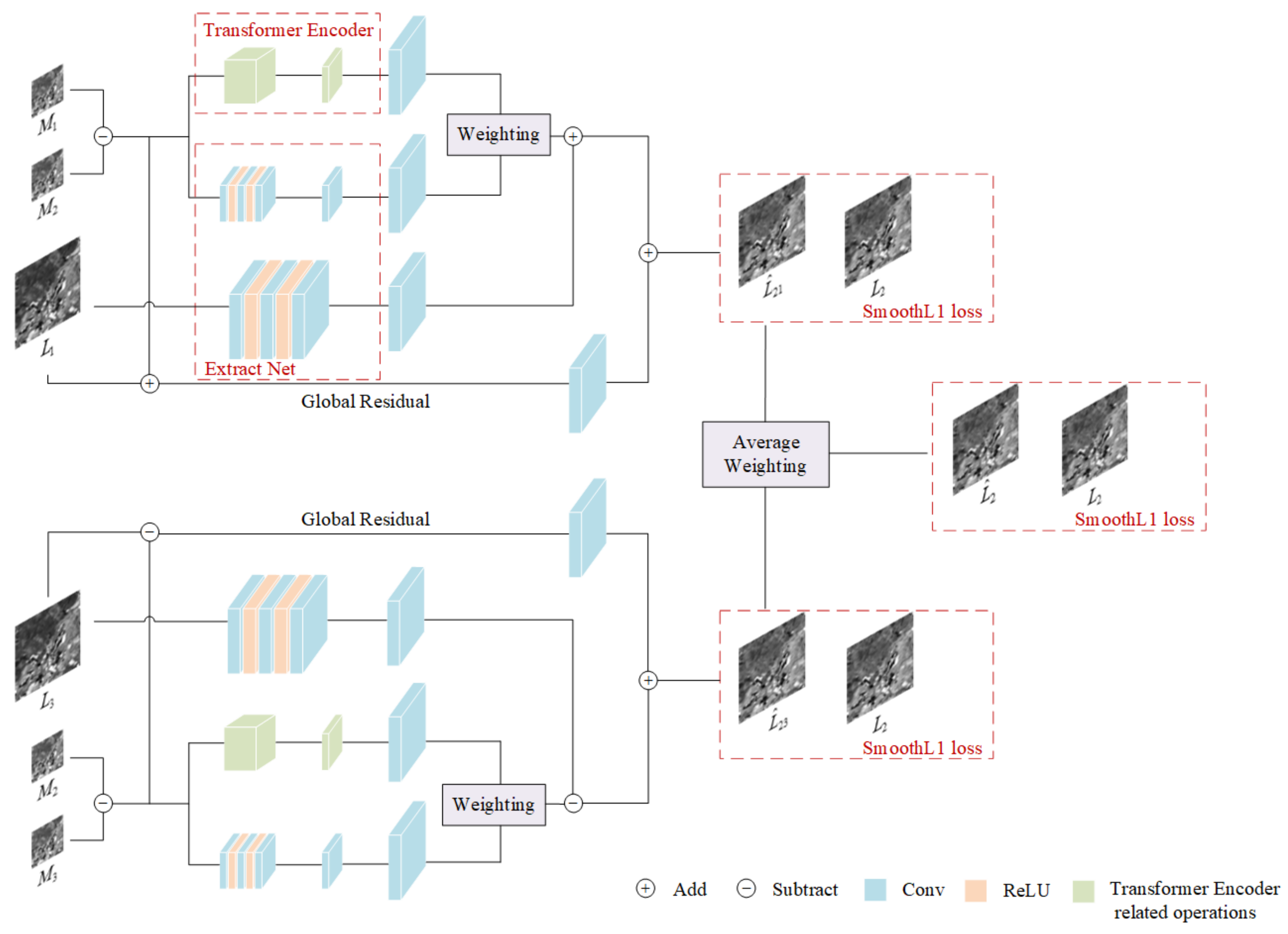
Figure 1 shows the overall structure of MSNet, where $M_i(i=1,2,3)$ represents the MODIS image at time $t_i$, $L_i$ represents the Landsat image at time $t_i$, and ${\hat{L}}_{i(j)}$ represents the prediction result of the fusion image at time $t_i(i=2)$ based on time $t_j(j=1,3)$. Moreover, the three-dimensional blocks of different colours represent different operations, including convolution operations, activation functions ReLU and Transformer encoder, and other related operations.

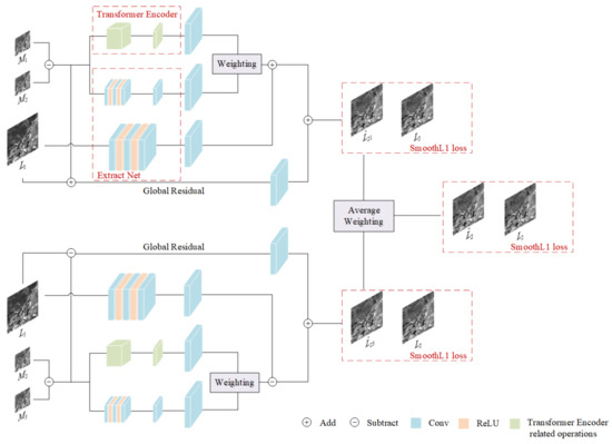
Figure 1. MSNet architecture.

The whole of MSNet is an end-to-end structure, which can be divided into three parts:

• Transformer encoder-related operation modules, which are used to extract time-varying features and learn global temporal correlation information.
• Extract Net, which is used to establish a non-linear mapping relationship between input and output, can extract time information and spatial details of MODIS and Landsat at the same time.
• Average weighting, which uses an averaging strategy to fuse two intermediate prediction maps obtained from different a priori moments to obtain the final prediction map.

The detailed description of each module is presented in Section 3.2, Section 3.3 and Section 3.4.

We use five images of two sizes as input, two MODIS-Landsat image pairs with a priori time $t_j(j=1,3)$, and a MODIS image with prediction time $t_2$. From the structural point of view, MSNet is symmetric from top to bottom. Let us take the structure of the above half as an example to illustrate:

• First, we subtract $M_1$ from $M_2$ to obtain $M_{12}$, which represents the changed area in the time period from $t_1$ to $t_2$ and provides time change information, while $L_1$ provides spatial detail information. After that, we input $M_{12}$ into the Transformer encoder module and the Extract Net module, respectively, to extract time change information, learn global temporal correlation information, and extract time and space features in MODIS images.
• Secondly, because the size of the MODIS image we input is smaller than the size of the Landsat image, to facilitate the subsequent fusion, we use the bilinear interpolation method for up-sampling, and the extracted feature layer is enlarged sixteen-fold to obtain a feature layer with the same size after Landsat processing. Because some of the information we extract and learn using the two modules overlaps, we use the weighting strategy W to assign a weight to the information extracted by the two modules during fusion. The information extracted by the Transformer encoder gives the weight $\alpha$, and Extract Net is $1-\alpha$; we then obtain a fusion of $M_{12}$ feature layers.
• At the same time, we input $L_1$ into Extract Net to extract spatial detail information, and the obtained feature layer is added with the result obtained in the second step to obtain a feature layer fusion.
• As the number of network layers deepens, the time change information and spatial details in the input image are lost. Inspired by the residual connection of ResNet [26], DensNet [27], and STTFN [23], we added global residual learning to supplement the information that may be lost. We upsample the $M_{12}$ obtained in the first step with bilinear interpolation and add it to $L_1$ to obtain a residual learning block. Finally, we add the residual learning block and the result obtained in the third step to obtain a prediction result ${\hat{L}}_{21}$ for the fused image based on time $t_1$ to time $t_2$.

In the same way, the structure of the lower part uses a similar method to obtain the prediction image ${\hat{L}}_{23}$, but it is worth noting that we are predicting the fusion image at time $t_2$. Therefore, in the prediction process of ${\hat{L}}_{23}$, the global residual block is obtained, and the third step of the fusion process is obtained by subtraction.

The structure of the upper and lower parts of MSNet can be expressed using the following formula:

$${\hat{L}}_{21}=E(L_1)+\alpha I(T(M_{12}))+(1-\alpha )I(E(M_{12}))+(L_1+I(M_{12}))$$

(1)

$${\hat{L}}_{23}=E(L_3)-\alpha I(T(M_{23}))-(1-\alpha )I(E(M_{23}))+(L_3-I(M_{23}))$$

(2)

where $T$ represents the related module of the Transformer encoder, $E$ represents Extract Net, $I$ represents the bilinear interpolation upsampling method, and $\alpha =0.4$.

Finally, we obtain two prediction maps ${\hat{L}}_{21}$ and ${\hat{L}}_{23}$, and then reconstruct them using the fusion method of average weighting to obtain the final prediction result ${\hat{L}}_2$ for time $t_2$. The prediction result can be expressed with the following formula:

$${\hat{L}}_2=A({\hat{L}}_{21},{\hat{L}}_{23})$$

(3)

where $A$ represents the average weighting fusion method.

3.2. Transformer Encoder

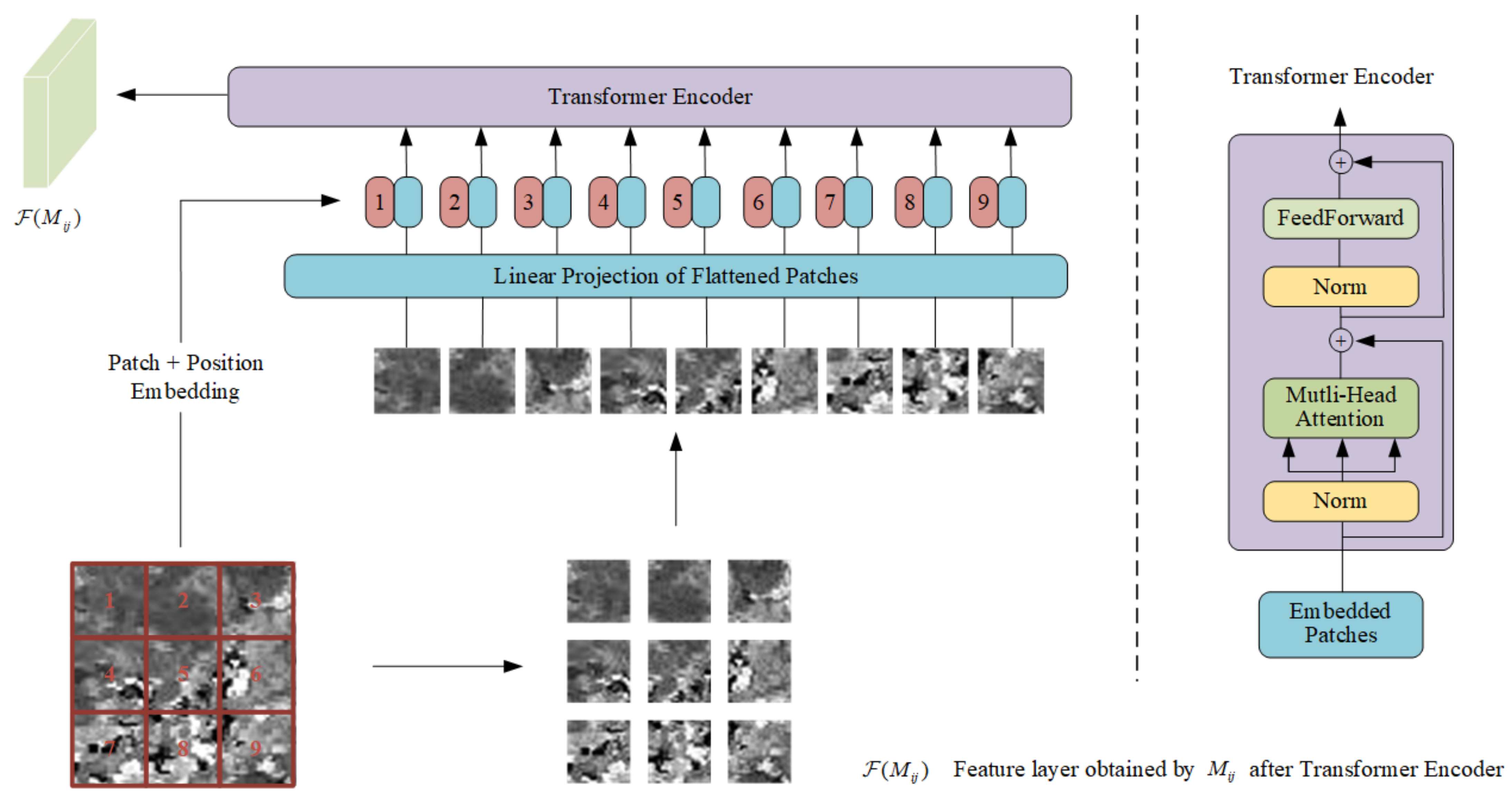
As one applications of the attention mechanism, Transformer [24] is generally used to calculate the correlation degree of the input sequence. It achieves good results not only in natural language processing, but also in applications in the field of vision. For example, Vision Transformer (ViT) [25] partially changed the original Transformer and applied it to image classification. Experiments show that it also has good results. Inspired by the application of Transformer to the attention mechanism and its development in the field of vision, we attempt to apply Transformer to the reconstruction process in spatiotemporal fusion. We selected the Encoder part of Transformer as a module for learning the degree of correlation between blocks in the time change information, that is, the global time correlation information, and it also extracts some of the time change feature information. We refer to the original Transformer and the structural implementation in ViT, and make corresponding changes to obtain the Transformer encoder that can be applied to space–time fusion as shown in Figure 2 below:

Figure 2. Transformer encoder applied to spatiotemporal fusion.

The left part of the dotted line in Figure 2 is the specific process we use for learning. By dividing the input time change information, $M_{12}$, into multiple small patches, and then using a trainable linear projection of flattened patches and mapping it to a new single dimension, this dimension can be used as a constant latent vector in all layers of the Transformer encoder. While the patches are flattened and embedded in the new dimension, the location information from the patches is also embedded in the new dimension as the input of our Transformer encoder. These structures are consistent with ViT. The difference is that we removed the learnable classification embedding in ViT because we don’t need to classify the input. In addition, we also removed the MLP part used to achieve classification in ViT. Through these operations, we ensure that our input and output are of the same dimension, which facilitates our subsequent fusion reconstruction.

The right part of the dotted line in Figure 2 is the specific structure of the Transformer encoder obtained by referring to the original Transformer and ViT. It is composed of a multi-head self-attention mechanism and an alternate feedforward part. The input will be normalized before each input to the submodule, and there will be residual connections after each block. The multi-head self-attention mechanism is a series of Softmax and linear operations. Our input will gradually change its dimensions during the propagation of the training process to adapt to these operations. The feedforward part is composed of linear, Gaussian error linear unit (GELU) and random deactivation dropout, where GELU is used as the activation function. In practical applications, we adjust the number of heads of the multi-head attention mechanism to adapt to different application scenarios. At the same time, for different amounts of data, when global time change information is learned, Transformer encoders of different depths are required to learn more accurately.

Through the above-mentioned position embedding, patch embedding, and self-attention mechanism in the module, we obtain the correlation between the blocks in the time change information and its characteristics during the learning process.

3.3. Extract Net

To extract the temporal and spatial features contained in $M_{ij}$ and the high-frequency spatial detail features in $L_j$, and to establish the mapping relationship between input and prediction results, we propose a five-layer convolutional neural network as our Extract Net, and our input size is different. When extracting different inputs, our convolution kernel size is also different. The size of the Extract Net convolution kernel corresponding to a small input is 3 × 3, and the size for large input is 5 × 5. Different convolution kernel sizes are used to obtain different receptive fields when inputs of different sizes are extracted, thereby enhancing the learning effect [28]. The dimensions of the output feature maps obtained after inputs of different sizes are entered into Extract Net are different, but the feature maps are sampled to the same dimension by upsampling in the follow-up for fusion reconstruction. The structure of Extract Net and receptive field are as shown in Figure 3:

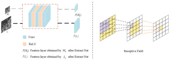
Figure 3. Extract Net.

Specifically, we have a three-layer convolution operation, and there is a rectified linear unit (ReLU) behind the input and hidden layers for activation. For each convolution operation, it can be defined as:

$$\mathsf{\Phi }(x)=w_i\times x+b_i$$

(4)

where $x$ represents the input, “$\times$” represents the convolution operation, $w_i$ represents the weight of the current convolution layer, and $b_i$ represents the current offset. The output channels of the three convolution operations are different, and they are 32, 16, and 1.

After convolution, the ReLU operation makes the feature non-linear and prevents network overfitting [29]. The ReLU operation can be defined as:

$$f(x)=\max (0,\mathsf{\Phi }(x))$$

(5)

We then merge the corresponding feature maps obtained after Extract Net.

3.4. Average Weighting

After the fusion of the Transformer encoder, Extract Net, and the global residuals, two prediction results ${\hat{L}}_{21}$ and ${\hat{L}}_{23}$ for time $t_2$ are obtained. The two prediction results we obtained show some overlap in the process of predicting spatial details and time changes, and our input data is consistent over the time span of the two prior times and the prediction time. Therefore, we use the average weight to obtain the final prediction result, avoiding the use of complex reconstruction methods that introduce noise. Average weighting can be defined as:

$${\hat{L}}_2=\beta {\hat{L}}_{21}+(1-\beta ){\hat{L}}_{23}$$

(6)

where $\beta =0.5$.

3.5. Loss Function

Our method obtains two intermediate prediction results ${\hat{L}}_{21}$ and ${\hat{L}}_{23}$ during the prediction process, as well as the result ${\hat{L}}_2$. During the training process, we perform loss calculations on these three results to continuously adjust during the backpropagation process. The parameters are learned to obtain better convergence results. When each prediction result and its true value are calculated, we choose the smooth L1 loss function, Huber Loss [30], which can be defined as follows:

$$loss({\hat{L}}_{2(j)},L_2)=\frac{1}{N}\left\{\begin{array}{ll}\frac{1}{2}{({\hat{L}}_{2(j)}-L_2)}^2,& if\left|{\hat{L}}_{i(j)}-L_2\right|<1\\ \left|{\hat{L}}_{2(j)}-L_2\right|-\frac{1}{2},& otherwise\end{array}\right.j=1,3$$

(7)

where ${\hat{L}}_{2(j)}$ represents our prediction results ${\hat{L}}_{21}$, ${\hat{L}}_{23}$, ${\hat{L}}_2$, $L_2$ are the real values, and $N$ is our sample size. When the difference between the predicted value and the real value is small, that is, when the difference is between (−1, 1), the square of the result of the subtraction can be used to make the gradient not too large. When the result is large, the calculation method of the absolute value can be used to make the gradient small enough and more stable. Our overall loss function is defined as:

$$\mathcal{L}=loss({\hat{L}}_{21},L_2)+loss({\hat{L}}_{23},L_2)+\lambda loss({\hat{L}}_2,L_2)$$

(8)

where $\lambda =1$. The result of the intermediate prediction is as important as the final prediction. In the experimental comparison, we set the weight $\lambda$ to 1 to enable our model to obtain a better convergence result.

4. Experiment

4.1. Datasets

We used three datasets to test the robustness of MSNet.

The first study area was the Coleambally Irrigation District (CIA) located in the southern part of New South Wales, Australia (NSW, 34.0034°E, 145.0675°S) [31]. This dataset was obtained from October 2001 to May 2002 and contains a total of 17 pairs of MODIS–Landsat images. The Landsat images are all from Landsat-7 ETM+, and the MODIS images are MODIS Terra MOD09GA Collection 5 data. The CIA dataset includes a total of six bands, and the image size is 1720 × 2040.

The second study area is the Lower Gwydir Basin (LGC) located in northern New South Wales, Australia (NSW, 149.2815°E, 29.0855°S) [31]. The dataset was obtained from April 2004 to April 2005 and consists of a total of 14 pairs of MODIS–Landsat images. All the Landsat images are from Landsat-5 TM, and the MODIS images are MODIS Terra MOD09GA Collection 5 data. The LGC dataset contains six bands, and the image size is 3200 × 2720.

The third research area was the Aluhorqin Banner (43.3619°N, 119.0375°E) in the central part of the Inner Mongolia Autonomous Region in northeastern China. This area has many circular pastures and farmland (AHB) [32,33]. Li et al., collected 27 cloudless MODIS–Landsat image pairs from May 2013 to December 2018, a span of more than 5 years. Due to the growth of crops and other types of vegetation, the area showed significant phenological changes. The AHB dataset contains six bands, and the image size is 2480 × 2800.

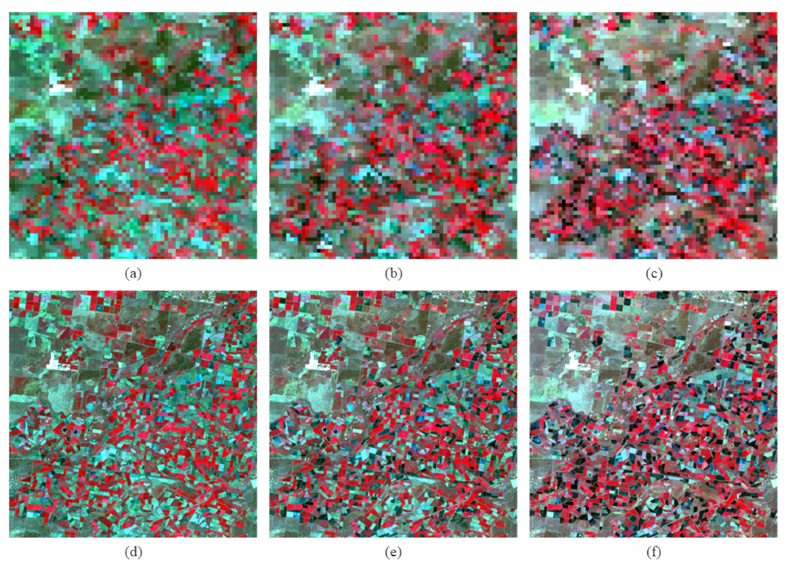
We combined all the images of the three datasets according to two prior moments (letter subscripts are 1 and 3) and an intermediate prediction moment (letter subscript is 2). Each set of training data has six images, including three pairs of MODIS–Landsat images. At the same time, when data were combined, we chose data with the same time span between the prior moment and the predicted moment as our experimental data. In addition, in order to train our network, we first cropped the three datasets to a size of 1200 × 1200. To effectively reduce the increase in the number of parameters due to the deepening of the Transformer encoder, we scaled all the MODIS data to a size of 75 × 75. Figure 4, Figure 5 and Figure 6, respectively, show the MODIS–Landsat image pairs obtained from the three datasets on three different dates. The MODIS data size used for display is 1200 × 1200. Throughout the experiment, we separately input the three datasets into MSNet for training. We use 70% of the dataset for training, 15% for verification, and 15% as a test for our final evaluation of the model’s fusion reconstruction ability.

Figure 4. Composite MODIS (top row) and Landsat (bottom row) image pairs on 7 October (a,d), 16 October (b,e), and 1 November (c,f) 2001 from the CIA [31] dataset. The CIA dataset mainly contains significant phenological changes of irrigated farmland.

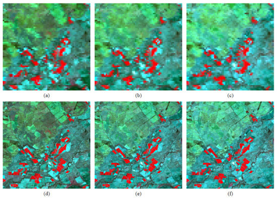
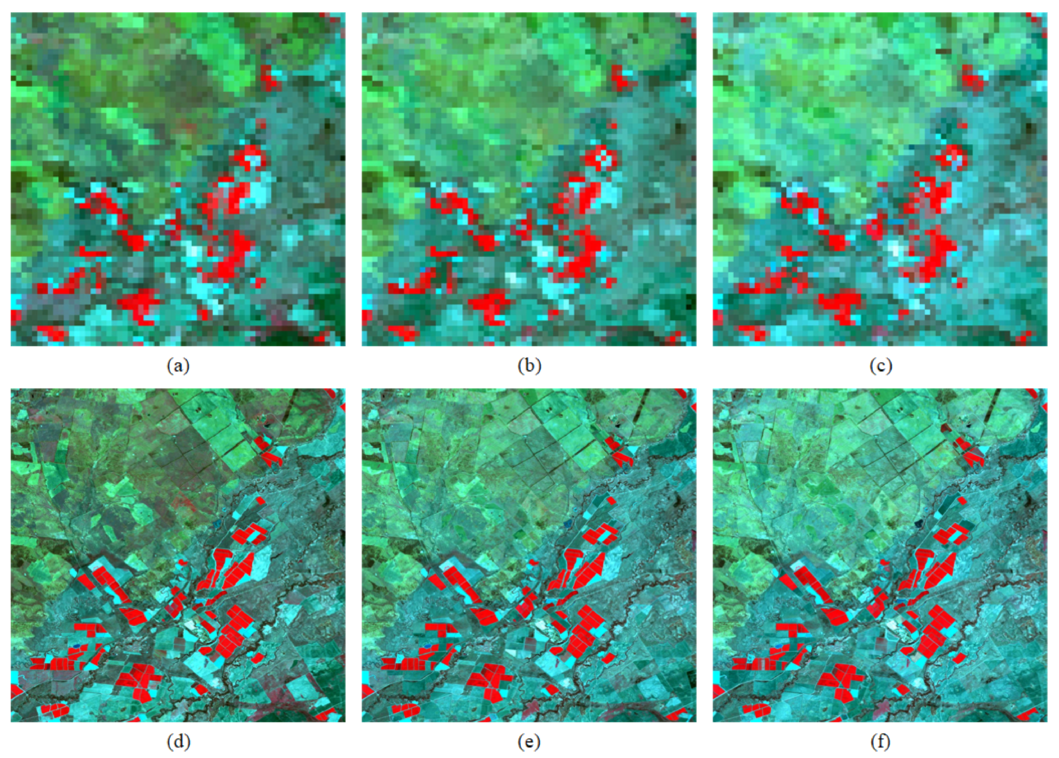
Figure 5. Composite MODIS (top row) and Landsat (bottom row) image pairs on 29 January (a,d), 14 February (b,e), and 2 March (c,f) 2005 from the LGC [31] dataset. The LGC dataset mainly contains changes in land cover types after the flood.

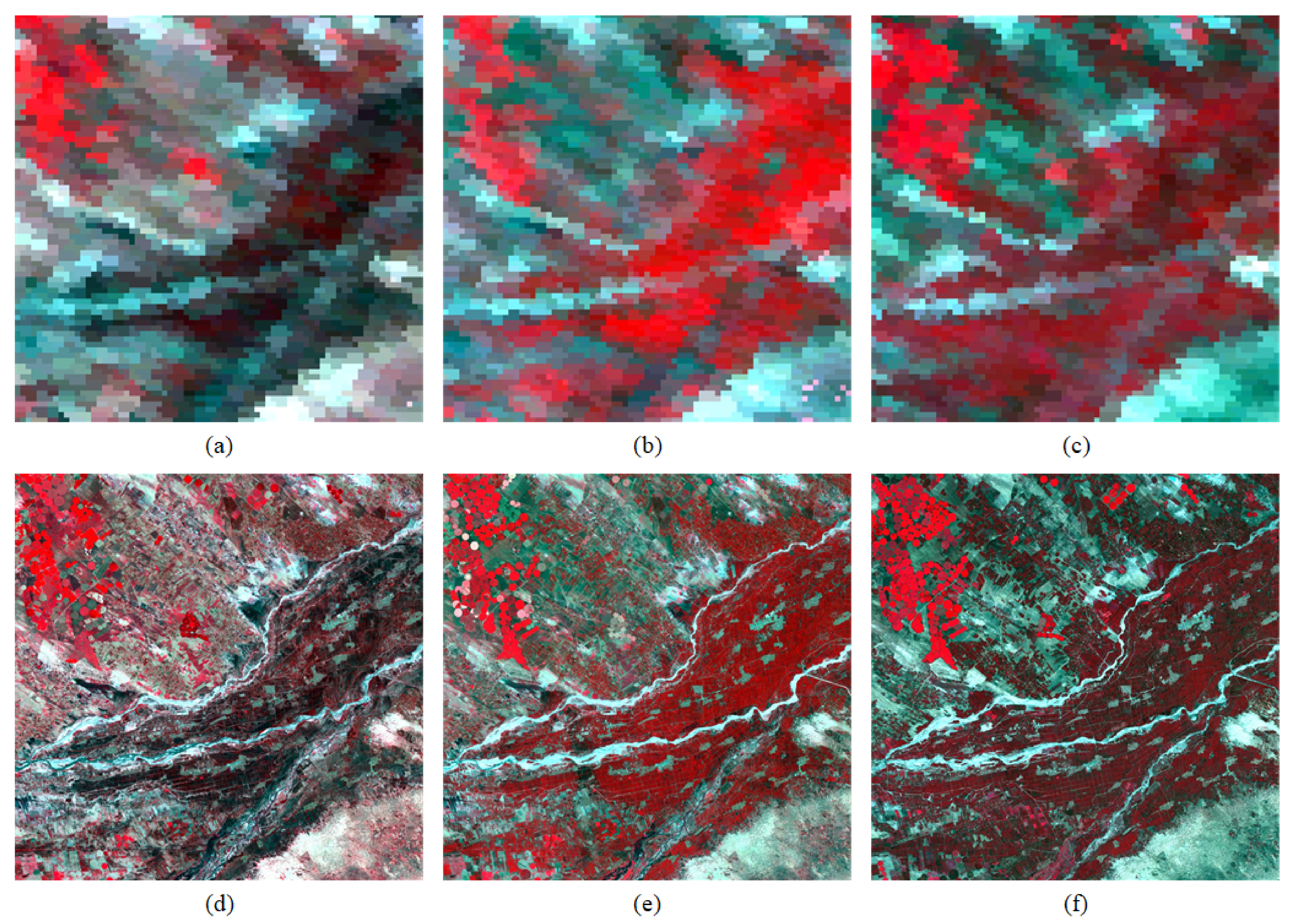
Figure 6. Composite MODIS (top row) and Landsat (bottom row) image pairs on 21 June (a,d), 7 July (b,e), and 25 September (c,f) 2015 from the AHB [32,33] dataset. The AHB dataset mainly contains significant phenological changes of the pasture.

4.2. Evaluation

To evaluate the results of our proposed spatiotemporal fusion method, we compared it with FSDAF, STARFM, STFDCNN and StfNet under the same conditions.

The first indicator we used was the Spectral Angle Mapper (SAM) [34], which measures the spectral distortion of the fusion result. It can be defined as follows:

$$SAM=\frac{1}{N}{\displaystyle \sum _{n=1}^N\arccos }\frac{{\Sigma }_{j=1}^K=(L_i^k{\hat{L}}_i^k)}{\sqrt{{\Sigma }_{j=1}^K{(L_i^k)}^2{\Sigma }_{j=1}^K{({\hat{L}}_i^k)}^2}}$$

(9)

where $N$ represents the total number of pixels in the predicted image, $K$ represents the total number of bands, ${\hat{L}}_i$ represents the prediction result, ${\hat{L}}_i^k$ represents the prediction result of the $k\mathrm{th}$ band, and $L_i^k$ represents the true value of the $L_i^k$ band. A small SAM indicates a better result.

The second metric was the root mean square error (RMSE), which is the square root of the MSE, and is used to measure the deviation between the predicted image and the observed image. It reflects a global depiction of the radiometric differences between the fusion result and the real observation image, which is defined as follows:

$$RMSE=\sqrt{\frac{{\displaystyle \sum _{m=1}^H{\displaystyle \sum _{n=1}^W{\left(L_i(m,n)-{\hat{L}}_i(m,n)\right)}^2}}}{H\times W}}$$

(10)

where $H$ represents the height of the image, $W$ represents the width of the image, $L$ represents the observed image, and ${\hat{L}}_i$ represents the predicted image. The smaller the value of RMSE, the closer the predicted image is to the observed image.

The third indicator was erreur relative global adimensionnelle de synthese (ERGAS) [35], which measures the overall integration result. It can be defined as:

$$ERGAS=100\frac{h}{l}\sqrt{\frac{1}{K}{\displaystyle \sum _{i=1}^K[RMSE{(L_i^k)}^2/{({\mu }_k)}^2]}}$$

(11)

where $h$ and $l$ represent the spatial resolution of Landsat and MODIS images respectively; $L_i^k$ represents the real image of the $k\mathrm{th}$ band; and ${\mu }_k$ represents the average value of the $k\mathrm{th}$ band image. When ERGAS is small, the fusion effect is better.

The fourth index was the structural similarity (SSIM) index [18,36], which is used to measure the similarity of two images. It can be defined as:

$$SSIM=\frac{(2{\mu }_{{\hat{L}}_i}{\mu }_{L_i}+c_1)(2{\sigma }_{{\hat{L}}_i{L}_i}+c_2)}{({\mu }_{{\hat{L}}_i}^2+{\mu }_{L_i}^2+c_1)({\sigma }_{{\hat{L}}_i}^2+{\sigma }_{L_i}^2+c_2)}$$

(12)

where ${\mu }_{{\hat{L}}_i}$ represents the mean value of the predicted image, ${\mu }_{L_i}$ represents the mean value of the real observation image, ${\sigma }_{{\hat{L}}_i{L}_i}$ represents the covariance of the predicted image ${\hat{L}}_i$ and the real observation image $L_i$, ${\sigma }_{{\hat{L}}_i}^2$ represents the variance of the predicted image ${\hat{L}}_i$, ${\sigma }_{L_i}^2$ represents the variance of the real observation image $L_i$, and $c_1$ and $c_2$ are constants used to maintain stability. The value range of SSIM is [−1, 1]. The closer the value is to 1, the more similar are the predicted image and the observed image.

The fifth index is the correlation coefficient (CC), which is used to indicate the correlation between two images. It can be defined as:

$$CC=\frac{{\displaystyle \sum _{n=1}^N({\hat{L}}_i^n-{\mu }_{{\hat{L}}_i})(L_i^n-{\mu }_{L_i})}}{\sqrt{{\displaystyle \sum _{n=1}^N{({\hat{L}}_i^n-{\mu }_{{\hat{L}}_i})}^2}}\sqrt{{\displaystyle \sum _{n=1}^N{(L_i^n-{\mu }_{L_i})}^2}}}$$

(13)

The closer the CC is to 1, the greater the correlation between the predicted image and the real observation image.

The sixth indicator is the peak signal-to-noise ratio (PSNR) [37]. It is defined indirectly by the MSE, which can be defined as:

$$MSE=\frac{1}{HW}{\displaystyle \sum _{m=1}^H{\displaystyle \sum _{n=1}^W{\left(L_i(m,n)-{\hat{L}}_i(m,n)\right)}^2}}$$

(14)

Then PSNR can be defined as:

$$PSNR=10\times {\log }_{10}(\frac{MA{X}_{L_i}^2}{MSE})$$

(15)

where $MA{X}_{L_i}^2$ is the maximum possible pixel value of the real observation image $L_i$. If each pixel is represented by an 8-bit binary value, then $MA{X}_{L_i}$ is 255. Generally, if the pixel value is represented by B-bit binary, then $MA{X}_{L_i}=2^B-1$. PSNR can evaluate the quality of the image after reconstruction. A higher PSNR means that the predicted image quality is better.

4.3. Parameter Setting

For the Transformer encoder, we set the number of headers to nine and set the depth according to the data volume of the three datasets. CIA is 5, LGC is 5, and AHB is 20. The size of the patch is 15 × 15. Different Extract Net sets the size of its convolution kernel to 3 × 3 and 5 × 5. Our initial learning rate is set to 0.0008, the optimizer uses Adam, and the weight attenuation is set to 1e-6. We trained MSNet in a Windows 10 professional environment, equipped with 64 GB RAM, an Intel Core^TM i9–9900K processor running at 3.60 GHz × 16 CPUs, and an NVIDIA GeForce RTX 2080 Ti GPU.

4.4. Results and Analysis

4.4.1. Subjective Evaluation

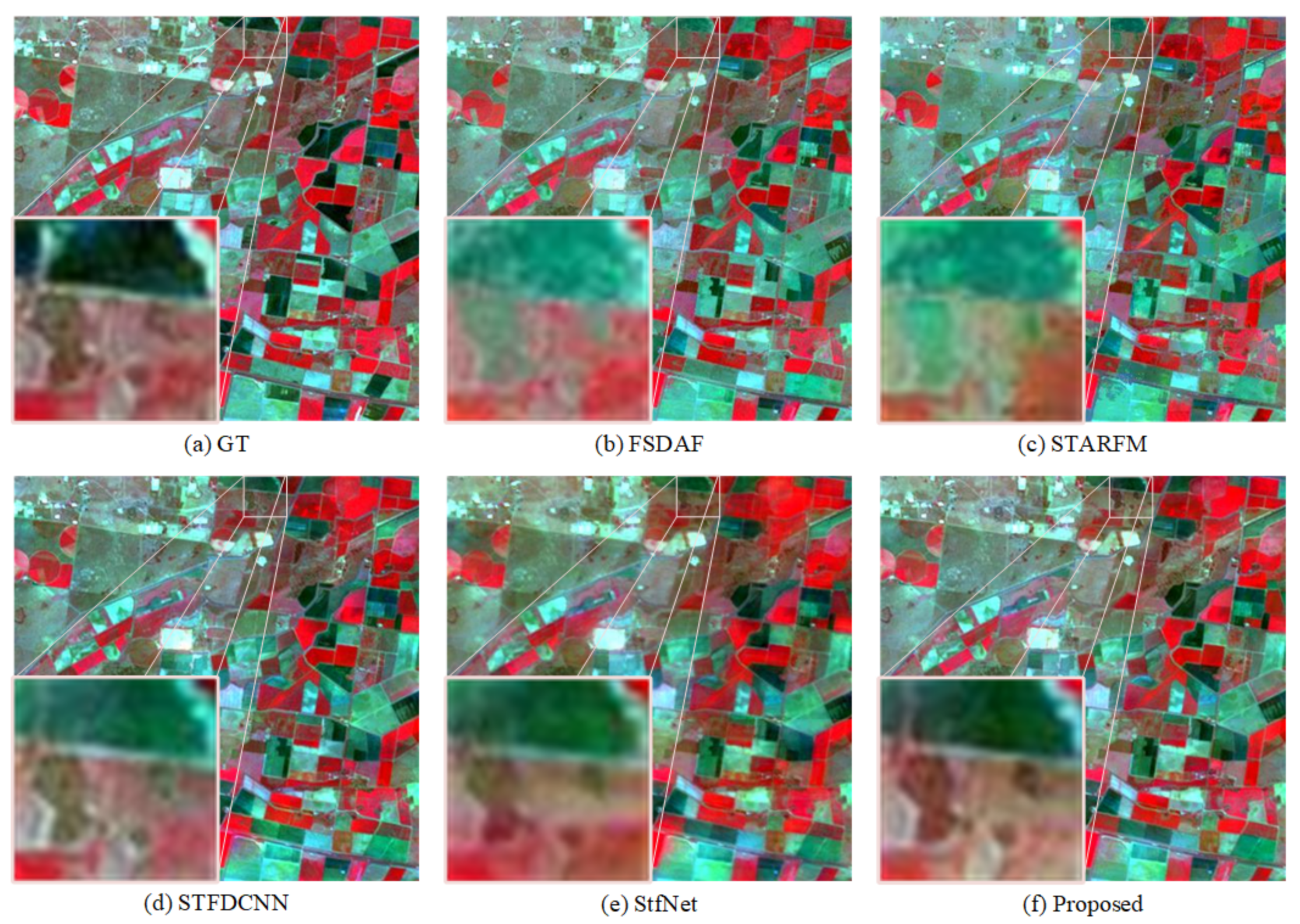
To visually show our experimental results, Figure 7, Figure 8, Figure 9 and Figure 10 respectively show the experimental results of FSDAF [13], STARFM [8], STFDCNN [18], StfNet [19] and our proposed MSNet on the three datasets.

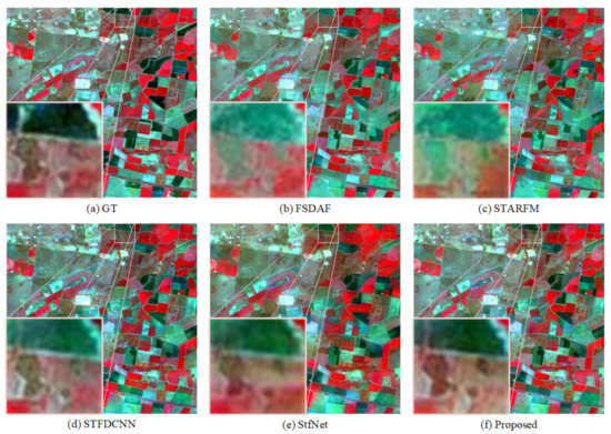
Figure 7. Prediction results for the target Landsat image (16 October 2001) in the CIA [31] dataset. Additionally, comparison methods include FSDAF [13], STARFM [8], STFDCNN [18] and StfNet [19], which are represented by (b–e) in the figure respectively. In addition, (a) represents the ground truth (GT) we got, and (f) represents the method we proposed.

Figure 8. Prediction results for the target Landsat image (14 February 2005) in the LGC [31] dataset. Additionally, comparison methods include FSDAF [13], STARFM [8], STFDCNN [18], and StfNet [19], which are represented by (b–e) in the figure respectively. In addition, (a) represents the ground truth (GT) we got, and (f) represents the method we proposed.

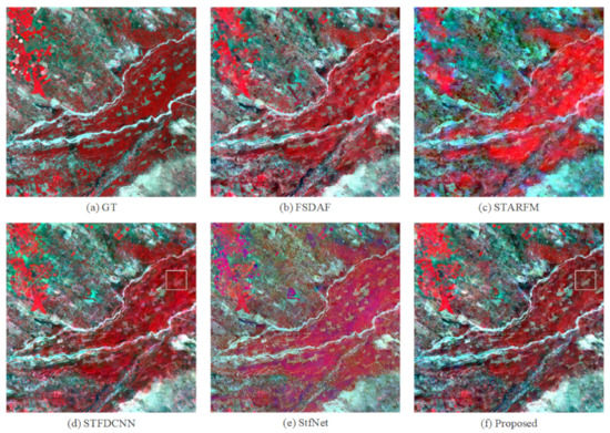
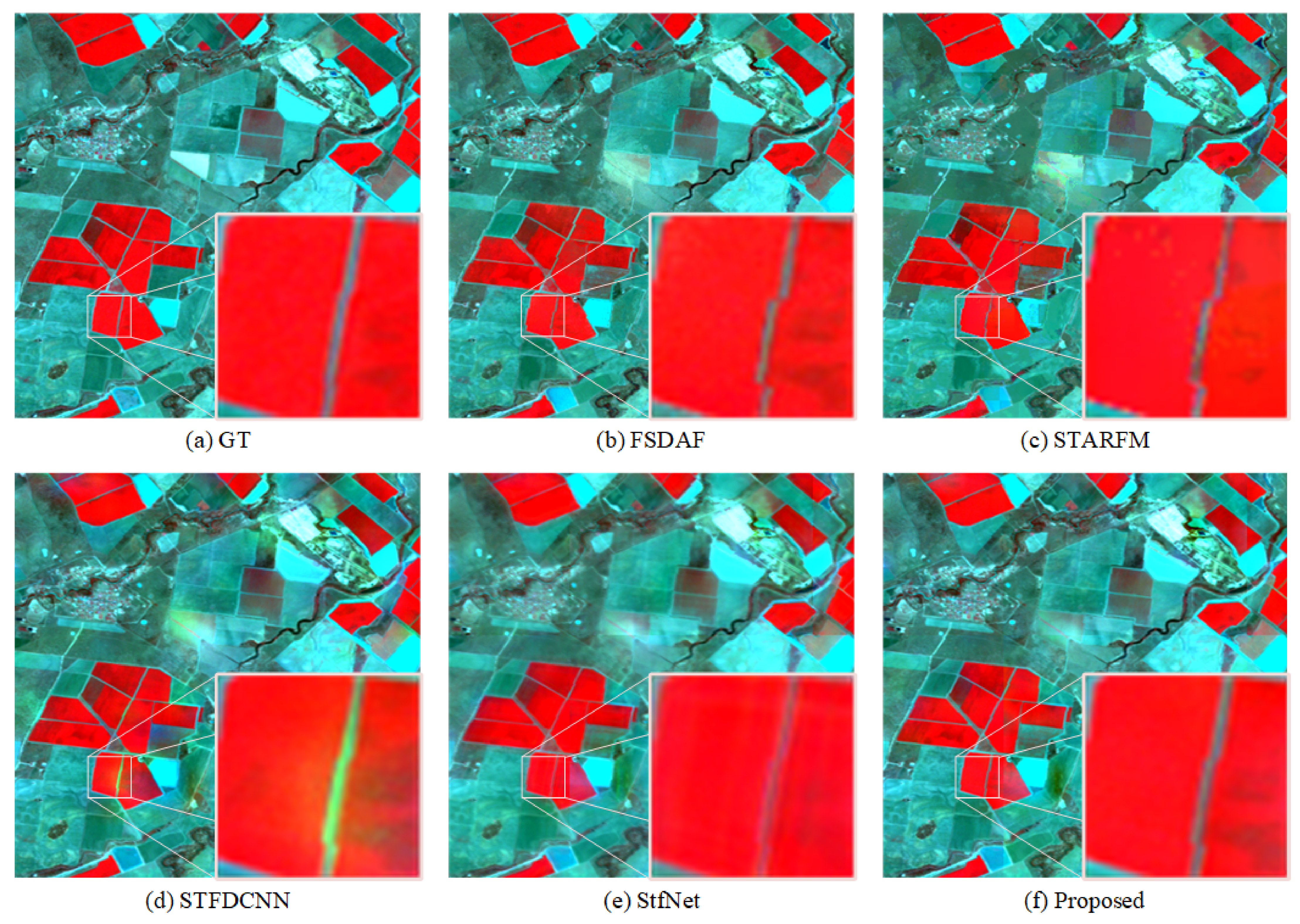
Figure 9. Full prediction results for the target Landsat image (7 July 2015) in the AHB [32,33] dataset. Additionally, comparison methods include FSDAF [13], STARFM [8], STFDCNN [18], and StfNet [19], which are represented by (b–e) in the figure respectively. In addition, (a) represents the ground truth (GT) we got, and (f) represents the method we proposed.

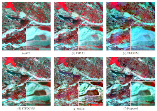
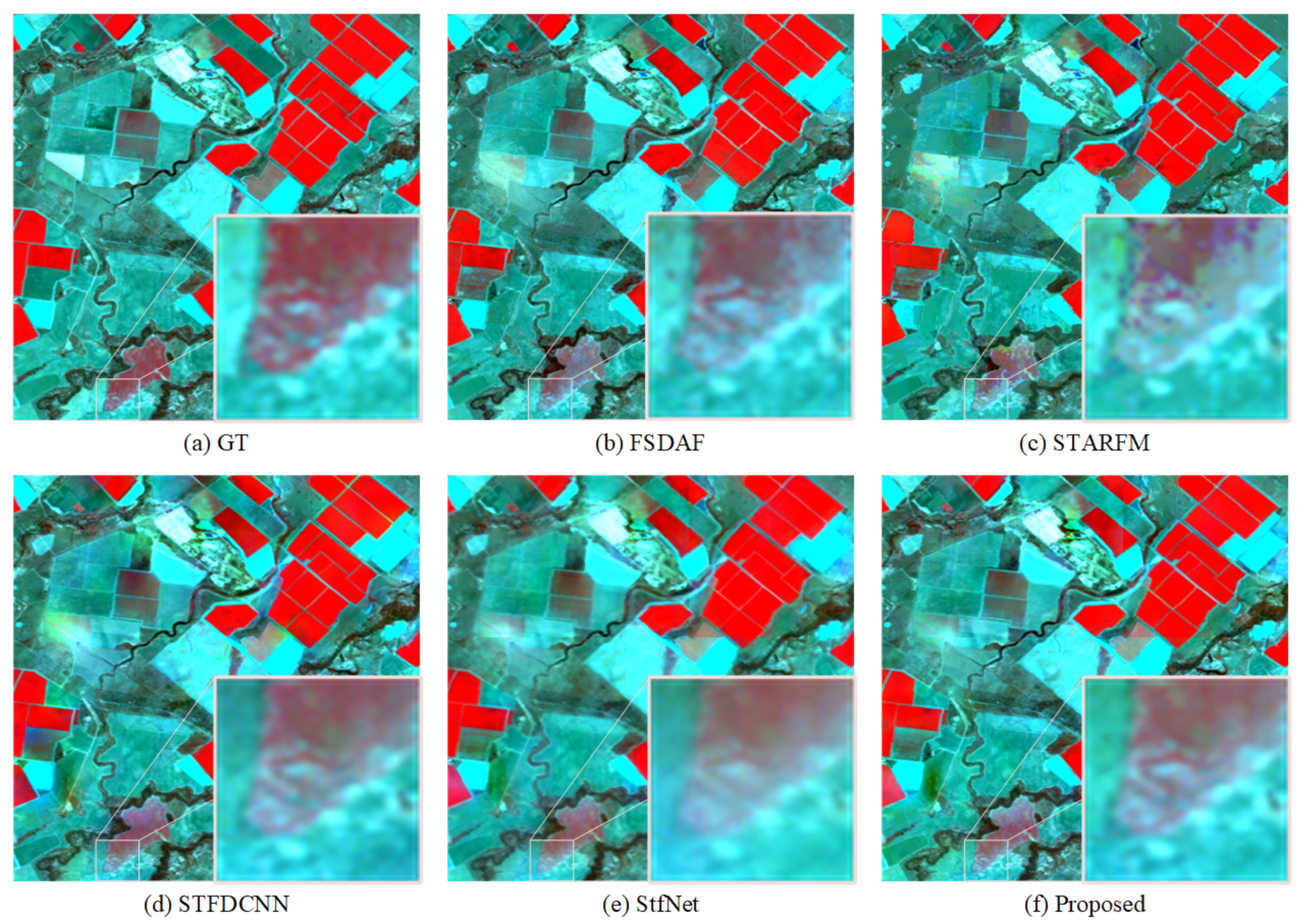
Figure 10. Specific prediction results for the target Landsat image (7 July 2015) in the AHB [32,33] dataset. Additionally, comparison methods include FSDAF [13], STARFM [8], STFDCNN [18], and StfNet [19], which are represented by (b–e) in the figure respectively. In addition, (a) represents the ground truth (GT) we got, and (f) represents the method we proposed.

Figure 7 shows the experimental results we obtained on the CIA dataset. We extracted some of the prediction results for display. “GT” represents the real observation image, and “Proposed” is our MSNet method. In terms of visual effects, FSDAF and STARFM are not accurate enough in predicting phenological changes. For example, there are many land parcels with black areas that cannot be accurately predicted. Relatively speaking, the prediction results obtained by the deep learning method are better, but the prediction map of StfNet is somewhat fuzzy and the result is not good. In addition, we zoom in on some areas for a more detailed display. We can see from the figure that STFDCNN, StfNet and our proposed method achieve better results for the edge processing part of the land. Moreover, the spectral information from the prediction results obtained by MSNet is closer to the true value, as reflected in the depth of the colour, which proves that our prediction results are better.

Figure 8 shows the experimental results we obtained on the LGC dataset. We extracted some of the prediction results for display. Overall, the performance of each algorithm is relatively stable, but there are differences in specific boundary processing and spectral information processing. We zoom in on some areas in the figure to show the details. We can see that the three methods, FSDAF, STARFM, and StfNet, show poor performance in processing high-frequency information in the border area. The boundaries obtained by the prediction results for FSADF and STARFM are not neat enough, and the processing results of StfNet blur the boundary information. In addition, although STFDCNN achieves good results on the boundary information, its spectral information, such as the green part, has not been processed well. In contrast, our proposed method not only achieves the accurate prediction of boundary information, but also shows better processing of spectral information, which is closer to the true value.

Figure 9 and Figure 10 are the full prediction results and the truncated partial results we obtained on the AHB dataset.

From the results in Figure 9, we can see that the prediction results for STARFM are not accurate enough for the processing of spectral information, and there is a large amount of fuzzy spectral information. In addition, although FSDAF’s prediction results are much better than STARFM for the processing of spectral information, they still have shortcomings compared with the true value, such as the insufficient degree of predicted phenological changes, which is reflected in the difference in colour. StfNet shows good results for most predictions, such as the spatial details between rivers. However, it can also be seen that there are still shortcomings in the prediction of time information, and the phenological change information in some areas is not accurately predicted. The performance of STFDCNN and our proposed method is better in terms of time information. However, in the continuous phenological change area, STFDCNN’s prediction results are not good. For example, in rectangular area in the figure, its prediction result is not good. In contrast, our proposed method achieves better results.

Figure 10 shows the details after we zoomed in on the prediction results. For small, raised shoals in the river, neither FSDAF nor STARFM can accurately predict the edge in-formation and the time information it should contain, and the prediction result is not good. Although STFDCNN and StfNet have relatively perfect spatial information pro-cessing and clear boundaries, the spectral information is still quite different from the true value. Compared with our method, our results are more accurate in the processing of spa-tial information and spectral information and are closer to the true value.

4.4.2. Objective Evaluation

To objectively evaluate our proposed algorithm, we used six evaluation indicators to evaluate various algorithms and our MSNet. Table 2, Table 3 and Table 4 show our quantitative evaluation of the prediction results obtained by various methods on three datasets, including the global indicators SAM and ERGAS, and the local indicators RMSE, SSIM, PSNR, and CC. In addition, we also boldly mark the optimal value of each indicator.

Table 2. Quantitative assessment of different spatiotemporal fusion methods for the CIA [31] dataset.

Evaluation	Band	Method
		FSDAF [13]	STARFM [8]	STFDCNN [18]	StfNet [19]	Proposed
SAM	all	0.23875	0.23556	0.21402	0.21614	0.19209
ERGAS	all	3.35044	3.31676	3.14461	3.00404	2.94471
RMSE	band1	0.01365	0.01306	0.01076	0.00956	0.01009
	band2	0.01415	0.01366	0.01236	0.01271	0.01132
	band3	0.02075	0.02055	0.01792	0.02121	0.01724
	band4	0.04619	0.04899	0.04100	0.05001	0.03669
	band5	0.06031	0.06153	0.05900	0.05302	0.04898
	band6	0.05322	0.05278	0.05389	0.04500	0.04325
	avg	0.03471	0.03509	0.03249	0.03192	0.02793
SSIM	band1	0.90147	0.91699	0.95517	0.94190	0.95050
	band2	0.91899	0.92325	0.93812	0.94340	0.95149
	band3	0.85786	0.86290	0.87329	0.89950	0.91156
	band4	0.76070	0.74636	0.78318	0.84868	0.86248
	band5	0.66598	0.66011	0.72789	0.74118	0.76460
	band6	0.66168	0.66323	0.73555	0.74068	0.76257
	avg	0.79445	0.79548	0.83553	0.85256	0.86720
PSNR	band1	37.29537	37.68327	39.36680	40.38939	39.92510
	band2	36.98507	37.29114	38.16128	37.91972	38.92643
	band3	33.65821	33.74247	34.93560	33.46842	35.27141
	band4	26.70854	26.19858	27.74355	26.01829	28.70879
	band5	24.39249	24.21822	24.58366	25.51175	26.19920
	band6	25.47784	25.55050	25.37055	26.93525	27.28095
	avg	30.75292	30.78070	31.69357	31.70714	32.71865
CC	band1	0.80138	0.79845	0.84521	0.83428	0.84448
	band2	0.79873	0.79319	0.83720	0.83156	0.84929
	band3	0.83290	0.82554	0.87373	0.87264	0.87787
	band4	0.88511	0.86697	0.91181	0.90546	0.92743
	band5	0.76395	0.74894	0.78783	0.84732	0.84784
	band6	0.76036	0.75144	0.76502	0.84588	0.83826
	avg	0.80707	0.79742	0.83680	0.85619	0.86420

Table 3. Quantitative assessment of different spatiotemporal fusion methods for the LGC [31] dataset.

Evaluation	Band	Method
		FSDAF [13]	STARFM [8]	STFDCNN [18]	StfNet [19]	Proposed
SAM	all	0.08411	0.08601	0.06792	0.09284	0.06335
ERGAS	all	1.93861	1.92273	1.80392	2.03970	1.68639
RMSE	band1	0.00763	0.00729	0.00719	0.00824	0.00585
	band2	0.00913	0.00907	0.00843	0.01167	0.00712
	band3	0.01279	0.01256	0.01151	0.01353	0.00969
	band4	0.02383	0.02295	0.02102	0.02971	0.01864
	band5	0.02830	0.02607	0.02251	0.02284	0.02159
	band6	0.02197	0.02181	0.01673	0.02054	0.01425
	avg	0.01727	0.01662	0.01457	0.01775	0.01286
SSIM	band1	0.97422	0.97355	0.98460	0.97464	0.98558
	band2	0.96698	0.96495	0.98209	0.96062	0.98031
	band3	0.94456	0.94152	0.97475	0.94162	0.96954
	band4	0.92411	0.91759	0.96417	0.91455	0.96393
	band5	0.89418	0.88558	0.95539	0.91215	0.95239
	band6	0.88485	0.87789	0.95259	0.90154	0.95087
	avg	0.93148	0.92684	0.96893	0.93419	0.96710
PSNR	band1	42.35483	42.73997	42.86245	41.68016	44.65345
	band2	40.79034	40.85222	41.48586	38.65611	42.95050
	band3	37.86428	38.02099	38.77733	37.37629	40.27059
	band4	32.45760	32.78532	33.54859	30.54336	34.59058
	band5	30.96416	31.67671	32.95179	32.82613	33.31671
	band6	33.16535	33.22812	35.52920	33.74927	36.92082
	avg	36.26610	36.55056	37.52587	35.80522	38.78378
CC	band1	0.93627	0.92935	0.94611	0.94664	0.96138
	band2	0.93186	0.92880	0.94530	0.93566	0.95800
	band3	0.93549	0.93516	0.95262	0.95539	0.96499
	band4	0.96360	0.96287	0.97181	0.96125	0.97591
	band5	0.95527	0.95222	0.97545	0.97048	0.97890
	band6	0.95313	0.95214	0.97285	0.97164	0.97924
	avg	0.94594	0.94342	0.96069	0.95684	0.96974

Table 4. Quantitative assessment of different spatiotemporal fusion methods for the AHB [32,33] dataset.

Evaluation	Band	Method
		FSDAF [13]	STARFM [8]	STFDCNN [18]	StfNet [19]	Proposed
SAM	all	0.16991	0.29277	0.18583	0.25117	0.14677
ERGAS	all	2.80156	4.46147	4.25224	3.86535	2.90661
RMSE	band1	0.00039	0.00251	0.00096	0.00112	0.00047
	band2	0.00044	0.00235	0.00092	0.00081	0.00051
	band3	0.00067	0.00358	0.00117	0.00118	0.00064
	band4	0.00109	0.00590	0.00124	0.00201	0.00103
	band5	0.00126	0.00408	0.00183	0.00177	0.00122
	band6	0.00136	0.00263	0.00200	0.00198	0.00126
	avg	0.00087	0.00351	0.00135	0.00148	0.00085
SSIM	band1	0.99895	0.96538	0.99205	0.98927	0.99822
	band2	0.99877	0.96977	0.99293	0.99500	0.99805
	band3	0.99741	0.93438	0.98947	0.98965	0.99740
	band4	0.99616	0.92038	0.99419	0.98248	0.99631
	band5	0.99382	0.94190	0.98371	0.98464	0.99388
	band6	0.99129	0.96825	0.97625	0.97636	0.99226
	avg	0.99607	0.95001	0.98810	0.98623	0.99602
PSNR	band1	68.18177	52.01008	60.34502	59.00582	66.48249
	band2	67.04371	52.56484	60.68929	61.83160	65.80339
	band3	63.49068	48.93197	58.63694	58.55977	63.88021
	band4	59.22553	44.58211	58.13169	53.95486	59.77506
	band5	58.02282	47.79106	54.74701	55.05539	58.28599
	band6	57.35352	51.60634	53.96601	54.06602	58.02322
	avg	62.21967	49.58107	57.75266	57.07891	62.04173
CC	band1	0.84000	0.71181	0.80368	0.49726	0.86845
	band2	0.85657	0.74545	0.86845	0.38062	0.89114
	band3	0.84979	0.81230	0.83576	0.27147	0.88345
	band4	0.53986	0.34009	0.58944	0.37556	0.60303
	band5	0.79576	0.76553	0.83580	0.62926	0.85320
	band6	0.80288	0.76492	0.80338	0.61085	0.85154
	avg	0.78081	0.69002	0.78942	0.46083	0.82514

Table 2 shows the quantitative evaluation results of the multiple fusion methods and our MSNet on the CIA dataset. We achieved optimal values on the global indicators and most of the local indicators.

Table 3 shows the evaluation results of various methods on the LGC dataset. Although our method does not achieve the optimal value for the SSIM evaluation, its value is similar and it achieves the optimal value for the global index and most of the other local indexes.

Table 4 lists the evaluation results of various methods on the AHB dataset. It can be seen that, except for some fluctuations in the evaluation results for individual bands, our method achieves the best values in the rest of the evaluation results.

5. Discussion

From the experiments on three datasets, we can see that our method obtained better forecasting results, both on the CIA dataset with phenological changes in regular areas, and on the AHB dataset with many phenological changes in irregular areas. Similarly, for the LGC dataset, which contains mainly land cover type change, our method achieved better prediction results for the processing of time information than the traditional method and the other two methods based on deep learning. The processing of time information benefits from the use of the Transformer encoder and convolutional neural network in MSNet. More importantly, the Transformer encoder we introduced learns the connection between the local and the global information and better grasps the global temporal information. It is worth noting that for datasets with different data volumes, the depth of the Transformer encoder should also be different to better adapt to the datasets. Table 5 lists the average evaluation values for the prediction results obtained without the introduction of the Transformer encoder and for Transformer encoders having different depths. When no Transformer encoder is introduced, the experimental results are relatively poor. With the changes in the depth of the Transformer encoder, we also obtained different results. When the depth is 5 on the CIA dataset, 5 on the LGC dataset, and 20 on the AHB dataset, we have also achieved better results, and they were better than when only the convolutional neural networks were used.

Table 5. Average evaluation values of Transformer encoders of different depths on the three datasets.

Datasets	Depth	SAM	ERGAS	RMSE	SSIM	PSNR	CC
CIA	0	0.19561	3.04052	0.02869	0.86004	32.47545	0.86223
	5	0.19209	2.94471	0.02793	0.86720	32.71865	0.86420
	10	0.19799	3.02700	0.02879	0.86082	32.42599	0.85658
	15	0.19881	3.00321	0.02875	0.86301	32.41008	0.85536
	20	0.20009	2.96461	0.02883	0.85894	32.49450	0.85069
LGC	0	0.06397	1.70489	0.01282	0.96487	38.73680	0.96823
	5	0.06335	1.68639	0.01286	0.96710	38.78378	0.96974
	10	0.06706	1.72469	0.01333	0.96557	38.47550	0.96499
	15	0.06797	1.76038	0.01350	0.96639	38.11193	0.96243
	20	0.06675	1.74121	0.01340	0.96665	38.21371	0.96467
AHB	0	0.14679	3.10283	0.00089	0.99558	61.37776	0.82436
	5	0.14836	3.13212	0.00094	0.99506	61.07734	0.82328
	10	0.15712	3.21723	0.00097	0.99472	60.71349	0.80382
	15	0.15101	3.12097	0.00093	0.99522	61.01998	0.81928
	20	0.14677	2.90661	0.00085	0.99602	62.04173	0.82514

In addition, Extract Nets with different receptive field sizes have different sizes of learning areas, which effectively adapt to different sizes of input and obtain better results for learning time change information and spatial detail information. Table 6 lists the average evaluation values of the prediction results of Extract Net with different receptive fields. If an Extract Net with a single receptive field size is used for different sizes of input, the result is poor.

Table 6. Average evaluation values of Extract Nets with different sizes of receptive fields on the three datasets.

Datasets	Size	SAM	ERGAS	RMSE	SSIM	PSNR	CC
CIA	3 × 3, 3 × 3	0.20058	2.97356	0.02900	0.85794	32.41488	0.84958
	5 × 5, 5 × 5	0.20175	2.96925	0.02894	0.86145	32.35826	0.84900
	3 × 3, 5 × 5	0.19209	2.94471	0.02793	0.86720	32.71865	0.86420
LGC	3 × 3, 3 × 3	0.07320	1.82552	0.01497	0.96084	37.44287	0.95675
	5 × 5, 5 × 5	0.07127	1.83538	0.01443	0.96422	37.36025	0.95671
	3 × 3, 5 × 5	0.06335	1.68639	0.01286	0.96710	38.78378	0.96974
AHB	3 × 3, 3 × 3	0.19604	3.55414	0.00113	0.9934	59.58018	0.73684
	5 × 5, 5 × 5	0.21244	3.57996	0.00125	0.99244	59.00303	0.67548
	3 × 3, 5 × 5	0.14677	2.90661	0.00085	0.99602	62.04173	0.82514

When the result is obtained through the fusion of two intermediate prediction results, the average weight method obtains a better result in processing some of the noise. We compared the results obtained by the fusion method in STFDCNN [18], and we call this fusion method TC weighting. Table 7 lists the average measured values of the prediction results obtained using different fusion methods. The fusion method that uses the averaging strategy is the correct choice.

Table 7. Average evaluation values of MSNet using different fusion methods on the three datasets.

Datasets	Weighting	SAM	ERGAS	RMSE	SSIM	PSNR	CC
CIA	TC	0.20046	3.02157	0.02917	0.85953	32.29681	0.85509
	Avg	0.19209	2.94471	0.02793	0.86720	32.71865	0.86420
LGC	TC	0.07129	1.79503	0.01444	0.96404	37.73562	0.95589
	Avg	0.06335	1.68639	0.01286	0.96710	38.78378	0.96974
AHB	TC	0.16715	3.20845	0.00097	0.99464	60.64426	0.77796
	Avg	0.14677	2.90661	0.00085	0.99602	62.04173	0.82514

Although the method we proposed has achieved good results overall, there are some shortcomings in some areas. Figure 11 shows the deficiencies in the prediction of phenological change information obtained by each method in the LGC dataset. Compared with the true value, the shortcomings of each prediction result are reflected in the shade of the colour. In this regard, we analysed that this is because our method may not be easy to extract all the information contained in the small change area when focusing on the global temporal correlation. In addition, there are some points worthy of further discussion in our method. First, to reduce the number of parameters, we used the professional remote sensing image processing software ENVI to change the size of the MODIS data, but whether there was a loss of temporal information during this process requires further research to determine. Secondly, the introduction of the Transformer encoder increases the number of parameters. In addition to changing the size of the input, other methods that can reduce the number of parameters and maintain the fusion effect need to be studied in the future. Furthermore, the fusion method for improving the fusion result and avoiding the introduction of noise also needs to be studied further.

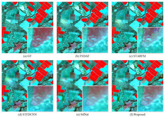
Figure 11. Insufficient prediction results for the target Landsat image (14 February 2005) in the LGC [31] dataset. Additionally, comparison methods include FSDAF [13], STARFM [8], STFDCNN [18], and StfNet [19], which are represented by (b–e) in the figure respectively. In addition, (a) represents the ground truth (GT) we got, and (f) represents the method we proposed.

6. Conclusions

We use data from three research areas to evaluate the effectiveness of our proposed MSNet method and prove that our model is robust. The superior performance of MSNet compared with that of other methods is mainly because:

• The Transformer encoder module is used to learn global time change information. While extracting local features, it uses the self-attention mechanism and the embedding of position information to learn the relationship between local and global information, which is different from the effect of only using the convolution operation. In the end, our method achieves the desired result.
• We set up Extract Net with different convolution kernel sizes to extract the features contained in inputs of different sizes. The larger the convolution kernel, the larger the receptive field. When a larger-sized Landsat image is extracted, a large receptive field can obtain more learning content and achieve better learning results. At the same time, a small receptive field can better match the size of our time-varying information.
• For the repeated extraction of information, we added a weighting strategy when we fused the feature layer obtained and reconstructed the result from the intermediate prediction results to eliminate the noise introduced by the repeated information in the fusion process.
• When we established the complex nonlinear mapping relationship between the input and the final fusion result, we added a global residual connection for learning, thereby supplementing some of the details lost in the training process.

Our experiments showed that in the CIA and AHB datasets, which contain significant phenological changes, and in the LGC dataset with changes in land cover types, our proposed model MSNet was better than other models that use two or three pairs of original images to fuse. The prediction results on each dataset were relatively stable.

References

- Justice, C.O.; Vermote, E.; Townshend, J.R.; Defries, R.; Roy, D.P.; Hall, D.K.; Salomonson, V.V.; Privette, J.L.; Riggs, G.; Strahler, A.; et al. The Moderate Resolution Imaging Spectroradiometer (MODIS): Land remote sensing for global change research. IEEE Trans. Geosci. Remote Sens. 1998, 36, 1228–1249. [Google Scholar] [CrossRef] [Green Version]
- Lin, C.; Li, Y.; Yuan, Z.; Lau, A.K.; Li, C.; Fung, J.C. Using satellite remote sensing data to estimate the high-resolution distribution of ground-level PM2.5. Remote Sens. Environ. 2015, 156, 117–128. [Google Scholar] [CrossRef]
- Zhang, L.; Zhang, Q.; Du, B.; Huang, X.; Tang, Y.Y.; Tao, D. Simultaneous spectral-spatial feature selection and extraction for hyperspectral images. IEEE Trans. Cybern. 2016, 48, 16–28. [Google Scholar] [CrossRef] [Green Version]
- Yu, Q.; Gong, P.; Clinton, N.; Biging, G.; Kelly, M.; Schirokauer, D. Object-based detailed vegetation classification with airborne high spatial resolution remote sensing imagery. Photogramm. Eng. Remote Sens. 2006, 72, 799–811. [Google Scholar] [CrossRef] [Green Version]
- White, M.A.; Nemani, R.R. Real-time monitoring and short-term forecasting of land surface phenology. Remote Sens. Environ. 2006, 104, 43–49. [Google Scholar] [CrossRef]
- Hansen, M.C.; Loveland, T.R. A review of large area monitoring of land cover change using Landsat data. Remote Sens. Environ. 2012, 122, 66–74. [Google Scholar] [CrossRef]
- Gao, F.; Masek, J.; Schwaller, M.; Hall, F. On the blending of the Landsat and MODIS surface reflectance: Predicting daily Landsat surface reflectance. IEEE Trans. Geosci. Remote Sens. 2006, 44, 2207–2218. [Google Scholar] [CrossRef]
- Hilker, T.; Wulder, M.A.; Coops, N.C.; Seitz, N.; White, J.C.; Gao, F.; Masek, J.G.; Stenhouse, G. Generation of dense time series synthetic Landsat data through data blending with MODIS using a spatial and temporal adaptive reflectance fusion model. Remote Sens. Environ. 2009, 113, 1988–1999. [Google Scholar] [CrossRef]
- Zhu, X.; Chen, J.; Gao, F.; Chen, X.; Masek, J.G. An enhanced spatial and temporal adaptive reflectance fusion model for complex heterogeneous regions. Remote Sens. Environ. 2010, 114, 2610–2623. [Google Scholar] [CrossRef]
- Hilker, T.; Wulder, M.A.; Coops, N.C.; Linke, J.; McDermid, G.; Masek, J.G.; Gao, F.; White, J.C. A new data fusion model for high spatial-and temporal-resolution mapping of forest disturbance based on Landsat and MODIS. Remote Sens. Environ. 2009, 113, 1613–1627. [Google Scholar] [CrossRef]
- Zhukov, B.; Oertel, D.; Lanzl, F.; Reinhackel, G. Unmixing-based multisensor multiresolution image fusion. IEEE Trans. Geosci. Remote Sens. 1999, 37, 1212–1226. [Google Scholar] [CrossRef]
- Wu, M.; Niu, Z.; Wang, C.; Wu, C.; Wang, L. Use of MODIS and Landsat time series data to generate high-resolution temporal synthetic Landsat data using a spatial and temporal reflectance fusion model. J. Appl. Remote Sens. 2012, 6, 063507. [Google Scholar] [CrossRef]
- Zhu, X.; Helmer, E.H.; Gao, F.; Liu, D.; Chen, J.; Lefsky, M.A. A flexible spatiotemporal method for fusing satellite images with different resolutions. Remote Sens. Environ. 2016, 172, 165–177. [Google Scholar] [CrossRef]
- Huang, B.; Song, H. Spatiotemporal reflectance fusion via sparse representation. IEEE Trans. Geosci. Remote Sens. 2012, 50, 3707–3716. [Google Scholar] [CrossRef]
- Belgiu, M.; Stein, A. Spatiotemporal image fusion in remote sensing. Remote Sens. 2019, 11, 818. [Google Scholar] [CrossRef] [Green Version]
- Wei, J.; Wang, L.; Liu, P.; Chen, X.; Li, W.; Zomaya, A.Y. Spatiotemporal fusion of MODIS and Landsat-7 reflectance images via compressed sensing. IEEE Trans. Geosci. Remote Sens. 2017, 55, 7126–7139. [Google Scholar] [CrossRef]
- Liu, X.; Deng, C.; Wang, S.; Huang, G.-B.; Zhao, B.; Lauren, P. Fast and accurate spatiotemporal fusion based upon extreme learning machine. IEEE Geosci. Remote Sens. Lett. 2016, 13, 2039–2043. [Google Scholar] [CrossRef]
- Song, H.; Liu, Q.; Wang, G.; Hang, R.; Huang, B. Spatiotemporal satellite image fusion using deep convolutional neural networks. IEEE J. Sel. Top. Appl. Earth Obs. Remote Sens. 2018, 11, 821–829. [Google Scholar] [CrossRef]
- Liu, X.; Deng, C.; Chanussot, J.; Hong, D.; Zhao, B. StfNet: A two-stream convolutional neural network for spatiotemporal image fusion. IEEE Trans. Geosci. Remote Sens. 2019, 57, 6552–6564. [Google Scholar] [CrossRef]
- Tan, Z.; Yue, P.; Di, L.; Tang, J. Deriving high spatiotemporal remote sensing images using deep convolutional network. Remote Sens. 2018, 10, 1066. [Google Scholar] [CrossRef] [Green Version]
- Tan, Z.; Di, L.; Zhang, M.; Guo, L.; Gao, M. An enhanced deep convolutional model for spatiotemporal image fusion. Remote Sens. 2019, 11, 2898. [Google Scholar] [CrossRef] [Green Version]
- Chen, J.; Wang, L.; Feng, R.; Liu, P.; Han, W.; Chen, X. CycleGAN-STF: Spatiotemporal fusion via CycleGAN-based image generation. IEEE Trans. Geosci. Remote Sens. 2020, 59, 5851–5865. [Google Scholar] [CrossRef]
- Yin, Z.; Wu, P.; Foody, G.M.; Wu, Y.; Liu, Z.; Du, Y.; Ling, F. Spatiotemporal fusion of land surface temperature based on a convolutional neural network. IEEE Trans. Geosci. Remote Sens. 2020, 59, 1808–1822. [Google Scholar] [CrossRef]
- Vaswani, A.; Shazeer, N.; Parmar, N.; Uszkoreit, J.; Jones, L.; Gomez, A.N.; Kaiser, Ł.; Polosukhin, I. Attention is all you need. In Proceedings of the Advances in Neural Information Processing Systems, Long Beach, CA, USA, 4–9 December 2017; pp. 5998–6008. [Google Scholar]
- Dosovitskiy, A.; Beyer, L.; Kolesnikov, A.; Weissenborn, D.; Zhai, X.; Unterthiner, T.; Dehghani, M.; Minderer, M.; Heigold, G.; Gelly, S. An image is worth 16 × 16 words: Transformers for image recognition at scale. In Proceedings of the ICLR 2021, Virtual Conference, Formerly, Vienna, Austria, 3–7 May 2021. [Google Scholar]
- He, K.; Zhang, X.; Ren, S.; Sun, J. Deep residual learning for image recognition. In Proceedings of the IEEE Conference on Computer Vision and Pattern Recognition, Las Vegas, NV, USA, 26 June–1 July 2016; pp. 770–778. [Google Scholar]
- Huang, G.; Liu, Z.; Van Der Maaten, L.; Weinberger, K.Q. Densely connected convolutional networks. In Proceedings of the IEEE Conference on Computer Vision and Pattern Recognition, Honolulu, HI, USA, 21–26 July 2017; pp. 4700–4708. [Google Scholar]
- Simonyan, K.; Zisserman, A. Very deep convolutional networks for large-scale image recognition. In Proceedings of the ICLR 2015, San Diego, CA, USA, 7–9 May 2015. [Google Scholar]
- Glorot, X.; Bordes, A.; Bengio, Y. Deep sparse rectifier neural networks. In Proceedings of the Fourteenth International Conference on Artificial Intelligence and Statistics, Fort Lauderdale, FL, USA, 11–13 April 2011; pp. 315–323. [Google Scholar]
- Huber, P.J. Robust estimation of a location parameter. In Breakthroughs in Statistics; Springer: Berlin/Heidelberg, Germany, 1992; pp. 492–518. [Google Scholar]
- Emelyanova, I.V.; McVicar, T.R.; Van Niel, T.G.; Li, L.T.; Van Dijk, A.I. Assessing the accuracy of blending Landsat–MODIS surface reflectances in two landscapes with contrasting spatial and temporal dynamics: A framework for algorithm selection. Remote Sens. Environ. 2013, 133, 193–209. [Google Scholar] [CrossRef]
- Li, Y.; Li, J.; He, L.; Chen, J.; Plaza, A. A new sensor bias-driven spatio-temporal fusion model based on convolutional neural networks. Sci. China Inf. Sci. 2020, 63, 140302. [Google Scholar] [CrossRef] [Green Version]
- Li, J.; Li, Y.; He, L.; Chen, J.; Plaza, A. Spatio-temporal fusion for remote sensing data: An overview and new benchmark. Sci. China Inf. Sci. 2020, 63, 140301. [Google Scholar] [CrossRef] [Green Version]
- Yuhas, R.H.; Goetz, A.F.; Boardman, J.W. Discrimination among semi-arid landscape endmembers using the spectral angle mapper (SAM) algorithm. In Proceedings of the Summaries 3rd Annual JPL Airborne Earth Science Workshop, Pasadena, CA, USA, 1–5 June 1992; pp. 147–149. [Google Scholar]
- Khan, M.M.; Alparone, L.; Chanussot, J. Pansharpening quality assessment using the modulation transfer functions of instruments. IEEE Trans. Geosci. Remote Sens. 2009, 47, 3880–3891. [Google Scholar] [CrossRef]
- Wang, Z.; Bovik, A.C.; Sheikh, H.R.; Simoncelli, E.P. Image quality assessment: From error visibility to structural similarity. IEEE Trans. Image Process. 2004, 13, 600–612. [Google Scholar] [CrossRef] [PubMed] [Green Version]
- Ponomarenko, N.; Ieremeiev, O.; Lukin, V.; Egiazarian, K.; Carli, M. Modified image visual quality metrics for contrast change and mean shift accounting. In Proceedings of the 2011 11th International Conference the Experience of Designing and Application of CAD Systems in Microelectronics (CADSM), Polyana-Svalyava, Ukraine, 23–25 February 2011; pp. 305–311. [Google Scholar]
Publisher’s Note: MDPI stays neutral with regard to jurisdictional claims in published maps and institutional affiliations. |
© 2021 by the authors. Licensee MDPI, Basel, Switzerland. This article is an open access article distributed under the terms and conditions of the Creative Commons Attribution (CC BY) license (https://creativecommons.org/licenses/by/4.0/).