Greenspace to Meet People’s Demand: A Case Study of Beijing in 2005 and 2015

Abstract

Urban greenspace provides essential benefits and often depends on its distribution and spatial relationship with residents. Many cities set ambitious goals to increase the coverage of greenspace. In addition, to increase the total amount of greenspace, spatial patterns of greenspace supply and demand also need to be taken into account to make sure its ecosystem services can reach the residents. While previous research has examined greenspace distribution, its association with various ecosystem services, and its spatial relationship with residents’ socioeconomic characteristics, relatively few studies have considered the spatial pattern of greenspace demand to assess its supply change over time. To fill this gap, we evaluated the greenspace change of Beijing between 2005 and 2015 using 2.5 m and 0.5 m high resolution remote sensing images. We first identified all of the greenspace changes, then evaluated the improvement of greenspace that was accessible to residents, and finally, we examined whether such improvement met different levels of demand estimated by neighborhood population, age structure, and economic status. The results showed a net increase of 1472 ha (7.8%) from 2005 to 2015. On average, percent greenspace within 500 m of the neighborhood boundary increased from 21% to 24%. Areas with low greenspace supply had a significantly higher increase. The standard deviation reduced from 8% to 7%, which indicated a smaller disparity of accessible greenspace. However, results showed that greenspace increase had little variation among neighborhoods with different demand levels. Our findings indicated that the greening efforts improved spatial distribution and reduced inequality in accessibility but failed to address different demand levels among neighborhoods. Furthermore, we identified neighborhoods with low supply/high demand and that lost greenspace between 2005–2015. These neighborhoods need to be given attention in future greening projects.

1. Introduction

Greenspace is a key element in urban ecosystems that improves urban natural landscapes and human settlement [1,2,3]. It provides a variety of ecosystem services for people, such as alleviating the urban heat island effect [4,5] and surface runoff [6], purifying the air [7], and maintaining ecosystem diversity [8,9]. It also provides places for urban residents to relax, exercise, socialize, and come into contact with nature [10,11], improving their physical and mental health [12] as well as social cohesion [13]. Many cities have established ambitious goals to increase greenspace. For example, New York City initiated the “Million Trees NYC” campaign in 2007, aiming to plant a million trees in a decade [14]. In 2012, Beijing launched the “One Million Acres Plain Afforestation Project” to increase tree coverage in the urban core area [15].

In addition to the total area of greenspace, its distribution plays an important role in serving urban residents. The benefits people receive from greenspace often depend on its distance and spatial pattern. For example, clustered greenspace enhances the local cooling effect, while dispersed greenspaces cool down a larger region [16,17]. Short distance or good access to greenspace tends to generate more visits, which realize a variety of ecosystem services [18,19,20].

Furthermore, demand for greenspace is not homogenous across a city. Some studies have estimated the demand by population density with the assumption that greenspace demand is higher where there are more people [21,22,23,24]. Other factors, such as age and income, were also found to impact people’s greenspace demand [25,26,27]. Therefore, to evaluate the extent to which greenspace serves urban residents, we need to go beyond its area to understand the spatial pattern, as well as its relationship with people’s demand for greenspace. In terms of evaluating changes brought about by a greening project, besides calculating the increased amount of greenspace, understanding changes in the spatial pattern associated with demand would help to better assess increased ecological benefits to people. To illustrate this point, we analyzed greenspace change between 2005–2015 in the city of Beijing. Before introducing research questions and methods, we first briefly summarize research progress on the spatial pattern of urban greenspace and people’s demand in the following text.

1.1. Understanding Spatial Pattern of Greenspace and Its Association with Neighborhood Socioeconomic Status

Greenspace supply tends to increase as one moves from the urban core to peri-urban areas [28]. Studies on the spatial pattern of urban greenspace have mostly focused on the following two aspects. One is the impact of spatial pattern on providing a variety of ecosystem services, such as supporting biodiversity, alleviating the heat island effect, reducing air pollution, avoiding runoff, and attracting visitors (e.g., [29]). For example, studies found that the connectivity and proximity of greenspace patches determined bird proliferation [30,31] and impact its species diversity and individual abundance [32,33]. Edge density, mean patch size, and patch density of greenspace affected local air and surface temperatures [34,35,36,37]. Mixed-land use in neighborhoods enhanced outdoor walking, children’s park uses, and park-based physical activities [26,38].

Another aspect is the association between greenspace distribution and socioeconomic characteristics of residents. Many studies have revealed a positive relationship between greenspace distribution and residents’ socioeconomic status, indicating neighborhoods with less people of color, higher incomes, and higher education attainment having better access to greenspace [39,40,41]. Such distributive inequity may result in disparity in health benefits for different groups of people since residents living nearby greenspace tended to visit it more frequently [18,42,43]. However, the positive association between greenspace and neighborhoods is not universal with other studies finding a negative relationship between greenspace and neighborhood socioeconomic status [44,45,46,47].

It is worth noting that although urban greenspace is often dynamic and undergoing conversions from/to other land-cover types [48,49,50], the majority of studies revealed its spatial pattern and association with neighborhoods at one time slot. There are a few exceptions. For example, a previous study found that people of color with less greenspace lost even more greenspaces between 2001 and 2011 in the U.S. [51]. Another study in Australia examined the change in yard trees through convolutional neutral network modeling and found that parcel size, income, and education all contributed to explain the tree cover change [52].

1.2. Assessing Demand for Greenspace

Previous research described demand for greenspace from two aspects: preference for different types or quality of greenspace and the intensity of demand level. The studies on people’s preference for greenspace mainly discussed the factors affecting greenspace visits and the willingness to build new greenspace. These studies have found that people tended to visit greenspaces that are nearby [20,53] and safe [54], with facilities such as sport fields or outdoor fitness equipment [55]. Compared with shared or public greenspace, people preferred to build private greenspace with clear ownership, such as a roof garden and courtyard agricultural space [56,57,58]. People also preferred to support building parks nearby [59] or with explicit ecological benefits, such as improving air quality [60]. People’s socioeconomic characteristics, such as gender, age, income, education attainment, and occupation [61,62,63], were all found to affect their preference on greenspace. Traditionally, people’s preference was collected through questionnaire surveys or interviews, but recently, researchers have started to use big data with artificial intelligence techniques to obtain data on people’s opinions [64].

Other studies focused on intensity and the spatial pattern of greenspace demand, which were often compared with greenspace supply. Population density is the most commonly used indicator to describe the level of demand and locate areas that are densely populated with limited greenspace [22,23,24,34]. Furthermore, researchers also found that age and income played a role influencing people’s greenspace demand. For example, young children and elderly people usually have a higher demand for greenspace to play, exercise, and socialize [53,65]. People with a lower income have higher greenspace demand because they tended to rely more on parks and greenspace nearby [25,27] and often have less access to greenspace [26].

While greenspace supply often increases along the urban–rural gradient, the demand for greenspace may also vary from downtown to peri-urban areas. Therefore, it remains unclear how supply meets demand across the city. To fill the gaps, this study aimed to investigate how the change of greenspace responds to residents’ demands in Beijing, China. Specifically, we asked three questions: (1) How did greenspace change in Beijing during the period of 2005–2015? (2) How did neighborhood accessibility to greenspace change? (3) Whether/How did the change of spatial pattern respond to residents’ demand for greenspace? To answer these questions, we first identified greenspace change between 2005–2015. Then, we examined changes of greenspace accessible to neighborhoods. Finally, we estimated neighborhood demand for greenspace to assess whether/how the change of greenspace responded to different levels of demand. Based on the results, we identified neighborhoods with high demand, low supply, and that had lost greenspace between 2005–2015. These areas warrant attention in future greenspace planning. We believe that answers to these questions could illustrate a dynamic assessment of greenspace from the increase/decrease of total amount to its distribution in relation with locations of neighborhoods, and, eventually, to a consideration of different levels of demand. The next section introduces methods of analyses for this study including greenspace-change detection and calculation of supply and demand indices. We then present the results and follow this with the discussion section.

2. Materials and Methods

2.1. Study Area

This study focused on the area within the fifth ring road in Beijing, China (Figure 1). It has more than 10 million residents with a total area of 62,668 ha [66]. It is a densely populated area, where ecosystem services provided by greenspace are badly needed. It has also experienced considerable land-cover change, which has constantly generated new greenspace as well as converted existing greenspace into other land-cover types [50,67,68]. During the period of 2005–2015, Beijing completed the ″One Million Acres Plain Afforestation Project″ to increase urban tree coverage. The 2008 Olympic Games also brought considerable land-cover changes in Beijing by building new parks and stadiums. The high-density urban environment, strong demand for greenspace, and constant land-cover change make it a suitable case to examine how greenspace change has impacted neighborhood access and responded to residents’ demand.

2.2. Data Sources

Land-cover data in 2005 was derived from SPOT-5 imagery (2.5 m resolution, 4 bands) using object-based image analysis techniques. It included four land-cover classes: vegetation, water, impervious surface, and bare soil. More details can be found in references [50,67]. Land-cover data in 2015 was derived from Pleiades imagery (0.5 m resolution, 4 bands) using object-based image analysis techniques. It included eight land-cover classes: forest, grass, water, building, construction, bare soil, road and pavement. More details can be found in reference [69]. For our analysis, we defined urban greenspace as vegetation in 2005 and forest and grass in 2015.

Residential neighborhood (referred to as “neighborhood” hereafter) was the analysis of unit in this study. There are more than 3000 neighborhoods in our study area. We obtained the neighborhood boundary and area by manual vectorization with reference to Gaode Map (2018) [70]. We retrieved data on the neighborhood average housing price from Lianjia Web, the largest real estate agency in Beijing (2018) [71]. More details on obtaining the neighborhood boundary and housing price were discussed in a previous study [72].

In order to estimate the demand for greenspace for each neighborhood, we used total population, population for children (under 14) and elderly people (above 60), and annual disposable income per capita. Data on population was at the Jiedao scale (one level higher than neighborhood) in the 2010 census and at district scale (one level higher than Jiedao) in 2005 [73]. Data on income was only available at district level. We used dasymetric mapping to downscale data from Jiedao/district to neighborhood level. Details are provided in Section 2.3.3.

2.3. Analyses

2.3.1. Greenspace Change Detection

We first resampled the 2015 image with 0.5 m resolution to 2.5 m so that two datasets had the same resolution of 2.5 m. Then, we conducted greenspace dynamic change detection between 2005 and 2015, and identified three types of greenspace patches: unchanged patch, shrinking patch, and enlarged patch. Since land-cover data in two years were processed independently, the change detection may overestimate actual change by interpreting the geometric correction error as land-cover change, which was referred as “false change” [74,75].

Next, we identified false changes by comparing the spatial relationship between the boundaries and areas of the two patches in 2005 and 2015 [50,76]. We defined the following two types as a false change. The first type of false change is observed when the changed part is relatively small in size compared with the original patch and there is a shared boundary between the changed patch and the original patch (Figure 2a). The second type is when the changed part is relatively large in size but still no bigger than the original patch and shares more than a quarter of its perimeter with the original patch (Figure 2b).

Here we set T as a fraction between 0 to 1 indicating the relative size between the changed part and the original patch. We tested T with 1/2, 1/4 and 1/8 as reference values to identify false increase patches ($F{i}_{1/8}$, $F{i}_{1/4}$, $F{i}_{1/2}$) and false decrease patches ($F{d}_{1/8}$, $F{d}_{1/4}$, $F{d}_{1/2}$). Then, we selected 600 samples by a stratified random sampling method according to the different size of the changed part. We assessed accuracy by visually referring to Google Earth ^TM. The accuracy of the three groups were close (

Table 1. Accuracy assessment of the false change identification.

False Change Identification Types	Types of False Change	Existing False Change	No False Change	Accuracy of the False Change Identification
$F{d}_{1/8}$	Change from greenspace	87	13	87%
$F{i}_{1/8}$	Change to greenspace	89	11	89%
$F{d}_{1/4}-F{d}_{1/8}$	Change from greenspace	85	15	85%
$F{i}_{1/4}-F{i}_{1/8}$	Change to greenspace	81	19	81%
$F{d}_{1/2}-F{d}_{1/4}$	Change from greenspace	79	21	79%
$F{i}_{1/2}-F{i}_{1/4}$	Change to greenspace	85	15	85%

). We therefore chose $F{i}_{1/2}$ and $F{d}_{1/2}$ as the threshold, which is the most conservative approach, identifying more false changes than the other two. Finally, we quantified the increase and decrease in greenspaces at the patch scale.

2.3.2. Greenspace Supply Index

We drew a 500 m buffer around the boundary of each residential area and calculated the percentage of greenspace within the buffer to describe the greenspace accessible to residents. Then, we divided the percentage of accessible greenspace into five categories according to its mean and standard deviation (std): much lower than average (<mean − 1.5 std), lower than average (mean − 1.5 std to mean − 0.5 std), average (mean ± 0.5 std), higher than average (mean + 0.5 std to mean + 1.5 std), and much higher than average (>mean + 1.5 std).

2.3.3. Greenspace Demand Index

We estimated the demand for greenspace based on economic status, population, and proportion of elderly people and children of each neighborhood based on findings from previous studies [42,77,78]. We made the following assumptions based on previous studies: (1) Residents with lower economic status rely more on nearby greenspace and therefore have a higher demand for accessible greenspace [25,26,27]; (2) the more residents a neighborhood has, the higher the demand for greenspace [22]; (3) Elderly people and children have a higher demand for greenspace that is nearby their residence [53,65].

Due to data availability, we employed dasymetric mapping to estimate economic status, population, and proportion of elderly people and children for each neighborhood based on census data, neighborhood area, and housing price [79]. We estimated the total population of a neighborhood based on neighborhood area and population of Jiedao and district:

$$P_J=\frac{P_{J2010}}{P_{d2010}}\times P_d$$

(1)

$$P_c=\frac{S_c}{{{\displaystyle \sum }}_i{S}_c}\times P_J$$

(2)

where $P_J$ is the estimated Jiedao population in 2005; $P_d$ is the district population in 2005; $P_{J2010}$ is the Jiedao census in 2010; $P_{d2010}$ is the district population in 2010; $P_c$ is the estimated neighborhood population in 2005; $S_c$ is the neighborhood area; and ${\displaystyle \sum }_i{S}_c$ is the total area of the neighborhoods in the $i\mathrm{th}$ Jiedao.

We calculated the population for children and the elderly of each neighborhood using the same method:

$$A_J=\frac{A_{J2010}}{A_{d2010}}\times A_d$$

(3)

$$R_J=\frac{A_J}{P_J}\times 100\%$$

(4)

where $A_J$ is the estimated population of children or elderly people in the Jiedao; $A_{J2010}$ is the population of children or elderly people in the Jiedao in 2010; $A_{d2010}$ is the population of children or elderly people in the districts in 2010; $A_d$ is the population of children or elderly people in the districts in 2005; $P_J$ is the estimated population of the Jiedao in 2005; and $R_J$ is the population ratio of children or elderly people in the Jiedao.

Data on income were only available at district level as annual disposable income per capita. We calculated the per capita income of each neighborhood based on neighborhood average housing price and the income of the district [80]:

$$I_c=\frac{H_{c2018}}{H_{d2018}}\times I_d$$

(5)

$$H_{d2018}=\frac{{{\displaystyle \sum }}_{x=1}^n{H}_{c2018}}{n}$$

(6)

where $I_c$ is the estimated residential income level in 2005; $H_{c2018}$ is the mean housing price in a neighborhood in 2018; $H_{d2018}$ is the mean housing price in a district in 2018; and $I_d$ is the per capita disposable income of a district in 2005.

In the same way that supply index was calculated, we divided each indicator into five categories according to its mean and standard deviation (std): much lower than average (<mean − 1.5 std), lower than average (mean − 1.5 std to mean − 0.5 std), average (mean ± 0.5 std), higher than average (mean + 0.5 std to mean + 1.5 std), and much higher than average (>mean + 1.5 std). We assigned value 1–5 to the five categories and calculated the arithmetic mean as the demand score. We then divided neighborhoods into three categories according to the average demand score: low (< mean − 0.5 std), medium (mean ± 0.5 std), and high (> mean + 0.5 std).

All analyses were carried out in ArcGIS^TM10.4. The statistical graphics were produced in R studio 1.2.5 and Origin ^TM 2020.

3. Results

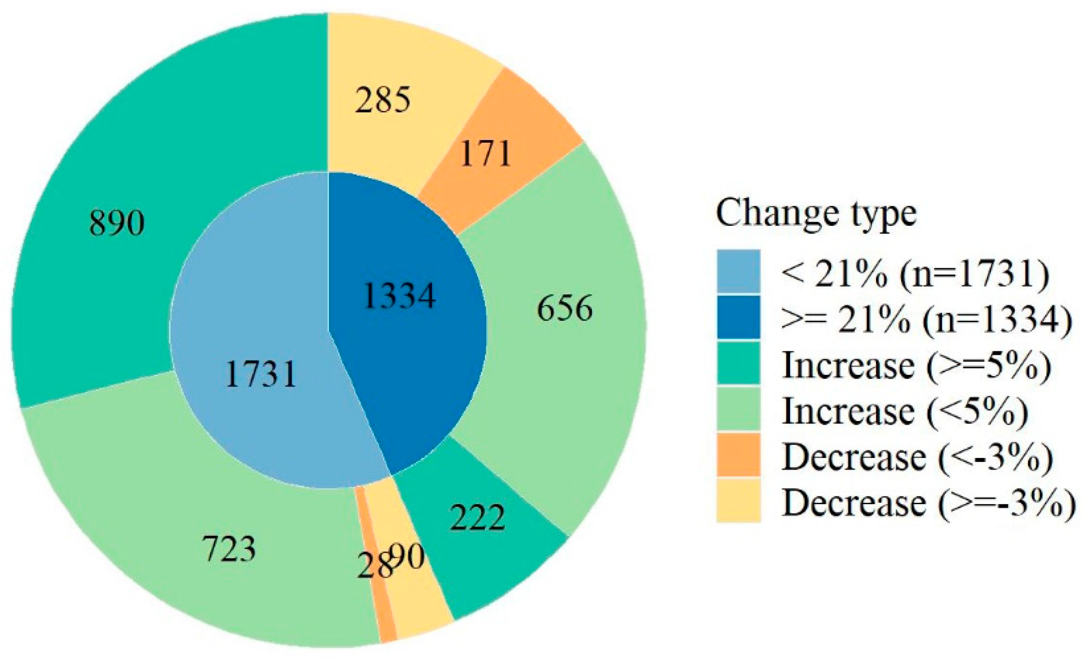
3.1. Increased Greenspace with More Fragmentation

During the period of 2005–2015, the greenspace underwent considerable changes with a net increase of 1472 ha (7.8%) (Figure 3). The total area of greenspace increased from 18,728 ha in 2005 to 20,201 ha in 2015, including 2499 ha of newly built patches, 4795 ha of expanded patches, and 5335 ha of shrinking patches (Figure 4). There were 487 ha greenspace that vanished.

Meanwhile, the greenspace experienced an increase in fragmentation with the average patch size reduced from 0.5 ha in 2005 to 0.1 ha in 2015. Results indicated an increase in small (<0.5 ha) and medium patches (0.5–4 ha), as well as a decrease in large patches (>4 ha) (Figure 5). The major net increase that occurred in small patches was 2397 ha (163% of the total net increase), compared with a net increase of 372 ha in medium patches (25% of the total net increase) and a net loss of 1296 ha in large patches (88% of the total net increase). In addition, 155 large patches broke into small/medium patches losing 608 ha, while small/medium patches merged and generated 91 large patches, increasing to 392 ha.

3.2. Improved Accessibility with Reduced Inequality

There were 3117 neighborhoods in 2005 and 3570 neighborhoods in 2015. This analysis focused on the 3065 neighborhoods existing in both 2005 and 2015 and compared their accessible greenspace, defined as percent greenspace within a 500 m buffer along the boundary of each neighborhood (referred to as “accessible greenspace” hereafter). Results indicated that accessible greenspace increased from an average of 21% in 2005 to 24% in 2015 (Figure 6). Over 80% of neighborhoods had accessible greenspace increase by an average of five percent points.

Meanwhile, the difference of accessible greenspace between neighborhoods reduced. Standard deviation of accessible greenspace reduced from 8% to 7%. This means that accessible greenspace exhibited a tendency to get closer to the mean value. Furthermore, neighborhoods with less than average accessible greenspace (<21%) had more greenspace increase compared to the rest. There were 1731 neighborhoods with accessible greenspace below the average, among which 1613 (93%) neighborhoods had their accessible greenspace increased (Figure 7). In contrast, in the remaining neighborhoods where accessible greenspace was higher than average, only 878 neighborhoods had accessible greenspace increased (66%).

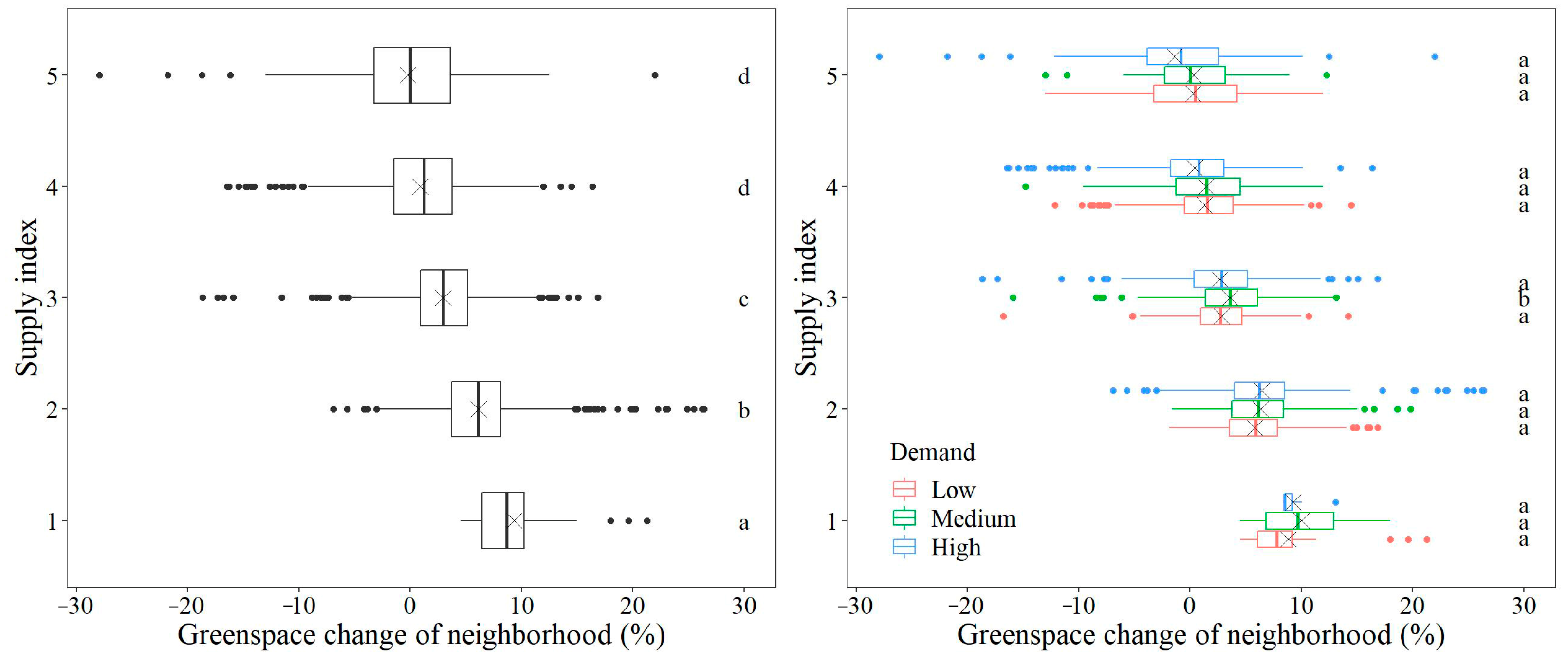
3.3. Greenspace Changes under Different Supply and Demand Levels

Results showed that greenspace increased more in neighborhoods with a lower-than-average greenspace supply in 2005 (Figure 8). We grouped neighborhoods into five categories according to their greenspace supply in 2005 (much lower than average, lower than average, average, higher than average, and much higher than average), and found that the amount of greenspace increase reduced with the increase in supply in 2005 (Figure 9a). In contrast, the change of greenspace showed little difference across different demand levels (Figure 9b). Neighborhoods with a high demand did not receive greater greenspace increase between 2005–2015.

4. Discussion

4.1. Fragmented Greenspace, Increased Accessibility

Results indicated that greenspace experienced a lot of changes during the period of 2005–2015. This finding is consistent with previous studies, concluding that even areas that are highly urbanized are often dynamic in land-cover change [50,52,81,82,83]. In addition, we found that greenspace turned out to be more fragmented, which is often considered to have a negative impact on biodiversity conservation [84,85] and the regulation of ecosystem service, such as heat mitigation [37]. However, the increased accessibility is largely benefited from the more dispersed greenspace distribution. If the primary goal of greenspace construction is to increase accessibility, especially in the densely populated urban core area, it is inevitable to have a growing number of small greenspace patches. In that case, the trend of fragmentation should not be simply interpreted as a “negative” consequence. While many studies investigated greenspace distribution [86,87] as well as its change over time [52,83], seldom did researchers measure its impact on accessibility at the same time. This study indicated that both fragmentation and accessibility increased between 2005–2015 in Beijing, which may constitute a trade-off for greenspace planning, especially in densely populated urban areas.

4.2. Where to Put New Greenspace: Supply Considered, Demand Not Considered

Greenspace change is found to be associated with existing supply. Areas with less supply tended to have a higher greenspace increase. Therefore, ten years of greening not only improved the overall greenspace accessibility, but also reduced its disparity across neighborhoods. This finding is in contrast to previous studies indicating that areas with abundant greenspace tended to get greener through tree-planting programs [51,88]. In addition to the increase in the total greenspace, improved equality in spatial distribution is a significant achievement, which delivered benefits to areas that used to lack greenspace.

With that being said, the greening efforts failed to respond to different demand levels. We found little association between greenspace change and its demand, meaning all the neighborhoods were considered to have the same demand for accessible greenspace in spite of their differences in population, age structure, or economic status of residents. Our findings indicated that demands for greenspace may vary substantially across neighborhoods, which is consistent with previous studies [89]. For example, neighborhoods with a large number of residents would need more greenspace. People of lower economic status, children, and elderly people usually rely more on greenspace within walking distance [25,53,65]. Ideally, neighborhoods with a higher proportion of these people should be prioritized with enough accessible greenspace. However, as shown in our results, the amount of greenspace change did not echo different levels of demand. In order to better meet people’s demand with limited greening resource, future urban greening projects should target areas of low supply and high demand.

It is also worth noting that in this study, we considered demand for greenspace only by amount without addressing the difference in quality. We did not consider choice or arrangement of vegetation, facilities, or maintenance, which are all important factors to deliver services to residents. This is a simplification and by no means do we suggest overlooking the qualitative side of greenspace demand. People may like native (or exotic) plants in a greenspace, be attracted by specific facilities (trail, playground, etc.), or prefer well-managed (or semi wild) greenspace. These factors were not considered in this study due to limited resources. Future work may evaluate to what extent the supply of certain greenspace qualities matches people’s preference. In order to better serve the residents, it is always essential to understand and consider their demands in urban greening projects.

4.3. Implications: Hotspot Areas for Future Greening

This study analyzed accessible greenspace change between 2005–2015 and estimated neighborhoods’ demand for greenspace. Based on the results, we can further identify areas with limited accessible greenspace but relatively high demand. For example, there were 590 neighborhoods having high demand for greenspace but less than average accessible greenspace in 2015 (<24%) (Figure 10). Among them, 422 neighborhoods’ accessible greenspace increased since 2005, whereas 168 decreased. We identified the 168 neighborhoods on a map (Figure 10). In order to meet the residents’ demand, future greening efforts should consider these 168 neighborhoods in particular. This example illustrated that combining greenspace supply, demand, and their dynamic over time through spatial analysis could help to target hotspot areas for future greening.

5. Conclusions

This study examined change of greenspace between 2005–2015 as well as the demand for greenspace by neighborhood based on the population, age structure, and economic status of residents. Our results indicated that the net increase of greenspace was 1472 ha (or 7.8%) from 2005 to 2015. Greenspace tended to be more fragmented. Neighborhoods’ accessibility to greenspace improved substantially, and the disparity between neighborhood accessible greenspace reduced. Greenspace change was associated with existing supply. Areas with relatively low supply often received greater increases in greenspace. In contrast, greenspace change was not related to its demand. To better meet people’s demand with respect to limited greenspace, we argue that future greening efforts should consider both supply and demand. We further provided an example on how to identify specific areas that need greenspace the most by overlaying neighborhoods with below-average accessible greenspace in 2015, high demand, and loss of greenspace since 2005.

Our research focused on the amount of greenspace, while greenspace quality also plays an important role in terms of meeting residents’ demand. Future studies may look into how greenspace supply and construction meet people’s preference and demand in terms of facilities, vegetation, and management. Considering demand, supply, and the changing trend of greenspace would help to allocate future greening projects, reduce disparity, and meet people’s demand.

References

1. Canedoli, C.; Bullock, C.; Collier, M.J.; Joyce, D.; Padoa-Schioppa, E. Public Participatory Mapping of Cultural Ecosystem Services: Citizen Perception and Park Management in the Parco Nord of Milan (Italy). Sustainability 2017, 9, 891. [Google Scholar] [CrossRef] [Green Version]
2. Kabisch, N.; Haase, D. Green justice or just green? Provision of urban green spaces in Berlin, Germany. Landsc. Urban Plan. 2014, 122, 129–139. [Google Scholar] [CrossRef]
3. Nowak, D.J.; Crane, D.E.; Stevens, J.C. Air pollution removal by urban trees and shrubs in the United States. Urban For. Urban Green. 2006, 4, 115–123. [Google Scholar] [CrossRef]
4. Thomas, G.; Sherin, A.P.; Ansar, S.; Zachariah, E.J. Analysis of urban heat island in Kochi, India, using a modified local climate zone classification. Procedia Environ. Sci. 2014, 21, 3–13. [Google Scholar] [CrossRef] [Green Version]
5. Yan, J.; Lin, L.; Zhou, W.; Ma, K.; Pickett, S.T.A. A novel approach for quantifying particulate matter distribution on leaf surface by combining SEM and object-based image analysis. Remote Sens. Environ. 2016, 173, 156–161. [Google Scholar] [CrossRef]
6. Xu, C.; Rahman, M.; Haase, D.; Wu, Y.; Su, M.; Pauleit, S. Surface runoff in urban areas: The role of residential cover and urban growth form. J. Clean. Prod. 2020, 262, 121421. [Google Scholar] [CrossRef]
7. Chen, W.Y. The role of urban green infrastructure in offsetting carbon emissions in 35 major Chinese cities: A nationwide estimate. Cities 2015, 44, 112–120. [Google Scholar] [CrossRef]
8. Ferenc, M.; Sedláček, O.; Fuchs, R. How to improve urban greenspace for woodland birds: Site and local-scale determinants of bird species richness. Urban Ecosyst. 2013, 17, 625–640. [Google Scholar] [CrossRef]
9. Roces-Diaz, J.V.; Vayreda, J.; Banque-Casanovas, M.; Cuso, M.; Anton, M.; Bonet, J.A.; Brotons, L.; De Caceres, M.; Herrando, S.; Martinez de Aragon, J.; et al. Assessing the distribution of forest ecosystem services in a highly populated Mediterranean region. Ecol. Indic. 2018, 93, 986–997. [Google Scholar] [CrossRef] [Green Version]
10. Andersson, E.; Barthel, S.; Borgstrom, S.; Colding, J.; Elmqvist, T.; Folke, C.; Gren, A. Reconnecting Cities to the Biosphere: Stewardship of Green Infrastructure and Urban Ecosystem Services. Ambio 2014, 43, 445–453. [Google Scholar] [CrossRef] [Green Version]
11. Dickinson, D.C.; Hobbs, R.J. Cultural ecosystem services: Characteristics, challenges and lessons for urban green space research. Ecosyst. Serv. 2017, 25, 179–194. [Google Scholar] [CrossRef]
12. Wolch, J.R.; Byrne, J.; Newell, J.P. Urban green space, public health, and environmental justice: The challenge of making cities ‘just green enough’. Landsc. Urban Plan. 2014, 125, 234–244. [Google Scholar] [CrossRef] [Green Version]
13. Sugiyama, T.; Leslie, E.; Giles-Corti, B.; Owen, N. Associations of neighbourhood greenness with physical and mental health: Do walking, social coherence and local social interaction explain the relationships? J. Epidemiol. Commun. Health 2008, 62, e9. [Google Scholar] [CrossRef] [PubMed] [Green Version]
14. MilliontreeNYC. Million Trees NYC. 2007. Available online: https://www.milliontreesnyc.org (accessed on 25 June 2021).
15. Beijing Gerdening and Greening Bureau. One Million Acres Plain Afforestation Project. Available online: http://yllhj.beijing.gov.cn/ztxx/mtjj/mtbd/201602/t20160206_115734.shtml (accessed on 25 June 2021).
16. Shih, W.Y.; Ahmad, S.; Chen, Y.C.; Lin, T.P.; Mabon, L. Spatial relationship between land development pattern and intra-urban thermal variations in Taipei. Sustain. Cities Soc. 2020, 62, 102415. [Google Scholar] [CrossRef]
17. Zhang, Y.; Murray, A.T.; Turner, B.L. Optimizing green space locations to reduce daytime and nighttime urban heat island effects in Phoenix, Arizona. Landsc. Urban Plan. 2017, 165, 162–171. [Google Scholar] [CrossRef]
18. Evenson, K.R.; Wen, F.; Hillier, A.; Cohen, D.A. Assessing the contribution of parks to physical activity using global positioning system and accelerometry. Med. Sci. Sports Exerc. 2013, 45, 1981–1987. [Google Scholar] [CrossRef] [Green Version]
19. Song, P.H.; Kim, G.; Mayer, A.; He, R.Z.; Tian, G.H. Assessing the Ecosystem Services of Various Types of Urban Green Spaces Based on i-Tree Eco. Sustainability 2020, 12, 1630. [Google Scholar] [CrossRef] [Green Version]
20. Zhang, S.; Zhou, W. Recreational visits to urban parks and factors affecting park visits: Evidence from geotagged social media data. Landsc. Urban Plan. 2018, 180, 27–35. [Google Scholar] [CrossRef]
21. Li, L.J.; Du, Q.Y.; Ren, F.; Ma, X.Y. Assessing Spatial Accessibility to Hierarchical Urban Parks by Multi-Types of Travel Distance in Shenzhen, China. Int. J. Environ. Res. Public Health 2019, 16, 1038. [Google Scholar] [CrossRef] [Green Version]
22. Tan, C.D.; Tang, Y.H.; Wu, X.F. Evaluation of the Equity of Urban Park Green Space Based on Population Data Spatialization: A Case Study of a Central Area of Wuhan, China. Sensors 2019, 19, 2929. [Google Scholar] [CrossRef] [Green Version]
23. Xing, L.; Liu, Y.; Liu, X. Measuring spatial disparity in accessibility with a multi-mode method based on park green spaces classification in Wuhan, China. Appl. Geogr. 2018, 94, 251–261. [Google Scholar] [CrossRef]
24. Xu, C.; Haase, D.; Pribadi, D.O.; Pauleit, S. Spatial variation of green space equity and its relation with urban dynamics: A case study in the region of Munich. Ecol. Indic. 2018, 93, 512–523. [Google Scholar] [CrossRef]
25. Chen, B.; Qi, X.; Qiu, Z. Recreational use of urban forest parks: A case study in Fuzhou National Forest Park, China. J. For. Res. 2018, 23, 183–189. [Google Scholar] [CrossRef]
26. Huang, J.H.; Hipp, J.A.; Marquet, O.; Alberico, C.; Fry, D.; Mazak, E.; Lovasi, G.S.; Robinson, W.R.; Floyd, M.F. Neighborhood characteristics associated with park use and park-based physical activity among children in low-income diverse neighborhoods in New York City. Prev. Med. 2020, 131, 105948. [Google Scholar] [CrossRef] [PubMed]
27. Wang, D.; Brown, G.; Zhong, G.; Liu, Y.; Mateo-Babiano, I. Factors influencing perceived access to urban parks: A comparative study of Brisbane (Australia) and Zhongshan (China). Habitat. Int. 2015, 50, 335–346. [Google Scholar] [CrossRef]
28. Kukulska-Kozieł, A.; Szylar, M.; Cegielska, K.; Noszczyk, T.; Gawroński, K.; Dixon-Gough, R.; Jombach, S.; Valánszki, I.; Kovács, K.F. Towards three decades of spatial development transformation in two contrasting post-Soviet cities—Kraków and Budapest. Land Use Policy 2019, 85, 328–339. [Google Scholar] [CrossRef]
29. Puplampu, D.A.; Boafo, Y.A. Exploring the impacts of urban expansion on green spaces availability and delivery of ecosystem services in the Accra metropolis. Environ. Chall. 2021, 5, 100283. [Google Scholar] [CrossRef]
30. Fernández-Juricic, E.; Jokimäki, J. A habitat island approach to conserving birds in urban landscapes: Case studies from southern and northern Europe. Biodivers. Conserv. 2001, 10, 2023–2043. [Google Scholar] [CrossRef]
31. Xie, S.; Lu, F.; Cao, L.; Zhou, W.; Ouyang, Z. Multi-scale factors influencing the characteristics of avian communities in urban parks across Beijing during the breeding season. Sci. Rep. 2016, 6, 29350. [Google Scholar] [CrossRef]
32. Turo, K.J.; Spring, M.R.; Sivakoff, F.S.; Delgado de la flor, Y.A.; Gardiner, M.M.; Garibaldi, L. Conservation in post-industrial cities: How does vacant land management and landscape configuration influence urban bees? J. Appl. Ecol. 2020, 58, 58–69. [Google Scholar] [CrossRef]
33. Xie, S.; Wang, X.; Zhou, W.; Wu, T.; Qian, Y.; Lu, F.; Gong, C.; Zhao, H.; Ouyang, Z. The effects of residential greenspace on avian Biodiversity in Beijing. Glob. Ecol. Conserv. 2020, 24, e01223. [Google Scholar] [CrossRef]
34. Li, X.; Zhou, W. Optimizing urban greenspace spatial pattern to mitigate urban heat island effects: Extending understanding from local to the city scale. Urban For. Urban Green. 2019, 41, 255–263. [Google Scholar] [CrossRef]
35. Li, X.; Zhou, W.; Ouyang, Z. Relationship between land surface temperature and spatial pattern of greenspace: What are the effects of spatial resolution? Landsc. Urban Plan. 2013, 114, 1–8. [Google Scholar] [CrossRef]
36. Qian, Y.; Zhou, W.; Hu, X.; Fu, F. The Heterogeneity of Air Temperature in Urban Residential Neighborhoods and Its Relationship with the Surrounding Greenspace. Remote Sens. 2018, 10, 965. [Google Scholar] [CrossRef] [Green Version]
37. Zhou, W.; Wang, J.; Cadenasso, M.L. Effects of the spatial configuration of trees on urban heat mitigation: A comparative study. Remote Sens. Environ. 2017, 195, 1–12. [Google Scholar] [CrossRef]
38. Zandieh, R.; Martinez, J.; Flacke, J. Older Adults’ Outdoor Walking and Inequalities in Neighbourhood Green Spaces Characteristics. Int. J. Environ. Res. Public Health 2019, 16, 4379. [Google Scholar] [CrossRef] [Green Version]
39. Dai, D. Racial/ethnic and socioeconomic disparities in urban green space accessibility: Where to intervene? Landsc. Urban Plan. 2011, 102, 234–244. [Google Scholar] [CrossRef]
40. Macedo, J.; Haddad, M.A. Equitable distribution of open space: Using spatial analysis to evaluate urban parks in Curitiba, Brazil. Environ. Plan. B Plan. Des. 2016, 43, 1096–1117. [Google Scholar] [CrossRef]
41. Nesbitt, L.; Meitner, M.J.; Girling, C.; Sheppard, S.R.J.; Lu, Y. Who has access to urban vegetation? A spatial analysis of distributional green equity in 10 US cities. Landsc. Urban Plan. 2019, 181, 51–79. [Google Scholar] [CrossRef]
42. Lin, B.B.; Fuller, R.A.; Bush, R.; Gaston, K.J.; Shanahan, D.F. Opportunity or orientation? Who uses urban parks and why. PLoS ONE 2014, 9, e87422. [Google Scholar] [CrossRef] [Green Version]
43. Zhou, W.; Huang, G.; Pickett, S.T.A.; Cadenasso, M.L. 90 years of forest cover change in an urbanizing watershed: Spatial and temporal dynamics. Landsc. Ecol. 2011, 26, 645–659. [Google Scholar] [CrossRef]
44. Baro, F.; Calderon-Argelich, A.; Langemeyer, J.; Connolly, J.J.T. Under one canopy? Assessing the distributional environmental justice implications of street tree benefits in Barcelona. Environ. Sci. Policy 2019, 102, 54–64. [Google Scholar] [CrossRef]
45. Boone, C.G.; Buckley, G.L.; Grove, J.M.; Sister, C. Parks and People: An Environmental Justice Inquiry in Baltimore, Maryland. Ann. Assoc. Am. Geogr. 2009, 99, 767–787. [Google Scholar] [CrossRef]
46. Lara-Valencia, F.; Garcia-Perez, H. Disparities in the provision of public parks in neighbourhoods with varied Latino composition in the Phoenix Metropolitan Area. Local Environ. 2018, 23, 1107–1120. [Google Scholar] [CrossRef]
47. You, H. Characterizing the inequalities in urban public green space provision in Shenzhen, China. Habitat. Int. 2016, 56, 176–180. [Google Scholar] [CrossRef]
48. Guo, T.D.; Morgenroth, J.; Conway, T.; Xu, C. City-wide canopy cover decline due to residential property redevelopment in Christchurch, New Zealand. Sci. Total Environ. 2019, 681, 202–210. [Google Scholar] [CrossRef]
49. Qian, Y.G.; Li, Z.Q.; Zhou, W.Q.; Chen, Y.Y. Quantifying spatial pattern of urban greenspace from a gradient perspective of built-up age. Phys. Chem. Earth 2019, 111, 78–85. [Google Scholar] [CrossRef]
50. Wang, J.; Zhou, W.; Qian, Y.; Li, W.; Han, L. Quantifying and characterizing the dynamics of urban greenspace at the patch level: A new approach using object-based image analysis. Remote Sens. Environ. 2018, 204, 94–108. [Google Scholar] [CrossRef]
51. Casey, J.A.; James, P.; Cushing, L.; Jesdale, B.M.; Morello-Frosch, R. Race, Ethnicity, Income Concentration and 10-Year Change in Urban Greenness in the United States. Int. J. Environ. Res. Public Health 2017, 14, 1546. [Google Scholar] [CrossRef] [PubMed] [Green Version]
52. Timilsina, S.; Aryal, J.; Kirkpatrick, J.B. Mapping Urban Tree Cover Changes Using Object-Based Convolution Neural Network (OB-CNN). Remote Sens. 2020, 12, 3017. [Google Scholar] [CrossRef]
53. Liu, H.; Li, F.; Xu, L.; Han, B. The impact of socio-demographic, environmental, and individual factors on urban park visitation in Beijing, China. J. Clean. Prod. 2017, 163, S181–S188. [Google Scholar] [CrossRef]
54. Yen, Y.; Wang, Z.; Shi, Y.; Xu, F.; Soeung, B.; Sohail, M.T.; Rubakula, G.; Juma, S.A. The predictors of the behavioral intention to the use of urban green spaces: The perspectives of young residents in Phnom Penh, Cambodia. Habitat. Int. 2017, 64, 98–108. [Google Scholar] [CrossRef]
55. Mertens, L.; Van Cauwenberg, J.; Veitch, J.; Deforche, B.; Van Dyck, D. Differences in park characteristic preferences for visitation and physical activity among adolescents: A latent class analysis. PLoS ONE 2019, 14, e0212920. [Google Scholar] [CrossRef] [PubMed]
56. Contesse, M.; van Vliet, B.J.M.; Lenhart, J. Is urban agriculture urban green space? A comparison of policy arrangements for urban green space and urban agriculture in Santiago de Chile. Land Use Policy 2018, 71, 566–577. [Google Scholar] [CrossRef]
57. Martinho da Silva, I.; Oliveira Fernandes, C.; Castiglione, B.; Costa, L. Characteristics and motivations of potential users of urban allotment gardens: The case of Vila Nova de Gaia municipal network of urban allotment gardens. Urban For. Urban Green. 2016, 20, 56–64. [Google Scholar] [CrossRef]
58. Zinia, N.J.; McShane, P. Ecosystem services management: An evaluation of green adaptations for urban development in Dhaka, Bangladesh. Landsc. Urban Plan. 2018, 173, 23–32. [Google Scholar] [CrossRef]
59. Andrews, B.; Ferrini, S.; Bateman, I. Good parks—Bad parks: The influence of perceptions of location on WTP and preference motives for urban parks. J. Environ. Econ. Manag. 2017, 6, 204–224. [Google Scholar] [CrossRef]
60. Latinopoulos, D.; Mallios, Z.; Latinopoulos, P. Valuing the benefits of an urban park project: A contingent valuation study in Thessaloniki, Greece. Land Use Policy 2016, 55, 130–141. [Google Scholar] [CrossRef]
61. Gu, X.K.; Li, Q.; Chand, S. Factors influencing residents’ access to and use of country parks in Shanghai, China. Cities 2020, 97, 102501. [Google Scholar] [CrossRef]
62. Shan, X.Z. Association between the time patterns of urban green space visitations and visitor characteristics in a high-density, subtropical city. Cities 2020, 97, 102562. [Google Scholar] [CrossRef]
63. Sun, R.H.; Li, F.; Chen, L.D. A demand index for recreational ecosystem services associated with urban parks in Beijing, China. J. Environ. Manag. 2019, 251. [Google Scholar] [CrossRef]
64. Ghahramani, M.; Galle, N.J.; Duarte, F.; Ratti, C.; Pilla, F. Leveraging artificial intelligence to analyze citizens’ opinions on urban green space. City Environ. Interact. 2021, 10, 100058. [Google Scholar] [CrossRef]
65. Xing, L.; Liu, Y.; Liu, X.; Wei, X.; Mao, Y. Spatio-temporal disparity between demand and supply of park green space service in urban area of Wuhan from 2000 to 2014. Habitat. Int. 2018, 71, 49–59. [Google Scholar] [CrossRef]
66. Beijing Municipal Bureau Statistics (BMBS). The Changes and Characteristics of Beijing’s Population Development in 2014. Available online: http://tjj.beijing.gov.cn/zxfbu/202002/t20200216_1636952.html (accessed on 25 June 2021).
67. Qian, Y.; Zhou, W.; Li, W.; Han, L. Understanding the dynamic of greenspace in the urbanized area of Beijing based on high resolution satellite images. Urban For. Urban Green. 2015, 14, 39–47. [Google Scholar] [CrossRef]
68. Qian, Y.; Zhou, W.; Yu, W.; Pickett, S.T.A. Quantifying spatiotemporal pattern of urban greenspace: New insights from high resolution data. Landsc. Ecol. 2015, 30, 1165–1173. [Google Scholar] [CrossRef]
69. Yan, J.; Zhou, W.; Zheng, Z.; Wang, J.; Tian, Y. Characterizing variations of greenspace landscapes in relation to neighborhood characteristics in urban residential area of Beijing, China. Landsc. Ecol. 2019, 35, 203–222. [Google Scholar] [CrossRef]
70. Gaode Map. The Boundary of Neighborhoods. 2018. Available online: https://ditu.amap.com (accessed on 25 June 2021).
71. Lianjia Web. The House Price and Age of Neighborhoods. 2018. Available online: http://bj.lianjia.com (accessed on 25 June 2021).
72. Tu, X. Impact of Urban Park Characteristics and Spatial Patterns Recreational Services to Residents: The Case Study of Beijing. Ph.D. Thesis, Beijing Normal University, Beijing, China, 1 December 2019. [Google Scholar]
73. Beijing Municipal Bureau Statistics (BMBS). Beijing Statistical Yearbook in 2006. Available online: http://tjj.beijing.gov.cn (accessed on 25 June 2021).
74. Rogan, J.; Chen, D. Remote sensing technology for mapping and monitoring land-cover and land-use change. Prog. Plan. 2004, 61, 301–325. [Google Scholar] [CrossRef]
75. Stow, D.A. Reducing the effects of misregistration on pixel-level change detection. Int. J. Remote Sens. 1999, 20, 2477–2483. [Google Scholar] [CrossRef]
76. Zhou, J.; Yu, B.; Qin, J. Multi-Level Spatial Analysis for Change Detection of Urban Vegetation at Individual Tree Scale. Remote Sens. 2014, 6, 9086–9103. [Google Scholar] [CrossRef] [Green Version]
77. Peschardt, K.K.; Schipperijn, J.; Stigsdotter, U.K. Use of Small Public Urban Green Spaces (SPUGS). Urban For. Urban Green. 2012, 11, 235–244. [Google Scholar] [CrossRef]
78. Wilkerson, M.L.; Mitchell, M.G.E.; Shanahan, D.; Wilson, K.A.; Ives, C.D.; Lovelock, C.E.; Rhodes, J.R. The role of socio-economic factors in planning and managing urban ecosystem services. Ecosyst. Serv. 2018, 31, 102–110. [Google Scholar] [CrossRef]
79. Boone, C.G. Improving resolution of census data in metropolitan areas using a dasymetric approach: Applications for the Baltimore Ecosystem Study. Cities Environ. 2008, 1, 3. [Google Scholar] [CrossRef]
80. Tu, X.; Huang, G.; Wu, J. Contrary to Common Observations in the West, Urban Park Access Is Only Weakly Related to Neighborhood Socioeconomic Conditions in Beijing, China. Sustainability 2018, 10, 1115. [Google Scholar] [CrossRef] [Green Version]
81. Cui, L.; Wang, J.; Sun, L.; Lv, C. Construction and optimization of green space ecological networks in urban fringe areas: A case study with the urban fringe area of Tongzhou district in Beijing. J. Clean. Prod. 2020, 276, 124266. [Google Scholar] [CrossRef]
82. Zhou, W.; Wang, J.; Qian, Y.; Pickett, S.T.A.; Li, W.; Han, L. The rapid but “invisible” changes in urban greenspace: A comparative study of nine Chinese cities. Sci. Total Environ. 2018, 627, 1572–1584. [Google Scholar] [CrossRef] [PubMed]
83. Song, Y.; Aryal, J.; Tan, L.; Jin, L.; Gao, Z.; Wang, Y. Comparison of changes in vegetation and land cover types between Shenzhen and Bangkok. Land Degrad Dev. 2020, 32, 1192–1204. [Google Scholar] [CrossRef]
84. Cheng, X.L.; Nizamani, M.M.; Jim, C.Y.; Balfour, K.; Da, L.J.; Qureshi, S.; Zhu, Z.X.; Wang, H.-F. Using SPOT Data and FRAGSTAS to Analyze the Relationship between Plant Diversity and Green Space Landscape Patterns in the Tropical Coastal City of Zhanjiang, China. Remote Sens. 2020, 12, 3477. [Google Scholar] [CrossRef]
85. Plummer, K.E.; Gillings, S.; Siriwardena, G.M.; Villard, M.A. Evaluating the potential for bird-habitat models to support biodiversity-friendly urban planning. J. Appl. Ecol. 2020, 57, 1902–1914. [Google Scholar] [CrossRef]
86. Shekhar, S.; Aryal, J. Role of geospatial technology in understanding urban green space of Kalaburagi city for sustainable planning. Urban For. Urban Green. 2019, 46, 126450. [Google Scholar] [CrossRef]
87. Mathieu, R.; Aryal, J.; Chong, A.K. Object-based classification of IKONOS imagery for mapping. Sensors 2007, 7, 2860–2880. [Google Scholar] [CrossRef] [Green Version]
88. Garrison, J.D. Seeing the park for the trees: New York’s ‘‘Million Trees’’ campaign vs. the deep roots of environmental inequality. Environ. Plan. B Urban Anal. City Sci. 2019, 46, 914–930. [Google Scholar] [CrossRef]
89. Zhang, Y.; Zhang, T.; Zeng, Y.; Yu, C.; Zheng, S. The rising and heterogeneous demand for urban green space by Chinese urban residents: Evidence from Beijing. J. Clean. Prod. 2021, 313, 127781. [Google Scholar] [CrossRef]
Figure 1. Study area: Neighborhoods within fifth ring road in Beijing, China.
Remotesensing 13 04310 g001
Figure 2. Schematic diagram of false-change recognition. (a) The identified “changed part” was small and shared some boundaries with the original patch; (b) the identified “changed part” was relatively large but no larger than the original patch. It shared more than a quarter of its boundary with the original patch. In the equations, C   is the changed part; S is the original patch; A C is the area of the changed part; A S is the area of original patch; C   S is the length of boundary shared by C and S; T is a fraction indicating size threshold relative to AS; and P c is the perimeter of C.
Remotesensing 13 04310 g002
Figure 3. Greenspace in 2005 and 2015, and its change. (a) Greenspace in 2005; (b) Greenspace in 2015; (c) Greenspace change from 2005–2015.
Remotesensing 13 04310 g003
Figure 4. Area of greenspace change from 2005 to 2015. Decrease in greenspace included vanished and shrinking patches. Increase in greenspace included new patches and existing patches that have been expanded.
Remotesensing 13 04310 g004
Figure 5. Change in differently sized greenspace patches from 2005 to 2015.
Remotesensing 13 04310 g005
Figure 6. Accessible greenspace and its change in the 3065 neighborhoods. We define accessible greenspace as the percentage of greenspace within a 500 m buffer along the boundary of each neighborhood. The two boxplots on the left represent accessible greenspace in 2005 and 2015 with average values of 21% and 24%, respectively. The two boxplots on the right represent the change in accessible greenspace from 2005 to 2015, which decreased in 574 neighborhoods by 3% and increased in 2491 neighborhoods by 5%.
Remotesensing 13 04310 g006
Figure 7. Difference in greenspace change during the period of 2005–2015 between neighborhoods with a higher than average greenspace accessibility in 2005 (21%) and all other neighborhoods.
Remotesensing 13 04310 g007
Figure 8. Greenspace supply and demand by neighborhood. (a) Accessible greenspace of neighborhood in 2005 (%); (b) Accessible greenspace of neighborhood in 2015 (%); (c) Accessible greenspace change of neighborhood from 2005–2015; (d) Demand level of greenspace by neighborhood.
Remotesensing 13 04310 g008
Figure 9. Association between greenspace increase with (a) greenspace supply in 2005 and (b) different levels of demand (high, medium, and low).
Remotesensing 13 04310 g009
Figure 10. Greenspace change in neighborhoods with less than average accessible greenspace (24%) and high demand.
Remotesensing 13 04310 g010