Sentinel-2 Time Series Analysis for Identification of Underutilized Land in Europe

Abstract

Biomass and bioenergy play a central role in Europe’s Green Transition. Currently, biomass is representing half of the renewable energy sources used. While the role of renewables in the energy mix is undisputed, there have been many controversial discussions on the use of biomass for energy due to the “food versus fuel” debate. Using previously underutilized lands for bioenergy is one possibility to prevent this discussion. This study supports the attempts to increase biomass for bioenergy through the provision of improved methods to identify underutilized lands in Europe. We employ advanced analysis methods based on time series modelling using Sentinel-2 (S2) data from 2017 to 2019 in order to distinguish utilized from underutilized land in twelve study areas in different bio-geographical regions (BGR) across Europe. The calculated parameters of the computed model function combined with temporal statistics were used to train a random forest classifier (RF). The achieved overall accuracies (OA) per study area vary between 80.25 and 96.76%, with confidence intervals (CI) ranging between 1.77% and 6.28% at a 95% confidence level. All in all, nearly 500,000 ha of underutilized land potentially available for agricultural bioenergy production were identified in this study, with the greatest amount mapped in Eastern Europe.

1. Introduction

Biomass as a source of renewable energy production plays an essential role in Europe’s Green Transition [1]. The European Union’s (EU) Revised Renewable Energy Directive requests 32% of EU’s energy production to originate from renewables. Moreover, bioenergy represents a valuable option to support the implementation of the Sustainable Development Goals (SDGs) of the United Nations (UN), especially SDG Nr. 7: “Ensure access to affordable, reliable, sustainable and modern energy for all” and Nr. 13: “Take urgent action to combat climate change and its impacts” [2]. The IPCC special report on the impacts of global warming 1.5° also highlights the importance of bioenergy “due to its multiple roles in decarbonizing energy” [3]. The IPCC report and the EU explicitly state that bioenergy should be produced in a sustainable manner at all levels along the entire value chain and must not affect agricultural or food systems, biodiversity and various other ecosystem functions and services [3,4]. One approach to prevent the food vs. fuel competition is the use of contaminated, underutilized and/or marginal land that cannot be used for food or feed production but still retains the potential to produce biomass feedstock for bioenergy purposes [2,5,6]. Several studies concluded that using these lands for bioenergy production could have positive environmental and socio-economic impacts [7,8,9,10].

Generally, a land is considered to be underutilized when there is no sign of any human intervention over a certain period. The Food and Agriculture Organization (FAO) of the United Nations (UN) [11], for example, uses an idle period of five years in its definition. In this study, we used a period of three years due to the availability of S2 data from 2017 onwards. With the availability of satellite image time series of high temporal resolution, remote sensing offers the possibility to generate area-wide information on land use and therefore the presence and absence of human interventions. The opening of the entire Landsat data archive and the publicly accessible data of the S2 and Moderate Resolution Imaging Spectroradiometer (MODIS) missions with global coverage, especially, increased the use of dense satellite image time series for land use monitoring purposes [12]. Various studies used MODIS data for large-area assessments of underutilized or abandoned (farm) land in Europe and Asia due to their high temporal resolution [13,14,15,16,17]. Within Europe, the former communist countries in the Eastern part of the continent have been the regions of interest in these studies, since large agricultural areas were left fallow following the collapse of the Soviet Union [13,18]. However, the main drawback of MODIS data lies in the spatial resolution of 500 m, which prevents accurate and detailed regional and local assessments in areas of small structured agriculture, typical of large parts of Europe. To bridge the gap between continental assessment and high-resolution mapping requirements [19], Landsat 8 (L8) image time series from 2015–2019 with a spatial resolution of 30 m and a temporal resolution of 16 days are used to generate a European-wide map of underutilized land. The authors employed temporal features for random forest classification using Google Earth Engine (GEE) [20]. Due to the pan-European extent, only temporal features like minimum, maximum, standard deviation, etc., are used in this approach [19]. At the regional level, Landsat time series data from 1986 until 2008 have been used [21] to map post-socialism farmland abandonment in western Ukraine.

Being part of the EU’s Copernicus program since 2017, the S2 satellites provide both higher spatial (10 m) and higher temporal (5 days) resolution optical data compared to Landsat. The potential of Sentinel-2 data for mapping and monitoring land abandonment has already been tested in several, mostly local studies, e.g., in Lithuania to map abandoned farmland [22]. Similarly, [23] used all 10 m resolution S2 bands and four derived vegetation indices of three observations to map farmland abandonment in western Slovakia. The performance of S2 to map abandoned citrus plantations on a local level in Valencia (Spain) was done [24] by employing mono-temporal S2 data in combination with airborne images from 2019 with a very high resolution (VHR). On the regional level, [25] employed S2 time series data from 2017–2020 to detect abandoned agricultural land in Valencia, including five spectral indices to evaluate the performance of different machine learning and deep learning classifiers [25].

Previous studies have shown that underutilized land (UU) has a different spectral reflectance behavior over time compared to utilized land (U) due to missing human interventions [14,19,25]. Typical human interventions are mowing and ploughing, which result in clear changes in the spectral reflectance of the respective patch of land. It was shown, that UU land usually shows different magnitudes and standard deviations of changes over time compared to utilized land due to the missing above-mentioned interventions [14,25]. Sometimes, however, temporal statistical features (TSFs) like minimum, maximum or standard deviation can be similar for different land use classes, while the temporal curve, which can be represented by time series model features (TSMFs), is very different (see Figure 1).

The aim of this study is thus to derive alternative features based on a time series model fitting of S2 imagery that captures the differences in spectral behavior of different land use classes over the course of time, other than temporal statistics. The calculated model function reconstructing the continuous spectral curve is described by a set of parameters, which depend on the employed mathematical model. Examples of these model parameters are the amplitude of the sinus or cosine, model variance or observation variance. Instead of using the modeled images (i.e., synthetic images), we analyze the performance of the model parameters to serve as classification input features to train a random forest classifier.

Therefore, the research questions to be analyzed in this study are:

• Which S2 time series model features of which spectral bands work best for the differentiation between utilized and underutilized land?
• What is the level of accuracy that can be achieved in different bio-geographical regions of Europe using a common classification approach?

2. Materials and Methods

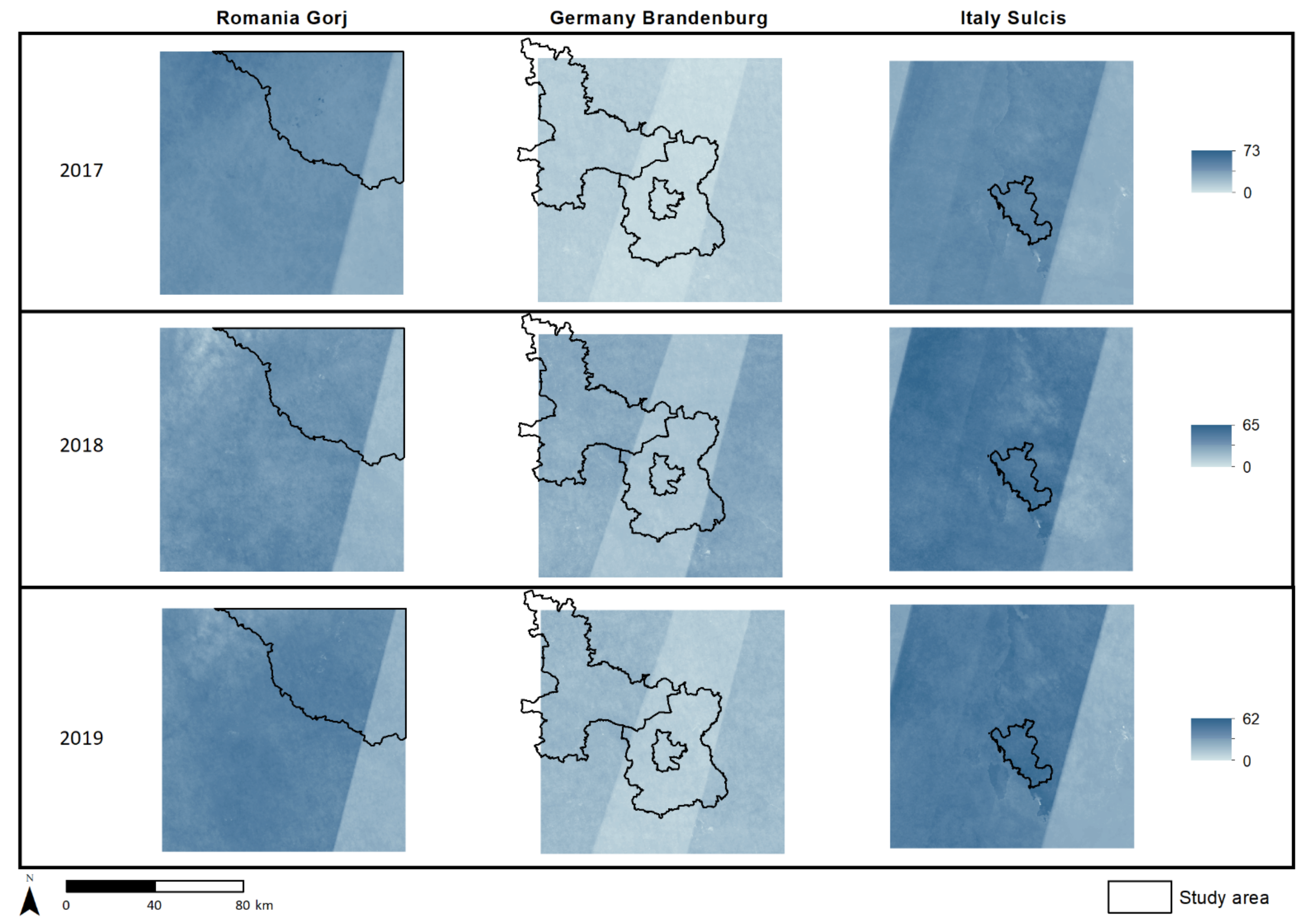
2.1. Study Area

The selection of the study areas was done by the project consortium of BIOPLAT-EU (https://bioplat.eu accessed date 8 November 2021) based on statistical data and previous knowledge of underutilized lands in these areas. The twelve study areas (see Figure 2) are spread over three biogeographical regions (BGR) and thus cover much of the variability of the appearance of underutilized lands, due to unequal environmental conditions (e.g., climate, soil etc.), to be expected within Europe, except for Scandinavia and the British and Irish islands.

Table 1. Study area properties.

No.	Study Area	Country	Biogeographical Region	Main Reason for Selection
1	Dahme Spreewald	Germany	Continental	Post-sewage farms, post-mining areas
2	Spree-Neiße
3	Bacau	Romania	Continental	Economically and topographically marginal land
4	Gorj			Post-mining areas
5	Chernihiv	Ukraine	Continental	Post-socialist fallow land
6	Khmelnytskyi
7	Bacs-Kiskun & Csongrad	Hungary	Pannonian	Economically and climatically marginal land
8	Hungary-North
9	Val Basento	Italy	Mediterranean	Areas not used due to contamination
10	Sulcis
11	Albacete	Spain	Mediterranean	Climatically marginal (dry) areas
12	Cuenca

covers the main parameters of the study areas. Since the two study areas in Germany as well as in Spain are adjacent, they are treated as one single study area in the assessment, and no separate results will be reported. More detailed information on the selection of study areas can be found here [26].

2.2. Data

2.2.1. Satellite Imagery

The Copernicus S2 mission provides high-resolution dense optical time series data for the development of Earth-Observation-based environmental monitoring systems [27]. The high temporal resolution of 5 days is obtained by having two satellites operating in the orbit carrying identical sensor systems. The whole S2 system has been fully operational since mid-2017, delivering imagery with 13 spectral bands [28]. In this study, S2 data including all 10 m and 20 m spectral bands (see

Table 2. S2 bands used in this study.

Band	Central Wavelength (nm)	Spatial Resolution (m)
B2	490 (blue)	10
B3	560 (green)	10
B4	665 (red)	10
B5	705 (red-edge)	20
B6	740 (red-edge)	20
B7	783 (red-edge)	20
B8	842 (near infrared)	10
B8A	865 (near infrared)	20
B11	1610 (short waved infrared)	20
B12	2190 (short waved infrared)	20

) from 2017–2019 were used to derive the time series features used for the classification.

2.2.2. Training Data

The visual interpretation of Google Earth VHR image time series was the main source for the compilation of a reference dataset for underutilized lands. Though being a static product, the ”Land Use/Cover Area frame statistical Survey” (LUCAS) database proved to be of valuable assistance for the identification of underutilized lands. LUCAS is a harmonized in situ (terrestrial) LCLU data collection procedure [29]. Its classification key includes two LU classes that can serve as indicators for underutilized lands (U410 “Abandoned Areas” and U420 “Semi-Natural and Natural Areas not in Use”). Details and the datasets can be obtained from the Eurostat Website [30]. LUCAS is conducted every three years, with the most recent survey having taken place in 2018. All U410 and U420 points in the study areas were visually checked and converted into polygon information, if the areas proved to be underutilized for the past three years according to data available in Google Earth. Additional reference data for underutilized lands were also gathered for the study areas in Germany, Hungary, Romania and Ukraine from local stakeholders.

A training dataset that covers all types of used land, in particular forests, settlements, annual and permanent cropland and managed grassland, was generated using a random point sampling approach with the following European-wide COPERNICUS Land Monitoring Service Products:

• High-Resolution Layers (HRL) Forest, Imperviousness and Water & Wetness
• CORINE Land Cover (CLC) 2018 agriculture classes “Arable land” (21), “Permanent crops” (22) and “Pastures” (23).

Due to their wall-to-wall structure and large amounts, no further visual interpretation was needed for these training datasets. Since the above-mentioned datasets do not cover the state of Ukraine, we used a separate land use classification provided by [31]. For the classification, all training data for different types of used land were summarized in one single class, e.g., the same label was assigned to all of them.

2.2.3. Reference Data for Exclusion of Specific Areas

As laid out in the introduction, the production of biomass for bioenergy purposes should not affect any existing agricultural or food systems or jeopardize nature’s biodiversity and various other ecosystem functions and services. Therefore, areas known to feature these functions are removed from the results. This step can be seen as a “safeguarding” procedure to ensure that, ideally, no areas used for food production are assigned to underutilized land. Due to the project’s ambition to generate close-to-practice results, we had to include this step, removing known areas used for food or feed production, steep slopes not suitable for bioenergy production and protected areas for example. All details on the exclusion of specific areas can be found in [19], where the same procedure was applied.

For the assessment, only those parts within the selected study areas that are not covered by these existing dataset are considered in the assessment and are referred as “area of interest” (AOI) in the further course of this paper (see

Table 3. Study areas and respective “areas of interest”.

No.	Study Area	Country	Study Area [ha]	Elimination Mask [ha]	Area of Interest [ha]
1	Dahme-Spreewald	Germany	394,462	307,399	87,063 s
2	Spree-Neiße
3	Bacau	Romania	530,235	407,225	123,010
4	Gorj		1,043,536	675,641	367,895
5	Chernihiv	Ukraine	581,309	230,082	351,227
6	Khmelnytskyi		1,254,216	400,755	853,461
7	Bacs-Kiskun & Csongrad	Hungary	1,192,070	606,547	585,523
8	Hungary-North		1,219,271	639,779	579,492
9	Val Basento	Italy	1,218,812	841,742	377,070
10	Sulcis		35,802	16,694	17,485
11	Albacete	Spain	2,304,810	1,285,882	1,018,928
12	Cuenca

).

2.2.4. Reference Data for Validation

To report accuracies of the mapping results, validation data were derived based on a stratified sampling approach. Based on an independent classification of underutilized lands (the map produced by [19]), we sampled the same number of points per class, e.g., utilized and underutilized land, randomly. These points were then visually interpreted using Google Earth VHR time series data using the same procedure described by [19] with two adaptations: first, the minimum mapping unit (MMU) was changed to 0.5 ha to be in line with the product definition, and second, the reference period was adapted to 2017–2019 instead of 2015–2019, since satellite image time series data from this period were employed. The weights for each class were calculated using the ratio of the area of the respective class from the independent classification [19] and the number of interpreted points. Using such an approach, the resulting accuracy measures are unbiased. Compared to the study of [19], it has been necessary to adapt two parameters for the visual interpretation of the validation points: first, the minimum mapping unit (MMU) was changed to 0.5 ha, and second, the reference period was adapted to 2017–2019 instead of 2015–2019, since satellite image time series data from this period were employed. The final number of available validation points per study area is given in

Table 4. Number of validation points per study area.

Study Area	Utilized Land	Underutilized Land	Total
Dahme-Spreewald & Spree-Neiße	173	22	195
Bacau	166	105	271
Gorj	193	107	300
Chernihiv	83	197	280
Khmelnytskyi	210	279	489
Bacs-Kiskun & Csongrad	314	86	400
Hungary North	250	150	400
Sulcis	61	139	200
Val Basento	85	215	300
Albacete & Cuenca	396	296	692

.

2.3. Methods

The entire mapping and validation approach is schematically shown in Figure 3. The first component of the mapping procedure was the S2 imagery pre-processing. This step included the transformation of S2 L1C top of atmosphere data to surface reflectance values using the Sen2Cor processor provided by ESA [32], topographic normalization to correct terrain effects influencing reflectance values as well as cloud and cloud shadow masking using the FMask algorithm [33].

Following our research questions, the main focus of this study is on the selection of the best image time series features for distinguishing underutilized and utilized land. Therefore, all other parameters of the entire classification process, such as the S2 pre-processing as well as the training data, the used classification algorithm (random forest) and the post-processing are kept constant. In this study, we distinguish two categories of time series features. First, “statistical temporal features” (STFs), which are calculated from the time series of pre-processed images. These are, for example, minimum, maximum, mean, median, standard deviation, trend, etc. The period used to calculate the STFs depends on the research purpose and, therefore, can vary from days to years. STFs do not require a time series model to be fit to the data stack. Instead, they are calculated from the pixel values directly (either spectral values or combinations of them, such as ratios or indices). STFs have been used successfully in the past, e.g., for forest disturbance mapping [34]. The second group of time series features are based on a model fit, thus called “time series model features” (TSMFs). These TSMFs correspond to the parameters of the fitted model function. While STFs for different land use classes can be similar (see Figure 1), TSMFs can vary significantly and thus be used for improved differentiation. The model used to derive TSMFs is variable, e.g., can be a harmonic regression model or a more complex model, like a logistic or double logistic model. The number of TSMFs varies with the selected model. For a harmonic regression model, the TMSFs are the three model parameters defining the function (offset, sinus and cosine), the related three model variance parameters and the observation variance.

In this study, it was decided to use a harmonic model based on a Fourier series (a series of superimposed sine and cosine functions), which has been used in various studies based on image time series to model vegetation phenology [35,36,37,38,39,40]. TSMFs based on harmonic regression techniques have already been used for crop type mapping [41,42,43,44] and within various forest-related LCLU classification [45,46,47,48] and disturbance mapping [49,50] approaches. Regarding the EO data used to derive TSMFs, the majority of these studies used vegetation indices or components of the Tasseled Cap Transformation derived from Landsat time series data [41,45,46,47,49,50]. The authors of [42] employed MODIS NDVI data and SAR Sentinel-1 data. Equally based on Landsat data, but using spectral bands solely to calculate harmonic time series models, the authors of [49] developed a forest disturbance mapping and LCLU classification approach. More recently, a couple of studies have been published evaluating the use of harmonic TSMFs based on S2 spectral bands and/or indices time series data for different LCLU applications [44,48].

The basic formula of a Fourier series is written as:

$$\tilde{f}\left(t_j\right)=a_0+{\displaystyle \sum _{i=1}^M}{a}_i\cos \frac{2\pi t_j}{T}+b_i\sin \frac{2\pi t_j}{T}$$

(1)

In this formula, $\tilde{f}\left(t_j\right)$ corresponds to the modeled reflectance value; $a_0$ is the mean reflectance value over the modeled time series; $a_i$ and $b_i$ are the amplitudes of the cosine and sinus wave of the harmonic component $i$; and $M$ is the number of harmonic components used ($M\ge 1$), i.e., the order of the harmonic function. $T$ describes the length of the time period, and $t_j$ corresponds to a certain point in time.

Based on Equation (1), for the actual observations of a time series the following equation applies:

$$f\left(t_j\right)=\tilde{f}\left(t_j\right)+\epsilon \left(t_j\right)$$

(2)

where $f\left(t_j\right)$ is the observed value, and the term $\epsilon \left(t_j\right)$ corresponds to the residual error. The observation variance used in this study is the variance of all residual errors.

The harmonic model was used to calculate the time series model for two reasons. The first reason is performance. Logistic and double logistic models are non-linear models and, therefore, only approximate solutions can be calculated. They are highly demanding in computational power, and the accuracies of these approximate solutions rely heavily on the initial conditions and the quality of the raw input time series data [51,52].

The second reason is that we expect a harmonic model behavior in underutilized land. If a patch of land is untouched, e.g., it is not influenced by any human induced activities, such as mowing or ploughing, natural processes causes the spectral value’s temporal trajectory to behave similarly to a 1st order harmonic curve ($M=1$) during the growing season. This is shown in Figure 4 for several land use categories and for underutilized land. In contrast, the temporal spectral behavior of cropland, especially when harvested during the growing season, as well as managed grassland with related mowing events, show more changes and therefore do not fit a 1st order harmonic model. Hence, we decided to use a 1st order harmonic model ($M=1$) to calculate the time series model. Moreover, regarding the length of the time period $T$, this value was set for study areas located in the Mediterranean region from April until the end of October, and for all other study areas observations from the beginning of May until the end of October were used. This selection was necessary to remove data affected by snow, low sun illumination and deep shadows.

The harmonic model was calculated for each spectral band and each year separately. This resulted in a TSMF set of four features per band. They are: offset $a_0$, amplitude of cosine $a_i$, amplitude of sinus $b_i$ and the observation variance (i.e., the average residual error). These four features times three years times ten bands leads to 120 TSMFs for each study area. In addition to these 120 TSMFs, the temporal standard deviation of the Normalized Difference Vegetation Index (NDVI) was calculated for each year separately and added to the pool of classification input features. Therefore, the final feature dataset per study area to train the random forest (RF) classifier was composed of 123 features. No time series model of the NDVI or any other vegetation index or band combination was calculated. As laid out in Section 1, the objective was to investigate the performance of spectral bands. Moreover, since all 10 m and 20 m S2 bands are included in the investigation, the information of indices or band combinations is already included and therefore available for the classifier. However, the NDVI temporal standard deviation was included as an additional feature because previous studies showed that this feature is very valuable for the detection of human-induced activities [19,53].

RF is an ensemble learning method belonging to the group of non-metric decision tree classifiers. It constructs several independent decision trees modeling the relationship between the predictor (classification input features) and response variable (used versus underutilized land). The final response is calculated using the majority vote [54,55,56]. In this study, all classifiers are generated with 500 trees, and the employed reference data were split into a set of training data (90%) and a set of RF internal model validation data (10%). Though the accuracies of the results are assessed in an independent validation, this internal validation was used as an a priori indication on the performance of the classification to evaluate the need for modifications in the training process.

In the process of training, RF allowed us to calculate the importance of each feature for the classification, i.e., which features comprise a lot of valuable information to distinguish between the response variables [57]. Since computation time does not only depend on the number of trees but also on the number of predictor variables, a threshold of 0.01 for this feature importance was defined to narrow down the number of predictor variables. The threshold value marks the percentage of importance that must be reached by a feature to be included in the final set of features used by the classifier. Consequently, this resulted in a different number of features contributing to the classification for each study area. In the final post-processing step, a MMU of 0.5 ha was applied.

3. Results

3.1. Feature Importance

The first part of this chapter presents the results of the feature importance analysis, per BGR. As laid out in Section 2.3, the input feature set for each study area to train the RF classifier consists of 123 features, 120 TSMFs (4 parameters × 10 bands × 3 years) and 3 STFs (standard deviation of NDVI per year). According to Table 1, six study areas are located in the Continental, four in the Mediterranean and two in the Pannonian BGR. Therefore, the maximum number of time a certain parameter can be used for classifications within a BGR is not identical for all BGRs. For the Continental BGR the maximum is 15, considering that the two German study areas are classified in the same run (5 study areas × 3 years), for the Mediterranean BGR it is 12 (4 study areas × 3 years) and for the Pannonian BGR it is 6 (2 study areas × 3 years). To compare the BGRs directly, Figure 5, Figure 6 and Figure 7 depict the relative frequency of usage of each TSMF for the RF classification in the respective bio-geographical region (BGR).

For all three BGRs, the offset and observation variance of the model are most important to distinguish utilized and underutilized land. While for the Continental region (Figure 5) and Pannonian region (Figure 7) the offset of the short-waved infrared bands (B11 and B12) are of highest importance, the near infrared and red-edge bands (B5, B6, B7, B8, B8A) are more relevant in the Mediterranean region (Figure 6). For the visible domain of the electromagnetic spectrum (B2, B3, B4), the results reveal that only the observation variance of these three bands is of importance for the classification in all three BGR’s, with the red band (B4) being used more often than the green (B3) and blue (B2) bands. It can also be observed that the observation variance has a higher importance in the dryer BGRs (Mediterranean and Pannonian, Figure 6 and Figure 7) than in the humid Continental region (Figure 5). Apart from the B11 and B12 amplitude of cosine in the Pannonian region, all three figures indicate that the amplitude of both the cosine and the sinus are of less importance than the offset and observation variance.

In addition to the TSMFs, the temporal standard deviation of the NDVI per year as one TSF complemented the input feature dataset to train the RF classifier. The analysis of the frequency of this feature among the most important features strongly depends on the BGR. In the Pannonian BGR the temporal standard deviations of the NDVI significantly contributed to the classification with 5 out of 6 NDVI TSF features included according to the RF feature importance report (83%). In the Mediterranean region, almost 60% of the combinations (7 out of 12) included the standard deviation of the NDVI in the classification. In the Continental region, however, it was found to be less important, with presence in only about one third of the combinations (5 out of 15).

3.2. Classification Results

This chapter describes the classification results.

Table 5. Area of interest, underutilized land area, underutilized land area share of AOI as well as average and median size of underutilized lands per study area.

BGR	Study Area	AOI [ha]	UU [ha]	UU Share of AOI [%]	Average UU Patch Size [ha]	Median UU Patch Size [ha]
Continental	Dahme-Spreewald &	87,063	4892.48	5.62	2.76	1.06
	Spree-Neiße
	Bacau	123,010	21,591.98	17.55	3.42	1.16
	Gorj	367,895	84,959.75	23.09	4.38	1.19
	Chernihiv	351,227	107,762.80	30.68	11.12	1.40
	Khmelnytskyi	853,461	78,488.61	9.20	5.01	1.37
	Overall	1,782,656	303,443.57	17.02	5.62	1.22
Mediterranean	Val Basento	377,070	22,326.93	5.92	3.13	1.10
	Sulcis	17,485	2273.83	11.90	4.63	1.14
	Albacete & Cuenca	1,018,928	164,751.48	16.17	5.65	1.19
	Overall	1,415,106	189,352.25	13.38	4.47	1.14
Pannonian	Bacs-Kiskun & Csongrad	585,523	4845.72	0.83	1.89	0.95
	Hungary-North	579,492	2252.32	0.39	2.52	1.05
	Overall	1,165,015	7098.04	0.61	2.21	1.01

provides the area of detected underutilized lands, their shares of the entire AOI as well as the average and median size of single patches per study area. The largest absolute area of UU land has been detected in the Spanish study area, followed by Chernihiv in Ukraine and Gorj in Romania. The least absolute area was detected in Sulcis (Italy) and Hungary-North. The absolute figures are important for the stakeholders and users in order to decide on investments in the bioenergy sector. However, since the size of AOIs differs significantly, it is difficult to draw any conclusions from the overall area of underutilized land expected in the individual BGRs or countries. Therefore, the area share of underutilized lands per AOI was calculated. The highest shares can be found in Ukraine and Romania, followed by Spain and Sulcis, in Italy (see Table 5). In terms of patch size, the average patch size is largest in Chernihiv (Ukraine), with 11.12 ha followed by the Spanish study area (5.65 ha), and the second Ukrainian study area, with 5.01 ha. Regarding the average patch sizes per BGR, the continental BGR has the largest patch size, but with a large internal variation (2.76 ha in Germany versus 11.12 ha in Chernihiv). The smallest patch sizes were found in the Pannonian BGR. Since the mean value is sensitive to outliers, the median value is also reported. Splitting the data into a lower and an upper half, this value is expected to indicate more reliably what the “typical” UU patch size is. Results show the same pattern as for the average size, and the highest median values are found in the Continental BGR, followed by the Mediterranean BGR and the Pannonian BGR. However, the median values lie within a range of 0.45 ha across all study areas, with the smallest value (0.95 ha) for Bacs-Kiskun & Csongrad and the highest value for Chernihiv (1.40 ha).

3.3. Accuracy Assessment

This part of the results reports the achieved unbiased classification accuracies calculated based on the validation data listed in Table 4. In addition, count-based accuracy measures are reported in the

Table 6. Achieved unbiased accuracy measures and their CI at a 95% confidence level per study area.

Study Area	OA [%] (CI)	U: OE [%] (CI)	U:CE [%] (CI)	UU: OE [%] (CI)	UU: CE [%] (CI)
Dahme-Spreewald & Spree-Neiße	90.98 (3.93)	1.13 (0.19)	8.07 (3.97)	98.80 (1.72)	91.45 (15.82)
Bacau	91.86 (3.28)	3.58 (1,33)	6.03 (3.59)	30.86 (12.83)	20.53 (7.92)
Gorj	88.47 (3.60)	3.63 (0.88)	9.00 (3.79)	67.31 (9.95)	43.93 (10.94)
Chernihiv	80.36 (5.24)	22.89 (7.71)	26.14 (8.66)	18.27 (6.76)	10.56 (4.50)
Khmelnytskyi	81.74 (3.60)	11.50 (2.64)	17.63 (4.89)	28.39 (5.75)	19.40 (4.89)
Sulcis	80.25 (6.28)	3.49 (2.62)	26.12 (8.93)	37.71 (8.05)	5.83 (4.48)
Val Basento	81.28 (4.78)	2.77 (2.14)	27.07 (7.41)	33.53 (6.11)	2.77 (2.14)
Albacete & Cuenca	94.89 (1.83)	0.76 (0.29)	4.75 (1.94)	42.62 (10.04)	10.23 (3.92)
Bacs-Kiskun & Csongrad	92.34 (2.67)	0.01 (0.01)	7.66 (2.67)	99.21 (2.28)	15.79 (16.85)
Hungary North	96.76 (1.77)	0.00 (NA)	3.24 (1.77)	99.24 (0.41)	0.00 (0.00)

for comparison. In

Table 7. Achieved count-based accuracy measures and their CI at a 95% confidence level per study area.

Study Area	OA [%] (CI)	U: OE [%] (CI)	U:CE [%] (CI)	UU: OE [%] (CI)	UU: CE [%] (CI)
Dahme-Spreewald & Spree-Neiße	90.26 (13.90)	8.89 (6.56)	7.69 (3.88)	63.64 (33.37)	38.46 (15.79)
Bacau	88.19 (4.10)	8.43 (4.42)	10.59 (4.64)	17.14 (5.82)	13.86 (6.77)
Gorj	87.00 (3.75)	3.11 (3.23)	15.00 (4.73)	30.84 (6.70)	7,50 (5.81)
Chernihiv	78.83 (5.07)	18.63 (5.37)	26.14 (8.66)	23.23 (5.98)	16.36 (5.42)
Khmelnytskyi	79.86 (3.57)	17.62 (4.41)	26.07 (5.64)	22.10 (3.88)	14.68 (4.38)
Sulcis	81.05 (5.86)	3.28 (4.28)	37.23 (8.23)	25.18 (5.15)	1.89 (2.60)
Val Basento	79.33 (4.29)	4.71 (4.28)	41.73 (4.64)	26.98 (4.09)	2.48 (2.41)
Albacete & Cuenca	85.40 (2.47)	4.55 (2.39)	18.00 (3.51)	28.04 (3.75)	7.79 (3.46)
Bacs-Kiskun & Csongrad	81.75 (8.64)	0.96 (3.45)	18.37 (3.89)	81.40 (11.05)	15.75 (16.85)
Hungary North	65.75 (2.39)	0.00 (NA)	35.40 (4.77)	91.33 (4.83)	0.00 (0.00)

the achieved overall accuracies (OA), commission errors (CE) and omission errors (OE) are reported. In brackets, the values for the respective confidence intervals (CI) at the 95% confidence level are reported. This means that with a probability of 95%, the respective accuracy value lies within the CI around the given value. For example, the highest OA with 96.76% and a confidence interval (CI) of 1.83% for Hungary-North means that with a probability of 95%, the OA in Hungary-North lies between 94.93 and 98.59%. The second highest OA was reported for Albacete & Cuenca (94.89%), followed by the second Hungarian study area, Bacs-Kiskun & Csongrad (92.34%). The smallest OAs are slightly above 80% and were obtained for both Italian and Romanian study areas. Considering the before-mentioned food versus fuel debate, we considered the CE to be more critical than OA because high CEs mean that a lot of underutilized lands detected by the mapping approach actually are used. According to Table 6, the lowest CEs were achieved in Hungary-North (0%/no CE), followed by Val Basento (2.77%) and Sulcis (5.83%). The highest CEs are reported for Dahme-Spreewald & Spree-Neiße (91.45%) and the two study areas in Romania, Gorj (43.93%) and Bacau (20.53%), respectively.

4. Discussion

4.1. Feature Importance

To our knowledge, there are no other studies employing TSMFs for the differentiation of underutilized and utilized lands. Thus, we have to broaden the discussion of the feature importance to other vegetation and agricultural classification approaches while recognizing the limited comparability. Our finding, that offset and observation variance are the most valuable information sources, was also reported by [48], who used TSMFs from S2 spectral bands and spectral indices time series to estimate the canopy height. Figure 5, Figure 6 and Figure 7 also show that the difference between utilized and underutilized land mainly occurs in the red, near infrared, red-edge and shortwave infrared bands. This is in line with previous studies on the vitality of vegetation [58]. A study applying a mono-temporal classification approach [24] also reported high importance for the near infrared and shortwave infrared S2 bands as well as derived indices from these bands to map land abandonment.

The importance of the observation variance supports the hypothesis stated in Section 2.3, i.e., that we expect the temporal spectral behavior of underutilized land to fit a harmonic model better that utilized land (see Figure 1 and Figure 3). Regarding the amplitudes of the cosine and the sinus, Figure 5, Figure 6 and Figure 7 suggest that they contain less relevant information for the differentiation of the target classes. This implies that the maximum of the modeled curve and the time of reaching during the growing season can be quite similar for some utilized and underutilized lands. This implication is supported by Figure 3, e.g., comparing underutilized land and maize.

The importance of the temporal standard deviation of the NDVI for the study areas in the Mediterranean and Pannonian BGR indicates that especially in BGRs, characterized by dry climate, STF comprise valuable information to differentiate between utilized and underutilized land. The reason may be found in the agricultural practice of irrigating cropland, which is necessary in wide areas of the Mediterranean BGR to increase crop yields. Similar results in this respect were also found in earlier works of the authors [19].

4.2. Classification Results

The greatest amount of underutilized land, not only in terms of absolute area but also of area share, was mapped in the eastern part of the Continental BGR (study areas in Romania and Ukraine). This result is perfectly in line with previous assessments [13,14].

In comparison to the use of Landsat data [19,59] or MODIS data [13,14], employing S2 image time series has two major advantages: the revisit interval and the higher spatial resolution, which enables a much smaller MMU. Table 5 shows that the average patch size in all study areas, except Cernihiv, is below 10 ha, and the median does not even exceed 2 ha. Comparing this with results achieved by [19], where a MMU of 10 ha was used with Landsat 8 time series data, it can be deduced that a great amount of potentially underutilized lands mapped in this study could never have been detected with a lower resolution data.

In addition to the feasibility of mapping smaller underutilized land patches, the higher spatial resolution of S2 images also allowed us to delineate the boundaries of the identified underutilized land patches more accurately. Figure 8 shows a comparison of underutilized land delineated in this study and the pan-European approach using Landsat 8 time series data employed by [19].

4.3. Accuracy Assessment

Generally, the quality of a calculated time series model strongly depends on the number of valid observations (e.g., valid pixel values) and the quality of these observations. Invalid observations are induced by clouds, cloud shadows, haze or snow. Pixels representing these conditions are filtered and eliminated through a separate pre-processing algorithm. It further needs to be considered that adjacent S2 granules overlap vertically and horizontally, leading to more observations for certain parts of a granule, thus increasing the amount of potentially useful observations. Figure 9 shows how the conditions of the atmosphere, which are highly diverse across Europe, and the overlapping of S2 granules impact the available number of valid pixels in the case the following study regions: Gorj (left), Dahme-Spreewald & Spree-Neiße (middle) and Sulcis (right).

The number of valid pixel values strongly affects time series modeling: if there is a large gap in the time series, it is more likely to miss a change caused by human intervention. In this case, the classification algorithm also fails to recognize these patterns. This situation would result in higher omission errors for the utilized land class and higher commission errors for the underutilized land class. Figure 9 clearly highlights the fact of the significantly reduced availability of valid pixels for the German study areas, explaining the low OE and CE obtained for this study area (see Table 6).

A further source of misclassifications that needs to be kept in mind is the method of generating training data for utilized land. As mentioned in Section 2.2.2, existing datasets are used to generating training data for the utilized category using a random sampling approach. Since the sampled points were not revised manually, errors may be present in the training data. Moreover, the existing products have different MMUs compared to the results produced within this study, which can also lead to errors in the training data. Finally, most of the existing datasets represent status products of 2018 as compared to the three-year interval captured in our study.

Looking at Table 6, it can be noticed that for both study areas in Hungary an extremely high OE for UU land is reported while the CE for UU land is low. One reason for this might be found in the training data. Since the CE is low, the conclusion can be drawn that the UU training data does not represent the entire variety of UU lands in these study areas. Therefore, it is to be expected that there is a considerable amount of underutilized land not detected with the proposed approach.

For the German study areas, not only a high OE but also a high CE are obtained for UU land. One possible explanation could be the lower number of valid observations available to calculate the harmonic model (see Figure 9). A second reason, specifically for the high OE, can be found in inaccurate pre-processing due to difficult atmospheric conditions. Valid pixels influenced by remaining clouds, haze or snow, lead to a higher observation variance. This may induce the classifier to assign the specific pixel that actually represents underutilized land to the utilized class. A third reason could be the similar spectral curve of maize, which is very common in this region of Germany, and underutilized land (see Figure 4). The high CI at the 95% confidence level (15.82%) is related to the low number of validation points for the underutilized class (see Table 4). As in the case of these two districts, Dahme-Spreewald and Spree-Neiße, it is challenging to generate a validation dataset with a reasonable amount of points representing underutilized lands, since the area of underutilized land in the reference map [19] used for stratification is small. This limited number of validation points automatically leads to higher confidence intervals. Moreover, the small area of underutilized lands leads to a small weight for underutilized validation points, while the weight of utilized points is comparably high. The consequence of this can be observed very well when comparing unbiased (Table 6) and count-based (Table 7) accuracy measures. The much lower count-based underutilized land CE of 38.46% illustrates the impact of a small amount of wrongly classified utilized validation points with a high weight on the unbiased CE.

After the Dahme-Spreewald & Spree-Neiße study area, the highest CE was achieved for Gorj. A possible cause for this might be the small structured agriculture found in large parts of the study area, leading to mixed-pixels representing both utilized as well as underutilized land (see Figure 10)

5. Conclusions

In this study, S2 satellite image time series from 2017–2019 were employed to map underutilized lands in twelve different study areas in six different European countries across three biogeographical regions. The mapping approach was based on TSMFs derived from a 1st order harmonic function. The time series model was calculated for each year (2017–2019) and each S2 band (10 m and 20 m bands). In addition, the temporal standard deviation of the NDVI complemented the dataset. It was successfully demonstrated that the retrieved model parameters offset, the amplitude of the cosine, the amplitude of the sinus and the observation variance in combination with the temporal standard deviation of the NDVI can serve as predictor variables for a RF classification approach to map underutilized land. With this study we aimed to investigate the following research questions:

• Which S2 time series model parameters of which spectral bands work best for the differentiation between utilized and underutilized land?
• What is the level of accuracy that can be achieved in different bio-geographical regions of Europe using a common classification approach?

Regarding the first research question, the study revealed that, regardless of the BGR, the TSMFs offset and observation variance are of great relevance to distinguish between utilized and underutilized land. In particular, the importance of the observation variance supports our hypothesis that utilized land does not fit a harmonic model well due to human interventions, such as mowing or ploughing. Concerning the importance of different spectral bands, it turned out that the near infrared, red-edge and short waved infrared bands comprise more important information than the bands sensitive to the visible domain. The importance of the temporal standard deviation of the NDVI strongly depends on the BGR. All in all, nearly 500,000 ha of underutilized land were detected across all study areas, with the greatest amounts found in the Mediterranean BGR and in Eastern Europe.

The topic of the second research question is the achievable accuracy. In terms of OA, the results range between 80.25% and 96.76%, with the highest OA achieved for Hungary-North (around 96%), followed by the study area in Spain (around 94%). The lowest accuracy was obtained for Sulcis, in Italy, followed by Chernihiv, in Ukraine (both slightly over 80%). Despite the unequal environmental conditions, it was successfully shown that the same mapping approach works very well in different BGRs. The produced maps provide a valuable basis for further assessment of using so far underutilized land for sustainable bioenergy production and, consequently, supporting Europe’s Green Transition.

References

1. European Parliament, Council of the European Union. Directive (EU) 2018/2001 of the European Parliament and of the Council of 11 December 2018 on the Promotion of the Use of Energy from Renewable Sources. Off. J. Eur. Union 2018, L328/82, 82–209. [Google Scholar]
2. IRENA, IEA Bioenergy, FAO. Bioenergy for Sustainable Development. IEA Bioenergy. 2017. Available online: https://www.ieabioenergy.com/wp-content/uploads/2017/01/BIOENERGY-AND-SUSTAINABLE-DEVELOPMENT-final-20170215.pdf (accessed on 26 November 2021).
3. IPCC. Global Warming of 1.5 °C. An IPCC Special Report on the Impacts of Global Warming of 1.5 °C above Pre-Industrial Levels and Related Global Greenhouse Gas Emission Pathways, in the Context of Strengthening the Global Response to the Threat of Climate Change, Sustainable Development, and Efforts to Eradicate Poverty; Intergovernmental Panel on Climate Change: Geneva, Switzerland, 2018; Available online: https://www.ipcc.ch/site/assets/uploads/sites/2/2019/06/SR15_Full_Report_High_Res.pdf (accessed on 26 November 2021).
4. European Commission, Joint Research Centre. Brief on Biomass for Energy in the European Union; Publications Office of the European Union: Luxembourg, 2019; Available online: https://data.europa.eu/doi/10.2760/546943 (accessed on 26 November 2021).
5. Longato, D.; Gaglio, M.; Boschetti, M.; Gissi, E. Bioenergy and ecosystem services trade-offs and synergies in marginal agricultural lands: A remote-sensing-based assessment method. J. Clean. Prod. 2019, 237, 117672. [Google Scholar] [CrossRef]
6. Khawaja, C.; Janssen, R.; Mergner, R.; Rutz, D.; Colangeli, M.; Traverso, L.; Morese, M.; Hirschmugl, M.; Sobe, C.; Calera, A.; et al. Viability and Sustainability Assessment of Bioenergy Value Chains on Underutilised Lands in the EU and Ukraine. Energies 2021, 14, 1566. [Google Scholar] [CrossRef]
7. Pedroli, B.; Elbersen, B.; Frederiksen, P.; Grandin, U.; Heikkilä, R.; Krogh, P.H.; Izakovičová, Z.; Johansen, A.; Meiresonne, L.; Spijker, J. Is energy cropping in Europe compatible with biodiversity?—Opportunities and threats to biodiversity from land-based production of biomass for bioenergy purposes. Biomass Bioenergy 2013, 55, 73–86. [Google Scholar] [CrossRef]
8. Scott, D.A.; Page-Dumroese, D.S. Wood Bioenergy and Soil Productivity Research. BioEnergy Res. 2016, 9, 507–517. [Google Scholar] [CrossRef]
9. Ackom, E.; Brix, M.; Christensen, J. Bioenergy: The Potential for Rural Development and Poverty Alleviation; UNEP Risoe Centre: Roskilde, Denmark, 2011. [Google Scholar]
10. Zolin, M.B. Diversification of Household Income in Rural Areas: Opportunities and Risks of Biomass Energy. Open Geogr. J. 2011, 4, 16–28. [Google Scholar] [CrossRef] [Green Version]
11. Food and Agriculture Organization of the United Nations. World Programme for the Census of Agriculture 2020: Volume 1-Programme, Concepts and Definitions; Food and Agriculture Organization of the United Nations: Rome, Italy, 2015. [Google Scholar]
12. Radočaj, D.; Obhođaš, J.; Jurišić, M.; Gašparović, M. Global Open Data Remote Sensing Satellite Missions for Land Monitoring and Conservation: A Review. Land 2020, 9, 402. [Google Scholar] [CrossRef]
13. Alcantara, C.; Kuemmerle, T.; Baumann, M.; Bragina, E.V.; Griffiths, P.; Hostert, P.; Knorn, J.; Müller, D.; Prishchepov, A.; Schierhorn, F.; et al. Mapping the extent of abandoned farmland in Central and Eastern Europe using MODIS time series satellite data. Environ. Res. Lett. 2013, 8, 035035. [Google Scholar] [CrossRef]
14. Estel, S.; Kuemmerle, T.; Alcántara, C.; Levers, C.; Prishchepov, A.; Hostert, P. Mapping farmland abandonment and recultivation across Europe using MODIS NDVI time series. Remote Sens. Environ. 2015, 163, 312–325. [Google Scholar] [CrossRef]
15. Estel, S.; Kuemmerle, T.; Levers, C.; Baumann, M.; Hostert, P. Mapping cropland-use intensity across Europe using MODIS NDVI time series. Environ. Res. Lett. 2016, 11, 024015. [Google Scholar] [CrossRef] [Green Version]
16. Lesiv, M.; Schepaschenko, D.; Moltchanova, E.; Bun, R.; Dürauer, M.; Prishchepov, A.V.; Schierhorn, F.; Estel, S.; Kuemmerle, T.; Alcántara, C.; et al. Spatial distribution of arable and abandoned land across former Soviet Union countries. Sci. Data 2018, 5, 180056. [Google Scholar] [CrossRef]
17. Löw, F.; Prishchepov, A.V.; Waldner, F.; Dubovyk, O.; Akramkhanov, A.; Biradar, C.; Lamers, J.P.A. Mapping Cropland Abandonment in the Aral Sea Basin with MODIS Time Series. Remote Sens. 2018, 10, 159. [Google Scholar] [CrossRef] [Green Version]
18. Henebry, G. Carbon in idle croplands. Nat. Cell Biol. 2009, 457, 1089–1090. [Google Scholar] [CrossRef]
19. Hirschmugl, M.; Sobe, C.; Khawaja, C.; Janssen, R.; Traverso, L. Pan-European Mapping of Underutilized Land for Bioenergy Production. Land 2021, 10, 102. [Google Scholar] [CrossRef]
20. Gorelick, N.; Hancher, M.; Dixon, M.; Ilyushchenko, S.; Thau, D.; Moore, R. Google Earth Engine: Planetary-scale geospatial analysis for everyone. Remote Sens. Environ. 2017, 202, 18–27. [Google Scholar] [CrossRef]
21. Baumann, M.; Kuemmerle, T.; Elbakidze, M.; Ozdogan, M.; Radeloff, V.C.; Keuler, N.S.; Prishchepov, A.; Kruhlov, I.; Hostert, P. Patterns and drivers of post-socialist farmland abandonment in Western Ukraine. Land Use Policy 2011, 28, 552–562. [Google Scholar] [CrossRef]
22. Tumelienė, E.; Visockienė, J.; Malienė, V. The Influence of Seasonality on the Multi-Spectral Image Segmentation for Identification of Abandoned Land. Sustainability 2021, 13, 6941. [Google Scholar] [CrossRef]
23. Szatmári, D.; Kopecka, M.; Feranec, J.; Goga, T. Abandoned Agricultural Land Mapping Using Sentinel-2a Data. In Proceedings of the 7th International Conference on Cartography and GIS, Sozopol, Bulgaria, 18–23 June 2018. [Google Scholar]
24. Morell-Monzó, S.; Estornell, J.; Sebastiá-Frasquet, M.-T. Comparison of Sentinel-2 and High-Resolution Imagery for Mapping Land Abandonment in Fragmented Areas. Remote Sens. 2020, 12, 2062. [Google Scholar] [CrossRef]
25. Portalés-Julià, E.; Campos-Taberner, M.; García-Haro, F.; Gilabert, M. Assessing the Sentinel-2 Capabilities to Identify Abandoned Crops Using Deep Learning. Agronomy 2021, 11, 654. [Google Scholar] [CrossRef]
26. BIOPLAT-EU D4.1 Report on the Selection of Case Studies in the Target Countries. Available online: https://Bioplat.Eu/Assets/Content/Deliverables/D4.1%20-%20Case%20Study%20Selection_FAO%20final.Pdf (accessed on 26 November 2021).
27. Aschbacher, J.; Milagro-Pérez, M.P. The European Earth monitoring (GMES) programme: Status and perspectives. Remote Sens. Environ. 2012, 120, 3–8. [Google Scholar] [CrossRef]
28. Drusch, M.; Del Bello, U.; Carlier, S.; Colin, O.; Fernandez, V.; Gascon, F.; Hoersch, B.; Isola, C.; Laberinti, P.; Martimort, P.; et al. Sentinel-2: ESA’s Optical High-Resolution Mission for GMES Operational Services. Remote Sens. Environ. 2012, 120, 25–36. [Google Scholar] [CrossRef]
29. Orgiazzi, A.; Ballabio, C.; Panagos, P.; Jones, A.; Fernández-Ugalde, O. LUCAS Soil, the largest expandable soil dataset for Europe: A review. Eur. J. Soil Sci. 2018, 69, 140–153. [Google Scholar] [CrossRef] [Green Version]
30. EUROSTAT Database—Land Cover/Use Statistics—Eurostat. Available online: https://ec.europa.eu/eurostat/web/lucas/data/database (accessed on 23 November 2021).
31. Myroniuk, V.; Kutia, M.; Sarkissian, A.J.; Bilous, A.; Liu, S. Regional-Scale Forest Mapping over Fragmented Landscapes Using Global Forest Products and Landsat Time Series Classification. Remote Sens. 2020, 12, 187. [Google Scholar] [CrossRef] [Green Version]
32. Main-Knorn, M.; Pflug, B.; Louis, J.; Debaecker, V.; Müller-Wilm, U.; Gascon, F. Sen2Cor for Sentinel-2. In Proceedings of the Image and Signal Processing for Remote Sensing, Warsaw, Poland, 4 October 2017; p. 3. [Google Scholar]
33. Zhu, Z.; Wang, S.; Woodcock, C.E. Improvement and expansion of the Fmask algorithm: Cloud, cloud shadow, and snow detection for Landsats 4–7, 8, and Sentinel 2 images. Remote Sens. Environ. 2015, 159, 269–277. [Google Scholar] [CrossRef]
34. Deutscher, J.; Gallaun, H.; Steinegger, M.; Manuela, H.; Perko, R.; Gutjahr, K.; Raggam, J.; Schardt, M. Applying Time-Series Analysis on Multi-Sensor Imagery to Map Forest Change. In Proceedings of the 3rd EARSeL SIG Forestry Workshop, Krakow, Poland, 15–16 September 2016. [Google Scholar] [CrossRef]
35. Roy, D.; Yan, L. Robust Landsat-based crop time series modelling. Remote Sens. Environ. 2020, 238, 110810. [Google Scholar] [CrossRef]
36. Menenti, M.; Azzali, S.; Verhoef, W.; Van Swol, R. Mapping agroecological zones and time lag in vegetation growth by means of fourier analysis of time series of NDVI images. Adv. Space Res. 1993, 13, 233–237. [Google Scholar] [CrossRef]
37. Olsson, L.; Eklundh, L. Fourier Series for analysis of temporal sequences of satellite sensor imagery. Int. J. Remote Sens. 1994, 15, 3735–3741. [Google Scholar] [CrossRef]
38. Moody, A.; Johnson, D.M. Land-Surface Phenologies from AVHRR Using the Discrete Fourier Transform. Remote Sens. Environ. 2001, 75, 305–323. [Google Scholar] [CrossRef]
39. Cai, Z.; Jönsson, P.; Jin, H.; Eklundh, L. Performance of Smoothing Methods for Reconstructing NDVI Time-Series and Estimating Vegetation Phenology from MODIS Data. Remote Sens. 2017, 9, 1271. [Google Scholar] [CrossRef] [Green Version]
40. Zhou, J.; Jia, L.; Menenti, M. Reconstruction of global MODIS NDVI time series: Performance of Harmonic ANalysis of Time Series (HANTS). Remote Sens. Environ. 2015, 163, 217–228. [Google Scholar] [CrossRef]
41. Wang, S.; Azzari, G.; Lobell, D.B. Crop type mapping without field-level labels: Random forest transfer and unsupervised clustering techniques. Remote Sens. Environ. 2019, 222, 303–317. [Google Scholar] [CrossRef]
42. Liu, Q.; Fu, L.; Chen, Q.; Wang, G.; Luo, P.; Sharma, R.; He, P.; Li, M.; Wang, M.; Duan, G. Analysis of the Spatial Differences in Canopy Height Models from UAV LiDAR and Photogrammetry. Remote Sens. 2020, 12, 2884. [Google Scholar] [CrossRef]
43. Landmann, T.; Eidmann, D.; Cornish, N.; Franke, J.; Siebert, S. Optimizing harmonics from Landsat time series data: The case of mapping rainfed and irrigated agriculture in Zimbabwe. Remote Sens. Lett. 2019, 10, 1038–1046. [Google Scholar] [CrossRef]
44. Di Tommaso, S.; Wang, S.; Lobell, D.B. Combining GEDI and Sentinel-2 for wall-to-wall mapping of tall and short crops. Environ. Res. Lett. 2021, 16, 125002. [Google Scholar] [CrossRef]
45. Pasquarella, V.J.; Holden, C.E.; Woodcock, C.E. Improved mapping of forest type using spectral-temporal Landsat features. Remote Sens. Environ. 2018, 210, 193–207. [Google Scholar] [CrossRef]
46. Wilson, B.T.; Knight, J.F.; McRoberts, R.E. Harmonic regression of Landsat time series for modeling attributes from national forest inventory data. ISPRS J. Photogramm. Remote Sens. 2018, 137, 29–46. [Google Scholar] [CrossRef]
47. Adams, B.; Iverson, L.; Matthews, S.; Peters, M.; Prasad, A.; Hix, D.M. Mapping Forest Composition with Landsat Time Series: An Evaluation of Seasonal Composites and Harmonic Regression. Remote Sens. 2020, 12, 610. [Google Scholar] [CrossRef] [Green Version]
48. Shimizu, K.; Ota, T.; Mizoue, N.; Saito, H. Comparison of Multi-Temporal PlanetScope Data with Landsat 8 and Sentinel-2 Data for Estimating Airborne LiDAR Derived Canopy Height in Temperate Forests. Remote Sens. 2020, 12, 1876. [Google Scholar] [CrossRef]
49. Zhu, Z.; Woodcock, C.E. Continuous change detection and classification of land cover using all available Landsat data. Remote Sens. Environ. 2014, 144, 152–171. [Google Scholar] [CrossRef] [Green Version]
50. Shimizu, K.; Ota, T.; Mizoue, N. Detecting Forest Changes Using Dense Landsat 8 and Sentinel-1 Time Series Data in Tropical Seasonal Forests. Remote Sens. 2019, 11, 1899. [Google Scholar] [CrossRef] [Green Version]
51. Jönsson, P.; Eklundh, L. Seasonality extraction by function fitting to time-series of satellite sensor data. IEEE Trans. Geosci. Remote Sens. 2002, 40, 1824–1832. [Google Scholar] [CrossRef]
52. Beck, P.S.A.; Jöhnsson, P.; Høgda, K.; Karlsen, S.R.; Eklundh, L.; Skidmore, A. A ground-validated NDVI dataset for monitoring vegetation dynamics and mapping phenology in Fennoscandia and the Kola peninsula. Int. J. Remote Sens. 2007, 28, 4311–4330. [Google Scholar] [CrossRef]
53. Jia, K.; Liang, S.; Wei, X.; Yao, Y.; Su, Y.; Jiang, B.; Wang, X. Land Cover Classification of Landsat Data with Phenological Features Extracted from Time Series MODIS NDVI Data. Remote Sens. 2014, 6, 11518–11532. [Google Scholar] [CrossRef] [Green Version]
54. Horning, N. Random Forests: An Algorithm for Image Classification and Generation of Continuous Fields Data Sets. In Proceedings of the International Conference on Geoinformatics for Spatial Infrastructure Development in Earth and Allied Sciences, Osaka, Japan, 9–10 December 2010. [Google Scholar]
55. Liaw, A.; Wiener, M. Classification and Regression by RandomForest. R News 2002, 2, 18–22. [Google Scholar]
56. Li, T.; Ni, B.; Wu, X.; Gao, Q.; Li, Q.; Sun, D. On random hyper-class random forest for visual classification. Neurocomputing 2016, 172, 281–289. [Google Scholar] [CrossRef]
57. Breiman, L. Random Forests. Mach. Learn. 2001, 45, 5–32. [Google Scholar] [CrossRef] [Green Version]
58. Xie, Y.; Sha, Z.; Yu, M. Remote sensing imagery in vegetation mapping: A review. J. Plant Ecol. 2008, 1, 9–23. [Google Scholar] [CrossRef]
59. Yin, H.; Prishchepov, A.V.; Kuemmerle, T.; Bleyhl, B.; Buchner, J.; Radeloff, V.C. Mapping agricultural land abandonment from spatial and temporal segmentation of Landsat time series. Remote Sens. Environ. 2018, 210, 12–24. [Google Scholar] [CrossRef]
Figure 1. Sentinel-2 NDVI time series of different land use classes.
Remotesensing 13 04920 g001
Figure 2. Locations of the study areas.
Remotesensing 13 04920 g002
Figure 3. Sentinel-2 NDVI time series observations (blue dots) and 1st order harmonic model (green line) of different utilized land classes and underutilized land.
Remotesensing 13 04920 g003aRemotesensing 13 04920 g003b
Figure 4. Workflow of the underutilized land mapping approach.
Remotesensing 13 04920 g004
Figure 5. Relative frequency of use of each TSMF for RF classifications of the 15 study areas in the Continental BGR according to the feature importance reported.
Remotesensing 13 04920 g005
Figure 6. Relative frequency of use of each TSMF for RF classifications of the 12 study areas in the Mediterranean BGR according to the feature importance reported.
Remotesensing 13 04920 g006
Figure 7. Relative frequency of use of each TSMF for RF classifications of the six study areas in the Pannonia BGR according to the feature importance reported.
Remotesensing 13 04920 g007
Figure 8. Comparison of the pan-European mapping approach based on L8 [19] and the detected underutilized lands in this study based on S2 in the Sulcis study area (Background: S2 image from 18 July 2019).
Remotesensing 13 04920 g008
Figure 9. Number of valid pixels during the vegetation period for the study areas Gorj, Dahme-Spreewald & Spree-Neiße and Sulcis per year for the period 2017–2019.
Remotesensing 13 04920 g009
Figure 10. Example of small structured agriculture in the study area Gorj, in Romania: (a) optical VHR, (b) Sentinel-2 image from 20 Augugst 2018.
Remotesensing 13 04920 g010