
TomoSAR 3D Reconstruction for Buildings Using Very Few Tracks of Observation: A Conditional Generative Adversarial Network Approach

 , ,
, ,
Abstract
:
1. Introduction
- (1)
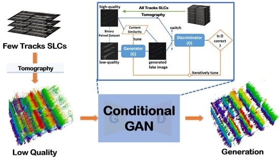
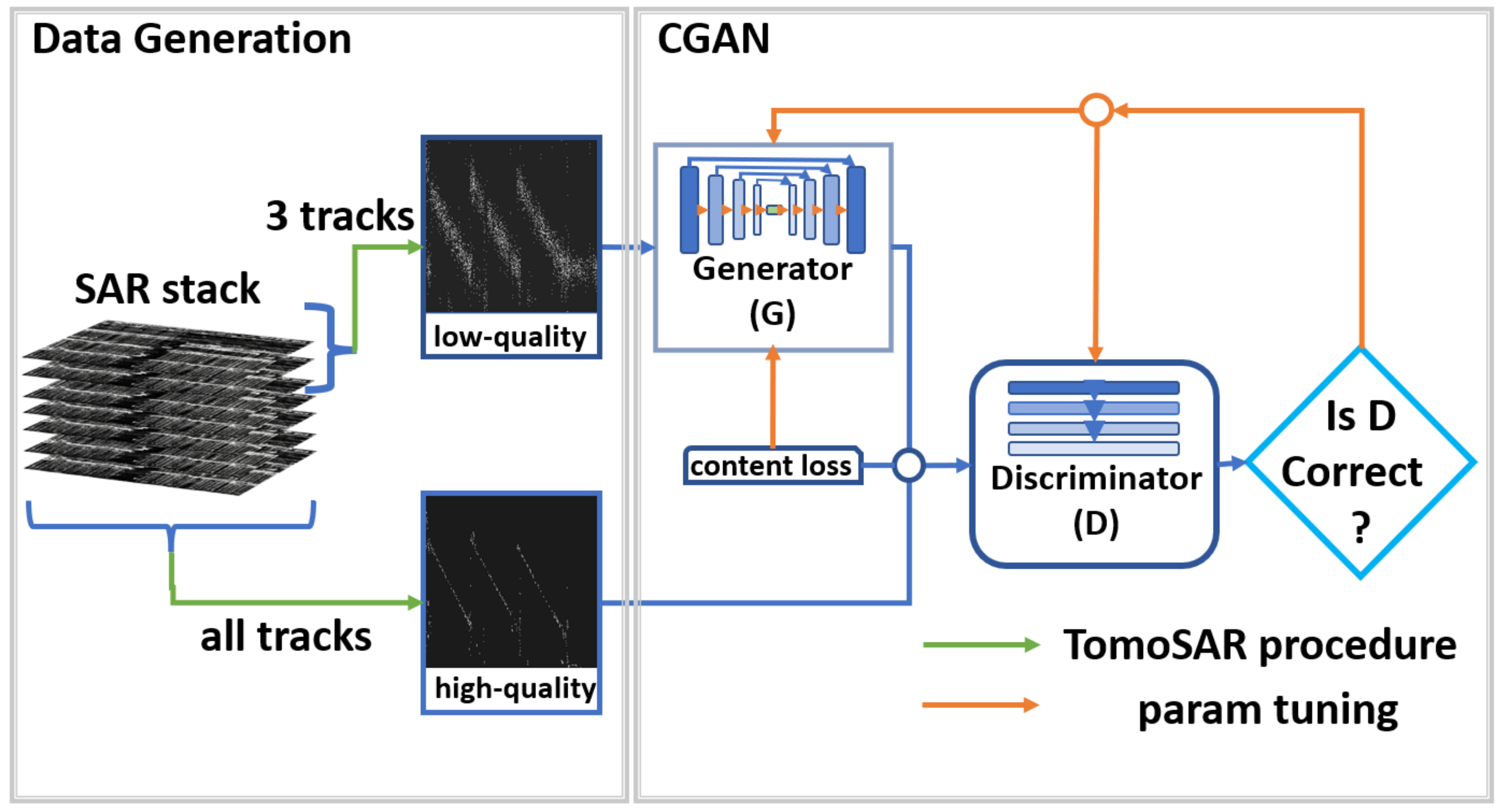
- The Conditional generative adversarial network (CGAN) is originally applied to generate high-quality TomoSAR 3D reconstruction for buildings using very few tracks by learning the high-dimensional features of architectural structures.
- (2)
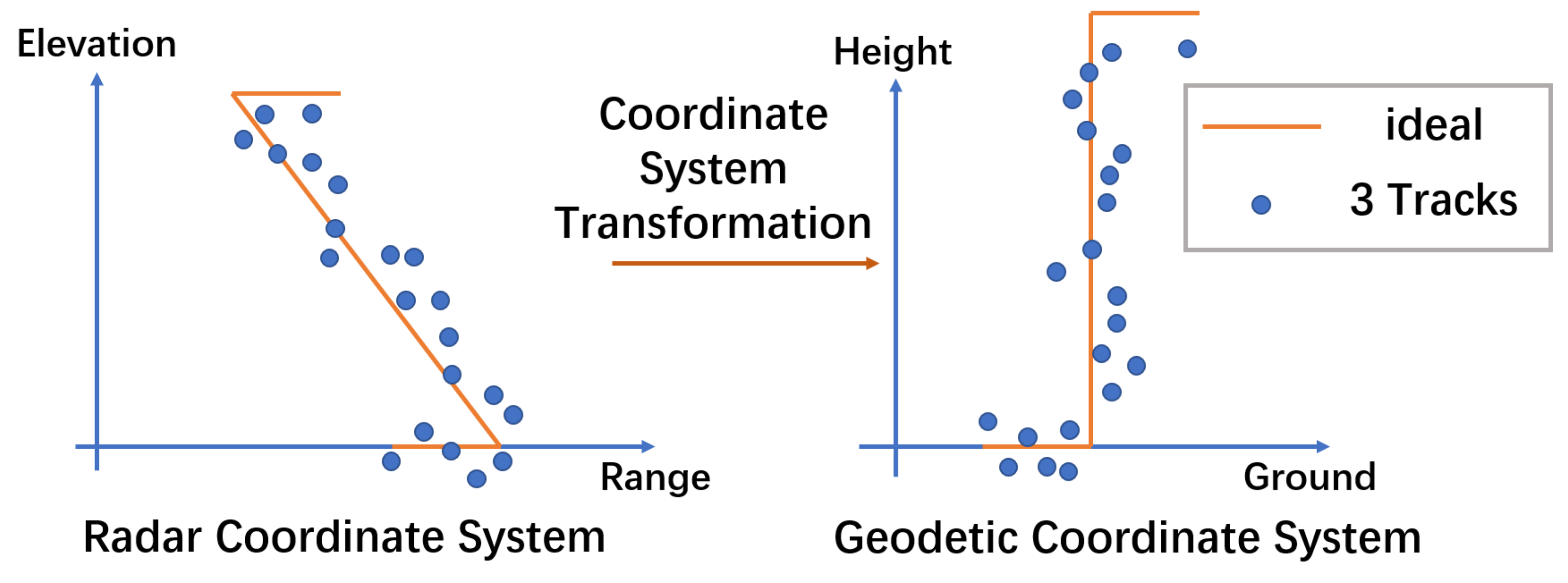
- Instead of directly processing large 3D data, the range-elevation 2D slices are processed to reduce network parameters and computational complexity, which makes it possible to deal with large-scale scenes. In order to solve the problem of possible misalignment among generations, the content loss between the input and generation is considered, so that the architectural structure can be reconstructed at the correct position.
- (3)
- The overlap of buildings in TomoSAR images makes buildings seem fused together and makes it hard to identify them from each other. The proposed method is able to distinguish the overlapped buildings correctly and estimate the heights of buildings. Compared with the widely used nonlocal algorithm, our method can estimate the height of buildings more accurately, and it is of higher time efficiency.
2. Materials and Methods
- Low-quality slice set: The low-resolution and low-SNR range-elevation slices generated using three tracks by TomoSAR procedure.
- High-quality slice set: The high-resolution and high-SNR range-elevation slices generated using all tracks.
2.1. Data Generation Module
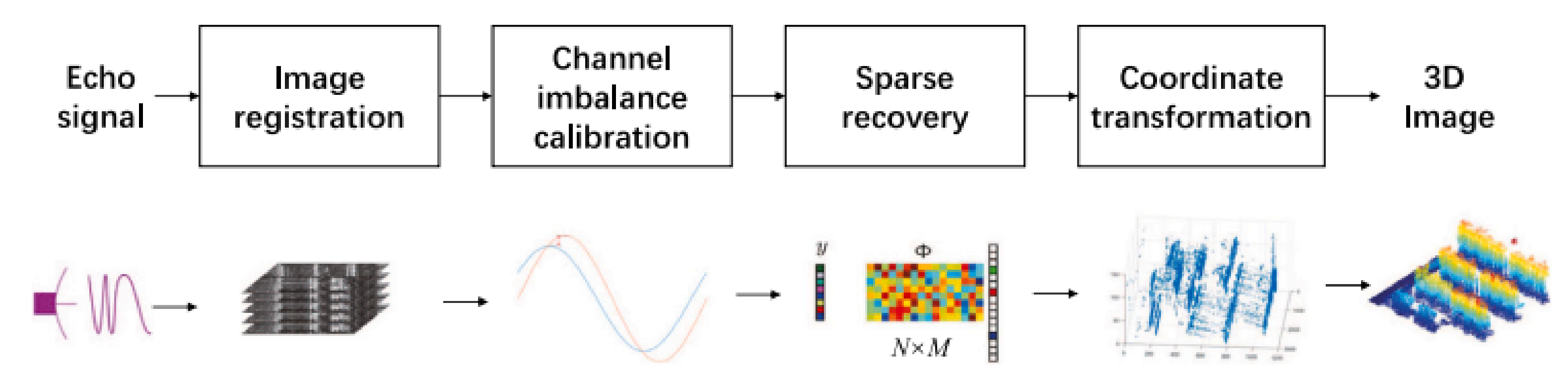
2.1.1. TomoSAR Principle
2.1.2. TomoSAR Procedure
2.1.3. Data Generation
2.2. CGAN Module
2.2.1. Generator
2.2.2. Discriminator
2.2.3. Loss Function
3. Results and Discussion
3.1. Network Training
3.2. Airborne Dataset
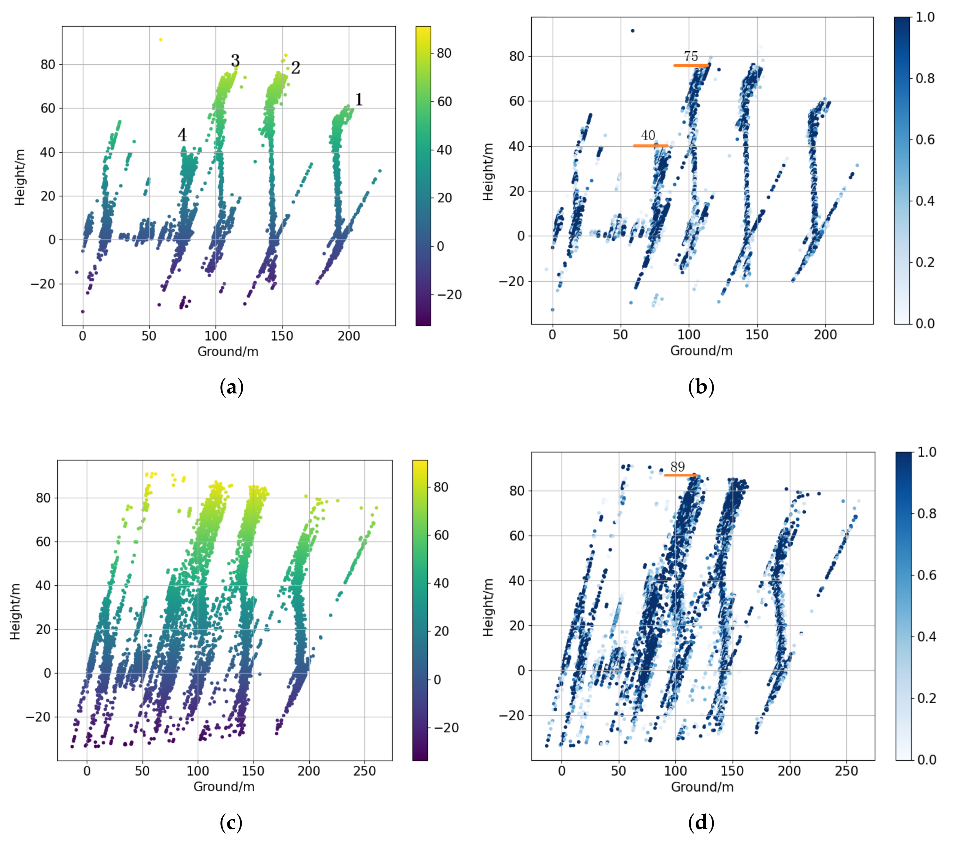
3.2.1. Nonoverlapped Buildings
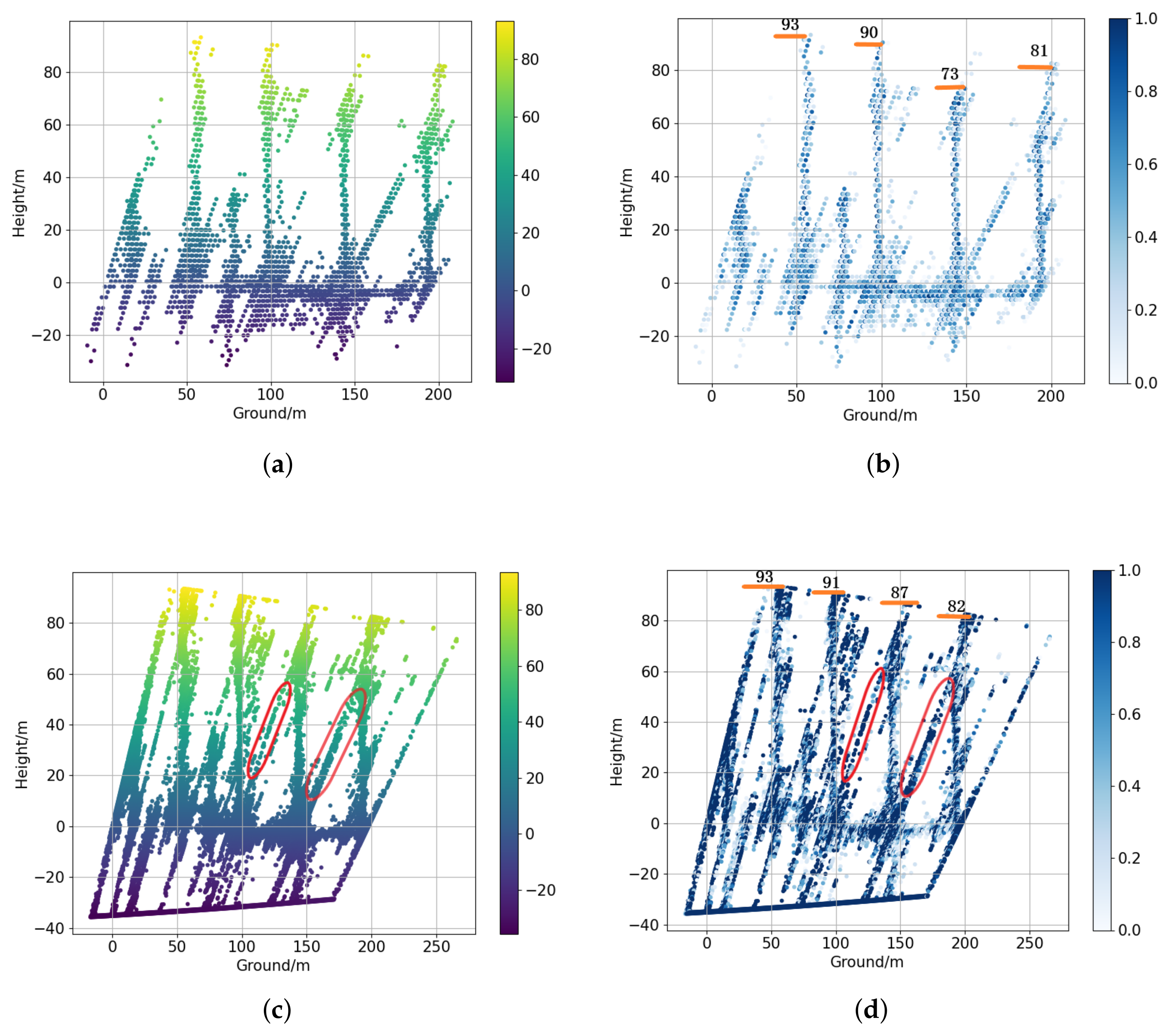
3.2.2. Overlapped Buildings
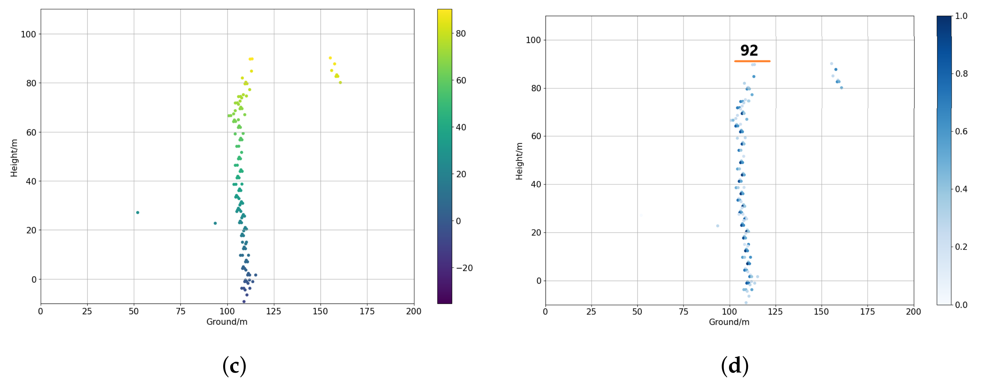
3.3. Spaceborne Dataset
4. Conclusions
Author Contributions
Funding
Institutional Review Board Statement
Informed Consent Statement
Data Availability Statement
Conflicts of Interest
References
- Reigber, A.; Moreira, A. First Demonstration of Airborne SAR Tomography Using Multibaseline L-Band Data. IEEE Trans. Geosci. Remote Sens. 2000, 38, 2142–2152. [Google Scholar] [CrossRef]
- Frey, O.; Meier, E. Analyzing Tomographic SAR Data of a Forest With Respect to Frequency, Polarization, and Focusing Technique. IEEE Trans. Geosci. Remote Sens. 2011, 49, 3648–3659. [Google Scholar] [CrossRef] [Green Version]
- Zhu, X.X.; Bamler, R. Very High Resolution Spaceborne SAR Tomography in Urban Environment. IEEE Trans. Geosci. Remote Sens. 2010, 48, 4296–4308. [Google Scholar] [CrossRef] [Green Version]
- Shi, Y.; Bamler, R.; Wang, Y.; Zhu, X.X. SAR Tomography at the Limit: Building Height Reconstruction Using Only 3–5 TanDEM-X Bistatic Interferograms. IEEE Trans. Geosci. Remote Sens. 2020, 58, 8026–8037. [Google Scholar] [CrossRef]
- Zhu, X.X.; Ge, N.; Shahzad, M. Joint Sparsity in SAR Tomography for Urban Mapping. IEEE J. Sel. Top. Signal Process. 2015, 9, 1498–1509. [Google Scholar] [CrossRef] [Green Version]
- Lu, H.; Zhang, H.; Deng, Y.; Wang, J.; Yu, W. Building 3-D Reconstruction With a Small Data Stack Using SAR Tomography. IEEE J. Sel. Top. Appl. Earth Obs. Remote Sens. 2020, 13, 2461–2474. [Google Scholar] [CrossRef]
- Zhou, S.; Li, Y.; Zhang, F.; Chen, L.; Bu, X. Automatic Reconstruction of 3-D Building Structures for TomoSAR Using Neural Networks. In Proceedings of the 2019 IEEE International Conference on Signal, Information and Data Processing (ICSIDP), Chongqing, China, 11–13 December 2019; pp. 1–5. [Google Scholar] [CrossRef]
- Wang, S.; Guo, J.; Zhang, Y.; Hu, Y.; Ding, C.; Wu, Y. Single Target SAR 3D Reconstruction Based on Deep Learning. Sensors 2021, 21, 964. [Google Scholar] [CrossRef]
- Goodfellow, I.J.; Pouget-Abadie, J.; Mirza, M.; Xu, B.; Warde-Farley, D.; Ozair, S.; Courville, A.; Bengio, Y. Generative Adversarial Networks. arXiv 2014, arXiv:1406.2661. [Google Scholar] [CrossRef]
- Radford, A.; Metz, L.; Chintala, S. Unsupervised Representation Learning with Deep Convolutional Generative Adversarial Networks. arXiv 2015, arXiv:1511.06434. [Google Scholar]
- Gulrajani, I.; Ahmed, F.; Arjovsky, M.; Dumoulin, V.; Courville, A. Improved Training of Wasserstein GANs. arXiv 2017, arXiv:1704.00028. [Google Scholar]
- Karras, T.; Laine, S.; Aila, T. A Style-Based Generator Architecture for Generative Adversarial Networks. arXiv 2019, arXiv:1812.04948. [Google Scholar]
- Wang, W.; Huang, Q.; You, S.; Yang, C.; Neumann, U. Shape Inpainting Using 3D Generative Adversarial Network and Recurrent Convolutional Networks. arXiv 2017, arXiv:1711.06375. [Google Scholar]
- Zhang, H.; Xu, T.; Li, H.; Zhang, S.; Wang, X.; Huang, X.; Metaxas, D. StackGAN: Text to Photo-Realistic Image Synthesis with Stacked Generative Adversarial Networks. arXiv 2017, arXiv:1612.03242. [Google Scholar]
- Brock, A.; Donahue, J.; Simonyan, K. Large Scale GAN Training for High Fidelity Natural Image Synthesis. arXiv 2018, arXiv:1809.11096. [Google Scholar]
- Tolosana, R.; Vera-Rodriguez, R.; Fierrez, J.; Morales, A.; Ortega-Garcia, J. DeepFakes and Beyond: A Survey of Face Manipulation and Fake Detection. arXiv 2020, arXiv:2001.00179. [Google Scholar] [CrossRef]
- Wang, X.; Han, S.; Chen, Y.; Gao, D.; Vasconcelos, N. Volumetric Attention for 3D Medical Image Segmentation and Detection. arXiv 2004, arXiv:2004.01997. [Google Scholar]
- Yu, Q.; Xia, Y.; Xie, L.; Fishman, E.K.; Yuille, A.L. Thickened 2D Networks for Efficient 3D Medical Image Segmentation. arXiv 2019, arXiv:1904.01150. [Google Scholar]
- Kupyn, O.; Budzan, V.; Mykhailych, M.; Mishkin, D.; Matas, J. DeblurGAN: Blind Motion Deblurring Using Conditional Adversarial Networks. arXiv 2018, arXiv:1711.07064. [Google Scholar]
- Zhu, X.X.; Bamler, R. Super-Resolution of Sparse Reconstruction for Tomographic SAR Imaging—Demonstration with Real Data. In Proceedings of the EUSAR 2012 9th European Conference on Synthetic Aperture Radar, Nuremberg, Germany, 23–26 April 2012; pp. 215–218. [Google Scholar]
- Zhu, X.X.; Bamler, R. Sparse Reconstrcution Techniques for SAR Tomography. In Proceedings of the 2011 17th International Conference on Digital Signal Processing (DSP), Corfu, Greece, 13–15 June 2011; pp. 1–8. [Google Scholar] [CrossRef]
- Zhu, X.X.; Adam, N.; Bamler, R. Space-Borne High Resolution Tomographic Interferometry. In Proceedings of the 2009 IEEE International Geoscience and Remote Sensing Symposium, Cape Town, South Africa, 12–17 July 2009; Volume 4, pp. IV–869–IV–872. [Google Scholar] [CrossRef]
- Jiao, Z.; Ding, C.; Qiu, X.; Zhou, L.; Chen, L.; Han, D.; Guo, J. Urban 3D Imaging Using Airborne TomoSAR: Contextual Information-Based Approach in the Statistical Way. ISPRS J. Photogramm. Remote Sens. 2020, 170, 127–141. [Google Scholar] [CrossRef]
- Fornaro, G.; Lombardini, F.; Pauciullo, A.; Reale, D.; Viviani, F. Tomographic Processing of Interferometric SAR Data: Developments, Applications, and Future Research Perspectives. IEEE Signal Process. Mag. 2014, 31, 41–50. [Google Scholar] [CrossRef]
- Xiang, Z.X.; Bamler, R. Compressive Sensing for High Resolution Differential SAR Tomography-the SL1MMER Algorithm. In Proceedings of the 2010 IEEE International Geoscience and Remote Sensing Symposium, Honolulu, HI, USA, 20–30 July 2010; pp. 17–20. [Google Scholar] [CrossRef] [Green Version]
- Weiß, M.; Fornaro, G.; Reale, D. Multi Scatterer Detection within Tomographic SAR Using a Compressive Sensing Approach. In Proceedings of the 2015 3rd International Workshop on Compressed Sensing Theory and Its Applications to Radar, Sonar and Remote Sensing (CoSeRa), Pisa, Italy, 17–19 June 2015; pp. 11–15. [Google Scholar] [CrossRef]
- Lie-Chen, L.; Dao-Jing, L. Sparse Array SAR 3D Imaging for Continuous Scene Based on Compressed Sensing. J. Electron. Inf. Technol. 2014, 36, 2166. [Google Scholar] [CrossRef]
- Guizar-Sicairos, M.; Thurman, S.T.; Fienup, J.R. Efficient Subpixel Image Registration Algorithms. Opt. Lett. 2008, 33, 156–158. [Google Scholar] [CrossRef] [PubMed] [Green Version]
- Isola, P.; Zhu, J.Y.; Zhou, T.; Efros, A.A. Image-to-Image Translation with Conditional Adversarial Networks. arXiv 2018, arXiv:1611.07004. [Google Scholar]
- Simonyan, K.; Zisserman, A. Very Deep Convolutional Networks for Large-Scale Image Recognition. arXiv 2015, arXiv:1409.1556. [Google Scholar]
- Cozzolino, D.; Verdoliva, L.; Scarpa, G.; Poggi, G. Nonlocal Sar Image Despeckling by Convolutional Neural Networks. In Proceedings of the IGARSS 2019–2019 IEEE International Geoscience and Remote Sensing Symposium, Yokohama, Japan, 28 July–2 August 2019; pp. 5117–5120. [Google Scholar] [CrossRef]
- Deledalle, C.A.; Denis, L.; Tupin, F. NL-InSAR: Nonlocal Interferogram Estimation. IEEE Trans. Geosci. Remote Sens. 2011, 49, 1441–1452. [Google Scholar] [CrossRef]
- D’Hondt, O.; López-Martínez, C.; Guillaso, S.; Hellwich, O. Nonlocal Filtering Applied to 3-D Reconstruction of Tomographic SAR Data. IEEE Trans. Geosci. Remote Sens. 2018, 56, 272–285. [Google Scholar] [CrossRef]
- Shi, Y.; Zhu, X.X.; Bamler, R. Nonlocal Compressive Sensing-Based SAR Tomography. IEEE Trans. Geosci. Remote Sens. 2019, 57, 3015–3024. [Google Scholar] [CrossRef] [Green Version]
- D’Hondt, O.; López-Martínez, C.; Guillaso, S.; Hellwich, O. Impact of Non-Local Filtering on 3D Reconstruction from Tomographic SAR Data. In Proceedings of the 2017 IEEE International Geoscience and Remote Sensing Symposium (IGARSS), Fort Worth, TX, USA, 23–28 July 2017; pp. 2476–2479. [Google Scholar]
- Cheng, R.; Liang, X.; Zhang, F.; Chen, L. Multipath Scattering of Typical Structures in Urban Areas. IEEE Trans. Geosci. Remote Sens. 2019, 57, 342–351. [Google Scholar] [CrossRef]


| All-Track | Three-Track | |
|---|---|---|
| Number of tracks | 8 | 3 |
| Maximal elevation aperture | 0.588 m | 0.168 m |
| Distance from the scene center | 1308 m | |
| Wavelength | 2.1 cm | |
| Incidence angle at scene center | 58° | |
| Parameter | Value |
|---|---|
| search window size | |
| patch size | |
| iterations | 10 |
| posterior similarity coefficient (h) | 5.3 |
| sparse prior KL similarity | |
| minimum number of similar blocks () | 10 |
| Building_Index | All Tracks | 3 Tracks\Error | Nonlocal\Error | Proposed\Error |
|---|---|---|---|---|
| #3 | 75 | 89\14 | 90\15 | 75\0 |
| #4 | 40 | Hard to recognize | 42\2 | 42\2 |
| #6 | 81 | 82\1 | 82\1 | 81\0 |
| #7 | 74 | 87\13 | 87\13 | 73\1 |
| #8 | 90 | 90\0 | 91\1 | 90\0 |
| #9 | 93 | 93\0 | 93\0 | 93\0 |
| Method | Time Consumption (s) |
|---|---|
| Nonlocal (10 iterations) | 14,492 |
| Proposed GAN | 10 |
| All-Track | Three-Track | |
|---|---|---|
| Number of tracks | 19 | 3 |
| Maximal elevation aperture | 215 m | 42 m |
| Distance from the scene center | 617 km | |
| Wavelength | 3.1 cm | |
| Incidence angle at scene center | 66° | |
Publisher’s Note: MDPI stays neutral with regard to jurisdictional claims in published maps and institutional affiliations. |
© 2021 by the authors. Licensee MDPI, Basel, Switzerland. This article is an open access article distributed under the terms and conditions of the Creative Commons Attribution (CC BY) license (https://creativecommons.org/licenses/by/4.0/).
Share and Cite
Wang, S.; Guo, J.; Zhang, Y.; Hu, Y.; Ding, C.; Wu, Y. TomoSAR 3D Reconstruction for Buildings Using Very Few Tracks of Observation: A Conditional Generative Adversarial Network Approach. Remote Sens. 2021, 13, 5055. https://doi.org/10.3390/rs13245055
Wang S, Guo J, Zhang Y, Hu Y, Ding C, Wu Y. TomoSAR 3D Reconstruction for Buildings Using Very Few Tracks of Observation: A Conditional Generative Adversarial Network Approach. Remote Sensing. 2021; 13(24):5055. https://doi.org/10.3390/rs13245055
Chicago/Turabian StyleWang, Shihong, Jiayi Guo, Yueting Zhang, Yuxin Hu, Chibiao Ding, and Yirong Wu. 2021. "TomoSAR 3D Reconstruction for Buildings Using Very Few Tracks of Observation: A Conditional Generative Adversarial Network Approach" Remote Sensing 13, no. 24: 5055. https://doi.org/10.3390/rs13245055
APA StyleWang, S., Guo, J., Zhang, Y., Hu, Y., Ding, C., & Wu, Y. (2021). TomoSAR 3D Reconstruction for Buildings Using Very Few Tracks of Observation: A Conditional Generative Adversarial Network Approach. Remote Sensing, 13(24), 5055. https://doi.org/10.3390/rs13245055