AVILNet: A New Pliable Network with a Novel Metric for Small-Object Segmentation and Detection in Infrared Images

Abstract

Infrared small-object segmentation (ISOS) has a persistent trade-off problem—that is, which came first, recall or precision? Constructing a fine balance between of them is, au fond, of vital importance to obtain the best performance in real applications, such as surveillance, tracking, and many fields related to infrared searching and tracking. F1-score may be a good evaluation metric for this problem. However, since the F1-score only depends upon a specific threshold value, it cannot reflect the user’s requirements according to the various application environment. Therefore, several metrics are commonly used together. Now we introduce F-area, a novel metric for a panoptic evaluation of average precision and F1-score. It can simultaneously consider the performance in terms of real application and the potential capability of a model. Furthermore, we propose a new network, called the Amorphous Variable Inter-located Network (AVILNet), which is of pliable structure based on GridNet, and it is also an ensemble network consisting of the main and its sub-network. Compared with the state-of-the-art ISOS methods, our model achieved an AP of 51.69%, F1-score of 63.03%, and F-area of 32.58% on the International Conference on Computer Vision 2019 ISOS Single dataset by using one generator. In addition, an AP of 53.6%, an F1-score of 60.99%, and F-area of 32.69% by using dual generators, with beating the existing best record (AP, 51.42%; F1-score, 57.04%; and F-area, 29.33%).

1. Introduction

Infrared small-target applications are widely exploited in many fields such as maritime surveillance [1,2,3,4], early warning systems [5,6,7], tracking [8,9,10,11,12,13], and medicine [14,15,16,17,18], to name but a few. Heat reveals a critical salient characteristic in the local background of infrared images, and it could be a conclusive, distinct clue for effortless object segmentation. Nevertheless, infrared small-object segmentation (ISOS) is a challenging task because heavy background clutters and sensor noise as shown in Figure 1. Suppose local patch-based ISOS handcraft methods [19,20,21] perform the segmentation task in those scenarios, i.e., under heavy clutter or sensor noise. What happens next in the confidence map? Essentially, this gives rise to umpteen false alarms from employing too narrow a receptive field, perceiving local visual-context information, and using too few filters when learning from several cases. Therefore, that condition makes it hard to distinguish the foreground from various complex background patterns.

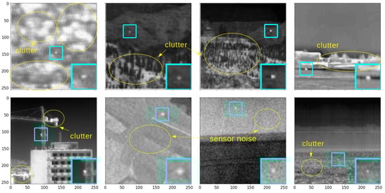
Figure 1. Infrared small-object samples. A lot of background clutter and sensor noise distorts the objects of interest.

Viewed in this light, the performance in the ISOS task is contingent on the learning ability, that how well it distinguishes out the complex background patterns surrounding the objects of interest, and not the objects themselves. Specifically, this tendency occurs more often from following three major characteristics of infrared small objects. First, owing to either a long distance from the sensor or its actual size, the object appears very small in the image and its inner pattern convergences to one point. This phenomenon makes almost all category classification impossible. Second, following the first effect, if objects have similar shapes, instance classification is not reliable anymore. Third, when two or more objects overlap, they may appear as one object. That is a fatal constraint if we must separate them into different instances.

Incidentally, at the pixel level, these three characteristics reduce the difference in the task between small-object segmentation and detection from the vantage point of the ISOS task. That is why we include detection in this paper’s title. To enhance understanding, let us presume a drastic, but practical example. Wang et al. [22] published the ISOS Single dataset at the International Conference on Computer Vision (ICCV). That dataset has some sparse images that have only one object, sized at 1 pixel by 1, in one image. Suppose the two tasks (i.e., segmentation and detection) perfectly perform their operations on the same image satisfying the above case. The objects, separated from the background in the results, must be exactly the same as each other. As a result, the segment which is yielded from the bounding box surrounding the object has a size of 1 pixel by 1. The size is the same compared to the segmentation result. Starting from this perspective, we can compare the state-of-the-art (SOTA) detection method, i.e., YoloV4 [23].

As a result that the object in the image is so small, an understanding of context (comprised of the pixels surrounding the object) works as a critical proviso, more so than the shape of the object itself. This fact shows that methods based on a convolutional neural network (CNN), which consist of numerous filters for training various patterns, surpass the handcraft-based methods. DataLossGAN [22] is a CNN-based method. It exploits two generators, assigning different opposite objectives to obtain a delicate balance between missed detection (MD) and false alarm (FA). This strategy was greatly effective, and sufficient to set up the SOTA ICCV2019 ISOS Single dataset.

The whole DataLossGAN [22] structure is comprised of several plain networks as shown in Figure 2. As a result that the two generators are constructed with a few shallow layers, DataLossGAN [22] must go through quite a few iterations to find the global optimum in the manifold background patterns. These dual-learning systems have a non-immediate connection to each other so that, indirectly, they depend on only L1-distance at the feature level via the discriminator to regulate the delicate balance between MD and FA. Consequentially, these dual-learning systems succeed in obtaining a high score for average precision (AP), but a low F1-score. Specifically, the one generator only concentrates on decreasing MD, while the other only concentrates on decreasing FA, and as the discriminator endeavors to reduce the difference in the inclination between the two generators, it is overly indirect.

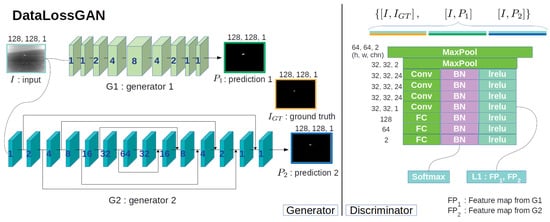
Figure 2. Model overview of DataLossGAN International Conference on Computer Vision (ICCV) 2019 [22]: On the left are two generators (G1 and G2), and on the right is one discriminator. In the two generators, the blue number within each layer is the dilation factor. For the discriminator, the height, width, and channel number of the output feature maps are marked beside each layer. The two generators compose the dual-learning system concentrating on opposing objectives while sharing information (e.g., L1-distance between G1 and G2 feature maps) with the discriminator to alleviate radical bias training.

We hypothesize that one generator is more efficient than two in terms of direct information interchange via perceptrons for one goal, i.e., ISOS. At the end of various analytical experiments, we succeed in obtaining what we call the Amorphous Variable Inter-located Network (AVILNet). This successful network harmoniously tunes the balance between recall and precision quite well.

AVILNet is comprised of various methods following the latest fashions, that achieved the SOTA in each of their fields, e.g., GridNet [24], Cross-Stage-Partial-Net (CSP-Net) [25], atrous convolution [26] (dilation convolution), and Dense-Net [27]. Aside from that, other related methods are exploited for the various experiments in Section 5.2. The contributions of this paper can be summarized as follows.

(1) We introduce AVILNet, inspired by GridNet [24]. This deep CNN was designed for its increasing learning ability, and for distinguishing the foreground from a complicated background. In addition, this network finds the global optimum very quickly (within two epochs). It means AVILNet may provide better performance with more extensive training data. To alleviate the gradient vanishing problem which is intensified by a complex deep structure, we adopted CSP-Net [25] with dilation convolution [26] in AVILNet.

(2) To obtain a suitable model and establish its validity, we performed various experiments, step by step, building a hypothesis and confirming it. Plenty of experiments show that our method was achieved elaborately, not by coincidence.

(3) We discreetly introduce the novel metric F-area, which multiplies AP by the best F1-score. It is a trustworthy metric when true negatives are greater than 99% in an image, compared to area under the receiver operating characteristic (ROC) curve (AUC). In addition, it simultaneously considers performance in terms of real application and potential capability.

(4) We compared AVILNet with relevant state-of-the-art small-object segmentation methods on public data from ICCV2019 ISOS. The results demonstrate the superiority of AVILNet, beating the existing best record.

2. Related Work

ISOS methods can generally be categorized into two groups, depending on whether they are CNN-based or not. Recently, fully connected network (FCN) [28] based methods have been applied to ISOS [7,22,29,30,31]. In particular, DataLossGAN [22] and Asymmetric Contextual Modulation (ACM) [31] have obtained magnificent performance on their datasets. Meanwhile, handcraft-based methods [6,20,21,32,33,34,35,36,37,38] have also been studied. Researchers have analyzed local properties in scenes to distinguish the foreground from the background, patch by patch, and have applied a few well-designed filters to whole images in a sliding window manner. Both groups, finally, adopt a mono- or adaptive-threshold policy to produce a gray scale confidence map.

In this section, we briefly pinpoint and visit the few properties and problems for ISOS in terms of CNN structures with related successful studies.

2.1. Deeper Network vs. Vanishing Gradient

In a broad sense, the ISOS task is classified into two objectives. The first is background suppression; the second is intensification of the objects of interest. Most traditional approaches [6,20,21,32,33,34,35,36,37,38] execute the two objectives sequentially with only a few filters, which are elicited through human analysis. CNN-based methods perform the whole task under latent space comprised of numerous parameters in the network regardless of the sequence. Each kernel of a CNN, as a unique filter, is aimed at suppressing background clutter or sensor noise, or to enhance the object of interest.

Consequently, owing to the limits of manual methods, the handcraft-based methods construct only a few filters by observing several cases. This strategy gives rise to a phenomenon whereby generalization performance is decided from the rules, by which the training data determine how well the selected cases represent the distribution of all the test data.

In comparison, the CNN-based methods [7,22,29,30,31] have numerous filters, which are sufficient to cover the distribution of all the test data. This is why the CNN is superior in terms of absolute performance measure, than the handcraft-based methods.

The capacity of the filters affects the performance of ISOS. Simultaneously, it increases the probability of incurring the vanishing gradient problem. To alleviate this phenomenon, there have been many studies in terms of architecture methodology, e.g., HighwayNet [39], ResNet [40], ResNext [41], Drop out [42], GoogleNet [43], and DenseNet [27].

2.2. Attention and the Receptive Field

A deeper network, comprised of multi-layers, could be a solution for increasing the learning capability. However, it is too hard to preserve the features of small infrared objects in deep layers, so that re-awakening strategies, which remember prior or low-level layer feature information, have been studied [24,31,44,45].

Luong et al. [44] proposed global and local attention for neural machine translation. The global attention takes all prior memories and the local attention takes several prior memories at a current prediction. In the computer vision, generally these attention concepts have been utilized in a slightly different way. The global attention refers to all prior feature maps, but the local attention refers to several prior feature maps to a current layer. The definition of receptive field is the size of the region in the input that produces the feature map [46].

In segmentation, deep CNNs should be able to access all the relevant parts of the object of interest to understand context. That is why multi-scale approaches are commonly taken to accelerate the performance [24,31,45,47].

GridNet [24] exploits a grid organization with a two-dimensional architecture for multi-scale attention. The grid organization has two advantages for architecture. The one is that GridNet can simultaneously consider the problem of setting the attention and the receptive field by two parameters (i.e., width and height). The other is that GridNet follows the rule of grid, so the produced model meets always a grid shape. The second advantage makes less an effort to set the detailed configuration for layers.

Furthermore, GridDehazeNet [45] ameliorates GridNet by replacing the residual block [40] with a dense block [27], and replacing simple addition with attention-based addition at each confluence in the network.

Chen et al. [48] successfully adopted dilation convolution of the semantic segmentation field [26]. Its benefit is that it does not increase the computational parameters, but spreads the receptive field, and concomitantly alleviates lattice patterns caused by overlap accumulation. Dai et al. [31] proposed the ACM for ISOS. This module takes a two-directional path (top-down and bottom-up) to preserve prior feature information.

We analyzed GridNet [24] for diverse experiments because of its pliable structure. Furthermore, GridDehazeNet [45] was chosen as the baseline.

2.3. Data-Driven Loss and Ensemble

DataLossGAN [22] proposed data-driven loss to obtain a delicate balance between MD and FA. DataLossGAN consists of two generators, in which they concentrate on mutually incompatible objectives, and in the test phase, decision making is done in an ensemble manner. This study inspired us, so that AVILNet adopts both data loss and the ensemble manner. However, in our case, we construct a sub-network within the main network. A detailed explanation is in Section 3.2.2.

2.4. Generative Adversarial Network

A generative adversarial network consists of two parts: a generative network (generator) and a adversarial network (discriminator) [49]. In the training step, the goal of the generator is to learn to generate fake data following the distribution of real data. Meanwhile, the aim of the discriminator is to learn to distinguish between fake data and real data.

Auto-encoder is a generalized approach for image-to-image segmentation [47,50,51]. If an auto-encoder is considered as one generator, a generative adversarial network is available. Especially, in our case, $inputvectorZ\sim latentspace$ is replaced with $inputvectorZ\sim$${\mathbb{R}}^{W,H,C}$, so that the whole model can be regarded as conditional GAN (cGAN) [52].

DataLossGAN [22] also used this methodology and exploited a discriminator to mitigate the output difference between two generators. Our proposed training strategy dose not share the outputs via the discriminator, but has direct connections within the generative network.

Our generative network can be divided into two networks. One is the main network and the other is the sub-network. Therefore, the generative network operates as an ensemble manner for the final decision making the confidence map.

2.5. Resizing during Pre-Processing

Generally, most CNN-based semantic segmentation studies have focused on commercial usage [48,53]. Therefore, they do not need to consider small-sized objects within a small image. This history leads to resizing the input image to go through a large-scale backbone for small-object applications [31,54,55]. In the field of ISOS, ACM [31] adjusts the size of the input image to $512\times 512$, and then, randomly crops one segment, which has a size of $480\times 480$, from within the whole image area. On the other hand, DataLossGAN [22] adopted a patch training strategy in which input patches are sized at $128\times 128$. We experimented with both the above strategies to make an impartial observation of each effect.

3. The Proposed Method

This section discusses handling the above issues with our approach. After that, our proposed model overview is shown. Following that, details of the structure and the loss function are presented.

3.1. Our Approach

To find the solution for ISOS, we conducted an experiment to determine what architecture is truly proper for ISOS. Most backbone research, unfortunately, was performed on the assumption that a large-scale object is in a large image [40,56]. In addition, the laminated backbone structure is not pliable enough for executing experiments with various configurations. For this reason, our first objective was finding a flexible backbone for a varied receptive field or multi-scale attention, either way. The GridNet [24] structure perfectly corresponds to the objective as shown in Figure 3. We set GridDehazeNet [45] with a modified loss function as our initial study due to fact that they published their clean code. GridDehazeNet is based on GridNet, too, but replaces feature addition with attention-based addition. This method boosts performance. The difference between D8 and D17 in Table 1 is only that of exploiting attention-based addition or not. Therefore, we set the GridDehazeNet as the baseline.

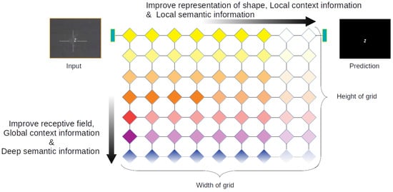
Figure 3. AVILNet is inspired by GridNet [24]. This ’grid’ structure is extremely pliable. In terms of network perception, the horizontal stream (black arrow pointing right) enforces local properties and the vertical stream (black arrow pointing downward) enforces global properties. To transform the grid structure, we only have to set the two parameters (’width’ and ’height’).

Table 1. Ablation study for diverse hyper-parameters and strategies on the ICCV 2019 infrared small-object segmentation (ISOS) Single dataset. In these experiments, we set st at 36, except for D1 (st = 8) and D8 (st = 34). D12 did not adopt the CSP [25]. D17 replaced attention-based feature addition with feature addition and D18 replaced the mish activation function with leaky ReLU (0.2) compared to D8. The bold denote the best scores.

Index	gw	nd	w	h	RS	lr	$\mathit{l}2$	DL	L	SF	${\mathit{\lambda }}_{\mathbf{MD}},{\mathit{\lambda }}_{\mathbf{FA}}$	ep	F1	AP	AUC	Fa
D1	16	4	3	6	1	${10}^{-4}$	✓	✓	✓		100, 10	123	0.564	0.486	0.799	0.274
D2	8	7	3	6	1	${10}^{-4}$		✓	✓		100, 10	23	0.561	0.495	0.783	0.278
D3	8	7	3	6	3	${10}^{-4}$		✓	✓		100, 10	76	0.601	0.503	0.793	0.302
D4	8	7	3	6	3	${10}^{-4}$	✓	✓	✓		100, 10	4	0.564	0.485	0.785	0.236
D5	8	7	6	3	3	${10}^{-4}$		✓	✓		100, 10	51	0.570	0.494	0.799	0.282
D6	8	7	6	3	3	${10}^{-4}$		✓			100, 10	4	0.594	0.441	0.726	0.251
D7	8	7	6	3	3	${10}^{-3}$		✓	✓		100, 10	24	0.554	0.437	0.729	0.242
D8	24	7	4	6	3	${10}^{-4}$	✓	✓	✓		100, 10	2	0.630	0.517	0.832	0.326
D9	24	7	4	6	3	${10}^{-4}$	✓	✓	✓	(b)	100, 10	17	0.576	0.496	0.789	0.286
D10	24	7	4	6	3	${10}^{-4}$	✓	✓	✓	(c)	100, 10	31	0.575	0.477	0.790	0.279
D11	24	7	4	3	3	${10}^{-4}$	✓	✓	✓		100, 10	5	0.574	0.440	0.740	0.252
D12	24	7	4	6	3	${10}^{-4}$	✓				100, 10	26	0.552	0.448	0.753	0.247
D13	24	7	4	6	3	${10}^{-5}$	✓	✓	✓		100, 10	3	0.546	0.449	0.779	0.245
D14	24	7	4	6	3	$0.5\times {10}^{-4}$	✓	✓	✓		100, 10	3	0.560	0.475	0.798	0.266
D15	24	7	4	6	3	${10}^{-5}$	✓	✓	✓		100, 3	3	0.563	0.486	0.782	0.273
D16	24	7	4	6	3	${10}^{-4}$	✓	✓	✓		100, 3	19	0.564	0.470	0.771	0.265
D17	24	7	4	6	3	${10}^{-4}$	✓	✓	✓		100, 10	2	0.581	0.485	0.790	0.282
D18	24	7	4	6	3	${10}^{-4}$	✓	✓	✓		100, 10	10	0.593	0.507	0.849	0.301
D19	24	7	4	6	2	${10}^{-4}$	✓	✓	✓		100, 10	5	0.575	0.522	0.817	0.300
D20	24	7	4	6	1	${10}^{-4}$	✓	✓	✓		100, 10	5	0.566	0.495	0.801	0.280
D21	24	7	4	6	3	${10}^{-4}$		✓	✓		100, 10	2	0.581	0.455	0.782	0.264

3.2. The Amorphous Variable Inter-Located Network

In this subsection, we do not deal with the experiments in detail, but concentrate on AVILNet itself. As illustrated in Figure 4, AVILNet consists of one generator and a discriminator, like cGAN [52]. It is a common strategy, but the inner architecture of the generator is novel. Our most valuable choice was adopting a grid structure as the development backbone. The greatly pliable organic architecture led us to various experiments. As shown in Table 1, AVILNet (denoted as D8) was obtained after plenty of attempts. Increasing the $width$ of the generator improves the representational ability of the shape, the local context, and the semantic information. Conversely, $height$ improves the receptive field, the global context, and the deep semantic information. As a consequence, AVILNet is flexible in responding to the given task by changing $height$ and $width$. In short, AVILNet is amorphous and variable.

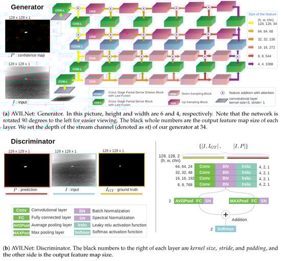
Figure 4. The whole architectural overview of AVILNet (as proposed).

3.2.1. Cross-Stage Partial Dense Block and Dense Dilation Block

The Q1 baseline only use a dense block [27]. Due to the duplicate gradient information [25], it wanders in the local minimum. The details of Q1 are shown in Table 2. To overcome this problem, we apply the cross-stage partial strategy (CSP) to the dense block of Q1. Therefore, it is called the cross-stage dense block (CDB). The original CSP strategy, which records the best performance on a large-scale object dataset [57], showed rather poor performance compared to the last-fusion strategy in our case. This is because a secondary transition layer distorts the feature information of a small object. We tackle this issue by changing the original CSP with last-fusion within the CDB. Furthermore, following successful application of dilation convolution [22,48], we propose the cross-stage partial dense dilation block with last-fusion (CDDB-L) as shown in Figure 5. This boosts our task from the suitable usage proportion.

Table 2. Ablation study, step by step, in terms of the discriminator, the activation function, the extension of gw and nd, CSP strategies, dilation, and the blocks (Dense, Res, ResNext). The baseline Q1 set the gw and nd at 16 and 4, respectively. The bold denote the best scores.

Index	Data Loss	Discriminator	Mish	gw + nd	ori	lafu	DL	Dense	Res	ResNext	ep	F1	AP	AUC	Fa
Q1	✓							✓			11	0.515	0.390	0.731	0.201
Q2	✓	✓						✓			7	0.526	0.413	0.792	0.217
Q3	✓	✓	✓					✓			8	0.534	0.426	0.786	0.227
Q4	✓	✓	✓	✓				✓			4	0.509	0.399	0.724	0.203
Q5	✓	✓	✓	✓	✓			✓			14	0.591	0.519	0.792	0.307
AVILNet (Single)	✓	✓	✓	✓		✓	✓	✓			2	0.630	0.517	0.832	0.326
AVILNet (Dual)	✓	✓	✓	✓		✓	✓	✓			1	0.610	0.536	0.928	0.327
Q6	✓	✓	✓	✓					✓		22	0.586	0.464	0.801	0.272
Q7	✓	✓	✓	✓						✓	15	0.576	0.460	0.774	0.265

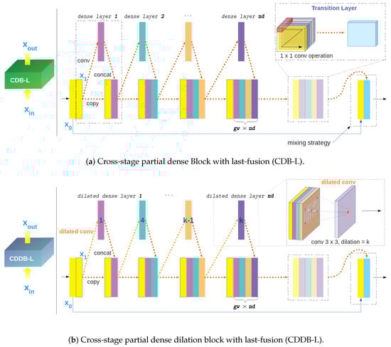
Figure 5. Detailed overviews of CDB-L and CDDB-L. Unlike the study in [25], we take the last-fusion strategy where, in the final processing, addition is modified to concatenation. The dilation layer in CDDB-L improves the quality of the segmentation task through alternative sampling [48]. The ablation study for observing the effects of diverse strategies is shown in Table 2. The blue number within the layer is the dilation factor.

The growth and the number of dense layers in CDB-L or CDDB-L are decided by the hyper-parameter gw and nd. The dilation factor at the $\theta$th layer in CDDB-L is calculated as

$$when\theta \in \left\{1,2,3,\dots ,\mathrm{nd}\right\}\mathrm{the}\mathrm{dilation}\mathrm{factor}k=2^{\theta -1}$$

(1)

3.2.2. Multi-Scale Attention-Based Ensemble Assistant Network and Feature-Highway Connections

One of the main contributions is that we successfully analyzed the feature-highway connections and formulated its structure. The overview of feature-highway connections is shown in Figure 6. Following the last-fusion strategy, feature-highway connections are consequentially built within the generator to flow information smoothly without congestion. In particular, it works to assist the regularization of object shape and context at the final decision in an ensemble manner, like ResNext [41]. The equations representing the above theory can be expressed as follows.

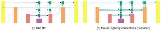
Figure 6. To explain the difference between GridNet [24] and our methods, we illustrate the information flow of them. (a) GridNet, and (b) the feature-highway connections (blue arrows). This allows the information to flow through the down-sampling block (DSB) and the up-sampling block (USB), like a grid pattern, without entering the transition layer.

Let $\zeta$, x, and y be the group residual block, the input, and output, respectively:

$$y=x+\sum _{i=1}^C{\zeta }_i\left(x\right)i=0,1,2,\dots ,CCiscardinality$$

(2)

Equation (2) explains one ResNext [41] block formula. Then, our generator denotes $height$ and $width$ as h and w, respectively. In addition, in a CDB-L or CDDB-L, the feature maps of the generator in a stage are split into two parts through channel $x=[x_0,x_1]$. The $x_0$ undergoes the feature-highway connections, and $y_0$ is the output from the connections. In that case, we can set $a_{i,j}$, $D_{i,j}$, $b_{i,j}$, $U_{i,j}$, x, and y to denote a feature vector corresponding to the $i,j$ coordinates down-stream, to denote the down-sampling block (DSB), a feature vector corresponding to $i,j$ coordinates up-stream, an up-sampling block (USB), input, and output, respectively. For simplicity, we leave out the weighted sum operation, and we replace symbols of the $x_0,y_0$ with $x,y$. Note that the $i,j$ coordinates indicate each addition confluence of the grid. Details on the DSB and the USB are shown in Figure 7. Following that, our feature-highway connections can be expressed as:

$$\begin{array}{c}\hfill \begin{array}{c}\hfill \mathrm{On}\mathrm{downstream},\\ \hfill a_{11}& =D_{11}\left(x\right)\hfill \\ \hfill a_{12}& =a_{11}+D_{12}\left(x\right)\hfill \\ \hfill & .\hfill \\ \hfill a_{1,w/2}& =a_{1,w/2-1}+D_{1,w/2}\left(x\right)\hfill \\ \hfill & .\hfill \\ \hfill a_{h-1,w/2}& =a_{h-1,w/2-1}+D_{h-1,w/2}\left(a_{h-2,w/2}\right)\hfill \end{array}\end{array}$$

(3)

$$\begin{array}{c}\hfill \begin{array}{c}\hfill \mathrm{On}\mathrm{upstream},\\ \hfill b_{h-1,w/2+1}& =a_{h-2,w/2}+U_{h-1,w/2+1}\left(a_{h-1,w/2}\right)\hfill \\ \hfill b_{h-1,w/2+2}& =b_{h-1,w/2+1}+U_{h-1,w/2+2}\left(a_{h-1,w/2}\right)\hfill \\ \hfill & .\hfill \\ \hfill b_{h-1,w}& =b_{h-1,w-1}+U_{h-1,w}\left(a_{h-1,w/2}\right)\hfill \\ \hfill b_{h-2,w}& =b_{h-2,w-1}+U_{h-2,w}\left(b_{h-1,w}\right)\hfill \\ \hfill & .\hfill \\ \hfill b_{1,w/2+1}& =x+U_{1,w/2+1}\left(b_{2,w/2+1}\right)\hfill \\ \hfill b_{1,w/2+2}& =b_{1,w/2+1}+U_{1,w/2+2}\left(b_{2,w/2+2}\right)\hfill \\ \hfill & .\hfill \\ \hfill b_{1,w}& =b_{1,w-1}+U_{1,w}\left(b_{2,w}\right)\hfill \\ \hfill y=b_{1,w}& =x+U_{1,w/2+1}\left(b_{2,w/2+1}\right)\cdots +U_{1,w}\left(b_{2,w}\right)\hfill \end{array}\end{array}$$

(4)

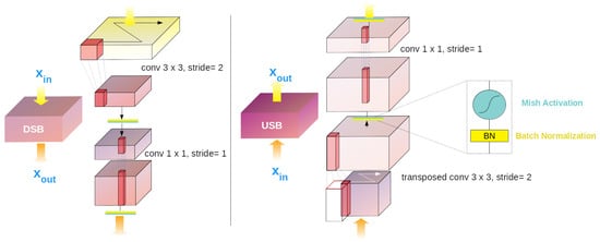
Figure 7. Detailed overviews of the down-sampling block (DSB) and the up-sampling block (USB). Instead of simple binary up-sampling, two convolutional processes operate. This strategy makes our feature-highway connections trainable.

Finally, we get Equation (5):

$$\begin{array}{c}\hfill \begin{array}{cc}\hfill y& =x+\sum _{i=w/2+1}^w{U}_{1,i}\left(b_{2,i}\right)i=w/2,w/2+1,\dots ,w-1,w\hfill \end{array}\end{array}$$

(5)

Following Equation (5), we can illustrate the overview of our proposed method, i.e., a multi-scale attention-based ensemble assistant network (MEN), as shown in Figure 8. This obtained latent network gives us profound insight into how our generator preserves the low-level information of small objects at a high level without any short connections. In comparison to ResNext [41], the MEN has attention-based flow, which is represented by the interconnected black lines in Figure 8. It encourages inter-exchange of semantic information between each decision group. In addition, ResNext [41] performs in an ensemble manner by through channel-wise grouping, but our method exploits all the channels. The former obtains an advantage in terms of reducing computational resources, but the blocks ($\zeta$), have nothing to communicate to each other. ResNext [41] concentrates on improving performance at the decision level in an ensemble manner, rather than an attention manner. On the other hand, our generator has much smaller cardinality (ResNext [41] set the cardinality at 32 by default, but our generator set the cardinality at 2.) than the former, while having plentiful inter-connections for attention. As shown in Table 3, the results of the experiment verify that our method (MEN) is more suitable for the ISOS task. To sum up, we regard the MEN as a sub-network supporting the main network.

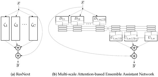
Figure 8. Illustrated are (a) ResNext [41] and (b) our assistant network, which has a multi-scale attention-based ensemble decision system with feature-highway connections.

Table 3. Comparison of MEN and ResNext. The bold denote the best scores.

Sub-Network	Setting	ep	F1	AP	AUC	Fa
MEN (Proposed)	D8	1	0.630	0.517	0.832	0.326
ResNext	D8	1	0.560	0.433	0.721	0.243

3.2.3. Over-Parameterization

Allen-Zhu et al. [58] explained the relationship between network parameters and learning convergence time. In detail, they suggested that if input data do not degenerate, i.e., $anyx\in {\mathbb{R}}^{dim},x_i\ne x_{j}wherei\ne j$, and the network is over-parameterized, it can indeed be trained by regular first-order methods (e.g., SGD) to the global minima. This theorem can be expressed as follows:

$$\begin{array}{c}\hfill \begin{array}{cc}\hfill \mathrm{In}\mathrm{convolut}& \mathrm{ion}\mathrm{neural}\mathrm{networks}\dots \hfill \\ \hfill T& =\tilde{O}\left(\frac{poly(n,L,\mathfrak{d})}{{\delta }^2}·\log {\epsilon }^{-1}\right)\hfill \end{array}\end{array}$$

(6)

where T is the number of iterations; $\tilde{O}$ is the symbol for time complexity; $n,L,and\mathfrak{d}$ are the number of samples in the training dataset, the number of layers, and the number of pixels in the feature maps; $\delta$ denotes the relative distance between two training data points, and $\epsilon$ is the objective error value. Furthermore, Allen-Zhu et al. [59] compared the relationship between the number of layers and hidden neurons. Following the two conclusions, our AVILNet generator is designed to have many more trainable parameters and layers than other state-of-the-art methods. Thanks to this strategy, our method obtains wonderful convergence speed, as shown in Table 4. AVILNet educes maximum performance within two epochs.

Table 4. Comparison of state-of-the-art methods. The bold denote the best scores for each indicator.

Method	FLOPs	Parameters	ep	F1	AP	AUC	Fa	Framework
AVILNet (Single)	10.98B	90.98M	2	0.630	0.517	0.832	0.326	Pytorch
AVILNet (Dual)	21.96B	161.96M	1	0.610	0.536	0.928	0.327	Pytorch
DataLossGAN	30.89B	3.14M	29	0.577	0.514	0.834	0.293	Pytorch
ACM-FPN	0.565B	0.387M	91	0.616	0.475	0.803	0.293	Pytorch
ACM-UNet	0.9B	0.520M	38	0.568	0.422	0.821	0.240	Pytorch
YoloV4	31.05B	20.6M	21	0.503	0.356	0.851	0.184	Pytorch
DeepLabV3	44.425B	59.34M	11	0.105	0.026	0.124	0.003	Pytorch
IPI	’	’	’	0.449	0.313	0.397	0.141	Matlab
MPCM	’	’	’	0.358	0.278	0.744	0.099	Matlab
PSTNN	’	’	’	0.465	0.200	0.321	0.093	Matlab
MoG	’	’	’	0.276	0.282	0.697	0.078	Matlab
RIPT	’	’	’	0.295	0.189	0.403	0.056	Matlab
FKRW	’	’	’	0.311	0.153	0.265	0.048	Matlab
NRAM	’	’	’	0.379	0.119	0.203	0.045	Matlab
AAGD	’	’	’	0.210	0.061	0.199	0.013	Matlab
Top-hat	’	’	’	0.171	0.066	0.182	0.011	Python
NIPPS	’	’	’	0.144	0.047	0.293	0.007	Matlab
LSM	’	’	’	0.103	0.059	0.915	0.006	Matlab
Max-median	’	’	’	0.153	0.001	0.012	0.000	Python

3.3. Formulation

AVILNet consists of three parts: adversarial loss, L2 loss, and a data loss. The data loss was adopted from a successful study [22]. In cGAN [52], two networks (i.e., generator G and discriminator D) apply adversarial rules to their counterparts. The generator makes a fake image to pool the discriminator, while the discriminator distinguishes it from ground truth. For the discriminator, adversarial loss can be expressed as:

$$\begin{array}{c}\hfill \begin{array}{cc}\hfill {\mathcal{L}}_c(G,D)& ={\mathbb{E}}_{I,I_{GT}}\left[\log D(I,I_{GT})\right]+{\mathbb{E}}_I\left[\log (1-D\left(G\left(I\right)\right))\right]\hfill \end{array}\end{array}$$

(7)

where I and $I_{GT}$ denote input image and ground truth, respectively. For the generator, the L2 loss, ${\mathcal{L}}_2$, and the data loss, ${\mathcal{L}}_{data}$, can be expressed as:

The L2 loss ${\mathcal{L}}_2$ and data loss ${\mathcal{L}}_{data}$ can be expressed as:

$$\begin{array}{c}\hfill \begin{array}{cc}\hfill {\mathcal{L}}_2\left(G\right)& =\parallel P-I_{GT}{\parallel }_2^2\hfill \end{array}\end{array}$$

(8)

$$\begin{array}{c}\hfill \begin{array}{c}\hfill {\mathcal{L}}_{data}\left(G\right)={\lambda }_{MD}\parallel (P-I_{GT})\otimes I_{GT}{\parallel }_2^2+{\lambda }_{FA}{\parallel (P-I_{GT})\otimes (1-I_{GT})\parallel }_2^2\end{array}\end{array}$$

(9)

where P means $G\left(I\right)$, and ${\lambda }_{MD}$ and ${\lambda }_{FA}$ are hyper-parameters to control the balance ratio of miss detection to false alarm [22]. The ⊗ operator means element-wise multiplication.

Finally, the complete objective of ours network can be expressed as:

$$\begin{array}{c}\hfill \begin{array}{c}\hfill {\mathcal{L}}_{}(G,D)=\arg \underset{G}{\min }\underset{D}{\max }({\alpha }_1{\mathcal{L}}_2+{\alpha }_2{\mathcal{L}}_c+{\alpha }_3{\mathcal{L}}_{data})\end{array}\end{array}$$

(10)

in which ${\alpha }_1,{\alpha }_2,\mathrm{and}{\alpha }_3$ are the algorithmic coefficients decided by heuristic experiments. The setting details are provided in the implementation details in Section 4.2. DataLossGAN [22], to make up for L2 loss fault, separates it into two segments in terms of miss detection and false alarm. Finally, ${\mathcal{L}}_2$ is replaced with ${\mathcal{L}}_{data}$. As a result, there is no ${\mathcal{L}}_2$. However, is that sufficient to boost performance? Our ablation study shows that in a specific setting when the growth rate is 24, ${\mathcal{L}}_2$ encourages training stability. Consequently, it leads to better performance.

3.4. Implementation Details

In this section, we describe our whole network architecture in detail. Our main proposal network is the generator because in the real applications, the generator performs discretely from the whole network. We provide the configurations and the input/output dimensions table of our networks. Our generator, which is based on GridNet [24], has a complex structure so that we do not deal with it deeply. While this sub-section concentrates on that which are practically changed compared to the baseline [45].

3.4.1. Generator

The overview of our proposed generator is shown in Figure 4a, and the segment modules are shown in Figure 5 and Figure 7. The configurable hyper-parameters are stream (st), growth rate (gw), number of dense layers (nd), width (w), height (h), learning rates (lr), ${\lambda }_{1,2}$, and ${\alpha }_{1,2,3}$. We set them at 34, 24, 7, 4, 6, ${10}^{-4}$, (100,10), and (1,10,100), respectively. The st decides the depth of feature map at the first floor. The gw and the nd decide the growing channel depth and the number of dense layers in CDB-L and CDDB-L like the DenseNet [27]. The w and h decide the width and height of our generator. To improve the understanding about the roles of width and height of our generator, we added the Figure 9.

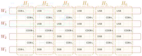
Figure 9. Understanding the meaning of width and height of our generator. In terms of feature dimension, our generator can be divided into 6 floors (denoted as H). The number of floors is the same as the height of our generator. For instance, $H_1$ means the 1th floor. In terms of the number of the information up and down stream, we can divide the generator into 4 streams (denoted as W). Each stream W combines a number of either USBs or DSBs.

In Figure 4a, every block on the same floor (height) releases the same shape of feature map by padding, represented by the same color of arrows. Before network processing begins in earnest, the input image goes through the shallow convolutional layer (kernel size = 3, stride = 1). Similarly, before it predicts the confidence map, the last feature map goes through a shallow convolutional layer, too. The former works the channel-expanding module and decides the capacity of information flow all through the network. Contrarily, the latter fuses information from the last feature map and makes a final decision (i.e., a prediction).

Each time it passes through the DSB, the feature map’s depth is doubled and the width and height are each halved. Conversely, passing through the USB, the depth of the feature map is cut in half, and the width and height are doubled. The ratio for the CDDB-L is calculated with Equation (11). Note that the units for the CDDB-L ratio is columns.

$$\begin{array}{c}\hfill \begin{array}{c}\hfill \mathrm{The}\mathrm{number}\mathrm{of}\mathit{CDDB}\text{-}\mathit{L}columns=(\mathit{width}-1)//3\end{array}\end{array}$$

(11)

The selective strategies are resizing (RS), shuffle (SF). Resizing is shown in Figure 10, and shuffle is shown in Figure 11. In resizing, we take the route for case 3. Each route in resizing does not show a dramatic performance gap, but the shuffle strategy is not the same. We cautiously adopted the direct through shuffle strategy as the end process within every CDB-L, and CDDB-L because of the validity of our sub-network, as explained in Section 3.2.2.

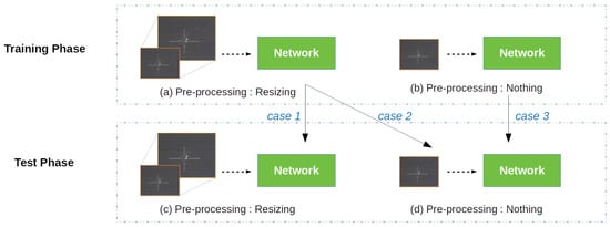
Figure 10. Each phase can choose to resize the input image or not. Asymmetric Contextual Modulation (ACM) [31] takes the route for case 1, since it exploits the backbone, and is constructed for large-scale object images. On the other hand, AVILNet takes the route for case 3, because it is constructed for small-object images from beginning to end.

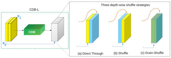
Figure 11. Shuffle strategies for last-fusion include (a) direct through, (b) shuffle, and (c) grain-shuffle. (b) and (c) differentiate our ensemble assistant network. Therefore, those strategies lead to the pool performance shown in Table 1.

The exact configurations of each block in the generator are shown in Table 5 and the input/output dimensions are shown in Table 6.

Table 5. Block details for CDB-L, CDDB-L, USB, and DSB. The growth rate and the number of dense layers for the CDB-L and CDDB-L are $\mathrm{gw}=24$ and $\mathrm{nd}=7$, respectively.

Block	Layer/Operation	Kernel/Dilation/Stride/Padding
CDB-L	conv-batch normalization-mish activation-concat conv-batch normalization-mish activation-concat conv-batch normalization-mish activation-concat conv-batch normalization-mish activation-concat conv-batch normalization-mish activation-concat conv-batch normalization-mish activation-concat conv-batch normalization-mish activation-concat conv-concat	$3\times 3,1,1,1$ $3\times 3,1,1,1$ $3\times 3,1,1,1$ $3\times 3,1,1,1$ $3\times 3,1,1,1$ $3\times 3,1,1,1$ $3\times 3,1,1,1$ $1\times 1,1,1,0$
CDDB-L	conv-batch normalization-mish activation-concat conv-batch normalization-mish activation-concat conv-batch normalization-mish activation-concat conv-batch normalization-mish activation-concat conv-batch normalization-mish activation-concat conv-batch normalization-mish activation-concat conv-batch normalization-mish activation-concat conv-concat	$3\times 3,1,1,1$ $3\times 3,2,1,2$ $3\times 3,4,1,4$ $3\times 3,8,1,8$ $3\times 3,16,1,16$ $3\times 3,32,1,32$ $3\times 3,64,1,64$ $1\times 1,1,1,0$
USB	transposed conv-batch normalization-mish activation conv-batch normalization-mish activation	$3\times 3,1,2,1$ $3\times 3,1,1,1$
DSB	conv-batch normalization-mish activation conv-batch normalization-mish activation	$3\times 3,1,2,1$ $3\times 3,1,1,1$

Table 6. Input and output dimensions for each block.

Block	Height	Input Dimension	Output Dimension
CDB-L, CDDB-L	1 2 3 4 5 6	128, 128, 34 64, 64, 68 32, 32, 136 16, 16, 272 8, 8, 544 4, 4, 1088	128, 128, 34 64, 64, 68 32, 32, 136 16, 16, 272 8, 8, 544 4, 4, 1088
USB	2 3 4 5 6	64, 64, 68 32, 32, 136 16, 16, 272 8, 8, 544 4, 4, 1088	128, 128, 34 64, 64, 68 32, 32, 136 16, 16, 272 8, 8, 544
DSB	2 3 4 5 6	128, 128, 34 64, 64, 68 32, 32, 136 16, 16, 272 8, 8, 544	64, 64, 68 32, 32, 136 16, 16, 272 8, 8, 544 4, 4, 1088

3.4.2. Discriminator

Our discriminator was motivated by U-GAT-IT [60], which exploits spectral normalization [61] to stabilize the training of the discriminator. Likewise, we applied spectral normalization to the end of each fully connected layer within the discriminator. The one average-pooling layer and the one max-pooling layer are settled at the front of each fully connected layer to escape the input-size dependency. This is a decisive difference, compared with DataLossGAN [22]. The whole structure of DataLossGAN is illustrated in Figure 2. As a result that there is no apparatus for compressing the feature map, DataLossGAN is dependent on the input-size. The whole structures of our discriminator are illustrated in Figure 4b. The specific configurations and the input/output dimensions of the discriminator are shown in Table 7.

Table 7. Details for our discriminator.

Input Dimension	Output Dimension	Layer/Operation	Kernel/Dilation/Stride/Padding
128, 128, 2 64, 64, 24 32, 32, 48 16, 16, 192	64, 64, 24 32, 32, 48 16, 16, 192 8, 8, 768	conv-batch normalization-lrelu activation conv-batch normalization-lrelu activation conv-batch normalization-lrelu activation conv-batch normalization-lrelu activation	4, 1, 2, 1 4, 1, 2, 1 4, 1, 2, 1 4, 1, 2, 1
8, 8, 768	1, 1, 2	avgpooling-fully connected layer-spectral normalization	$768\times 2$
8, 8, 768	1, 1, 2	maxpooling-fully connected layer-spectral normalization	$768\times 2$
1, 1, 4	2	addition-softmax	-

4. Experimental Results

In this section, we compare AVILNet with other related state-of-the-art ISOS methods and one small-object detection method, (YoloV4 [23]). In addition, plentiful results from the ablation study prove our approach is reasonable.

4.1. Methods in Comparison

We compared AVILNet with two groups: CNNs and handcraft-based methods. In the CNN group, two networks were not originally designed for the ISOS task. DeepLabV3 [48] is a generic large-object segmentation method, and YoloV4 [55] is a detector following the single-stage, one-shot affiliation method. They are based on the CNN, but are not designed for ISOS. Nevertheless, they are SOTA in their own fields. To obtain extensive discernment, they were included in CNN group. The other methods, DataLossGAN [22] and ACM [31], were designed for ISOS from beginning to end, and they achieved incredible performance on their datasets. For a non-partisan comparison, all methods were measured on the ICCV 2019 ISOS Single dataset only. The other group (handcraft-based) consisted of IPI [6], MPCM [32], PSTNN [37], MoG [62], RIPT [36], FKRW [33], NRAM [38], AAGD [34], Top-hat [13], NIPPS [35], LSM [19], and Max-median [21].

4.2. Hardware/Software Configuration

The experiment was conducted on a single GPU (RTX 3090) with a 3.4 GHz four-core CPU. All the handcraft-based methods were implemented in Python or Matlab and all the CNN-based methods were implemented in Pytorch. All weights within the networks underwent initialization [63], and all models were trained from scratch. For a fair competition, we singled out the best results from among all epochs for every method. Each method had the maximum number of epochs set to 130. Overall detailed settings of all methods are shown in Table 8.

Table 8. Detailed hyper-parameter settings of all the methods.

Methods	Parameter Settings
AVILNet	$bs=12,st=34,gw=24,nd=7,w=4,h=6,$ ${\lambda }_1=100,{\lambda }_2=10,{\alpha }_{1,2,3}=1,10,100,l{r}_{G,D}={10}^{-4},{10}^{-5}$, Adam optimizer
DataLossGAN	$bs=36,{\lambda }_1=100,{\lambda }_2=10,{\alpha }_{1,2}=100,10,l{r}_{G1,G2,D}={10}^{-4},{10}^{-4},{10}^{-5}$, Adom optimizer
ACM	$bs=260,lr=0.05,Resizingsize=480,\mathrm{number}\mathrm{of}\mathrm{block}=5$, Adagrad optimizer
YoloV4	$bs=4,lr=0.00261,Resizingsize=608$, Adam optimizer
DeepLabV3	$bs=25,lr={10}^{-4},Resizingsize=256$, SGD optimizer
IPI	Patch size = $50\times 50$, sliding step = 10, $\lambda =1/\sqrt{\min (\mathrm{m},\mathrm{n})}$, $ϵ={10}^{-7}$
MPCM	L = 3, N = 3, 5, 7, 9
PSTNN	Patch size = $40\times 40$, sliding step = 40, $\lambda =0.7/\sqrt{\max ({\mathrm{n}}_1,{\mathrm{n}}_2)\times {\mathrm{n}}_3}$, $ϵ={10}^{-3}$
MoG	Temporal sliding length = 3, Patch size = $50\times 50$, sliding step = 5, patch length = 3, $k=3$, $ϵ={10}^{-3}$
RIPT	Patch size = $16\times 16$, sliding step = 8, ${\lambda }_L=0.7$, $\mu =5$, $h=1$, $ϵ={10}^{-7}$
FKRW	Patch size = $11\times 11$, $k=4$, $p=6$, $\beta =200$
NRAM	Patch size = $50\times 50$, sliding step = 10, $\lambda =1/\sqrt{\min (\mathrm{m},\mathrm{n})}$, ${\mu }^0=3\times \sqrt{\max (\mathrm{m},\mathrm{n})}$, $\beta =3/\sqrt{\min (\mathrm{m},\mathrm{n})}$, $\gamma =0.002$, $C=\sqrt{\min (\mathrm{m},\mathrm{n})}/2.5$, $ϵ={10}^{-7}$
AAGD	K = 4, $\mathsf{\Phi }=\left[1,2,2,3\right]$, $\mathsf{\Omega }=\left[10,25,35,45\right]$
Top-hat	Patch size = $3\times 3$
NIPPS	Patch size = $50\times 50$, sliding step = 10, $\lambda =2/\sqrt{\min (\mathrm{m},\mathrm{n})}$, $ϵ={10}^{-7}$
LSM	L = 3, N = 3, 5, 7, 9
Max-median	$\mathrm{Patch}{\mathrm{size}}_{mean,median}=3\times 3$

4.3. Datasets

Wang, Huan et al. [22] published the ICCV 2019 ISOS Datasets consisting of two parts: AllSeqs and Single. The Single dataset contains 100 real, exclusive infrared images with different small objects, and AllSeqs contains 11 real infrared sequences with 2098 frames. The published version of the datasets is slightly different. The Single dataset remains unchanged, but AllSeqs is not provided as raw images, but as 10,000 synthetic augmented frames. The synthetic augmented frames consist of $128\times 128$ image patches which are randomly sampled from the raw images. This corresponds to configuration I in [22]. Accordingly, we conducted experiments under configuration I, in which, AllSeq was used for training and Single was used for test. Some Single examples are shown in Figure 1. All the training samples in AllSeqs have a size of $128\times 128$. To increase the difficulty of the tasks and ensuring an accurate evaluation of generalization capability, the backgrounds in the test images are not seen in the training images [22]. The detailed description about the ISOS datasets is given in Table 9.

Table 9. ISOS datasets: Nos. 1–11 are the eleven sequences in “AllSeqs”, dataset, and No. 12 is the single frame image dataset “Single”.

No.	Name	Size	Frames/Images
1	Canonball	$352\times 288$	30
2	Car	$344\times 256$	116
3	Plane	$320\times 240$	298
4	Bird	$640\times 480$	232
5	Cat	$216\times 256$	292
6	Rockets	$320\times 240$	242
7	Drone	$384\times 288$	396
8	Target1	$480\times 360$	361
9	Target2	$256\times 200$	30
10	Target3	$352\times 240$	50
11	Target4	$384\times 288$	51
12	Single-frame image set	Min: $173\times 98$, Max: $407\times 305$	100

4.4. Evaluation Metrics

In a CNN-based ISOS method, each binary pixel value indicates confidence in the object’s existence. Following [22], we set the threshold value at 0.5 to make a binary confidence map in all methods. In short, pixels with a score of less than 0.5, were ignored. In that state, precision–recall, the receiver operating characteristic, and F1-score were obtained by increasing the threshold value by 0.1. Finally, this measured data were used to obtain the average precision and area under the ROC curve, with the new F-area metric added to weigh the capability of real applications. Precision, recall, true positive rate (TPR), false positive rate (FPR) are calculated using Equation (12)

$$Precision=\frac{TP}{TP+FP}Recall=TPR=\frac{TP}{TP+FN}FPR=\frac{FP}{FP+TN}$$

(12)

$TP,FP,TN,$ and $FN$ stand for $TruePositive,FalsePositive,TrueNegative,$ and $FalseNegative$. $F1$-$score$ is calculated using Equation (13)

$$F1\text{-}score=2\times \frac{Precision\times Recall}{Precision+Recall}$$

(13)

4.5. New Metric: F-Area

$F1$-$score$ is used to measure harmonious performance. This is valuable for real applications, since the threshold value must be fixed when they operate. While operating with a fixed threshold value, the methods cannot educe full potential performance (i.e., average precision). To consider two cases simultaneously, we introduce a new metric: F-area. This metric takes into account both harmonious and potential performance aspects of any technique. F-area is simply obtained as the product of two values, expressed as:

$$\begin{array}{c}\hfill \begin{array}{c}\hfill F\text{-}area=AveragePrecision\times F1\text{-}score\end{array}\end{array}$$

(14)

5. Results and Discussion

5.1. Comparison with State-of-the-Art Methods

Evaluations of the performance by all other state-of-the-art methods are reported in Table 4 and are illustrated in Figure 12. In addition, some output results (denoted as a to e) are shown in Figure 13 and Figure 14. Our proposed AVILNet outperformed all the existing CNN-based and handcraft-based ISOS methods and detectors (i.e., YoloV4) in terms of all metrics. From the results of over-parameterization, AVILNet converges to a global minimum within just two epochs—overwhelmingly fewer iterations than the other methods (refer to Figure 15). On the other hand, ACM-FPN [31] recorded the second-best performance, despite having the fewest parameters and the minimum computing cost, although it recorded the highest number of iterations (91 epochs). That is an inevitable consequence based on the trade-off. In particular, DeepLab V3 [48] recorded the worst performance from among the CNN-based methods. Since DeepLab V3 was designed for large-scale objects, it is hard to forward small-object information to deep semantic layers. In addition, Yolo V4 was designed for large-scale objects, too. Nevertheless, how did it obtain such a fine performance? The answer to this question is that the backbone of Yolo V4 is based on the cross-stage partial network. CSP tends to forward information well into the deep semantic layers. AVILNet also exploits CSP to surmount the vanishing information problem. Meanwhile, all the handcraft-based methods obtained immature performance. These phenomena come from the overwhelming lack of filters to distinguish objects from the background, compared to the CNN-based methods.

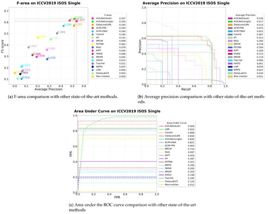
Figure 12. The performance of all state-of-the-art methods on the ICCV2019 ISOS Single dataset: (a) the proposed metric (F-area), (b) average precision, and (c) area under the ROC curve.

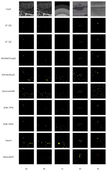
Figure 13. The results of CNN-based methods. Green, red, and yellow indicate true positive, false negative, and false positive, respectively. To make a binary map, a threshold value of 0.5 was applied for each method’s confidence map. GT(D) and GT(S) indicate ground truth for detection and segmentation, respectively.

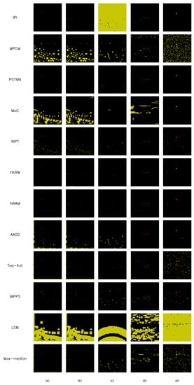
Figure 14. The results of handcraft-based methods.

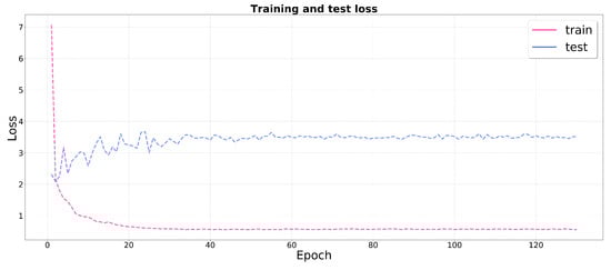
Figure 15. Training and test loss graphs for our AVILNet.

5.2. Ablation Study

In this section, we explore the following questions to ensure that the contributions of our proposed model components are reasonable. Then we answer the all questions point by point.

Question 1. Does thin pathway really block information flow?

Question 2. In ISOS, is resizing the input image instructive?

Question 3. Does ${\mathcal{L}}_2$ stabilize the regularization from over-parameterization?

Question 4. Height vs. width. What is more important?

Question 5. Are there just more dilation layers for better performance?

Question 6. How effective is the cross-stage partial strategy?

Question 7. What is the best shuffle strategy in last-fusion?

Question 8. Feature addition vs. attention-based feature addition. What is the best?

Question 9. Is the ratio of ${\lambda }_{MD,FA}$ suitable for our task?

Question 10. Is mish activation better than leaky ReLU activation in our task?

Question 11. Is the learning rate we used the best?

Question 12. Is the dual-learning system superior than the single in our case?

All hyper-parameters and selective strategies, except for the discriminator, were changed variously for the ablation study. We performed the massive experiments and divided them into four branches by subject. One is single (denoted as D), another is dual (denoted as T), a third is MEN, and the other (denoted as Q) is a step-by-step approach. Therefore, our plenty of experiments gave us considerable insight into finding the best way as shown in Table 1 and Table 10, and especially, Table 2, which clearly confirm the effectiveness of each contribution, step by step. Specifically, Table 1 is the experiments for the single network, Table 10 is for the dual networks, Table 3 is for the MEN, and Table 2 is for the step-by-step approach. The notations ${\mathrm{D}}_{index}$, ${\mathrm{T}}_{index}$, and ${\mathrm{Q}}_{index}$ indicate the corresponding relevant Table 1, Table 2, and Table 10, respectively. Especially, Table 2 clearly shows the effectiveness of each sectional idea, from the baseline to the proposed method. In this section, we skip the expression to indicate each table, and instead, we directly designate each index (e.g., D1, T1, Q1, etc.). All the graphical results for the each tables are shown in Figure 16, Figure 17 and Figure 18.

Table 10. Ablation study with diverse hyper-parameters and strategies for dual networks.

Index	gw	nd	w	h	RS	#	lr	$\mathit{L}2$	DL	L	${\mathit{\lambda }}_{\mathbf{MD}},{\mathit{\lambda }}_{\mathbf{FA}}$	ep	F1	AP	AUC	Fa
T1	4	3	3	1	3	64	${10}^{-3}$		✓		100, 10	5	0.577	0.491	0.847	0.283
	8	7	6	3	3	36	${10}^{-4}$		✓		100, 10
T2	4	3	3	1	1	64	${10}^{-4}$		✓		100, 1	4	0.532	0.384	0.741	0.204
	8	7	4	6	1	36	${10}^{-4}$		✓		1, 10
T3	4	3	3	1	3	64	${10}^{-3}$		✓	✓	100, 10	3	0.575	0.474	0.821	0.273
	8	7	6	3	3	36	${10}^{-4}$		✓	✓	100, 10
T4	16	4	2	4	3	16	${10}^{-4}$	✓		✓	100, 10	21	0.513	0.477	0.813	0.230
	16	4	3	6	3	16	${10}^{-4}$	✓		✓	100, 10
T5	4	3	2	3	3	64	${10}^{-4}$	✓	✓	✓	100, 10	5	0.530	0.447	0.805	0.237
	8	7	4	6	3	36	${10}^{-4}$	✓	✓	✓	100, 10
T6	4	3	2	3	3	64	${10}^{-4}$		✓	✓	100, 10	6	0.567	0.452	0.790	0.256
	8	7	4	6	3	36	${10}^{-4}$		✓	✓	100, 10
T7	24	7	4	6	3	34	${10}^{-4}$		✓	✓	100, 1	1	0.582	0.502	0.942	0.292
	24	7	4	6	3	34	${10}^{-4}$		✓	✓	100, 10
T8	24	7	4	6	3	34	${10}^{-4}$	✓	✓	✓	100, 1	1	0.610	0.536	0.928	0.327
	24	7	4	6	3	34	${10}^{-4}$	✓	✓	✓	100, 10

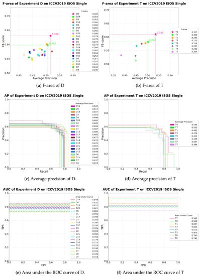
Figure 16. The performance of ablation study D and T.

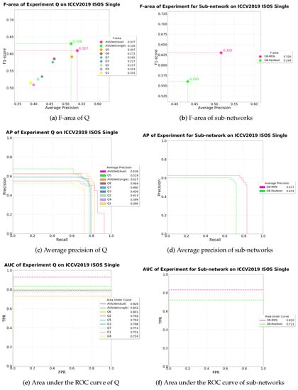
Figure 17. The performance of ablation study Q and sub-networks.

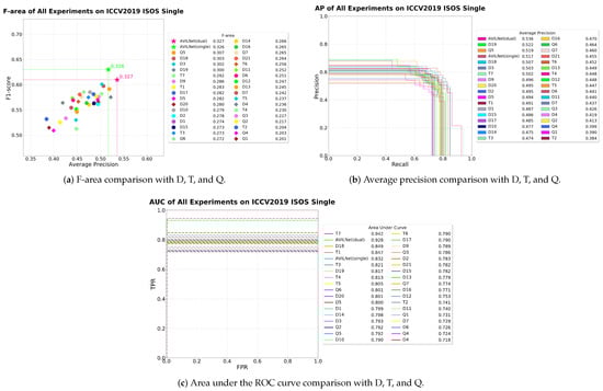
Figure 18. The performance of all ablation studies.

5.2.1. Question 1. Thin Pathway Blocks Information Flow

D1 has the thickness of a stream at 8, recording the best performance after 123 epochs. This slowest convergence-time result stems from the fact that this thin pathway blocks information flow. Likewise, T4 has a stream thickness of 16, recording the best performance after 21 epochs. It is the slowest convergence-time in group T (Table 10). To sum up, a pathway that is too narrow, compared to the amount of information within each block, not only creates a gradient bottleneck, but also leads to pool performance.

5.2.2. Question 2. In ISOS, Resizing the Input Image Is Adverse to the Performance

To confirm the effectiveness of the resizing strategy, we compared D2 with D3, and D17, and D18 with D8. D2 and D20 follow the route for case 1, and D19 follows the route for case 2 (see Figure 10). At first, for the training phase, resizing the input image is not beneficial. Then, for the test phase, resizing the test image is really deleterious. The route for case 1 reduces the performance of F-area (Fa) by up to 14%. The route for case 2 reduces it by 7.9%.

5.2.3. Question 3. ${\mathcal{L}}_2$ Slightly Stabilizes Regularization from Over-parameterization

$L_2$ is shown to be ambiguous in our case. We observed an anticipated phenomenon. This loss function consistently reduces performance on the subsets: (D3, D4), (T5, T6). However, subsets (D8, D21), and (T7, T8) show the opposite results. This is because of the difference in the number of parameters. The former have fewer trainable parameters than the latter. D3 and T5 have $62.08M$ and $76.92M$ parameters, respectively, while D8 and T7 have $80.98M$ and $161.96M$ parameters, respectively.

5.2.4. Question 4. Height Is More Important Than Width

The important decision in GridNet [24] is setting the ratio of the height to width of the network. The height mostly affects the maximum receptive field; contrarily, width affects the maximum stacked layer of each floor. To confirm if height or width is more important, we conducted experiments D5 and D11. In D5, we replaced the height with the width of D3. As a result, D5 had better pool performance than D3. Additionally in D11, to observe the effectiveness of the receptive field, we reduced the height of D8 by half, which reduced the performance by 22.7%. In conclusion, the height has to be longer than width of the network.

5.2.5. Question 5. Only the Proper Ratio of CDB-L to CDDB-L Can Improve the Performance

DataLossGAN [22] obtained successful performance by adopting a dilation layer [48]. Motivated by this success, we applied dilation layers in AVILNet. CDDB-L has dilation layers, as shown Figure 5. Then, how many CDDB-Ls are suitable? D6 and T1 exploit only CDDB-L. As a result, compared to D5, the performance of D6 decreased by 11%, but compared to T3, the performance of T1 increased by 3.5%. To concentrate on a single network study, we took the strategy following Equation (11).

5.2.6. Question 6. The Cross-Stage Partial Strategy Is Imperative to Overcome the Problem of Gradient Vanishing

One of the main contributions is applying CSP [25] in AVILNet. In ISOS, information vanishing from within a deep CNN is a significant issue [22,31]. To tackle this, we applied CSP to each dense block with last-fusion (denoted as CDB-L). This strategy alleviates the issue, and dramatically improved performance. To confirm our success, we conducted an experiment for D8 without CDBs (shown as D12). Compared to D8, the performance of D12 decreased by 24%. This result indicates that adopting CSP is essential.

5.2.7. Question 7. The Direct-through Shuffle Strategy Is Superior to the Other Strategies

In adopting CSP, we took the last-fusion strategy instead of the original for embedding the MEN described in Section 3.2.2. D9 and D10 selected shuffle, and grain-shuffle, respectively—the two strategies shown in Figure 11b,c. Compared to D8, denoted as AVILNet (Single), their performance decrease by 12% and 14%, respectively. These results underpin the superiority of our MEN.

5.2.8. Question 8. Attention-Based Feature Addition Is Better Than Simple Addition

Liu, Xiaohong et al. [45] proposed GridDehazeNet. This network replaced feature addition in GridNet [24] with attention-based feature addition. The difference between them is that the latter is able to use the weighted sum from trainable weights, as shown in Figure 19. D17 shows the significance of the weighted sum. When D17 took the simple addition strategy, it decreased by 13%, compared to D8. In our analysis, attention-based feature addition assumes a role discerning the information that is flowing on a grid-way. Therefore, this allows AVILNet to focus more on important information.

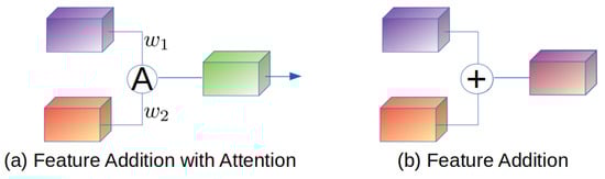
Figure 19. This figure illustrates the feature addition with attention and the feature addition. (a) Weighted sum of features. (b) Simple addition.

5.2.9. Question 9. The Ratio of ${\lambda }_{MD,FA}$ Is Dependent on Not only the Datasets but also the Network Configurations

Ratio ${\lambda }_{MD,FA}$ is needed for data loss [22]. In D15 and D16, we set ${\lambda }_{FA}$ at 3. This value is as low as 7, compared to D8. Therefore, they can concentrate more on reducing miss detections rather than false alarms. However, this attempt decrease performance by 16% and 18%, respectively. As a result, we followed the default ${\lambda }_{MD,FA}$ setting from [22]. Dual network T2 (which followed the setting in [22]) showed pool performance. Therefore, we set the ${\lambda }_{FA}$ at 1 for a dual network.

5.2.10. Question 10. Mish Activation Is Better Choice than Leaky ReLU

Misra et al. [64] proposed mish activation. This successfully surpasses the leaky ReLU (denoted as lrelu) [65]. We replaced lrelu with mish in AVILNet. Then, we observed performance increasing by 8.3%. This experiment is shown as D18.

5.2.11. Question 11. The Learning Rate at 0.0001 Is the Best

To adjust the learning rate, we conducted experiments D13, D14, and D18. Finally, we set the learning rate at ${10}^{-4}$. This is ten times smaller than the baseline’s learning rate.

5.2.12. Question 12. The Dual-Learning System Enhances the AP and AUC Well, but Increases the Fa Slightly

T8 consists of two D8 networks. The difference of T8 and D8 is only the ratio of ${\lambda }_{MD,FA}$. As D16 concentrates ${\lambda }_{MD}$ more than ${\lambda }_{FA}$ and T8 did not record the better performance, we can conclude that the dual-learning system has advantages over the single.

5.2.13. Applying the Experiment Step by Step

To see the effectiveness of each idea at a glance, we conducted the experiments denoted with Q. Additionally, we replaced all dense blocks [27] of our generator with Resnet [40] or ResNext [41] to ensure that the dense block [27] is the best choice. All results are shown in Table 2. Note that this sub-section is conducted to observe the effectiveness of each block. (Do not be confused by the sub-network experiment in Section 3.2.2, and Table 3) To improve the understanding about the problem of gradient vanishing, we have to notice the relationship between Q3 and Q4. Q4 has gw and nd at 34 and 7, respectively. While Q3 has gw and nd at 16 and 4. For Q4, The number of epoch for convergence decreases at 8 to 4. The whole performance deteriorates because Q4 encounters the gradient vanishing problem. Q5 shows that cross-stage partial strategy is sufficient to overcome the problem of gradient vanishing. Furthermore, we modified the original strategy of CSP to last-fusion so that our AVILNet (Single) achieved the best score. The experiments Q6 and Q7 are performed to confirm that any other blocks (e.g., Residual block and ResNext block) are valid. The results of them denote that dense block is superior to residual block and ResNext block in our task. Additionally, the result of Table 3 denotes our sub-network (MEN) is remarkable than ResNext.

6. Summary and Conclusions

In this paper, we proposed a novel network, AVILNet, to solve the infrared small-object segmentation problem. Motivated by the necessity for a flexible structure, we constructed the network based on GridNet [24]. Due to its amorphous characteristics, we could conduct various experiments to find the best optimal structure. This is a great benefit in terms of saving time to design the network. In addition, our multi-scale attention-based ensemble assistant network performed remarkably well when forwarding low-level information of small objects into the deep high-level semantic layers. It operates as an independent feature extractor within the network, and is derived from the last-fusion strategy. A plenty of ablation study and analysis underpins the logical validity of the structure in AVILNet. In addition, to measure performance, taking into account both the harmonious and the potential capability, we introduced a new metric: F-area. The advantage of F-area is striking on the infrared small-object segmentation. In the infrared small-object segmentation true negatives are greater than true positives overwhelmingly, therefore the receiver operating characteristic displays very high levels of score. Therefore, the comparison method using the receiver operating characteristic is meaningless than other evaluation metrics (e.g., average precision, F1-score). In this situation, our F-area can be a sensible evaluation metric. Finally the performance results demonstrate the superiority of AVILNet in terms of all metrics in the infrared small-object segmentation task.

References

- Teutsch, M.; Krüger, W. Classification of small boats in infrared images for maritime surveillance. In Proceedings of the 2010 International WaterSide Security Conference, Carrara, Italy, 3–5 November 2010; pp. 1–7. [Google Scholar] [CrossRef]
- Szpak, Z.L.; Tapamo, J.R. Maritime surveillance: Tracking ships inside a dynamic background using a fast level-set. Expert Syst. Appl. 2011, 38, 6669–6680. [Google Scholar] [CrossRef]
- Zhang, Y.; Li, Q.Z.; Zang, F.N. Ship detection for visual maritime surveillance from non-stationary platforms. Ocean. Eng. 2017, 141, 53–63. [Google Scholar] [CrossRef]
- Kim, S.; Lee, J. Scale invariant small target detection by optimizing signal-to-clutter ratio in heterogeneous background for infrared search and track. Pattern Recognit. 2012, 45, 393–406. [Google Scholar] [CrossRef]
- Deng, H.; Sun, X.; Liu, M.; Ye, C.; Zhou, X. Small infrared target detection based on weighted local difference measure. IEEE Trans. Geosci. Remote Sens. 2016, 54, 4204–4214. [Google Scholar] [CrossRef]
- Gao, C.; Meng, D.; Yang, Y.; Wang, Y.; Zhou, X.; Hauptmann, A.G. Infrared patch-image model for small target detection in a single image. IEEE Trans. Image Process. 2013, 22, 4996–5009. [Google Scholar] [CrossRef]
- Park, J.; Chen, J.; Cho, Y.K.; Kang, D.Y.; Son, B.J. CNN-based person detection using infrared images for night-time intrusion warning systems. Sensors 2020, 20, 34. [Google Scholar] [CrossRef]
- Yilmaz, A.; Shafique, K.; Shah, M. Target tracking in airborne forward looking infrared imagery. Image Vis. Comput. 2003, 21, 623–635. [Google Scholar] [CrossRef]
- Dong, X.; Huang, X.; Zheng, Y.; Bai, S.; Xu, W. A novel infrared small moving target detection method based on tracking interest points under complicated background. Infrared Phys. Technol. 2014, 65, 36–42. [Google Scholar] [CrossRef]
- Wang, X.; Ning, C.; Xu, L. Spatiotemporal difference-of-Gaussians filters for robust infrared small target tracking in various complex scenes. Appl. Opt. 2015, 54, 1573–1586. [Google Scholar] [CrossRef]
- Xiao, S.; Ma, Y.; Fan, F.; Huang, J.; Wu, M. Tracking small targets in infrared image sequences under complex environmental conditions. Infrared Phys. Technol. 2020, 104, 103102. [Google Scholar] [CrossRef]
- Dong, X.; Huang, X.; Zheng, Y.; Shen, L.; Bai, S. Infrared dim and small target detecting and tracking method inspired by human visual system. Infrared Phys. Technol. 2014, 62, 100–109. [Google Scholar] [CrossRef]
- Liu, T.; Li, X. Infrared small targets detection and tracking based on soft morphology Top-Hat and SPRT-PMHT. In Proceedings of the 2010 3rd International Congress on Image and Signal Processing, Yantai, China, 16–18 October 2010; Volume 2, pp. 968–972. [Google Scholar] [CrossRef]
- Bittner, L.; Heigl, N.; Petter, C.; Noisternig, M.; Griesser, U.; Bonn, G.; Huck, C. Near-infrared reflection spectroscopy (NIRS) as a successful tool for simultaneous identification and particle size determination of amoxicillin trihydrate. J. Pharm. Biomed. Anal. 2011, 54, 1059–1064. [Google Scholar] [CrossRef] [PubMed]
- Bellisola, G.; Sorio, C. Infrared spectroscopy and microscopy in cancer research and diagnosis. Am. J. Cancer Res. 2012, 2, 1. [Google Scholar] [PubMed]
- Kosaka, N.; Mitsunaga, M.; Longmire, M.R.; Choyke, P.L.; Kobayashi, H. Near infrared fluorescence-guided real-time endoscopic detection of peritoneal ovarian cancer nodules using intravenously injected indocyanine green. Int. J. Cancer 2011, 129, 1671–1677. [Google Scholar] [CrossRef]
- Zhang, R.; Huang, L.; Xia, W.; Zhang, B.; Qiu, B.; Gao, X. Multiple supervised residual network for osteosarcoma segmentation in CT images. Comput. Med. Imaging Graph. 2018, 63, 1–8. [Google Scholar] [CrossRef]
- Yu, Q.; Xie, L.; Wang, Y.; Zhou, Y.; Fishman, E.K.; Yuille, A.L. Recurrent saliency transformation network: Incorporating multi-stage visual cues for small organ segmentation. In Proceedings of the IEEE Conference on Computer Vision and Pattern Recognition, Salt Lake City, UT, USA, 18–23 June 2018; pp. 8280–8289. [Google Scholar] [CrossRef]
- Chen, C.L.P.; Li, H.; Wei, Y.; Xia, T.; Tang, Y.Y. A Local Contrast Method for Small Infrared Target Detection. IEEE Trans. Geosci. Remote Sens. 2014, 52, 574–581. [Google Scholar] [CrossRef]
- Tom, V.T.; Peli, T.; Leung, M.; Bondaryk, J.E. Morphology-based algorithm for point target detection in infrared backgrounds. In Signal and Data Processing of Small Targets 1993; International Society for Optics and Photonics: Orlando, FL, USA, 1993; Volume 1954, pp. 2–11. [Google Scholar] [CrossRef]
- Deshpande, S.D.; Er, M.H.; Venkateswarlu, R.; Chan, P. Max-mean and max-median filters for detection of small targets. In Signal and Data Processing of Small Targets 1999; International Society for Optics and Photonics: Denver, CO, USA, 1999; Volume 3809, pp. 74–83. [Google Scholar] [CrossRef]
- Wang, H.; Zhou, L.; Wang, L. Miss Detection vs. False Alarm: Adversarial Learning for Small Object Segmentation in Infrared Images. In Proceedings of the 2019 IEEE/CVF International Conference on Computer Vision (ICCV), Seoul, South Korea, 27 October–3 November 2019; pp. 8508–8517. [Google Scholar] [CrossRef]
- Bochkovskiy, A.; Wang, C.Y.; Liao, H.Y.M. YOLOv4: Optimal Speed and Accuracy of Object Detection. arXiv 2020, arXiv:2004.10934. [Google Scholar]
- Fourure, D.; Emonet, R.; Fromont, E.; Muselet, D.; Tremeau, A.; Wolf, C. Residual Conv-Deconv Grid Network for Semantic Segmentation. In Proceedings of the British Machine Vision Conference (BMVC), London, UK, 4–7 September 2017; Kim, T.-K., Stefanos Zafeiriou, G.B., Mikolajczyk, K., Eds.; BMVA Press: Norwich, UK, 2017; pp. 181.1–181.13. [Google Scholar] [CrossRef]
- Wang, C.Y.; Mark Liao, H.Y.; Wu, Y.H.; Chen, P.Y.; Hsieh, J.W.; Yeh, I.H. CSPNet: A new backbone that can enhance learning capability of cnn. In Proceedings of the IEEE/CVF Conference on Computer Vision and Pattern Recognition Workshops, Seattle, WA, USA, 16–18 June 2020; pp. 390–391. [Google Scholar] [CrossRef]
- Chen, L.C.; Papandreou, G.; Schroff, F.; Adam, H. Rethinking atrous convolution for semantic image segmentation. arXiv 2017, arXiv:1706.05587. [Google Scholar]
- Huang, G.; Liu, Z.; Van Der Maaten, L.; Weinberger, K.Q. Densely connected convolutional networks. In Proceedings of the IEEE Conference on Computer Vision and Pattern Recognition, Honolulu, HI, USA, 21–26 July 2017; pp. 4700–4708. [Google Scholar] [CrossRef]
- Long, J.; Shelhamer, E.; Darrell, T. Fully convolutional networks for semantic segmentation. In Proceedings of the IEEE Conference on Computer Vision and Pattern Recognition, Boston, MA, USA, 7–12 June 2015; pp. 3431–3440. [Google Scholar] [CrossRef]
- Ryu, J.; Kim, S. Small infrared target detection by data-driven proposal and deep learning-based classification. In Infrared Technology and Applications XLIV; International Society for Optics and Photonics: Orlando, FL, USA, 2018; Volume 10624, p. 106241J. [Google Scholar] [CrossRef]
- Zhao, D.; Zhou, H.; Rang, S.; Jia, X. An Adaptation of Cnn for Small Target Detection in the Infrared. In Proceedings of the IGARSS 2018—2018 IEEE International Geoscience and Remote Sensing Symposium, Valencia, Spain, 23–27 July 2018; pp. 669–672. [Google Scholar] [CrossRef]
- Dai, Y.; Wu, Y.; Zhou, F.; Barnard, K. Asymmetric Contextual Modulation for Infrared Small Target Detection. In Proceedings of the IEEE Winter Conference on Applications of Computer Vision—WACV 2021, Waikoloa, HI, USA, 5–9 January 2021. [Google Scholar]
- Wei, Y.; You, X.; li, H. Multiscale Patch-based Contrast Measure for Small Infrared Target Detection. Pattern Recognit. 2016, 58. [Google Scholar] [CrossRef]
- Qin, Y.; Bruzzone, L.; Gao, C.; Li, B. Infrared Small Target Detection Based on Facet Kernel and Random Walker. IEEE Trans. Geosci. Remote Sens. 2019, 57, 7104–7118. [Google Scholar] [CrossRef]
- Moradi, S.; Moallem, P.; Sabahi, M.F. A false-alarm aware methodology to develop robust and efficient multi-scale infrared small target detection algorithm. Infrared Phys. Technol. 2018, 89, 387–397. [Google Scholar] [CrossRef]
- Dai, Y.; Wu, Y.; Song, Y.; Guo, J. Non-negative infrared patch-image model: Robust target-background separation via partial sum minimization of singular values. Infrared Phys. Technol. 2017, 81, 182–194. [Google Scholar] [CrossRef]
- Dai, Y.; Wu, Y. Reweighted infrared patch-tensor model with both nonlocal and local priors for single-frame small target detection. IEEE J. Sel. Top. Appl. Earth Obs. Remote Sens. 2017, 10, 3752–3767. [Google Scholar] [CrossRef]
- Zhang, L.; Peng, Z. Infrared small target detection based on partial sum of the tensor nuclear norm. Remote Sens. 2019, 11, 382. [Google Scholar] [CrossRef]
- Zhang, L.; Peng, L.; Zhang, T.; Cao, S.; Peng, Z. Infrared small target detection via non-convex rank approximation minimization joint l2, 1 norm. Remote Sens. 2018, 10, 1821. [Google Scholar] [CrossRef]
- Srivastava, R.K.; Greff, K.; Schmidhuber, J. Training Very Deep Networks. In Proceedings of the Advances in Neural Information Processing Systems 2015 (NIPS 2015), Palais des Congrès de Montréal, Montréal, QC, Canada, 7–12 December 2015; Springer: Berlin/Heidelberg, Germany, 2015; pp. 2377–2385. [Google Scholar]
- He, K.; Zhang, X.; Ren, S.; Sun, J. Deep residual learning for image recognition. In Proceedings of the IEEE Conference on Computer Vision and Pattern Recognition, Las Vegas, NV, USA, 27–30 June 2016; pp. 770–778. [Google Scholar] [CrossRef]
- Xie, S.; Girshick, R.; Dollár, P.; Tu, Z.; He, K. Aggregated residual transformations for deep neural networks. In Proceedings of the IEEE Conference on Computer Vision and Pattern Recognition, Honolulu, HI, USA, 21–26 July 2017; pp. 1492–1500. [Google Scholar] [CrossRef]
- Huang, G.; Sun, Y.; Liu, Z.; Sedra, D.; Weinberger, K.Q. Deep networks with stochastic depth. In Proceedings of the European Conference on Computer Vision, Amsterdam, The Netherlands, 11–14 October 2016; pp. 646–661. [Google Scholar] [CrossRef]
- Szegedy, C.; Liu, W.; Jia, Y.; Sermanet, P.; Reed, S.; Anguelov, D.; Erhan, D.; Vanhoucke, V.; Rabinovich, A. Going deeper with convolutions. In Proceedings of the IEEE Conference on Computer Vision and Pattern Recognition, Boston, MA, USA, 8–12 June 2015; pp. 1–9. [Google Scholar] [CrossRef]
- Luong, M.T.; Pham, H.; Manning, C.D. Effective approaches to attention-based neural machine translation. arXiv 2015, arXiv:1508.04025. [Google Scholar]
- Liu, X.; Ma, Y.; Shi, Z.; Chen, J. Griddehazenet: Attention-based multi-scale network for image dehazing. In Proceedings of the IEEE International Conference on Computer Vision, Seoul, South Korea, 27 October–3 November 2019; pp. 7314–7323. [Google Scholar] [CrossRef]
- Araujo, A.; Norris, W.; Sim, J. Computing receptive fields of convolutional neural networks. Distill 2019, 4, e21. [Google Scholar] [CrossRef]
- Ronneberger, O.; Fischer, P.; Brox, T. U-net: Convolutional networks for biomedical image segmentation. In Proceedings of the International Conference on Medical Image Computing and Computer-Assisted Intervention, Munich, Germany, 5–9 October 2015; pp. 234–241. [Google Scholar] [CrossRef]
- Chen, L.C.; Zhu, Y.; Papandreou, G.; Schroff, F.; Adam, H. Encoder-decoder with atrous separable convolution for semantic image segmentation. In Proceedings of the European Conference on Computer Vision (ECCV), Munich, Germany, 5–9 October 2015; pp. 801–818. [Google Scholar] [CrossRef]
- Goodfellow, I.; Pouget-Abadie, J.; Mirza, M.; Xu, B.; Warde-Farley, D.; Ozair, S.; Courville, A.; Bengio, Y. Generative adversarial nets. In Proceedings of the Advances in Neural Information Processing Systems, Montreal, QC, Canada, 7–12 December 2014; pp. 2672–2680. [Google Scholar]
- Pathak, D.; Krahenbuhl, P.; Donahue, J.; Darrell, T.; Efros, A.A. Context encoders: Feature learning by inpainting. In Proceedings of the IEEE Conference on Computer Vision and Pattern Recognition, Las Vegas, NV, USA, 27–30 June 2016; pp. 2536–2544. [Google Scholar] [CrossRef]
- Karimpouli, S.; Tahmasebi, P. Segmentation of digital rock images using deep convolutional autoencoder networks. Comput. Geosci. 2019, 126, 142–150. [Google Scholar] [CrossRef]
- Isola, P.; Zhu, J.Y.; Zhou, T.; Efros, A.A. Image-to-image translation with conditional adversarial networks. In Proceedings of the IEEE Conference on Computer Vision and Pattern Recognition, Honolulu, HI, USA, 21–26 July 2017; pp. 1125–1134. [Google Scholar] [CrossRef]
- Wang, X.; Kong, T.; Shen, C.; Jiang, Y.; Li, L. Solo: Segmenting objects by locations. arXiv 2019, arXiv:1912.04488. [Google Scholar]
- Liu, W.; Anguelov, D.; Erhan, D.; Szegedy, C.; Reed, S.; Fu, C.Y.; Berg, A.C. Ssd: Single shot multibox detector. In Proceedings of the European Conference on Computer Vision, Amsterdam, The Netherlands, 11–14 October 2016; pp. 21–37. [Google Scholar] [CrossRef]
- Redmon, J.; Divvala, S.; Girshick, R.; Farhadi, A. You only look once: Unified, real-time object detection. In Proceedings of the IEEE Conference on Computer Vision and Pattern Recognition, Las Vegas, NV, USA, 27–30 June 2016; pp. 779–788. [Google Scholar] [CrossRef]
- Simonyan, K.; Zisserman, A. Very deep convolutional networks for large-scale image recognition. arXiv 2014, arXiv:1409.1556. [Google Scholar]
- Lin, T.Y.; Maire, M.; Belongie, S.; Bourdev, L.; Girshick, R.; Hays, J.; Perona, P.; Ramanan, D.; Zitnick, C.L.; Dollár, P. Microsoft COCO: Common Objects in Context. arXiv 2015, arXiv:1405.0312. [Google Scholar]
- Allen-Zhu, Z.; Li, Y.; Song, Z. A Convergence Theory for Deep Learning via Over-Parameterization. In Proceedings of the 36th International Conference on Machine Learning, Long Beach, CA, USA, 9–15 June 2019; Chaudhuri, K., Salakhutdinov, R., Eds.; Volume 97, pp. 242–252. [Google Scholar]
- Allen-Zhu, Z.; Li, Y.; Liang, Y. Learning and Generalization in Overparameterized Neural Networks, Going Beyond Two Layers. In Proceedings of the Advances in Neural Information Processing Systems, Vancouver, BC, Canada, 8–14 December 2019; Volume 32, pp. 6158–6169. [Google Scholar]
- Kim, J.; Kim, M.; Kang, H.; Lee, K.H. U-GAT-IT: Unsupervised Generative Attentional Networks with Adaptive Layer-Instance Normalization for Image-to-Image Translation. In Proceedings of the International Conference on Learning Representations, Addis Ababa, Ethiopia, 26 April–1 May 2020. [Google Scholar]
- Miyato, T.; Kataoka, T.; Koyama, M.; Yoshida, Y. Spectral Normalization for Generative Adversarial Networks. In Proceedings of the International Conference on Learning Representations, Vancouver, BC, Canada, 30 April–3 May 2018. [Google Scholar]
- Gao, C.; Wang, L.; Xiao, Y.; Zhao, Q.; Meng, D. Infrared small-dim target detection based on Markov random field guided noise modeling. Pattern Recognit. 2018, 76, 463–475. [Google Scholar] [CrossRef]
- He, K.; Zhang, X.; Ren, S.; Sun, J. Delving Deep into Rectifiers: Surpassing Human-Level Performance on ImageNet Classification. arXiv 2015, arXiv:1502.01852. [Google Scholar]
- Misra, D. Mish: A self regularized non-monotonic neural activation function. arXiv 2019, arXiv:1908.08681. [Google Scholar]
- Xu, B.; Wang, N.; Chen, T.; Li, M. Empirical Evaluation of Rectified Activations in Convolutional Network. arXiv 2015, arXiv:1505.00853. [Google Scholar]
Publisher’s Note: MDPI stays neutral with regard to jurisdictional claims in published maps and institutional affiliations. |
© 2021 by the authors. Licensee MDPI, Basel, Switzerland. This article is an open access article distributed under the terms and conditions of the Creative Commons Attribution (CC BY) license (http://creativecommons.org/licenses/by/4.0/).