An Improved Algorithm Robust to Illumination Variations for Reconstructing Point Cloud Models from Images

Abstract

Reconstructing 3D point cloud models from image sequences tends to be impacted by illumination variations and textureless cases in images, resulting in missing parts or uneven distribution of retrieved points. To improve the reconstructing completeness, this work proposes an enhanced similarity metric which is robust to illumination variations among images during the dense diffusions to push the seed-and-expand reconstructing scheme to a further extent. This metric integrates the zero-mean normalized cross-correlation coefficient of illumination and that of texture information which respectively weakens the influence of illumination variations and textureless cases. Incorporated with disparity gradient and confidence constraints, the candidate image features are diffused to their neighborhoods for dense 3D points recovering. We illustrate the two-phase results of multiple datasets and evaluate the robustness of proposed algorithm to illumination variations. Experiments show that ours recovers 10.0% more points, on average, than comparing methods in illumination varying scenarios and achieves better completeness with comparative accuracy.

1. Introduction

Three-dimensional reconstruction provides effective technical and data support for various applications through retrieving 3D information of real objects or scenes [1]. The corresponding innovations are evolving our life in several aspects, such as 3D movies, virtual reality, and heritage preservation [2,3]. Image-based reconstruction recovers 3D coordinate information from multiple visual images photographed at different viewpoints. It is a meaningful cross-discipline subject involving image processing, stereo vision, and computer graphics, which can generate realistic models and has broad application prospects on account of its flexibility and low cost [4,5].

Image-based reconstruction retrieves sparse or dense 3D point cloud of target objects or scenes. A sparse method extracts features matches from images and establish epipolar constraints to estimate and optimize camera parameters, and then recovers the structures of scenes from camera motions and feature matches. The recovered 3D point cloud is sparse and lacks scene details. To obtain dense point cloud model with richer details, a multi-view stereo scheme, seed-and-expand, is widely employed, which takes sparse seed feature matches as input and propagates them to the pixel neighborhoods, then restores the 3D points by stereo mapping using estimated camera parameters [6]. This scheme uses sparse features or points as seeds to build dense point cloud recursively and adaptively, such as PMVS [7] and VisualSfM [8]. However, the less distinctive pixels, such as those in the textureless regions, are not effectively processed due to inaccurate feature matching and imperfect constraints of diffusion, making the reconstructed results low in completeness [9]. At the same time, those methods are easily impacted by illumination, texture, or other photographic reasons, resulting in missing details or uneven distribution of retrieved points.

To address the mentioned issues to improve the completeness of retrieved point clouds, this paper proposes an enhanced reconstructing algorithm to push the seed-and-expand scheme to the furthest extent. The work has the following merits: (1) We propose an enhanced similarity metric for image-based 3D reconstruction algorithm to promote the quality of retrieved point clouds. The metric integrates the zero-mean normalized cross-correlation coefficient of illumination and that of texture information which are robust to illumination variations and textureless cases among images. (2) The proposed metric is defined straightforwardly and employed in the two-phase dense feature diffusion, combined with disparity gradient and confidence constraints, to improve the robustness of diffusion to get point cloud models rich details and reasonable distribution. (3) We conduct qualitative and quantitative tests and comparisons on multiple image datasets to evaluate the advantages of proposed algorithm in point density, running time, completeness, and accuracy, showing its robustness to illumination variations and textureless cases.

The rest of this work is organized as follows. Section 2 discusses the related work, and Section 3 outlines the main structure of the proposed pipeline. Section 4 prepares for followed dense diffusion. The details of proposed two-phase diffusion are presented in Section 5 and Section 6. Experimental evaluations and discussions are performed in Section 7. Then, Section 8 concludes this work.

2. Related Work

In the last few decades, reconstructing 3D point cloud models from images has gained sufficient research focus and achieved great improvements. A number of reconstruction methods with good robustness and accuracy have been developed, which could be classified into four categories.

2.1. Single Image-Based Methods

Single image-based methods retrieve the three-dimensional representations of objects or scenes by extracting the geometry information such as shape, texture, and positional relationship, combined with prior knowledge. This category mainly includes three sub-divisions: feature learning-, shape retrieval-, and geometric projection-based approaches. The feature learning-based approach [10] firstly establishes the database for image scenes and learns features for contained objects such as illumination, depth, texture, shape, etc. Then, it constructs probability functions for features of target objects and measures the similarities to the features in database. Lastly, it performs 3D reconstruction according to the database and gained similarities. This approach achieves high efficiency and is suitable for reconstruction of large-scale scenes or human bodies. However, the reconstructing results lie on a comprehensive database, which is a challenging issue in practice. The shape retrieval-based method [11,12] retrieves 3D shapes via analysis on captured image, known as Shape-from-X (SfX), in which X could be shade, silhouette, texture, occlusion, etc. In 2014, Chai et al. [13] proposed a Shape-from-Shading (SfS) based system to reconstruct high-quality hair depth map from a single portrait photo. This kind of method has high demands for illumination and image resolution; otherwise, the effectiveness is inferior. As the name suggests, geometric projection-based algorithm [14] uses geometric projection constraints (e.g., parallel lines or planes, perpendicular lines or planes, vanishing points, etc.) to calibrate cameras, and then predicts the depth of 3D geometry in a scene. Overall, this method only needs to preprocess the single image to obtain the 3D information of object. It can be executed efficiently. However, the reconstruction accuracy and reliability are unstable due to limited a priori knowledge or features.

2.2. Two Images-Based Methods

Two images-based methods recover the 3D information of scenes or objects by the parallax of spatial points in two views. The common way of reconstructing from two images is to build epipolar geometry constraints and then estimate the depth map by triangle measuring [15]. This could be implemented through the following steps: image capturing, camera calibration [16], feature extracting & matching [17], and 3D recovering. The recovering of 3D information can be done either by 3D mapping [18] or template-based machine learning. The reconstruction process of this category usually takes all pixels as features in the matching phase to obtain dense reconstruction, which is complicated and time-consuming, but still, reconstructing upon two images gains limited accuracy and integrity comparing to image sequence-based methods.

2.3. Image Sequence-Based Methods

Reconstruction based on the image sequence recovers the 3D structures of the real world from a series of images photographed around the target sequentially. This approach gains better detail and accuracy than other methods since more features and constraints of multi-view images are considered. Basically, this category could also be divided into three subdivisions [19].

2.3.1. Reconstruction Based on Depth Mapping

This approach merges the depth images derived from depth mapping to retrieve the complete 3D point cloud models of objects [20]. Bradley et al. [21] propose a method that matches the sub-pixels to get a depth map to ensure the precision of reconstruction. The team of Liu et al. [22] present a continuous depth estimation strategy for multi-view stereo. Similar depth map fusion using coordinate decent algorithm is developed by Li et al. [23]. The Bayesian reflection method [24,25] employs energy minimization constraints on multi-view depth images to get a complete depth surface. It needs an initial value to achieve the global optimization. Lasang et al. [26] propose a novel method that combines high resolution color and depth images for dense 3D reconstruction which can produce much denser and more all-over 3D results.

2.3.2. Reconstruction Based on Feature Propagation

This kind of algorithm extracts sparse point feature matches from input images and then tries to increase the number of correspondences in certain diffusion principles to generate a dense point cloud model. This is usually done by measuring the similarity of local regions in image pairs. “Optimal match firstly propagated [27]” spreads the matched features to their neighborhoods with respect to the spatial consistency in a greedy growing style. Later, a new approach [28] is presented to reconstruct the shape of an object or a scene from a set of calibrated images, which approximates the shape with a set of surfels and iteratively expands the recovered region by growing further surfels in the tangent direction. This technique does not rely on a prior shape or silhouette information for initialization. A propagation method based on Bayesian inference is proposed by Zhang and Shan [29]. It uses multiple matching points in an iterative propagation process, hence generating very dense 3D points with noise. Cech and Sara’s strategy [30] allows one-to-many pixel matches in the diffusion process. In 2014, Yang et al. [6] developed a Belief Propagation stereo matching algorithm which firstly utilizes the local stereo method to obtain an initial disparity map and then selects ground control points for global matching. A feature propagation approach can effectively increase the number of recovered points, but requires more processing time. Meanwhile, the accuracy relies on the accuracy of feature extracting and rationality of propagating constraints.

2.3.3. Patch-Based Reconstruction

Patch-based reconstruction firstly initializes 3D patches from retrieved points, and then reconstructs the surface of object or scene by patch propagation, where a patch means the quadrangle corresponds to a retrieved 3D point. Goesele et al. [31] proposed the first MVS method applied to Internet photo collections, which handles variation in image appearance. The stereo matching technique takes sparse 3D points reconstructed from structure-from-motion (SfM) as input and iteratively grows surfaces from these points. The Microsoft Live Lab and Snavely et al. jointly developed a photo tourism system [4,32] which is suitable for large-scale scenes, but weak on textureless regions. The team of Furukawa proposed a patch-based MVS method, known as PMVS [5,7]. Though the architecture of PMVS looks quite different from [31], the underlying ideas of them are strikingly similar. It initializes patches from retrieved sparse model points, and then recursively propagates seed patches to their neighborhoods to recover dense, accurate, and complete 3D point cloud models. PMVS maintains reconstruction information by 3D patches and the expanding and filtering operations are done globally by matching across all the available views. This causes severe scalability issues, which are later addressed in [33], known as CMVS, by clustering images into small collections. To improve the speed of reconstruction, Wu et. al. [9] implemented the seed-and-expand method on GPU and accelerated a lot. An interactive reconstruction pipeline [34] is developed for monocular mobile devices with real-time feedback, which uses available on-device inertial sensors to make resilient tracking and mapping for rapid motions and estimates the metric scale of captured scenes. Lasang [26] utilizes 3D patches from high resolution color images for high texture regions and depth map for low texture regions. It achieves good results, but the computation cost is high. Based on this research, several open-source software programs are developed, such as Bundler [35] and VisualSfM [8]. VisualSfM incorporates SfM and CMVS algorithms to implement 3D reconstruction, which is a highly optimized and integrated tool.

PMVS is considered as one of the best 3D reconstruction methods available, which does not need any prior knowledge but generates better results. Combined with SfM, the reconstruction for unordered image collections or large outdoor scenes can be easily realized. Despite these, there still are shortcomings in practical application. For objects with complex structures, smooth surfaces or textureless regions, there exists a loss of details or local holes in reconstructed models. For large scale scenes, the input images with varying illuminations will cause scattered point clouds.

2.4. Deep-Learning-Based Reconstruction

Since 2015, many deep-learning-based 3D reconstruction methods are presented, among which the point-based technique is simple but efficient in terms of memory requirements [36]. Similar to volumetric [37,38] and surface-based representations [39,40], point-based techniques follow the encoder–decoder model. In general, grid representations use up-convolutional networks to decode the latent variable [41,42]. Point set representations use fully connected layers [43,44,45] since point clouds are unordered. Fan et al. [46] proposed a generative deep network that combines both the point set representation and the grid representation. The network is composed of a cascade of encoder–decoder blocks. Tatarchenki et al. [47] and Lin et al. [48] followed the same idea, but their decoder regresses N grids. Point set representations require fixing in advance the number of points N, while, in methods that use grid representations, the number of points can vary based on the nature of the object, but it is always bounded by the grid resolution.

The success of deep learning techniques depends on the availability of training data; unfortunately, the size of the publicly available datasets that include both images and their 3D annotations is small compared to the training datasets used in tasks such as classification and recognition. In addition, deep-learning methods are primarily dedicated to the 3D reconstruction of generic objects in isolation, and current state-of-the-art techniques are only able to recover the coarse 3D structure of shapes. Prior knowledge of the shape class are required to improve the quality of reconstruction. These limitations make deep-learning-based methods not suitable for complex targets or cluttered outdoor scenes.

3. Framework of 3D Reconstruction

As discussed in Section 2, the factors of illumination, texture, and shooting condition bring challenges to the image-based 3D reconstruction. The seed-and-expand scheme takes sparse seed feature matches as input and diffuses them to the pixel neighborhoods to build dense point cloud, recursively. The pruning criteria and diffusion strategy for seed features are crucial to this scheme. A qualified metric should be robust to the differences in illumination or photographic noise, and be able to take into account the smooth or textureless cases.

In this paper, an enhanced two-phase dense diffusing method is proposed to reconstruct the point cloud models of real scenes or objects from captured image sequences. Different from the existing algorithms, the proposed method considers both the illumination and texture factors to define the diffusion criteria. It integrates the zero mean normalized cross-correlation coefficient of illumination and the normalized cross-correlation coefficient of texture as matching metric in both feature diffusion and patch diffusion to generate dense point cloud models. As Figure 1 illustrates, the scheme consists of three main stages.

• Preprocessing. The seed-and-expand dense reconstruction scheme takes sparse seed feature matches as input and propagates them to the neighborhoods, and then restores the 3D points by stereo mapping using calibrated camera parameters. This step calibrates the input images to yield camera parameters and extract features for subsequent feature matching and diffusion. It is the preparation stage of the whole algorithm.
• Feature diffusion. Initializes seed matches from extracted features employing image pruning and epipolar constraints. Then, it propagates them to the neighborhoods by the similarity metric of each potential match, combining the constraints of disparity gradient and confidence measure as filtering criteria. Afterwards, it elects the eligible ones and retrieves 3D points by triangulation principle. This stage generates comparative dense points for the following patch diffusion in 3D space.
• Patch based dense diffusion. 3D patch is firstly defined at each retrieved point. As similar in the feature diffusion stage, seed patches are pruned by the appearance consistency (the proposed similarity metric) and geometry consistency, and then expanded within the grid neighborhoods to gain dense patches. At last, the expanded patches are filtered. This stage is recursively proceeded in multiple rounds, and the final 3D point cloud is obtained from retained patches.

The details of each stage are described separately in the following three sections.

4. Preprocessing

4.1. Camera Parameter Estimation

The goal of image-based 3D reconstruction can be described as “given a set of photographs of an object or a scene, estimate the most likely 3D shape that explains those photographs [7]”, which is also known as multi-view stereo. It takes a set of images and the corresponding camera parameters (intrinsic and extrinsic parameters) as input to retrieve the potential 3D information. Owing to the success of the SfM algorithm, the camera parameters could be reasonably estimated. Since MVS algorithms are sensitive to the accuracy of the estimated camera parameters, the bundle adjustment [49] that minimizes the following root-mean-squared-error (Equation (1)) is a necessity to optimize the initial camera parameters. Here, $\mathcal{C}\left(j\right)$ is the list of camera indices where the 3D point ${\mathbf{M}}^j\in \mathcal{M}$ is visible, $P_i\left({\mathbf{M}}^j\right)$ denotes the projected 2D image coordinate of point ${\mathbf{M}}^j$ in the ith camera by the camera parameters $P_i\in \mathcal{P}$, and ${\mathbf{m}}_i^j$ indicates the actually observed image coordinate of point ${\mathbf{M}}^j$.

$$\xi (\mathcal{P},\mathcal{M})=\sqrt{\sum _{j=1}^N\sum _{i\in \mathcal{C}\left(j\right)}{|P_i\left({\mathbf{M}}^j\right)-{\mathbf{m}}_i^j|}^2}$$

(1)

4.2. Feature Extraction

In the MVS, solving for the 3D information of a scene by known camera parameters is equivalent to matching pixel correspondences across the input images, which is done by feature extraction. In this work, Harris [17] and DoG (Difference of Gaussian [50]) are applied on the input images to extract local features with various properties. Note that the following correspondence matching must be operated within the same features, the cross-matching between different features is unallowable.

5. Feature Diffusion

Feature points are the sparse representation of input images. If only the matched feature correspondences are used to reconstruct 3D scene, the reconstructed result is sparse and low in completeness. This section introduces the feature diffusion process to increase the number of correspondences for dense reconstruction.

5.1. Correspondence Initialization

Since that only the images captured in nearby viewpoints share the similar features, the input images require pruning to reduce the unnecessary attempts in feature diffusion. For each reference image, we investigate the intersection angles between its optical axis (obtained by SfM) and that of other images, only the ones with intersection angle smaller than $\theta$ are taken as candidate images. In practice, it is divided into three cases [5] according to the number n of input images (Equation (2)):

$$\left\{\begin{array}{cc}Nopruning,\hfill & \hfill n\le 15\\ \theta ={60}^{°},\hfill & \hfill 15<n<60\\ \theta =10\times {360}^{°}/n,\hfill & \hfill n\ge 60\end{array}\right.$$

(2)

The image pruning prompts the matching efficiency by avoiding numerous meaningless attempts, meanwhile, reserves enough potential matches. After that, feature correspondences are initialized. For each feature point $x_1$ in the reference image, find the corresponding feature point $x_2$ in the candidate image by the epipolar geometry constraint and match them as initial correspondence ($x_1$, $x_2$) which are then collected as seeds for diffusion.

5.2. Calculation of Similarity

Theoretically speaking, the geometric constraint unifies the appearance consistency, which implies that the two parts of a correspondence should share the same or similar appearance since they are the projections of the same 3D point. Otherwise, it cannot be selected as diffusing seed due to the low confidence. Therefore, it is crucial to define a rational metric to appraise the appearance consistency of the feature correspondence.

In this work, we propose an enhanced metric to weigh the appearance similarity of the potential correspondences for diffusion. This metric integrates the zero-mean normalized cross-correlation coefficient (ZNCC [27]) of illumination and that of texture information. The former weakens the influence of illumination variation, and the later deals with the textureless case. The combination of these two terms assures the robustness of this metric to different shooting conditions. The appearance similarity ${\psi }_{tz}$ of a feature correspondence ($x,x^{\prime }$) is defined by Equation (3). In addition, the value range of appearance similarity is [−1, 1], where the large value corresponds to high similarity:

$${\psi }_{tz}=\lambda {\psi }_z+(1-\lambda ){\psi }_t$$

(3)

In Equation (3), ${\psi }_z$ represents the ZNCC of illumination of correspondence ($x,x^{\prime }$) defined by Equation (4), where $L\left(i\right)$ denotes the illumination (the L component in $Lab$ color space) of pixel i in the window $W_x$ centered at x, and $\overline{L}\left(x\right)$ is the average illumination of pixels in this window. Different from NCC (normalized cross-correlation coefficient), ZNCC performs zero-centered operation on the pixel illumination before normalization. This operation assures that the similarity metric is determined by the relative disparity of pixel illumination to that of the center pixel in the neighbouring window. Hence, it is adaptive to strong illumination variations among images and can enhance the robustness of diffusion to shooting conditions. The range of ${\psi }_z$ is [−1, 1], and the higher ZNCC value means that the two feature points in images are more relevant.

$${\psi }_z(x,x^{\prime })=\frac{{\displaystyle \sum _{i\in W_x,j\in W_{x^{\prime }}}}(L\left(i\right)-\overline{L}\left(x\right))(L\left(j\right)-\overline{L}\left(x^{\prime }\right))}{\sqrt{{\displaystyle \sum _{i\in W_x}}{(L\left(i\right)-\overline{L}\left(x\right))}^2{\displaystyle \sum _{j\in W_{x^{\prime }}}}{(L\left(j\right)-\overline{L}\left(x^{\prime }\right))}^2}}.$$

(4)

${\psi }_t$ indicates the ZNCC of texture between two image windows respectively centered at x and $x^{\prime }$. It is derived from the gray value of the $rgb$ pixel (Equation (6)) to deal with the textureless case, and the range is [−1, 1]. The window regions with similar visual appearance corresponds to the large value of ${\psi }_t$, and this principle is beneficial to the diffusion in smooth region. In proposed metric, ${\psi }_t$ is determined by Equation (5) in which $I\left(i\right)$ and $\overline{I}\left(x\right)$ respectively labels the gray value of pixel i and the average gray value in a window centered at x:

$${\psi }_t(x,x^{\prime })=\frac{{\displaystyle \sum _{i\in W_x,j\in W_{x^{\prime }}}}(I\left(i\right)-\overline{I}\left(x\right))(I\left(j\right)-\overline{I}\left(x^{\prime }\right))}{\sqrt{{\displaystyle \sum _{i\in W_x}}{(I\left(i\right)-\overline{I}\left(x\right))}^2{\displaystyle \sum _{j\in W_{x^{\prime }}}}{(I\left(j\right)-\overline{I}\left(x^{\prime }\right))}^2}}$$

(5)

$$I\left(x\right)=0.299r+0.587g+0.114b$$

(6)

5.3. Correspondence Diffusion

After determining the similarity of feature matches, a rigorous screening process is performed to select the reliable seeds for subsequent dense diffusion. The feature matches are divided into three groups according to the value of ${\psi }_{tz}$. In the diffusions, we introduce five parameters <${\mu }_1,{\mu }_2,{\mu }_3,{\mu }_4,{\mu }_5$> to divide the matches to different groups in which they will be treated accordingly. These thresholds influence the accuracy of diffusion. Loose or restrict setting leads to dense or sparse point clouds:

-

Matches with ${\psi }_{tz}\ge {\mu }_1$ are not only selected as candidates for restoring 3D points, but also pushed into the seed queue for diffusion.

-

Matches with ${\mu }_2\le {\psi }_{tz}\le {\mu }_1$ are only reserved as candidates for 3D points restoring.

-

Matches with ${\psi }_{tz}\le {\mu }_2$ are treated as false correspondences and deleted from the set.

5.3.1. Diffusing

Propagate seed matches with ${\psi }_{tz}\ge {\mu }_1$ to their local neighborhoods. For each seed, build multi-to-multi matchings in the 3 × 3 pixel windows of its host images, as depicted in Figure 2. Take correspondence ($p_{11},q_{22}$), for instance, the propagation occurs in windows $W_l$ and $W_r$ where potential matches are generated between the pixels in these two neighboring windows.

Then, filter the propagated matches and retain the reliable ones. Since many false or one-to-multi matches are generated in the propagation process, further constraints are required to prune the ineligible ones. In this work, the constraints of disparity gradient and the confidence measure are employed.

Disparity gradient constraint implies that the disparity of two neighboring matches is small, which can be used to eliminate the ambiguous one-to-multi matches. As Equation (7) defines, for two neighboring feature matches ($u,u^{\prime }$) and ($x,x^{\prime }$) from the same reference and candidate images, the discrete 2D disparity gradient should be no more than a threshold $\epsilon$:

$$\left|\right|(u-u^{\prime })-(x-x^{\prime }){\left|\right|}_{\infty }\le \epsilon$$

(7)

Confidence measure based on image gray value is given in Equation (8). This constraint reveals that a pixel point is unqualified for further matching or growing if the difference of gray value between this pixel and its 4-neighbors hits a threshold $\rho$:

$$\begin{array}{c}\hfill s\left(x\right)=\max \left\{\right|I(x+\mathsf{\Delta }x)-I\left(x\right)\left|\right\}\le \rho \end{array}$$

(8)

5.3.2. Secondary Diffusing

To further densify the reconstruction, a secondary propagation process is performed on diffused matches that meet the mentioned constraints. Calculate the similarity metric for the new matches, then push the matches with ${\psi }_{tz}\ge {\mu }_3$ to seed the queue for next round of propagation and choose the matches with ${\psi }_{tz}\ge {\mu }_4$ (${\mu }_3>{\mu }_4$) for 3D candidates only, as previous operations. Since the propagated matches are diffused from the original feature matches, so in practice, the thresholds ${\mu }_3/{\mu }_4$ should be slightly larger than ${\mu }_1/{\mu }_2$ to obtain reliable propagation.

5.4. 3D Points Restoring

After getting dense candidate feature matches, the spatial 3D points are recovered from the diffused matches by the triangulation principle.

6. Patch-Based Dense Diffusion

This section further densifies the point cloud models by the patch-based diffusion which takes the recovered 3D points as input and diffuses them in 3D space to produce denser points. The patch densification includes the following steps.

6.1. Patch Initialization

The patch p is defined as a rectangle of normal $\mathbf{n}\left(p\right)$ centered at the 3D point $\mathbf{c}\left(p\right)$, as Figure 3 shows. $\mathbf{n}\left(p\right)$ denotes the unit vector from point $\mathbf{c}\left(p\right)$ to the optical center $\mathbf{O}\left(R\right)$ of the reference image. Here, the reference image $R\left(p\right)$ is chosen so that its retinal plane is parallel to p as much as possible. In turn, $R\left(p\right)$ determines the orientation and extent of the rectangle p so that the projection of one of its edges into $R\left(p\right)$ is parallel to the image rows and that the smallest axis-aligned square covers the $\alpha \times \alpha$ ($\alpha$ = 7) pixel${}^2$ area [33]. Two constraints are employed to select reliable seed patches: geometry consistency and appearance consistency.

Define ${\mathcal{V}}^{*}\left(p\right)$ the candidate visible images of patch p. Geometry consistency refers to that the intersection angle between $\mathbf{n}\left(p\right)$ and the vector from $\mathbf{c}\left(p\right)$ to the optical center of visible image $I_i$ is less than a threshold, as given in Equation (9) and illustrated in the upper-right part of Figure 3. Appearance consistency denotes that the similarity between the projection of p on the reference image and that on each visible image follows the criteria in Equation (10). $\mathcal{V}\left(p\right)$ represents the set of visible images that satisfy the appearance consistency:

$${\mathcal{V}}^{*}\left(p\right)=\left\{I_i|I_i\in \mathcal{I},\mathbf{n}\left(p\right)·\frac{\mathbf{O}\left(I_i\right)-\mathbf{c}\left(p\right)}{|\mathbf{O}\left(I_i\right)-\mathbf{c}\left(p\right)|}>cos\frac{\pi }{3}\right\}$$

(9)

$$\mathcal{V}\left(p\right)=\left\{I_i|I_i\in {\mathcal{V}}^{*}\left(p\right),{\psi }_{tz}\ge {\mu }_5=0.7\right\}$$

(10)

Construct patch $p=\left\{\mathbf{c}\right(p),\mathbf{n}(p),R(p),\mathcal{V}(p\left)\right\}$ for each retrieved 3D point and consider the number of its visible images. If $\left|\mathcal{V}\right(p\left)\right|\ge 3$, then put p into the set $\mathcal{P}$ of seed patches, meaning that the patch is more likely to be seen in images. Otherwise, patch p is not eligible for diffusion.

6.2. Patch Expansion

Patch expansion densifies the seed patches so that the model surface could be covered as much as possible. To achieve this goal, each image is associated with a regular grid of $\beta \times \beta$ ($\beta =2$) pixel${}^2$ cells, then the patches are diffused to its neighboring cells under the following constraints to assure uniform patch coverage. The seed patch is diffused when no similar patches can be observed in its neighboring cells, as case (b) in Figure 3 shows. Otherwise, if the patch in neighboring cell is close to or share high similarity value with the seed patch, then no patch propagation, as case (a) and case (c) reveal.

Pop one seed patch p from the queue $\mathcal{P}$, and then locate its host cell in visible image $I_i$ and determine the neighboring cells $\mathcal{G}$(p). Proceed the following procedures for each eligible cell in $\mathcal{G}$(p):

-

Generate a new patch $p^{\prime }$ by copying p, then optimize its center $\mathbf{c}\left(p^{\prime }\right)$ and normal $\mathbf{n}\left(p^{\prime }\right)$ by maximizing the similarity score;

-

Gather the visible images $\mathcal{V}$($p^{\prime }$). If $\left|\mathcal{V}\right(p^{\prime }\left)\right|\ge 3$, then push $p^{\prime }$ to $\mathcal{P}$.

Execute the above steps for each element in $\mathcal{P}$ until the queue is empty. Through this way, the patches are propagated to its neighbors.

6.3. Patch Filtering

Likewise, there are outlier patches generated in patch expansion, hence patch filtering is necessary. Here, we employ the visibility and geometry constraints similar to [33] to remove outliers. Firstly, consider a patch p and the set $\mathcal{U}$ it occludes. Remove p as an outlier if $\left|\mathcal{V}\left(p\right)\right|{\overline{\psi }}_{tz}\left(p\right)<{\sum }_{p_i\in \mathcal{U}}{\overline{\psi }}_{tz}\left(p_i\right)$. Intuitively, when p is an outlier, both $\mathcal{V}$(p) and ${\overline{\psi }}_{tz}\left(p\right)$ are expected to be small, and p is likely to be pruned. Secondly, for each patch p, collect the patches lying in its host and adjacent cells in all images of $\mathcal{V}$(p). A quadric surface is then fitted by each patch and its neighbors. The ones with obvious fitting residuals are filtered.

Iterate above expansion and pruning steps for three rounds, and then obtain the final dense point cloud model by gathering the center points of all reserved patches.

7. Experimental Evaluation

This section evaluates the proposed image sequence-based 3D reconstruction algorithm. We illustrate the two-phase results of multiple datasets and evaluate the robustness of the proposed algorithm to illumination variations and textureless cases by comparing with other methods. All the experiments are carried out in C++ programming language on the machine equipped with 2.4 GHz multi-core CPU and 8 GB memory. In our experiments, $\lambda$ is empirically set to 0.5, and other thresholds are: ${\mu }_1=0.8$, ${\mu }_2=0.6$, ${\mu }_3=0.85$, ${\mu }_4=0.65$, ${\mu }_5=0.7$, $\epsilon =1.0$, $\rho =2.25$.

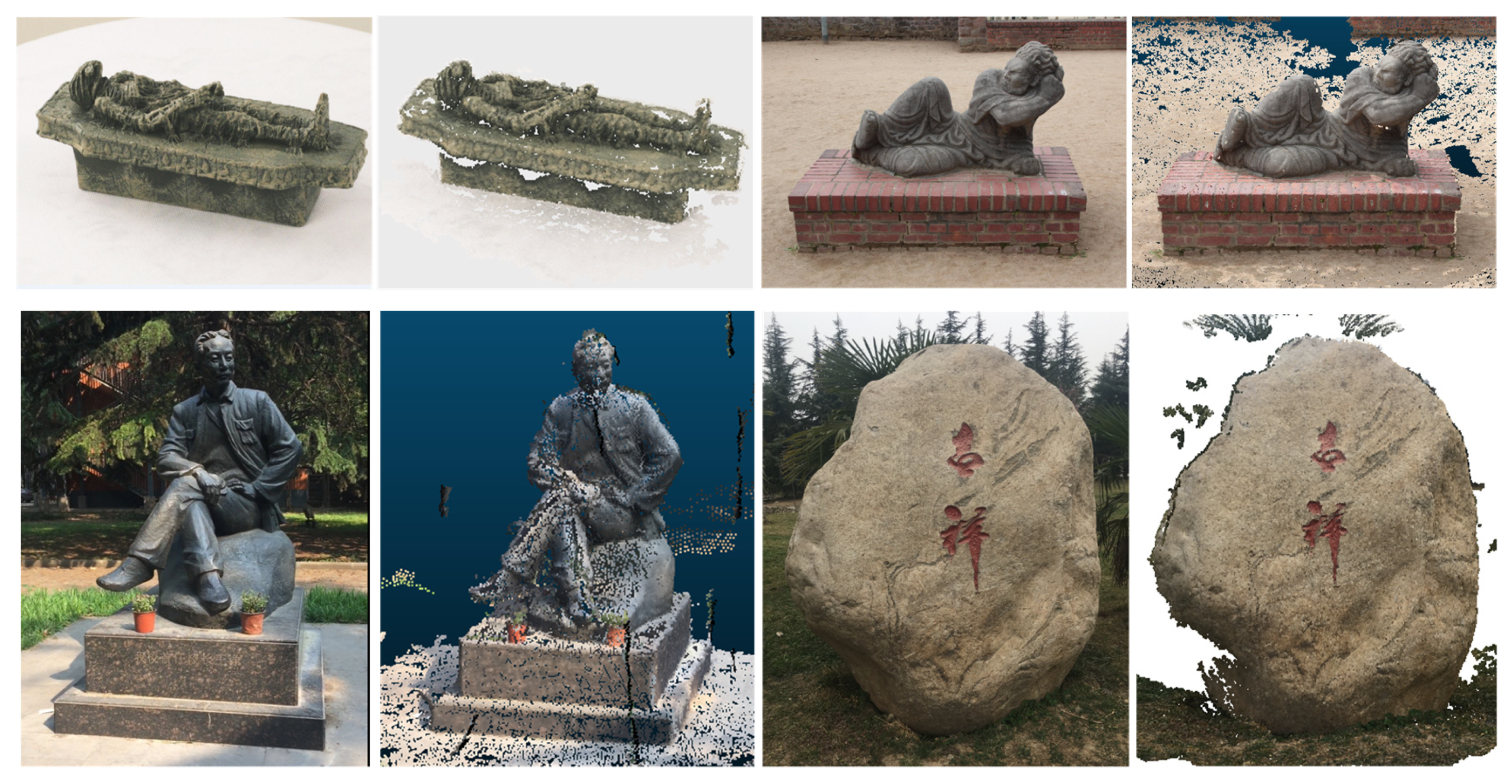
7.1. Reconstruction Results of the Proposed Method

The proposed reconstruction algorithm is experimentally evaluated on multiple datasets. The retrieved point clouds of three datasets via two phases of diffusion are illustrated in Figure 4. The middle columns and right column list the retrieved point clouds after feature diffusion and patch diffusion, respectively. It is observed that the feature diffusion phase constructs the basic structures of photographed models; however, the points are not dense and there are missing parts in the recovered point cloud models, such as the back and feet of “Dino16”, the stairs and pillars of “Temple16”, and the plain walls of “Fountain25”. The reason lies in that it is hard to extract and diffuse the feature matches in those areas. Starting from these results, patch diffusion recovers more 3D points to fill the missing parts to generate dense point clouds with rich details, which is valid for both smooth areas (e.g., back of “Dino16” and walls of “Fountain25”) and textured areas (e.g., feet of “Dino16”, stairs and pillars of “Temple16”). On average, patch diffusion increases the number of retrieved points by over 40% from feature diffusion (refer to the figures in

Table 1. Two phase results of the proposed algorithm on testing datasets.

Image Sequences			Retrieved Points
Name	No.	Resolution	Feature Diffusion	Patch Diffusion
Dino16	16	640 × 480	7329	8834
Dino48	48	640 × 480	6369	9694
Dino363	363	640 × 480	21,679	33,869
Temple16	16	480 × 640	5936	8458
Temple47	26	480 × 640	15,106	20720
Mummy24	24	1600 × 1100	36,384	48,272
Fountain25	25	3072 × 2048	355,330	463,935
Stone39	39	3024 × 4032	469,342	624,971
Sculpture58	58	2592 × 1728	600,217	997,770
Statue70	70	1920 × 1080	50,972	75,688

).

Generally speaking, more detailed and denser point clouds can be reconstructed from the dataset with more images. We compared the results from multiple image sequences of the same targets “Dino” and “Temple”. In addition, the figures in Table 1 draw the conclusion that a larger dataset produces a denser point cloud model. In addition, we applied the proposed algorithm on the other four datasets with different capacities or resolutions, and the recovered point clouds are demonstrated in Figure 5. Experimental results reveal that the proposed method is able to output dense and reasonable 3D point cloud models for different image sequences.

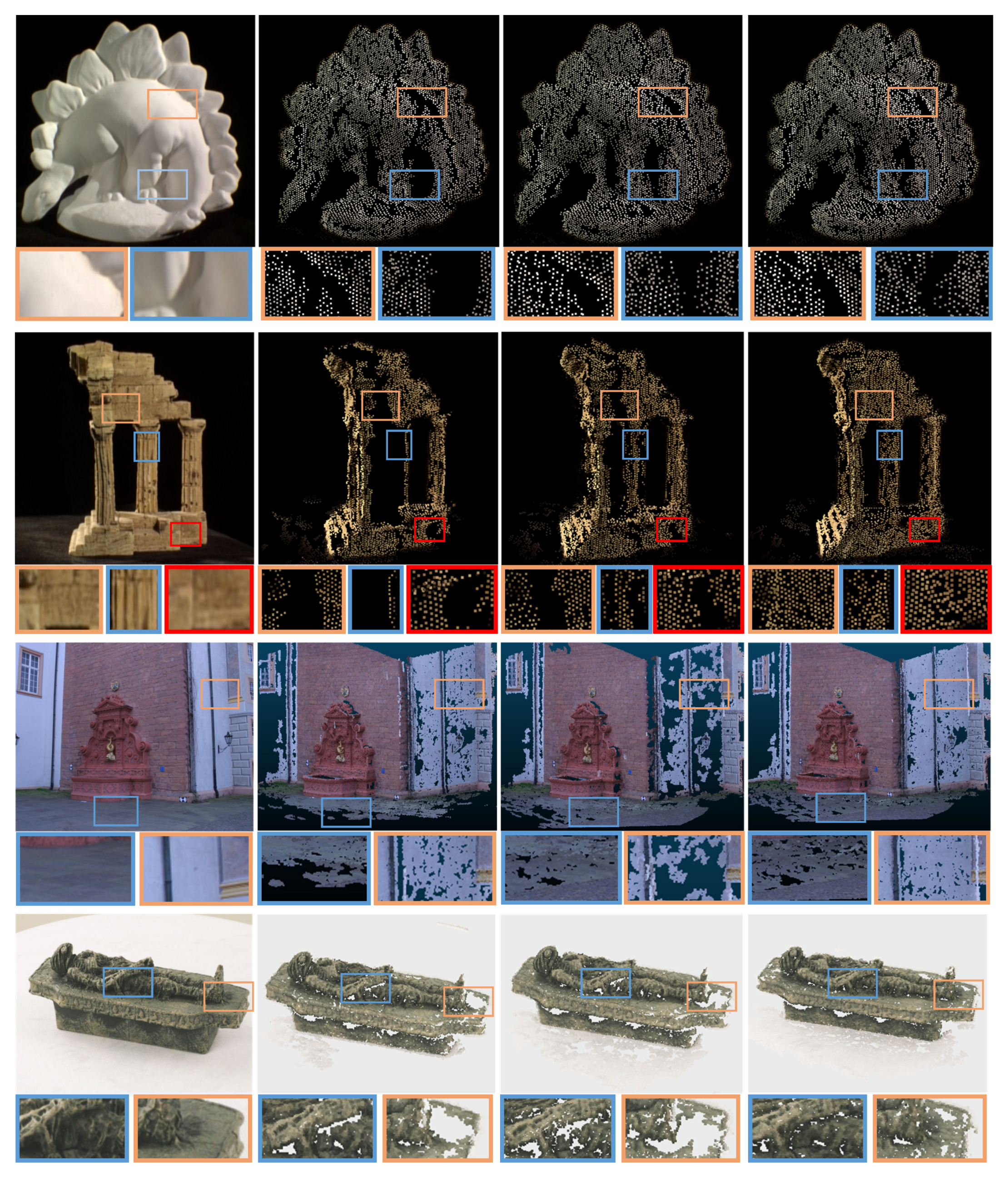
7.2. Evaluation of the Proposed Metric

The proposed similarity metric weakens the influences of textureless scenario and illumination difference in images, which can enhance the robustness to target properties and shooting conditions. To achieve fair evaluation, we compared the proposed algorithm with two other seed-and-expand schemes, PMVS [7] and VisualSfM [8]. PMVS initializes patches from retrieved sparse model points, and then propagates each seed patch to its neighborhoods by the mean photo-consistency of all visible pairs to recover a dense point cloud model. VisualSfM incorporates SfM and CMVS to implement optimized 3D reconstruction.

7.2.1. Textureless Scenarios

The comparisons are conducted on all ten datasets, and the samples of reconstructed results are demonstrated with local details magnified into view. Column 2/3/4 in Figure 6 respectively depict the reconstruction results from PMVS, VisualSfM, and ours. For model “Dino16”, “Temple16”, and “Mummy24”, the point clouds retrieved by the proposed method are more evenly distributed than that by PMVS or VisualSfM, such as the leg part of “Dino16”, the pillar of “Temple16”, and the feet area of “Mummy24”, outperforming the comparing algorithms in completeness and details. Despite VisualSfM’s results being partially better in a few small regions, such as the stairs of “Temple16” and head part of “Mummy24”, ours still gain more reliable reconstruction results than comparing methods. For textureless scenarios, such as the smooth back area of “Dino16”, the textureless wall area of “Fountain25”, and the white platform of “Mummy24”, the proposed method generates reasonable dense points in these areas, while PMVS and VisualSfM cause obvious local holes or incomplete surface, which shows the advantage of the proposed metric in dealing with textureless cases. These observations are also proved by the figures in

Table 2. Comparison of retrieved points and running time of three methods.

Image Sequences			Retrieved Points			Time (s)
Name	No.	Resolution	PMVS	VisualSfM	Ours	PMVS	VisualSfM	Ours
Dino16	16	640 × 480	8138	9036	8834	6	5	6
Dino48	48	640 × 480	9484	9528	9694	8	9	11
Dino363	363	640 × 480	32,030	34,462	33,869	51	63	60
Temple16	16	480 × 640	6997	7868	8458	5	7	6
Temple47	26	480 × 640	17,735	17,773	20,720	19	20	23
Mummy24	24	1600 × 1100	40,348	45,548	48,272	26	36	31
Fountain25	25	3072 × 2048	447,552	455,511	463,935	323	418	310
Stone39	39	3024 × 4032	618,829	562,521	624,971	756	890	786
Sculpture58	58	2592 × 1728	1,018,650	924,024	997,770	780	912	810
Statue70	70	1920 × 1080	61,311	67,825	75,688	87	101	97

, revealing that the proposed approach produces, on average, 10.0% more 3D points than PMVS and 6.0% than VisualSfM. In addition, our method outperforms VisualSfM in efficiency for larger datasets with more images and higher resolutions.

7.2.2. Differences in Illumination

To verify the robustness of proposed metric to shooting conditions, we simulated the illumination difference in images by varying the illumination of each input image via a random ratio in [$-\tau$, $\tau$]. The range factor $\tau$ is increased from 10% to 60% to present different degrees of illumination variation. Figure 7 depicts the results of the proposed method under different degree of illumination variations. For four testing datasets, our method achieves good reconstruction performance. The retrieved point cloud models under different illumination variations show the similar density. Compared with PMVS and VisualSfM, ours exhibits better robustness.

Figure 8 gives the curves of retrieved points to illumination variation by three methods. It is shown that PMVS and VisualSfM can not guarantee dense points in illumination varying scenarios, especially when the variation is severe. While the proposed method reveals better reliability and outperforms the comparing methods in such cases. On average, the proposed method recovers 12.7% more points than PMVS and 10.3% than VisualSfM on four testing models. To give intuitive comparison, the results of three methods under $\tau$ = 50% are illustrated. Figure 9a depicts the input images with illumination randomly altered, and Figure 9b–d demonstrate the corresponding reconstructed point cloud models by three methods. Ours obtains more complete (“Dino16” and “Foundation25”) or denser (“Mummy24” and “Temple47”) than other two methods under significant illumination variation.

7.3. Quantitative Evaluations

In this section, we present the quantitative evaluation of the proposed reconstruction method on “Qinghuamen” and “Shengkelou” datasets with ground-truth point clouds generated by the Robot Vision Group, National Laboratory of Pattern Recognition Institute of Automation, and Chinese Academy of Sciences [51].

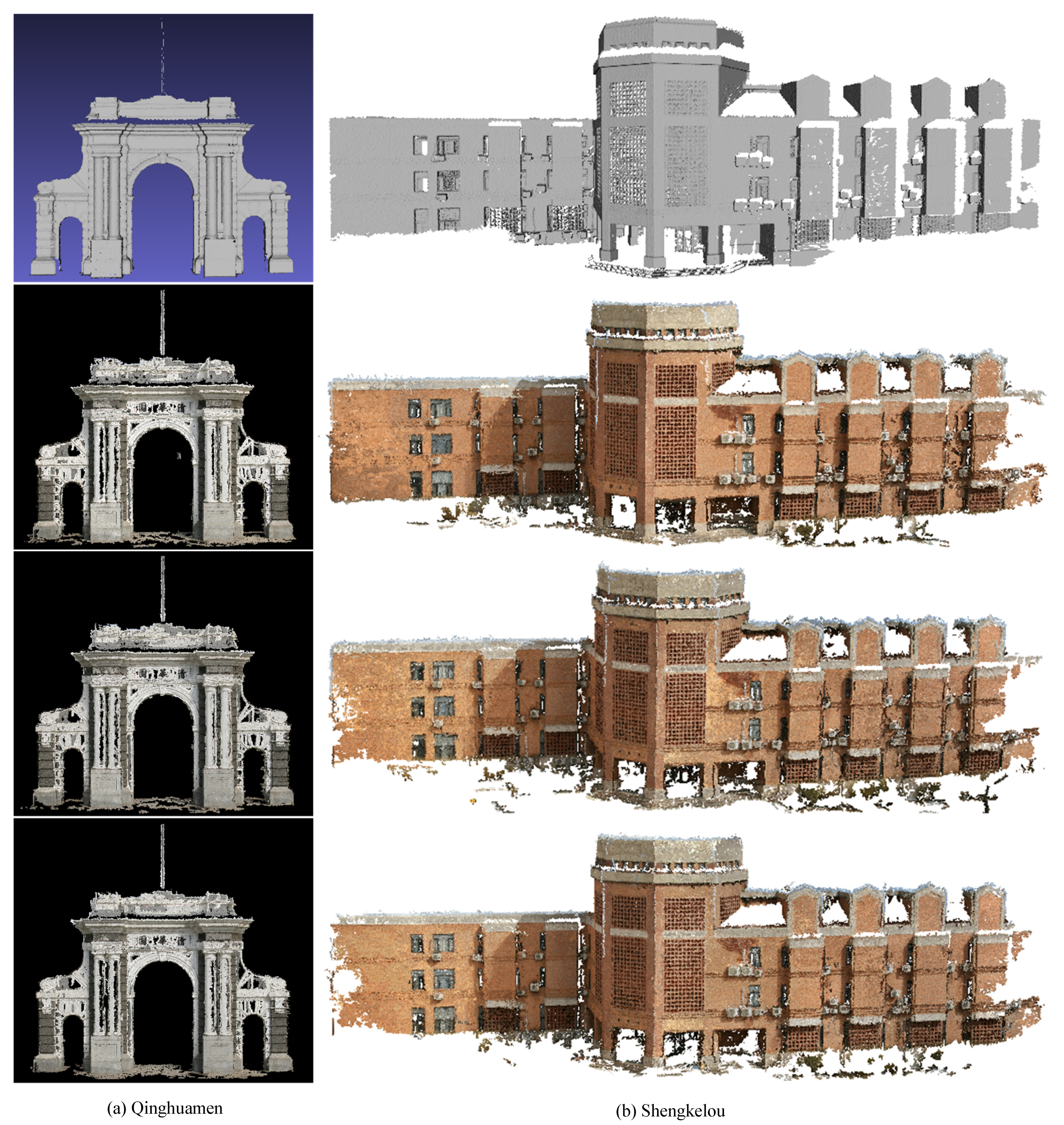
7.3.1. Completeness and Accuracy

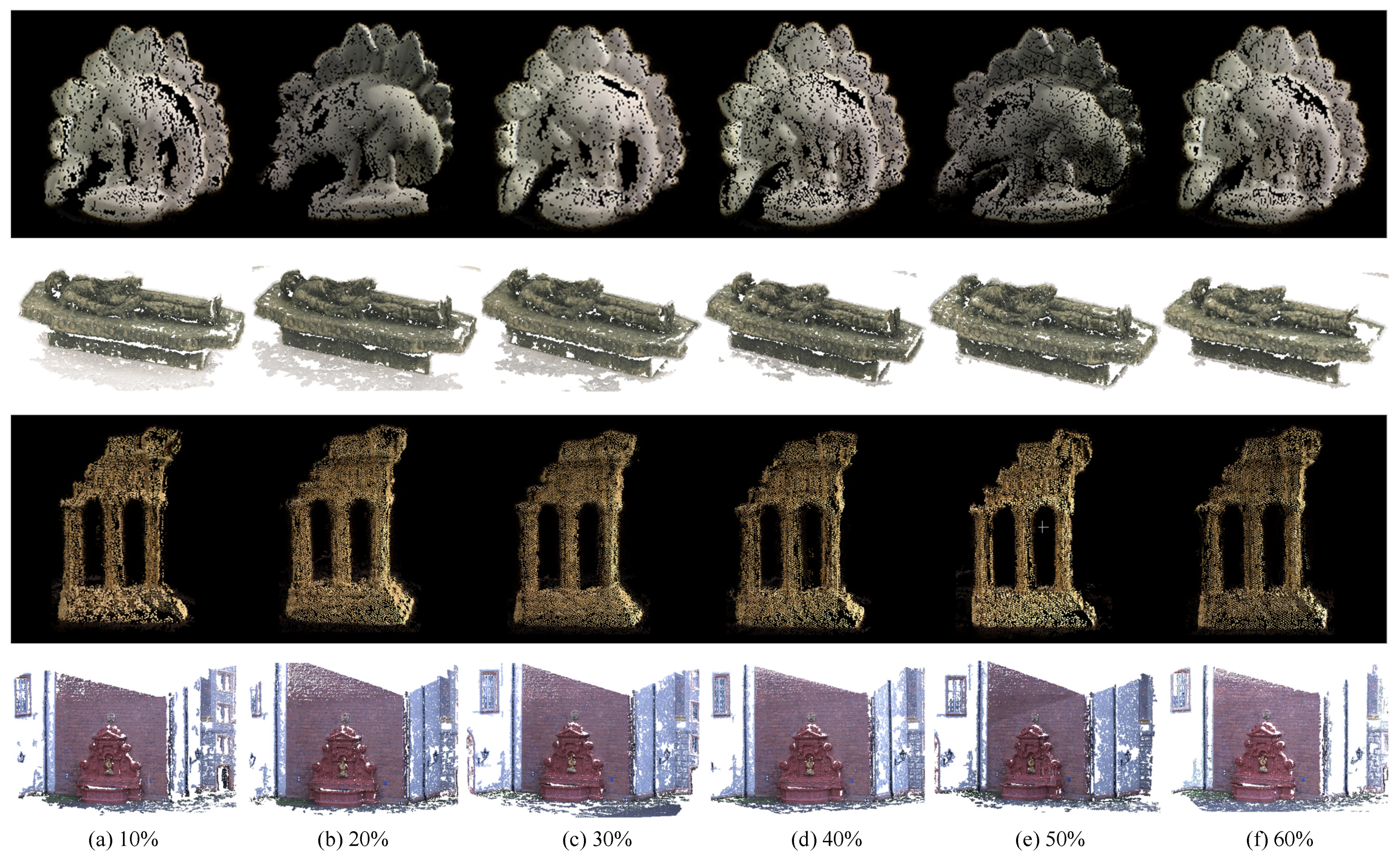
First, we fairly compare three methods in terms of completeness and accuracy, which are respectively defined as the percent of points that are within a threshold distance to the ground-truth and the average distance of reconstructed points to the ground-truth point cloud model [19].

Table 3. Quantitative results of the three algorithms on different datasets when $\tau$ = 50%. Bold number indicates the best result for each metric.

	Qinghuamen			Shengkelou			Shengkelou
	(68 Images, 4368 × 2912)			(102 Images, 4368 × 2912)			(51 Images, 4368 × 2912)
Method	Points	Comp.	Acc.	Points	Comp.	Acc.	Points	Comp.	Acc.
Ours	1,283,729	96.3%	0.001346	2,446,138	97.2%	0.004367	1,592,848	96.2%	0.004732
PMVS	1,270,131	96.1%	0.001379	2,382,383	97.0%	0.005221	1,592,127	95.6%	0.005696
VisualSfM	1,237,815	96.0%	0.001327	2,226,646	96.8%	0.004387	1,535,094	94.9%	0.004706

summarizes the results of completeness and accuracy metrics on the recovered point cloud models of three methods. For completeness, we use an inlier threshold of 0.05 m, i.e., a completeness of 95% means that 95% of the model is covered by the reconstructed points that are within 0.05 m to the ground-truth. Since we use average distance to the ground-truth as accuracy, a lower number implies higher accuracy. It is shown that the proposed method outperforms PMVS and VisualSfM in completeness under severe illumination variations ($\tau$ = 50%) while gaining similar accuracy to the other two methods, and completeness and accuracy decrease with fewer images on the “Shengkelou” dataset. The reconstructed models illustrated in Figure 10 match well to the numbers in Table 3. The proposed method achieves better completeness on both datasets, for instance, in the pillar area of “Qinghuamen” and the left part of the facade of “Shengkelou”, ours generates more points than PMVS and VisualSfM, leading to more complete models in illumination varying scenarios.

7.3.2. Parameters

In the last part of our experiments, we evaluate the impact of the parameters involved in the proposed metric on reconstructing completeness and accuracy. The evaluations are carried out on two datasets by arranging different settings of $\lambda$, ${\mu }_1$, ${\mu }_2$, ${\mu }_5$, $\epsilon$, and $\rho$.

Table 4. Evaluation results of the parameters involved in the proposed metric on different datasets when $\tau$ = 50%. Bold number indicates the best result for each metric.

Parameter Setting	Qinghuamen		Shengkelou		Shengkelou
	(68 Images)		(102 Images)		(51 Images)
$<\lambda ,{\mu }_1,{\mu }_2,{\mu }_5,\epsilon ,\rho >$	Comp.	Acc.	Comp.	Acc.	Comp.	Acc.
$\lambda$ = 0.3, ${\mu }_1$ = 0.8, ${\mu }_2$ = 0.6, ${\mu }_5$ = 0.7, $\epsilon$ = 1.0, $\rho$ = 2.25	96.0%	0.001419	97.1%	0.004916	96.1%	0.004759
$\lambda$ = 0.5, ${\mu }_1$ = 0.8, ${\mu }_2$ = 0.6, ${\mu }_5$ = 0.7, $\epsilon$ = 1.0, $\rho$ = 2.25	96.3%	0.001346	97.2%	0.004367	96.1%	0.004732
$\lambda$ = 0.5, ${\mu }_1$ = 0.7, ${\mu }_2$ = 0.5, ${\mu }_5$ = 0.6, $\epsilon$ = 1.0, $\rho$ = 2.25	96.4%	0.001442	96.9%	0.005034	96.2%	0.004914
$\lambda$ = 0.5, ${\mu }_1$ = 0.9, ${\mu }_2$ = 0.7, ${\mu }_5$ = 0.8, $\epsilon$ = 1.0, $\rho$ = 2.25	95.4%	0.001389	96.4%	0.004947	95.3%	0.004753
$\lambda$ = 0.5, ${\mu }_1$ = 0.8, ${\mu }_2$ = 0.6, ${\mu }_5$ = 0.7, $\epsilon$ = 0.5, $\rho$ = 2.25	96.1%	0.001394	96.9%	0.004257	95.9%	0.004907
$\lambda$ = 0.5, ${\mu }_1$ = 0.8, ${\mu }_2$ = 0.6, ${\mu }_5$ = 0.7, $\epsilon$ = 1.0, $\rho$ = 1.5	96.1%	0.001380	96.2%	0.003959	95.6%	0.004824

gives the quantitative results of different parameter settings. $\lambda$ controls the weight of illumination term in the proposed metric, and the numbers show that larger setting contributes to better completeness in illumination varying scenario, which is in line with its definition. Thresholds for correspondence diffusing, ${\mu }_1$, ${\mu }_2$, and ${\mu }_5$ weigh the qualification of feature matches for diffusion. The results reveal that a larger setting promotes the reconstruction accuracy at a the cost of a bit of completeness, and vice versa. $\epsilon$ and $\rho$ play similar roles in completeness and accuracy, only in an opposite direction.

It is observed that the numbers in Table 4 do not vary obviously as anticipated; this is because the high-resolution images counteract the influences of parameter variations, but the trend can be noticed. Overall, strict thresholds correspond to high accuracy but low completeness.

7.4. Discussion

Although our method achieves better model completeness and details in most cases, there are few occasions in which VisualSfM shows partially better results, such as the head part of “Mummy24” (Figure 6). This is because a different similarity metric is proposed in our work, which selects different seeds and diffuses under a new criterion, hence retrieving different 3D points. To observe the whole models, ours achieves superior completeness and point distribution, in both regular cases and illumination varying scenarios. We tested the robustness under several illumination variations, more points could be recovered, and the demonstrated point cloud models verifies the quantitative figures. For the reconstruction accuracy on three datasets (Table 3), ours shows comparative results with VisualSfM, and is a little behind on “Qinghuamen” and “Shengkelou (51 images)” but the difference is slight. However, the leading in model completeness for all three datasets is noteworthy. With more points being recovered in the models, the accuracy is impacted accordingly, which is a trade-off between completeness and accuracy. Comparing the corresponding point cloud models in Figure 10b, this cost in accuracy is worth it and acceptable.

8. Conclusions

Retrieving 3D information from images is a challenging topic in the computer vision community, which still suffers from the shortcomings in practical applications. This work presents an enhanced similarity metric for filtering feature matches or 3D patches in two-phase diffusions of seed-and-expand dense reconstruction. This metric combines the zero-mean normalized cross-correlation coefficients of illumination and texture to deal with illumination changes and textureless cases. Incorporated with other visual constraints and geometry consistency, the proposed method recovers reasonable dense 3D point cloud models in both structure complex and textureless regions for different image sequences. The method is robust to illumination varying scenarios and achieves better completeness with comparative reconstructing accuracy.

Available image-based dense reconstruction methods are capable of retrieving dense 3D surface points of a scene or an object with rich details. However, the recovered point cloud models by these methods inevitably contain scattered background information that are unnecessary to many applications. Manually deleting those redundant points is tedious work which requires great patience and care. A potential way is to enforce extra restriction on the interesting regions of images when extracting and expanding 3D information from them. This could be realized via foreground/background segmentation or saliency detection of images. By determining the silhouette of the target object and utilizing it in a dense diffusion process, the insignificant background points can be avoided. This will be our future research focus.

References

1. Huang, F.; Yang, H.; Tan, X.; Peng, S.; Tao, J.; Peng, S. Fast Reconstruction of 3D Point Cloud Model Using Visual SLAM on Embedded UAV Development Platform. Remote Sens. 2020, 12, 3308. [Google Scholar] [CrossRef]
2. Hu, S.R.; Li, Z.Y.; Wang, S.H.; Ai, M.Y.; Hu, Q.W. A Texture Selection Approach for Cultural Artifact 3D Reconstruction Considering Both Geometry and Radiation Quality. Remote Sens. 2020, 12, 2521. [Google Scholar] [CrossRef]
3. McCulloch, J.; Green, R. Conductor Reconstruction for Dynamic Line Rating Using Vehicle-Mounted LiDAR. Remote Sens. 2020, 12, 3718. [Google Scholar] [CrossRef]
4. Snavely, N.; Seitz, S.M.; Szeliski, R. Modeling the World from Internet Photo Collections. Int. J. Comput. Vis. 2008, 80, 189–210. [Google Scholar] [CrossRef] [Green Version]
5. Furukawa, Y.; Curless, B.; Seitz, S.M.; Szeliski, R. Towards Internet-scale multi-view stereo. In Proceedings of the IEEE Conference on Computer Vision and Pattern Recognition, San Francisco, CA, USA, 13–18 June 2010; pp. 1434–1441. [Google Scholar]
6. Yang, Y.; Liang, Q.; Niu, L.; Zhang, Q. Belief propagation stereo matching algorithm using ground control points. In Proceedings of the SPIE—The International Society for Optical Engineering, San Diego, CA, USA, 17–21 August 2014; Volume 9069, pp. 90690W-1–90690W-7. [Google Scholar]
7. Furukawa, Y. Multi-View Stereo: A Tutorial. Found. Trends Comput. Graph. Vis. 2015, 9, 1–148. [Google Scholar] [CrossRef] [Green Version]
8. Wu, C. VisualSFM: A Visual Structure From Motion System 2012. [Online]. Available online: http://homes.cs.washington.edu/~ccwu/vsfm (accessed on 31 July 2019).
9. Wu, P.; Liu, Y.; Ye, M.; Li, J.; Du, S. Fast and Adaptive 3D Reconstruction With Extensively High Completeness. IEEE Trans. Multimed. 2017, 19, 266–278. [Google Scholar] [CrossRef]
10. Schonberger, J.L.; Radenovic, F.; Chum, O.; Frahm, J.M. From single image query to detailed 3D reconstruction. In Proceedings of the Computer Vision and Pattern Recognition, Boston, MA, USA, 7–12 June 2015; pp. 5126–5134. [Google Scholar]
11. Huang, Q.; Wang, H.; Koltun, V. Single-view reconstruction via joint analysis of image and shape collections. ACM Trans. Graph. 2015, 34, 87. [Google Scholar] [CrossRef] [Green Version]
12. Yan, F.; Gong, M.; Cohen-Or, D.; Deussen, O.; Chen, B. Flower reconstruction from a single photo. Comput. Graph. Forum 2014, 33, 439–447. [Google Scholar] [CrossRef] [Green Version]
13. Chai, M.L.; Luo, L.J.; Sunkavalli, K.; Carr, N.; Hadap, S.; Zhou, K. High-quality hair modeling from a single portrait photo. ACM Trans. Graph. 2015, 34, 204. [Google Scholar] [CrossRef]
14. Eigen, D.; Puhrsch, C.; Fergus, R. Depth map prediction from a single image using a multi-scale deep network. In Proceedings of the International Conference on Neural Information Processing Systems, Montreal, QC, Canada, 8–13 December 2014; pp. 2366–2374. [Google Scholar]
15. Li, F.; Sekkati, H.; Deglint, J.; Scharfenberger, C.; Lamm, M.; Clausi, D.; Zelek, J.; Wong, A. Simultaneous Projector-Camera Self-Calibration for Three-Dimensional Reconstruction and Projection Mapping. IEEE Trans. Comput. Imaging 2017, 3, 74–83. [Google Scholar] [CrossRef]
16. Fraser, C.S. Automatic Camera Calibration in Close Range Photogrammetry. Photogramm. Eng. Remote. Sens. 2013, 79, 381–388. [Google Scholar] [CrossRef] [Green Version]
17. Li, Y.; Wang, S.; Tian, Q.; Ding, X. A survey of recent advances in visual feature detection. Neurocomputing 2015, 149, 736–751. [Google Scholar] [CrossRef]
18. Dehais, J.; Anthimopoulos, M.; Shevchik, S.; Mougiakakou, S. Two-View 3D Reconstruction for Food Volume Estimation. IEEE Trans. Multimed. 2017, 19, 1090–1099. [Google Scholar] [CrossRef] [Green Version]
19. Seitz, S.M.; Curless, B.; Diebel, J.; Scharstein, D.; Szeliski, R. A Comparison and Evaluation of Multi-View Stereo Reconstruction Algorithms. In Proceedings of the IEEE Computer Society Conference on Computer Vision and Pattern Recognition, New York, NY, USA, 17–22 June 2006; pp. 519–528. [Google Scholar]
20. Alexiadis, D.S.; Zarpalas, D.; Daras, P. Real-Time, Full 3D Reconstruction of Moving Foreground Objects From Multiple Consumer Depth Cameras. IEEE Trans. Multimed. 2013, 15, 339–358. [Google Scholar] [CrossRef]
21. Bradley, D.; Boubekeur, T.; Heidrich, W. Accurate multi-view reconstruction using robust binocular stereo and surface meshing. In Proceedings of the IEEE Conference on Computer Vision and Pattern Recognition, Anchorage, AK, USA, 23–28 June 2008; pp. 1–8. [Google Scholar]
22. Liu, Y.; Cao, X.; Dai, Q.; Xu, W. Continuous depth estimation for multi-view stereo. In Proceedings of the IEEE Conference on Computer Vision and Pattern Recognition, Miami, FL, USA, 20–25 June 2009; pp. 2121–2128. [Google Scholar]
23. Li, Z.; Wang, K.; Meng, D.; Xu, C. Multi-view stereo via depth map fusion: A coordinate decent optimization method. Neurocomputing 2016, 178, 46–61. [Google Scholar] [CrossRef]
24. Gargallo, P.; Sturm, P. Bayesian 3D Modeling from Images Using Multiple Depth Maps. In Proceedings of the IEEE Computer Society Conference on Computer Vision and Pattern Recognition (CVPR 2005), San Diego, CA, USA, 20–25 June 2005; Volume 2, pp. 885–891. [Google Scholar]
25. Fan, H.; Kong, D.; Li, J. Reconstruction of high-resolution Depth Map using Sparse Linear Model. In Proceedings of the International Conference on Intelligent Systems Research and Mechatronics Engineering, Zhengzhou, China, 11–13 April 2015; pp. 283–292. [Google Scholar]
26. Lasang, P.; Shen, S.M.; Kumwilaisak, W. Combining high resolution color and depth images for dense 3D reconstruction. In Proceedings of the IEEE Fourth International Conference on Consumer Electronics—Berlin, Berlin, Germany, 7–10 September 2014; pp. 331–334. [Google Scholar]
27. Lhuillier, M.; Quan, L. Match propagation for image-based modeling and rendering. IEEE Trans. Pattern Anal. Mach. Intell. 2002, 24, 1140–1146. [Google Scholar] [CrossRef]
28. Habbecke, M.; Kobbelt, L. A Surface-Growing Approach to Multi-View Stereo Reconstruction. In Proceedings of the IEEE Conference on Computer Vision and Pattern Recognition, CVPR ’07, Minneapolis, MN, USA, 17–22 June 2007; pp. 1–8. [Google Scholar]
29. Zhang, Z.; Shan, Y. A Progressive Scheme for Stereo Matching. In Revised Papers from Second European Workshop on 3D Structure from Multiple Images of Large-Scale Environments; Springer: Berlin/Heidelberg, Germany, 2000; pp. 68–85. [Google Scholar]
30. Cech, J.; Sara, R. Efficient Sampling of Disparity Space for Fast In addition, Accurate Matching. In Proceedings of the IEEE Conference on Computer Vision and Pattern Recognition, CVPR ’07, Minneapolis, MN, USA, 17–22 June 2007; pp. 1–8. [Google Scholar]
31. Goesele, M.; Snavely, N.; Curless, B.; Hoppe, H.; Seitz, S.M. Multi-View Stereo for Community Photo Collections. In Proceedings of the IEEE International Conference on Computer Vision, Rio de Janeiro, Brazil, 14–21 October 2007; pp. 1–8. [Google Scholar]
32. Snavely, N.; Seitz, S.M.; Szeliski, R. Photo Tourism: Exploring Photo Collections in 3D. In ACM SIGGRAPH; ACM: New York, NY, USA, 2006; pp. 835–846. [Google Scholar]
33. Furukawa, Y.; Ponce, J. Accurate, Dense, and Robust Multi-View Stereopsis. IEEE Trans. Pattern Anal. Mach. Intell. 2010, 32, 1362–1376. [Google Scholar] [CrossRef] [PubMed]
34. Tanskanen, P.; Kolev, K.; Meier, L.; Camposeco, F.; Saurer, O.; Pollefeys, M. Live Metric 3D Reconstruction on Mobile Phones. In Proceedings of the IEEE International Conference on Computer Vision, Sydney, Australia, 1–8 December 2013; pp. 65–72. [Google Scholar]
35. Snavely, N. Bundler: Structure from Motion (SfM) for Unordered Image Collections. July 2010. [Online]. Available online: http://phototour.cs.washington.edu/bundler (accessed on 20 June 2019).
36. Han, X.; Laga, H.; Bennamoun, M. Image-based 3D Object Reconstruction: State-of-the-Art and Trends in the Deep Learning Era. IEEE Trans. Pattern Anal. Mach. Intell. (Early Access) 2019. [Google Scholar] [CrossRef] [PubMed] [Green Version]
37. Park, J.J.; Florence, P.; Straub, J.; Newcombe, R.; Lovegrove, S. DeepSDF: Learning Continuous Signed Distance Functions for Shape Representation. In Proceedings of the IEEE CVPR, Long Beach, CA, USA, 15–20 June 2019; pp. 165–174. [Google Scholar]
38. Riegler, G.; Ulusoy, A.O.; Geiger, A. OctNet: Learning deep 3D representations at high resolutions. In Proceedings of the IEEE CVPR, Honolulu, HI, USA, 21–26 July 2017; Volume 3. [Google Scholar]
39. Nie, Y.Y.; Han, X.G.; Guo, S.H.; Zheng, Y.; Chang, J.; Zhang, J.J. Total3DUnderstanding: Joint Layout, Object Pose and Mesh Reconstruction for Indoor Scenes from a Single Image. In Proceedings of the CVPR, Seattle, WA, USA, 14–19 June 2020. [Google Scholar]
40. Pontes, J.K.; Kong, C.; Sridharan, S.; Lucey, S.; Eriksson, A.; Fookes, C. Image2Mesh: A Learning Framework for Single Image 3D Reconstruction. In Asian Conference on Computer Vision; Springer: Cham, Switzerland, 2018. [Google Scholar]
41. Li, K.; Pham, T.; Zhan, H.; Reid, I. Efficient dense point cloud object reconstruction using deformation vector fields. In Proceedings of the ECCV, Munich, Germany, 8–14 September 2018; pp. 497–513. [Google Scholar]
42. Wang, J.; Sun, B.; Lu, Y. MVPNet: Multi-View Point Re-gression Networks for 3D Object Reconstruction from A Single Image. Proc. AAAI Conf. Artif. Intell. 2018, 33, 8949–8956. [Google Scholar] [CrossRef]
43. Mandikal, P.; Murthy, N.; Agarwal, M.; Babu, R.V. 3D-LMNet: Latent Embedding Matching for Accurate and Diverse 3D Point Cloud Reconstruction from a Single Image. In Proceedings of the BMVC, Newcastle, UK, 3–6 September 2018; pp. 662–674. [Google Scholar]
44. Jiang, L.; Shi, S.; Qi, X.; Jia, J. GAL: Geometric Adversarial Loss for Single-View 3D-Object Reconstruction. In Proceedings of the ECCV, Munich, Germany, 8–14 September 2018. [Google Scholar]
45. Insafutdinov, E.; Dosovitskiy, A. Unsupervised learning of shape and pose with differentiable point clouds. In Proceedings of the NIPS, Montreal, QC, Canada, 3–8 December 2018; pp. 2802–2812. [Google Scholar]
46. Fan, H.; Su, H.; Guibas, L. A point set generation network for 3D object reconstruction from a single image. In Proceedings of the IEEE Conference on Computer Vision and Pattern Recognition, CVPR ’17, Honolulu, HI, USA, 21–26 July 2017; Volume 38. [Google Scholar]
47. Tatarchenko, M.; Dosovitskiy, A.; Brox, T. Multi-view 3D models from single images with a convolutional network. In Proceedings of the ECCV, Amsterdam, The Netherlands, 11–14 October 2016; pp. 322–337. [Google Scholar]
48. Lin, C.H.; Kong, C.; Lucey, S. Learning Efficient Point Cloud Generation for Dense 3D Object Reconstruction. In Proceedings of the AAAI, New Orleans, LA, USA, 2–7 February 2018. [Google Scholar]
49. Triggs, B.; Mclauchlan, P.F.; Hartley, R.I.; Fitzgibbon, A.W. Bundle Adjustment—A Modern Synthesis. In Proceedings of the ICCV ’99 Proceedings of the International Workshop on Vision Algorithms: Theory and Practice, Corfu, Greece, 21–22 September 1999; pp. 298–372.
50. Lowe, D.G. Distinctive Image Features from Scale-Invariant Keypoints. Int. J. Comput. Vis. 2004, 60, 91–110. [Google Scholar] [CrossRef]
51. Robot Vision Group, National Laboratory of Pattern Recognition Institute of Automation, Chinese Academy of Sciences. [Online]. Available online: http://vision.ia.ac.cn/data/ (accessed on 15 December 2020).
Figure 1. Flow chart of proposed dense reconstruction scheme for image sequence. It takes sequenced images as input and output 3D points via three stages: preprocessing, feature diffusion, and patch diffusion. The dashed boxes unfold the main steps of each stage. Refer to Section 3 for a detailed description.
Remotesensing 13 00567 g001
Figure 2. Feature match is diffused to its neighborhood pixels. For feature correspondence ( p 11 , q 22 ), build multi-to-multi matchings within the local windows W l and W r in its host images, then employ disparity gradient constraint and confidence measure to prune false matchings.
Remotesensing 13 00567 g002
Figure 3. Illustration of patch expansion. Case (b) depicts that the seed patch is propagated to its neighboring cell since no similar patch occupies it. Case (a) and (c) are the non-propagation scenarios where the patch in the neighboring cell is close to or shares a high similarity value with the seed patch.
Remotesensing 13 00567 g003
Figure 4. Illustration of the reconstruction result of proposed dense diffusion algorithm on three datasets, “Dino16”, “Temple16” and “Fountain25”. From left to right: sample of image sequence, feature diffusion results, patch diffusion results.
Remotesensing 13 00567 g004
Figure 5. Results of proposed algorithm on other four datasets. Top: “Mummy24” and “Sclupture58”. Bottom: “Statue70” and “Stone39”. Left: sample of image sequence. Right: retrieved point cloud.
Remotesensing 13 00567 g005
Figure 6. Comparison of three reconstruction methods on four testing datasets. From top to bottom: “Dino16”, “Temple16”, “Fountain25”, and “Mummy24”. From left to right: sample of image sequence, the results by PMVS, VisualSfM, and ours. The local details are highlighted and magnified into view. Ours generates reasonable dense points in textureless areas, e.g., the smooth back area of “Dino16”, the wall area of “Fountain25”, and the white platform of “Mummy24”.
Remotesensing 13 00567 g006
Figure 7. The reconstructing models of proposed method under different illumination variations of input images. The controlling factor τ varies from 10% to 60% (from left to right) and the reconstructed point cloud models are illustrated. Top to bottom: “Dino16”, “Mummy24”, “Temple47”, “Foundation25”.
Remotesensing 13 00567 g007
Figure 8. Comparison of the recovered points by three reconstruction methods under different illumination variations (10% to 60%). Four datasets are tested and they are (ad): “Dino16”, “Mummy24”, “Temple47”, and “Foundation25”.
Remotesensing 13 00567 g008
Figure 9. Comparison of recovered point cloud models by three reconstruction methods when the controlling factor τ of illumination change is 50%. (a) input images with illumination randomly altered; (bd) the results from PMVS, VisualSfM, and ours. Top to bottom: “Dino16”, “Mummy24”, “Temple47”, “Foundation25”.
Remotesensing 13 00567 g009
Figure 10. Comparison of recovered point cloud models by the three reconstruction methods when τ = 50%. (a) “Qinghuamen”(68 images, 4368 × 2912), (b) “Shengkelou”(102 images, 4368 × 2912). Top to bottom: ground-truth, ours, PMVS, VisualSfM. In the pillar area of “Qinghuamen” and the left part of the facade of “Shengkelou”, ours generates more points than PMVS and VisualSfM.
Remotesensing 13 00567 g010