Time-Frequency Reversion-Based Spectrum Analysis Method and Its Applications in Radar Imaging

Abstract

Spectrum analysis (SA) plays an important role in radar signal processing, especially in radar imaging algorithm design. Because it is usually hard to obtain the analytical expression of spectrum by the Fourier integral directly, principle of stationary phase (POSP)-based SA is applied to approximate this integral. However, POSP requires the phase of the signal to vary rapidly, which is not the case in circular synthetic aperture radar (SAR) and turntable inverse SAR (ISAR). To solve this problem, a new SA method based on time-frequency reversion (TFRSA) is proposed, which utilizes the relationship of the Fourier transform pairs and their corresponding signal phases. In addition, the connection between the imaging geometry and time-frequency relationship is also analyzed and utilized to help solve the time-frequency reversion. When the TFRSA is applied to the linear trajectory SAR, the obtained spectrum expression is the same as the result of POSP. When it is applied to ISAR, the spectrum expressions of near-field and far-field are derived and their difference is found to be position-independent. Based on this finding, an extended polar format algorithm (EPFA) for near-field ISAR imaging is proposed, which can solve the distortion and defocusing problems caused by traditional ISAR imaging algorithms. When it is applied to the circular SAR (CSAR), a new and efficient imaging method based on EPFA is proposed, which can solve the low efficiency problem of conventional BP-based CSAR imaging algorithms. The simulations and real data processing results are provided to validate the effectiveness of proposed method.

1. Introduction

Radar can realize long distance target detection, localization, imaging, classification and recognition in all-day and all-weather conditions, and has become a significant tool in many applications. Among these applications, Synthetic aperture radar (SAR) [1,2,3] and inverse SAR (ISAR) [4,5,6] imaging attracted much attention, because they can provide two-dimension high-resolution images, which contain many features, for example, the size and shape. Different from optical imaging, radar imaging produces images by complex computation. The resolution of radar image in the range dimension is accomplished by transforming the large signal bandwidth, whereas the fine resolution in azimuth stems from the difference in observation angles. With the development of advanced hardware, the available radar bandwidth is becoming larger, which in turn produces ultrahigh-resolution radar images. Recently, the microwave-photonic technique [7,8,9], which combines the advantages of electromagnetic wave and photonics techniques, is applied to the radar system to produce an ultra-large 10 GHz bandwidth radar signal. This microwave-photonic radar can generate radar images with 1.5 cm resolutions [10,11]. In addition to the large bandwidth, wide-angle radar imaging is also a worthwhile study direction, because it can not only produce ultrahigh azimuth resolution but also provide anisotropy characteristic, which is very useful for target classification and recognition.

The design of radar imaging algorithm is usually based on the spectrum of the radar received signal [3]. Different constructions of virtual synthetic apertures always lead to different imaging algorithms. Thus, the spectrum analysis (SA) is very important to radar imaging. The Fourier integral is a direct way to perform SA. However, the integral is usually difficult to evaluate, and approximation is often applied to obtain the Fourier integral. Principle of stationary phase (POSP) is one of the popular methods used for asymptotic analysis [12]. Because the phase of the radar signal changes rapidly, the cancellation of sinusoids would cause the integral to be zero except near the stationary point. Due to its simplicity, POSP is widely used in radar signal processing and imaging algorithm design [13,14,15], especially for the linear trajectory SAR (LTSAR). Because the phase is assumed to be changing rapidly, POSP is considered applicable when the signal’s time and bandwidth product (TBP) is larger than 100, which is satisfied in most of the LTSAR applications.

For curved trajectory SAR (CTSAR), like the circular SAR (CSAR), the TBP condition cannot be satisfied for returns of scatterers near the scene center, and thus POSP cannot be applied to CSAR. This leads to the difficulty of obtaining the spectrum expression and designing efficient Doppler domain imaging algorithm for CSAR. Back-projection algorithm (BPA) is a well-known and accurate time-domain imaging algorithm, which is applicable to any trajectories of SAR. However in BPA, the value of every image pixel is calculated by integrating using the accurate slant range, this incurs huge computational costs. In order to improve the efficiency of imaging, many accelerated BPAs are proposed [16,17]. However, their efficiencies are still not comparable to that of frequency-domain algorithms, for example, chirp scaling algorithm (CSA), frequency scaling algorithm (FSA), and range migration algorithm (RMA) [3].

Different from SAR, which usually observes the stationary scene by moving the radar along the predesigned trajectory, ISAR usually observes non-cooperative moving targets in the static platform, which means its corresponding virtual synthetic aperture is more complex and this leads to complicated Doppler spectrum. In traditional ISAR imaging, the distance between the radar and target is usually considered much larger than the size of the target. Thus, the plane wave assumption is applied to decompose the slant range into the two uncoupled parts: translational motion (TM) and rotational motion (RM). TM is the same for all scatterers of the target and has no contribution to ISAR imaging. There are many methods proposed to compensate the TM to produce an equivalent turntable model for ISAR imaging [18,19,20]. Moreover, many imaging algorithms were proposed for the turntable ISAR imaging under the plane wave assumption, for example, the range-Doppler algorithm (RDA), keystone transform (KT)-based imaging algorithm, and polar format algorithm (PFA) [5].

However, with the increasing demand for finer image resolution, the accuracy requirement of error compensation for radar imaging has also increased. Besides, the distance between radar and target for some applications are becoming smaller, for example, target detection and ranging for autonomous vehicles, harbor surveillances, and airport security checks [21,22,23]. In these situations, termed near-field ISAR imaging, the plane wave assumption may not be accurate enough for high-resolution ISAR imaging and the corresponding image quality would be degraded. In the near-filed situations, traditional ISAR imaging algorithms, like KT-based method and PFA, would produce images with geometric distortion and defocusing problems. Besides, for the near-field turntable ISAR, where a target is placed on a turntable with only rotational motion, the POSP is also inapplicable because the returns of the scatterers near the turntable center are narrow-band signals.

In order to overcome the limitations of POSP, a new SA method based on time-frequency reversion (TFR) is proposed in this paper. By utilizing the relationship between the Fourier transform (FT) pairs and their corresponding signal phases, the frequency-time distributed lines (FTDL) [24,25] can be obtained and the spectrum can be evaluated by integrating the FTDL. Besides, the connection between the time-frequency relationship and the imaging geometry is also analyzed, leading to a simplification of the time-frequency reversion process, and at the same time, providing a physical insight of the problem. When the proposed TFR-based spectrum analysis (TFRSA) method is applied to LTSAR, the derived spectrum expression is the same as the result of POSP, which validates the accuracy of TFRSA. When TFRSA is applied to the near-field ISAR, its spectrum expression is also derived. It is worth noting that the derived difference between near-field and far-field spectrums is a position-independent expression. With this finding, an extended polar format algorithm (EPFA) is proposed for the near-field ISAR imaging. When the TFRSA is applied to the CSAR, its spectrum is approximated to a near-field ISAR spectrum with position-dependent constant error, and an efficient CSAR imaging algorithm is proposed based on the EPFA.

The remainder of the paper is organized as follows. In Section 2.1, the signal model and adopted imaging geometry are given. In Section 2.2, the proposed TFRSA method is introduced. In Section 2.3, the TFRSA is applied to the LTSAR to derive its spectrum expression and this expression is compared with the result of POSP. In Section 2.4, the TFRSA is applied to the near-field ISAR to derive its spectrum expression and an EPFA is also proposed for near-field ISAR imaging. In Section 2.5, the TFRSA is applied to the CSAR, an efficient imaging method based on EPFA is proposed for CSAR. In Section 3, simulations and real data processing results are provided to validate the effectiveness of the proposed TFRSA and EPFA imaging methods. In Section 4, an explanation on the performances of different algorithms is given and the future research directions are also discussed. Finally, a conclusion is given in Section 5.

2. Materials and Methods

2.1. Radar Imaging Geometry and Signal Model

Different from optical imaging, which is based on the accumulation of photons, radar imaging produces images by complex computation. Radar transmits electromagnetic wave and receives the returns and samples them into digital data. Then, imaging processing is applied to the digital data to generate a radar image.

For SAR, its imaging geometry is illustrated in Figure 1a, in which radar is observing the static scene and moving along a predesigned trajectory. A Cartesian coordinate system $XOY$ is built on the imaging plane, which is defined by the radar velocity vector and the line of sight (LOS) vector. The origin is set at the center of the scene. The observation angle $\theta$ of radar is defined by the angle between the radar position vector and the Y-axis, which is demonstrated in Figure 1a. The i-th scatterer on the ground, whose coordinates are $\left(x_i^g,y_i^g\right)$ on the ground coordinate system $X_{g}O{Y}_g$, is projected onto the imaging plane with the coordinates $\left(x_i,y_i\right)$. Thus, the slant range between radar and i-th scatterer in the scene can be expressed as

$$\begin{array}{cc}\hfill R_i^{SAR}\left(\theta \right)& =\sqrt{{\left(r\left(\theta \right)cos\theta -y_i\right)}^2+{\left(r\left(\theta \right)sin\theta -x_i\right)}^2}\hfill \\ & =\sqrt{r^2\left(\theta \right)-2r\left(\theta \right)\left(x_{i}sin\theta +y_{i}cos\theta \right)+x_i^2+y_i^2},\hfill \end{array}$$

(1)

where $r\left(\theta \right)$ denotes the distance between the radar and the origin.

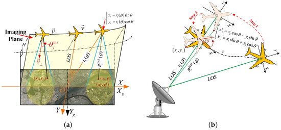
Figure 1. Radar imaging geometry. (a) Synthetic aperture radar (SAR) imaging geometry. (b) Inverse synthetic aperture radar (ISAR) imaging geometry.

For ISAR, its imaging geometry is illustrated in Figure 1b, in which the target is moving along arbitrary trajectory whereas the radar is static. In this case, the origin of the Cartesian coordinate system is set at the target center and the Y-axis is set parallel to the LOS. The motion of the target can be decomposed into two parts of rotation motion and radial translation, which corresponding to RM and TM, respectively. In order to express the rotational angle between two different positions of the target, the coordinate system $X_{1}O{Y}_1$ is first rotated to be parallel with $XOY$, which is demonstrated by step 1 in Figure 1b. Then, $X_{1}O{Y}_1$ is moved along the LOS to overlap with $XOY$, which is demonstrated by step 2. The rotational angle is defined by the $\vartheta$ demonstrated in Figure 1b. For the i-th scatterer in the target, its slant range can be expressed by

$$\begin{array}{cc}\hfill R_i^{ISAR}\left(\vartheta \right)& =\sqrt{{\left(r\left(\vartheta \right)-x_{i}sin\vartheta -y_{i}cos\vartheta \right)}^2+{\left(x_{i}cos\vartheta -y_{i}sin\vartheta \right)}^2}\hfill \\ & =\sqrt{r^2\left(\vartheta \right)-2r\left(\vartheta \right)\left(x_{i}sin\vartheta +y_{i}cos\vartheta \right)+x_i^2+y_i^2}\hfill \end{array},$$

(2)

where $r\left(\vartheta \right)$ denotes the distance between radar and the target center and $\left(x_i,y_i\right)$ depicts the coordinates of the i-th scatterer on the target when the rotational angle is 0. Comparing Equation (1) with Equation (2), we see that they have the same form, which means they are equivalent and they can be transformed into each other. Thus, for convenience, in the followings, we only take SAR for an example to introduce the signal model.

Assuming that radar transmits linear frequency modulation (LFM) signal and there are K scatterers, after down conversion and range compression, the received signal in range wavenumber and azimuth angle domain can be expressed as [26]

$$\begin{array}{cc}\hfill s\left(k_r,\theta \right)& =\sum _{i=1}^K{A}_{i}rect\left[\frac{k_r}{\mathsf{\Delta }{k}_r}\right]exp\left(-j{k}_r{R}_i\left(\theta \right)\right)\hfill \\ & =\sum _{i=1}^K{A}_{i}rect\left[\frac{k_r}{\mathsf{\Delta }{k}_r}\right]exp\left(-j{k}_r\sqrt{r^2\left(\theta \right)-2r\left(\theta \right)\left(x_{i}sin\theta +y_{i}cos\theta \right)+x_i^2+y_i^2}\right),\hfill \end{array}$$

(3)

where $A_i$ signifies the back scatter coefficient of the i-th scatterer, $rect\left[ \right]$ represents the rectangular window, and $k_r$ and $\mathsf{\Delta }{k}_r$ denote the range wavenumber and range wavenumber bandwidth, respectively. The angle $\theta$ is an azimuth variable and it can also be replaced by other azimuth variables like azimuth time t or azimuth radar position $X_r$ in the specific situations. The signal spectrum of the radar returns in this paper refers to applying azimuth FT along the azimuth variable of the signal in Equation (3).

2.2. Time-Frequency Reversion-Based Spectrum Analysis Method

Assuming $\theta$ is a function of azimuth time t and it is expressed as $\theta \left(t\right)$, we can rewrite Equation (3) using the azimuth variable t as

$$s\left(k_r,t\right)=\sum _{i=1}^K{A}_{i}rect\left[\frac{k_r}{\mathsf{\Delta }{k}_r}\right]exp\left(-j{k}_r\sqrt{r^2\left(t\right)-2r\left(t\right)\left(x_{i}sin\theta \left(t\right)+y_{i}cos\theta \left(t\right)\right)+x_i^2+y_i^2}\right),$$

(4)

By performing azimuth FT for the variable t, the Doppler spectrum of Equation (4) can be obtained by

$$S\left(k_r,f_D\right)=\int s\left(k_r,t\right)exp\left(-j2\pi f_{D}t\right)dt,$$

(5)

where $f_D$ signifies the Doppler frequency. Because the Fourier integral in Equation (5) is usually difficult to evaluate, an approximation is often applied to Equation (5) to obtain a simple result.

POSP is one of the common techniques to make this approximation. The main idea of POSP relies on the cancellation of sinusoids with rapidly varying phases. The phase of the radar signal usually changes rapidly due to the high carrier frequency, so the POSP is suitable for radar signal processing and it is widely used in SAR imaging applications, for instance, the FT of the LFM signal and LTSAR Doppler spectrum analysis.

Taking the FT for an example, assuming the analyzed signal is expressed as

$$g\left(t\right)=A\left(t\right)exp\left[j\phi \left(t\right)\right],$$

(6)

where $A\left(t\right)$ and $\phi \left(t\right)$ stand for the amplitude and phase of the signal $g\left(t\right)$, respectively, and the FT of $g\left(t\right)$ in Equation (6) can be evaluated by

$$\begin{array}{cc}\hfill S\left(\omega \right)& =\int A\left(t\right)exp\left[j\phi \left(t\right)\right]exp\left(-j\omega t\right)dt\hfill \\ & =\int A\left(t\right)exp\left[j\left(\phi \left(t\right)-\omega t\right)\right]dt\hfill \\ & =\int A\left(t\right)exp\left[j\varphi \left(t\right)\right]dt,\hfill \end{array}$$

(7)

where $\omega$ signifies the frequency variable. Assuming the stationary phase point of Equation (7) is $t=t^{*}$ and approximating the phase term $\varphi \left(t\right)$ by its second-order Taylor series, which yields

$$\varphi \left(t\right)\approx \left[\phi \left(t^{*}\right)-\omega t^{*}\right]+\frac{1}{2}{\phi }^{″}\left(t^{*}\right){\left(t-t^{*}\right)}^2,$$

(8)

where $\varphi$ denotes the second derivative of $\varphi \left(t\right)$ about t. By applying the POSP to the integral of Equation (7), the result can be expressed by

$$\begin{array}{cc}\hfill S\left(\omega \right)& \approx \int A\left(t^{*}\right)exp\left[j\left(\phi \left(t^{*}\right)-\omega t^{*}\right)+j\frac{1}{2}{\phi }^{″}\left(t^{*}\right){\left(t-t^{*}\right)}^2\right]dt\hfill \\ & =\sqrt{\frac{2\pi }{\left|{\varphi }^{″}\left(t^{*}\right)\right|}}A\left(t^{*}\right)exp\left[j\left(\phi \left(t^{*}\right)-\omega t^{*}\pm \frac{\pi }{4}\right)\right],\hfill \end{array}$$

(9)

where $\sqrt{\frac{2\pi }{\left|{\varphi }^{″}\left(t^{*}\right)\right|}}$ is a constant number and it is often ignored. From Equation (9) we find that POSP can simplify the FT integral and produce good approximated result, so it is widely used in radar signal processing.

However, the phase of the radar signal does not always change rapidly, for example, the returns of the CSAR and turntable ISAR. In these cases, the POSP would cause large error and the analyzed results are unusable. In order to solve this problem, we propose a new TFRSA method, which utilizes the relationship of the Fourier pairs and their corresponding signal phase. Here, we take the Fourier pairs of time and frequency as an example. The frequency can be expressed as the derivative of the signal phase of Equation (6), which is given by

$$\omega =\frac{d\phi \left(t\right)}{dt}={\phi }^{\prime }\left(t\right),$$

(10)

where $\phi$ depicts the derivative of the signal phase. Equation (10) is also called the time-frequency distribution lines (TFDL) [24,25], which is used to describe the characteristic of the signal. Moreover, for the spectrum of Equation (7), the time can also be expressed by the negative derivative of its phase, which is given by

$$t\left(\omega \right)=-\frac{d{\phi }^S\left(\omega \right)}{d\omega },$$

(11)

where ${\phi }^S\left(\omega \right)$ stands for the phase of the signal spectrum. Equation (11) is also called the FTDL. TFDL can be regarded as a 90 degrees rotation of the FTDL [27,28], which means that we can obtain the FTDL from the TFDL. Then, the spectrum phase can be calculated by integrating the FTDL along the frequency variable $\omega$, which yields

$${\phi }^S\left(\omega \right)=\int -t\left(\omega \right)d\omega =\int {{\phi }^{\prime }}^{-1}\left(\omega \right)d\omega ,$$

(12)

where ${{\phi }^{\prime }}^{-1}\left(\omega \right)$ denotes the inverse function of ${\phi }^{\prime }\left(t\right)$. Because the amplitude $A\left(t\right)$ is a low-frequency narrow band signal, and its FT can be regarded as an impulse function near the zero frequency, its effect on the signal spectrum can be regarded as a constant number and it is often ignored. This spectrum analysis method is called TFRSA. Furthermore, the FTDL can also be obtained from the imaging geometry, which utilizes the relationship between the instantaneous squint angle (ISA) and the spectrum variable. The ISA of the i-th scatterer is defined as the angle between the normal vector ${\overrightarrow{v}}_{\perp }$ of radar velocity and the vector from radar pointing to the scatterer, which is illustrated in Figure 1a. The ISA can also be expressed by the spectrum variable as follows

$$f_D^i=-\frac{2v^{ins}}{\lambda }sin{\theta }_i^{ins}\hspace{1em}\Rightarrow \hspace{1em}sin{\theta }_i^{ins}=-\frac{\lambda f_D^i}{2v^{ins}},$$

(13)

where $f_D^i$ and ${\theta }_i^{ins}$ depict the Doppler frequency and the ISA of the i-th scatterer, respectively, $\lambda$ and $v^{ins}$ signify the wavelength of the transmitted signal and the instantaneous velocity of the radar, respectively. Equation (13) reveals that there is a one-to-one mapping relationship between frequency and ISA. Combing the geometry relationship and Equation (13) can help us simplify the spectrum derivation and have a better understanding of the TFRT. In the following, we will apply the TFRSA to three specific applications to validate its effectiveness.

2.3. Linear Trajectory SAR Spectrum Analysis Based on TFRSA

Linear trajectory sweep mode is one of the most common modes in the SAR, and its spectrum result has been well studied by the POSP and validated in many applications. In this subsection, we apply the TFRSA to the LTSAR and compare the derived spectrum with the result of POSP. The imaging geometry of the LTSAR is illustrated in Figure 2. Here, we use the radar azimuth position $X_r$ as the azimuth variable and the corresponding spectrum azimuth variable is the azimuth wavenumber $k_x$. From the geometry relationship in Figure 2, the ISA of the i-th scatterer can be expressed as

$$tan{\theta }_i^{ins}=\frac{X_r-x_i}{R_b-y_i},$$

(14)

where $R_b$ signifies the range between the scene center and the linear trajectory. Using the spectrum azimuth variable $k_x$ to express the ISA and it yields

$$tan{\theta }_i^{ins}=\frac{-k_x}{\sqrt{k_r^2-k_x^2}},$$

(15)

where the radial wavenumber vector is parallel to the line from the radar pointing to the scatterer and the azimuth wavenumber vector is parallel to the radar velocity. Combining Equations (14) and (15), we can obtain

$$X_r\left(k_x\right)=\left(R_b-y_i\right)\frac{-k_x}{\sqrt{k_r^2-k_x^2}}+x_i,$$

(16)

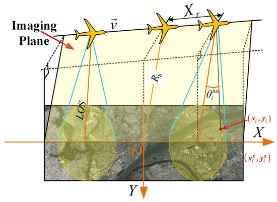
Figure 2. Imaging geometry of linear trajectory SAR.

The phase of the spectrum can be calculated by

$${\phi }^S\left(k_x\right)=\int -X_r\left(k_x\right)d{k}_x=\int \left(\left(R_b-y_i\right)\frac{k_x}{\sqrt{k_r^2-k_x^2}}-x_i\right)d{k}_x=-\sqrt{k_r^2-k_x^2}\left(R_b-y_i\right)-k_x{x}_i,$$

(17)

So, the spectrum derived by TFRSA is

$$S\left(k_r,k_x\right)=\sum _{i=1}^K{A}_{i}rect\left[\frac{k_r}{\mathsf{\Delta }{k}_r}\right]exp\left[-j\left(\sqrt{k_r^2-k_x^2}\left(R_b-y_i\right)+k_x{x}_i\right)\right],$$

(18)

Equation (18) is the same as the result derived by the POSP [3], which means the TFRSA has the same accuracy as POSP for LTSAR, but it is easier to understand physically. In the following, the TFRTAR is applied to the situations where POSP cannot be used, which are near-field ISAR and CSAR applications.

2.4. Near-Field ISAR Spectrum Analysis Based on TFRSA and EPFA for Near-Field ISAR Imaging

Because the plane wave assumption is not valid in the near-field ISAR, the traditional ISAR imaging algorithm would cause distortion and defocusing for near-field ISAR imaging. To solve these problems, a new imaging algorithm should be designed based on the spectrum of the near-field ISAR. For simplicity, here we take the turntable near-field ISAR as an example to analyze its spectrum. The geometry of the near-field ISAR is demonstrated in Figure 3 and the slant range of i-th scatterer in the target can be expressed by

$$R_i^{NF}\left(\vartheta \right)=\sqrt{{\left(R_0-x_{i}sin\vartheta -y_{i}cos\vartheta \right)}^2+{\left(x_{i}cos-y_{i}sin\vartheta \right)}^2},$$

(19)

where $R_0$ stands for the distance between the radar and the turntable center. From the geometry given in Figure 3, we can calculate the ISA of the i-th scatterer by

$$tan{\theta }_i^{ins}=\frac{-\left(x_{i}cos\vartheta -y_{i}sin\vartheta \right)}{R_0-x_{i}sin\vartheta -y_{i}cos\vartheta },$$

(20)

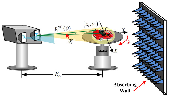
Figure 3. Imaging geometry of near-field ISAR.

Because the relationship of Equation (15) still holds here, by combining Equations (15) and (20), we can obtain

$$\frac{-\left(x_{i}cos\vartheta -y_{i}sin\vartheta \right)}{R_0-x_{i}sin\vartheta -y_{i}cos\vartheta }=\frac{-k_x}{\sqrt{k_r^2-k_x^2}},$$

(21)

Thus, the rotational angle $\vartheta$ can be expressed by the azimuth wavenumber $k_x$ as

$${\vartheta }^{NF}\left(k_x\right)=arccos\left(\frac{R_0{k}_x}{k_r\sqrt{x_i^2+y_i^2}}\right)+arctan\left(\frac{x_i{k}_x-y_i\sqrt{k_r^2-k_x^2}}{y_i{k}_x+x_i\sqrt{k_r^2-k_x^2}}\right),$$

(22)

where $arccos\left( \right)$ and $arctan\left( \right)$ signify the arccosine and arctangent functions.

We perform FT on the rotation angle $\vartheta$ with the angular wavenumber $\zeta$ as a variable. Transforming the imaging geometry of near-field ISAR into the CSAR imaging geometry means that the radar is moving along a circle centered at the turntable. Then, the relationship between radar aperture position $X_r$ and rotational angle $\vartheta$ is $X_r=R_0\vartheta$. According to the property of FT, the relationship between $\zeta$ and $k_x$ can be expressed by

$$k_x=\zeta /R_0 \Rightarrow \zeta =k_x{R}_0,$$

(23)

Substituting Equation (23) into Equation (22), the rotational angle can be rewritten as

$${\vartheta }^{NF}\left(\zeta \right)=arccos\left(\frac{\zeta }{k_r\sqrt{x_i^2+y_i^2}}\right)+arctan\left(\frac{x_i\zeta -y_i\sqrt{R_0^2{k}_r^2-{\zeta }^2}}{y_i\zeta +x_i\sqrt{R_0^2{k}_r^2+{\zeta }^2}}\right),$$

(24)

The spectrum phase of the near-field ISAR can be calculated by

$$\begin{array}{cc}\hfill {\phi }_{NF}^{Si}\left(\zeta \right)& =\int -{\vartheta }^{NF}\left(\zeta \right)d\zeta =-\int arccos\left(\frac{\zeta }{k_r\sqrt{x_i^2+y_i^2}}\right)+arctan\left(\frac{x_i\zeta -y_i\sqrt{R_0^2{k}_r^2-{\zeta }^2}}{y_i\zeta +x_i\sqrt{R_0^2{k}_r^2-{\zeta }^2}}\right)d\zeta \hfill \\ & =\sqrt{k_r^2\left(x_i^2+y_i^2\right)-{\zeta }^2}-\sqrt{R_0^2{k}_r^2-{\zeta }^2}-\zeta arccos\left(\frac{\zeta }{k_r\sqrt{x_i^2+y_i^2}}\right)\hfill \\ & -\zeta arctan\left(\frac{x_i\zeta -y_i\sqrt{R_0^2{k}_r^2-{\zeta }^2}}{y_i\zeta +x_i\sqrt{R_0^2{k}_r^2-{\zeta }^2}}\right),\hfill \end{array}$$

(25)

where ${\phi }_{NF}^{Si}$ depicts the spectrum phase of the i-th scatterer in near-field ISAR situation when $\left(x_i,y_i\right)\ne \left(0,0\right)$. When the scatterer is located at the turntable center, according to the imaging geometry, the range between radar and the scatterer is unchanged. Thus, the phase of the scatterer is constant and the spectrum of the scatterer is an impulse function. The spectrum of the i-th scatterer in the near-field can be expressed by

$$S_{NF}\left(k_r,\zeta \right)=\sum _{i=1}^K{S}_{NF}^i\left(k_r,\zeta \right),$$

(26)

with

$$S_{NF}^i\left(k_r,\zeta \right)=\left\{\begin{array}{c}{A}_{i}rect\left[\frac{k_r}{\mathsf{\Delta }{k}_r}\right]\delta \left(\zeta \right),\hspace{1em}\left(x_i,y_i\right)=\left(0,0\right)\hfill \\ A_{i}rect\left[\frac{k_r}{\mathsf{\Delta }{k}_r}\right]rect\left[\frac{\zeta -{\zeta }_{NF}^{ic}}{\mathsf{\Delta }{\zeta }_{NF}^i}\right]exp\left[j\left(\sqrt{k_r^2\left(x_i^2+y_i^2\right)-{\zeta }^2}-\sqrt{R_0^2{k}_r^2-{\zeta }^2}\right)\right]\hfill \\ \times exp\left[-j\zeta \left(arccos\left(\frac{\zeta }{k_r\sqrt{x_i^2+y_i^2}}\right)+arctan\left(\frac{x_i\zeta -y_i\sqrt{R_0^2{k}_r^2-{\zeta }^2}}{y_i\zeta +x_i\sqrt{R_0^2{k}_r^2-{\zeta }^2}}\right)\right)\right], otherwise\hfill \end{array}\right.,$$

(27)

$${\zeta }_{NF}^i=-k_r\frac{d{R}_i\left(\vartheta \right)}{d\vartheta }=-k_r{R}_0\frac{x_{i}cos\vartheta -y_{i}sin\vartheta }{R_i^{NF}\left(\vartheta \right)},$$

(28)

$$\mathsf{\Delta }{\zeta }_{NF}^i=max\left[{\zeta }_{NF}^i\right]-min\left[{\zeta }_{NF}^i\right],$$

(29)

$${\zeta }_{NF}^{ic}=-k_r{R}_0\frac{x_i}{\sqrt{{\left(R_0-y_i\right)}^2+x_i^2}},$$

(30)

where $S_{NF}^i$ denotes the near-field spectrum of the i-th scatterer, $\delta \left( \right)$ stands for the impulse function, ${\zeta }_{NF}^i$ signifies the angle wavenumber of the i-th scatterer, and $\mathsf{\Delta }{\zeta }_{NF}^i$ and ${\zeta }_{NF}^{ic}$ depict the bandwidth and the center angle wavenumber of the i-th scatterer in the near-field case. Observing Equation (27) reveals that different scatterers have different spectrums, namely, position-dependent, and the spectrum is more sensitive to the X-coordinate of the scatterer.

From electromagnetic theory, we know that a spherical wave can be decomposed into a summation of plane waves [29]. Thus, instead of trying to design an imaging algorithm directly from the near-field spectrum, we decided to design an algorithm from these plane wave components. According to the plane wave assumption, the far-field slant range of i-th scatterer can be expressed by

$$R_i^{FF}\left(\vartheta \right)=R_0-x_{i}sin\vartheta -y_{i}cos\vartheta ,$$

(31)

By applying the TFRSA to the far-field situation, we can obtain its TFDL by

$${\zeta }_{FF}^i=-k_r\frac{d{R}_i^{FF}\left(\vartheta \right)}{d\vartheta }=k_r\left(x_{i}cos\vartheta -y_{i}sin\vartheta \right),$$

(32)

Rotating the TFDL by 90 degrees, the FTDL can be obtained by

$${\vartheta }^{FF}\left(\zeta \right)=arccos\left(\frac{\zeta }{k_r\sqrt{x_i^2+y_i^2}}\right)-arctan\left(\frac{y_i}{x_i}\right),$$

(33)

According to the TFRSA, the phase of the far-field spectrum can be calculated by

$$\begin{array}{cc}\hfill {\phi }_{FF}^{Si}\left(\zeta \right)& =\int {-\vartheta }^{FF}\left(\zeta \right)d\zeta =\int -arccos\left(\frac{\zeta }{k_r\sqrt{x_i^2+y_i^2}}\right)+arctan\left(\frac{y_i}{x_i}\right)d\zeta \hfill \\ & =\sqrt{k_r^2\left(x_i^2+y_i^2\right)-{\zeta }^2}-\zeta arccos\left(\frac{\zeta }{k_r\sqrt{x_i^2+y_i^2}}\right)+\zeta arctan\left(\frac{y_i}{x_i}\right)\hfill \end{array},$$

(34)

where ${\phi }_{FF}^{Si}$ depicts the spectrum phase of the i-th scatterer in far-field ISAR satiation. Like near-field ISAR, the spectrum of the i-th scatterer in the far-field can be expressed by

$$S_{FF}\left(k_r,\zeta \right)=\sum _{i=1}^K{S}_{FF}^i\left(k_r,\zeta \right),$$

(35)

with

$$S_{FF}^i\left(k_r,\zeta \right)=\left\{\begin{array}{c}{A}_{i}rect\left[\frac{k_r}{\mathsf{\Delta }{k}_r}\right]\delta \left(\zeta \right),\hspace{1em}\left(x_i,y_i\right)=\left(0,0\right)\hfill \\ A_{i}rect\left[\frac{k_r}{\mathsf{\Delta }{k}_r}\right]rect\left[\frac{\zeta -{\zeta }_{FF}^{ic}}{\mathsf{\Delta }{\zeta }_{FF}^i}\right]exp\left[j\sqrt{k_r^2\left(x_i^2+y_i^2\right)-{\zeta }^2}\right]\hfill \\ \times exp\left[-j\zeta \left(arccos\left(\frac{\zeta }{k_r\sqrt{x_i^2+y_i^2}}\right)+arctan\left(\frac{x_i}{y_i}\right)\right)\right], otherwise\hfill \end{array}\right.,$$

(36)

$$\mathsf{\Delta }{\zeta }_{FF}^i=max\left[{\zeta }_{FF}^i\right]-min\left[{\zeta }_{FF}^i\right],$$

(37)

$${\zeta }_{FF}^{ic}=-k_r{x}_i,$$

(38)

where $S_{FF}^i$ denotes the far-field spectrum of the i-th scatterer, ${\zeta }_{FF}^i$ signifies the angular wavenumber of the i-th scatterer, and $\mathsf{\Delta }{\zeta }_{FF}^i$ and ${\zeta }_{FF}^i$ depict the bandwidth and the center angle wavenumber of the i-th scatterer in the far-field case, respectively. Comparing Equations (27) and (36), the spectrums in the near-field and far-field situations are very similar except for a phase difference. This phase difference can be obtained by subtracting Equation (25) from Equation (34), and it yields

$$\begin{array}{cc}\hfill {\phi }_{Dif}^{Si}\left(\zeta \right)& ={\phi }_{FF}^{Si}\left(\zeta \right)-{\phi }_{NF}^{Si}\left(\zeta \right)\hfill \\ & =\zeta arctan\left(\frac{y_i}{x_i}\right)+\sqrt{R_0^2{k}_r^2-{\zeta }^2}+\zeta arctan\left(\frac{x_i\zeta -y_i\sqrt{R_0^2{k}_r^2-{\zeta }^2}}{y_i\zeta +x_i\sqrt{R_0^2{k}_r^2-{\zeta }^2}}\right)\hfill \\ & =\sqrt{R_0^2{k}_r^2-{\zeta }^2}+\zeta arcsin\left(\frac{\zeta }{k_r{R}_0}\right)\hfill \end{array},$$

(39)

The detailed derivation of the above result is provided in Appendix A. Observing Equation (39) we can find that the phase difference is position-independent, which means we can transform the near-field spectrum into the far-field spectrum just by multiplying a compensation function in the spectrum domain. The constructed compensation function is given by

$$H_{N2F}\left(k_r,\zeta \right)=exp\left(j{\phi }_{Dif}^{Si}\left(\zeta \right)-j{k}_r{R}_0\right)=exp\left[j\left(\sqrt{R_0^2{k}_r^2-{\zeta }^2}+\zeta arcsin\left(\frac{\zeta }{k_r{R}_0}\right)-k_r{R}_0\right)\right],$$

(40)

where the term $k_r{R}_0$ is added to avoid changing the position of range profile.

After spectrum compensation, the near-field ISAR signal can then be modeled as an equivalent far-field ISAR signal. Transforming the compensated signal into the range wavenumber and azimuth angle domains via the azimuth inverse FT and it yields

$$s_C\left(k_r,\vartheta \right)=\sum _{i=1}^K{A}_{i}rect\left[\frac{k_r}{\mathsf{\Delta }{k}_r}\right]rect\left[\frac{\vartheta -{\vartheta }_{ic}}{\mathsf{\Delta }{\vartheta }^i}\right]exp\left[j{k}_r\left(x_{i}sin\vartheta +y_{i}cos\vartheta \right)\right],$$

(41)

with

$${\vartheta }_{ic}=\frac{x_i}{\sqrt{R_0^2+x_i^2}},$$

(42)

$$\mathsf{\Delta }{\vartheta }^i=max\left[{\vartheta }^i\right]-min\left[{\vartheta }^i\right],$$

(43)

where ${\vartheta }_{ic}$ denotes the angle bias of the i-th scatterer caused by the compensation function $H_{N2F}$ and $\mathsf{\Delta }{\vartheta }^i$ depicts the radar observation angle range of the i-th scatterer. Observing Equation (41) reveals that after compensating, the signals of different scatterers would shift along the azimuth dimension.

By applying the polar reformatting to Equation (41), namely, $k_{\alpha }=k_{r}sin\vartheta , k_{\beta }=k_{r}cos\vartheta$, it can be rewritten as

$$s_C\left(k_{\beta },k_{\alpha }\right)=\sum _{i=1}^K{A}_{i}rect\left[\frac{k_{\beta }-k_{\beta }^{ic}}{\mathsf{\Delta }{k}_{\beta }^i}\right]rect\left[\frac{k_{\alpha }-k_{\alpha }^{ic}}{\mathsf{\Delta }{k}_{\alpha }^i}\right]exp\left[j\left(k_{\alpha }{x}_i+k_{\beta }{y}_i\right)\right],$$

(44)

where $k_{\beta }$ and $k_{\alpha }$ denote the range wavenumber and cross-range wavenumber, respectively; $k_{\beta }^{ic}$ and $k_{\alpha }^{ic}$ signify the range and cross-range wavenumber centers of the i-th scatterer, respectively; and $\mathsf{\Delta }{k}_{\beta }^i$ and $\mathsf{\Delta }{k}_{\alpha }^i$ depict the range and cross-range wavenumber bandwidths of the i-th scatterer, respectively. Finally, by performing two-dimensional FFT (2-D FFT) to Equation (44), the focused near-field ISAR image can be obtain by

$$I\left(x,y\right)={FFT}_2\left[s\left(k_{\beta },k_{\alpha }\right)\right]=\sum _{i=1}^K{A}_{k}sinc\left(\frac{x-x_i}{2\pi /\mathsf{\Delta }{k}_{\alpha }^i }\right)sinc\left(\frac{y-y_i}{2\pi /\mathsf{\Delta }{k}_{\beta }^i }\right),$$

(45)

where ${FFT}_2\left[ \right]$ depicts the 2-D FFT. Observing Equation (45) reveals that the resolutions of the image in range and cross-range dimensions are ${\rho }_r^i=2\pi /\mathsf{\Delta }{k}_{\beta }^i$ and ${\rho }_a^i=2\pi /\mathsf{\Delta }{k}_{\alpha }^i$, which means different scatterers have different resolutions. Besides, the image pixel size in cross-range and range dimensions are

$$\left\{\begin{array}{c}{pix}_{\alpha }=2\pi /\mathsf{\Delta }{k}_{\alpha }\hfill \\ {pix}_{\beta }=2\pi /\mathsf{\Delta }{k}_{\beta }\hfill \end{array}\right.,$$

(46)

with

$$\left\{\begin{array}{c}\mathsf{\Delta }{k}_{\alpha }=max\left[k_{\alpha }^i\right]-min\left[k_{\alpha }^i\right], \mathrm{for} \mathrm{all} i=1,2,\dots ,K\hfill \\ \mathsf{\Delta }{k}_{\beta }=max\left[k_{\beta }^i\right]-min\left[k_{\beta }^i\right], \mathrm{for} \mathrm{all} i=1,2,\dots ,K\hfill \end{array}\right.,$$

(47)

where ${pix}_{\alpha }$ and ${pix}_{\beta }$ are used to perform 2-D image scaling for the obtained image. This new imaging algorithm for near-field ISAR imaging is called extended polar format algorithm (EPFA), and its flowchart is given in Figure 4. The whole algorithm includes three steps: spectrum correction, polar reformatting, and 2-D image scaling.

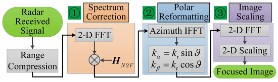
Figure 4. The flowchart of extended polar format algorithm (EPFA) for near-field ISAR imaging.

2.5. CSAR Spectrum Analysis Based on TFRSA and EPFA-Based CSAR Imaging Method

In the CSAR imaging geometry, which is illustrated in Figure 5, the radar moves along a circular trajectory and continuously observes the same scene. This leads to a much large observation angle, which could produce ultrahigh resolution radar image of the scene. The CASR imaging geometry is equivalent to the geometry of the near-field turntable ISAR without consideration of the height of the trajectory. This means we can apply the EPFA to the CSAR imaging with some additional compensation processing. According to the geometry in Figure 5, the slant range of the i-th scatterer can be expressed by

$$\begin{array}{cc}\hfill R_i^{CSAR}\left(\theta ,H\right)& =\sqrt{{\left(r_{0}cos\gamma cos\theta -y_i\right)}^2+{\left(r_{0}cos\gamma sin\theta -x_i\right)}^2+H^2}\hfill \\ & \approx \sqrt{{\left(r_0-x_{i}sin\theta cos\gamma -y_{i}cos\theta cos\gamma \right)}^2+{\left(x_{i}cos\theta cos\gamma -y_{i}sin\theta cos\gamma \right)}^2}\hfill \\ & +\frac{\left(x_i^2+y_i^2\right){sin}^2\gamma }{\sqrt{{\left(r_0-y_{i}cos\gamma \right)}^2+x_i^2{cos}^2\gamma }}\hfill \end{array},$$

(48)

where $\theta$ and $\gamma$ denote the rotational angle of the radar along the circular orbit and the elevation angle of the orbit, respectively, which are illustrated in Figure 5. $r_0$ stands for the distance between the radar and the scene center and H signifies the height of the orbit, which can be expressed by $H=r_{0}sin\gamma$. Observing the approximation result of Equation (48) and comparing it with Equation (19), the CSAR slant range has the same form as the near-field ISAR slant range without consideration of the constant error. Because the constant error does not influence the signal spectrum, we can still apply the EPFA to CSAR to obtain the equivalent far-field signal. However, the error would influence the polar reformatting result, which would cause distortion and defocusing to the final image.

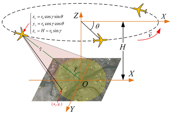
Figure 5. Imaging geometry of CSAR.

Substituting Equation (48) into the signal model of Equation (3), the received CSAR signal after down conversion and range compression can be expressed as

$$\begin{array}{cc}\hfill s\left(k_r,\theta \right)& =\sum _{i=1}^K{A}_{i}rect\left[\frac{k_r}{\mathsf{\Delta }{k}_r}\right]exp\left(-j{k}_r\sqrt{{\left(r_0-y_{i}cos\theta cos\gamma \right)}^2+{\left(r_0-x_{i}sin\theta cos\gamma \right)}^2}\right)\hfill \\ & \times exp\left(-j{k}_r\frac{\left(x_i^2+y_i^2\right){sin}^2\gamma }{\sqrt{{\left(r_0-y_{i}cos\gamma \right)}^2+x_i^2{cos}^2\gamma }}\right)\hfill \end{array},$$

(49)

Performing EPFA to Equation (49), we can obtain

$$\begin{array}{c}s\left(k_{\beta },k_{\alpha }\right)\hfill \\ =\sum _{i=1}^K{A}_{i}rect\left[\frac{k_{\beta }-k_{\beta }^{ic}}{\mathsf{\Delta }{k}_{\beta }^i}\right]rect\left[\frac{k_{\alpha }-k_{\alpha }^{ic}}{\mathsf{\Delta }{k}_{\alpha }^i}\right]exp\left[j\left(k_{\alpha }{x}_{i}cos\gamma +k_{\beta }{y}_{i}cos\gamma \right)\right]\hfill \\ \times exp\left(-j\sqrt{k_{\alpha }^2+k_{\beta }^2}\frac{\left(x_i^2+y_i^2\right){sin}^2\gamma }{\sqrt{{\left(r_0-y_{i}cos\gamma \right)}^2+x_i^2{cos}^2\gamma }}\right)\hfill \\ \approx \sum _{i=1}^K{A}_{i}rect\left[\frac{k_{\beta }-k_{\beta }^{ic}}{\mathsf{\Delta }{k}_{\beta }^i}\right]rect\left[\frac{k_{\alpha }-k_{\alpha }^{ic}}{\mathsf{\Delta }{k}_{\alpha }^i}\right]exp\left[j\left(k_{\alpha }{x}_{i}cos\gamma +k_{\beta }{y}_{i}cos\gamma \right)\right]exp\left[j\left({\phi }_{e1}+{\phi }_{e2}\right)\right]\hfill \end{array},$$

(50)

with

$${\phi }_{e1}=-k_{\beta }\frac{x_i^2{sin}^2\gamma }{\sqrt{r_0^2+x_i^2{cos}^2\gamma }},$$

(51)

$${\phi }_{e2}=-\sqrt{k_{\alpha }^2+k_{\beta c}^2}\frac{y_i^2{sin}^2\gamma }{r_0-y_{i}cos\gamma },$$

(52)

where ${\phi }_{e1}$ and ${\phi }_{e2}$ signify the decomposed range profile error and phase error, which would cause distortion and defocusing, respectively. $k_{\beta c}$ stands for the center of the range wavenumber $k_{\beta }$.

In order to generate the focused image without distortion, we first compensate the range profile error. Transforming Equation (50) to range wavenumber and azimuth position domains by applying azimuth FT, we obtain

$$s\left(k_{\beta },x\right)=\sum _{i=1}^K{A}_{i}rect\left[\frac{k_{\beta }-k_{\beta }^{ic}}{\mathsf{\Delta }{k}_{\beta }^i}\right]sinc\left[\frac{x-x_{i}cos\gamma }{\eta 2\pi /\mathsf{\Delta }{k}_{\alpha }^i }\right]exp\left[j{k}_{\beta }{y}_{i}cos\gamma \right]exp\left[j{\phi }_{e1}\right],$$

(53)

where $\eta$ stands for the azimuth main-lobe expansion factor caused by the phase error ${\phi }_{e2}$. Observing the sinc function term of Equation (53) reveals that the azimuth positions of scatterers are scaled by the factor $cos\gamma$. We construct the range profile compensation functions in the range wavenumber and azimuth position domain by

$$H_{EC1}\left(k_{\beta },x_n\right)=exp\left(j{k}_{\beta }\frac{x_n^2{sin}^2\gamma /{cos}^2\gamma }{\sqrt{r_0^2+x_n^2}}\right),$$

(54)

with

$$x_n=\frac{1}{cos\gamma }\left(n-\frac{N_a}{2}\right)\frac{2\pi }{\mathsf{\Delta }{k}_{\alpha }},n=1,2,\dots ,N_a,$$

(55)

where $x_n$ denotes the real X-coordinate of the n-th azimuth pixel, $N_a$ signifies the number of the pixels in azimuth dimension, and the term $2\pi /\mathsf{\Delta }{k}_{\alpha }$ stands for the size of the image pixel in azimuth dimension.

After compensating the range profile error, the signal is transformed into the range position and azimuth wavenumber domains, and it yields

$$\begin{array}{cc}\hfill s\left(y,k_{\alpha }\right)& =\sum _{i=1}^K{A}_{i}sinc\left[\frac{y-\left(y_{i}cos\gamma +y_i^2{sin}^2\gamma /\left(R_0-y_{i}cos\gamma \right)\right)}{2\pi /\mathsf{\Delta }{k}_{\beta }^i}\right]rect\left[\frac{k_{\alpha }-k_{\alpha }^{ic}}{\mathsf{\Delta }{k}_{\alpha }^i}\right]\hfill \\ & \times exp\left[j{k}_{\alpha }{x}_{i}cos\gamma \right]exp\left[j{\phi }_{e2}\right],\hfill \end{array}$$

(56)

From Equation (56), we can find that the focus positions of scatterers in range dimension are modulated by a complex function, which is given by

$${\widehat{y}}_i=M\left(y_i\right)=y_{i}cos\gamma +y_i^2{sin}^2\gamma /\left(R_0-y_{i}cos\gamma \right) ,$$

(57)

where ${\widehat{y}}_i$ stands for the real focus position and $M\left( \right)$ signifies the focus position modulation function. We can solve the real Y-coordinates of image pixels by using the inverse function of $M\left( \right)$, and it yields

$$y_m=M^{-1}\left({\widehat{y}}_m\right),$$

(58)

with

$${\widehat{y}}_m=\left(m-\frac{N_r}{2}\right)\frac{2\pi }{\mathsf{\Delta }{k}_{\beta }},m=1,2,\dots ,N_r,$$

(59)

where ${\widehat{y}}_m$ denotes the focus position of the m-th range pixel and $y_m$ depicts the real Y-coordinate of the m-th range pixel. Thus, the phase error compensation function can be constructed by

$$H_{EC2}\left(k_{\alpha },y_m\right)=exp\left(j\sqrt{k_{\alpha }^2+k_{\beta c}^2}\frac{y_m^2{sin}^2\gamma }{r_0-y_{m}cos\gamma }\right),$$

(60)

After compensating the phase error, the signal can be expressed as

$$s\left(y,k_{\alpha }\right)=\sum _{i=1}^K{A}_{i}sinc\left[\frac{y-\left(y_{i}cos\gamma +y_i^2{sin}^2\gamma /\left(R_0-y_{i}cos\gamma \right) \right)}{2\pi /\mathsf{\Delta }{k}_{\beta }^i }\right]rect\left[\frac{k_{\alpha }-k_{\alpha }^{ic}}{\mathsf{\Delta }{k}_{\alpha }^i}\right]exp\left[j{k}_{\alpha }{x}_{i}cos\gamma \right],$$

(61)

Finally, the focused CSAR imaging result can be obtained by applying the azimuth FT to Equation (61), and it yields

$$I\left(x,y\right)=\sum _{i=1}^K{A}_{i}sinc\left[\frac{y-\left(y_{i}cos\gamma +y_i^2{sin}^2\gamma /\left(R_0-y_{i}cos\gamma \right) \right)}{2\pi /\mathsf{\Delta }{k}_{\beta }^i }\right]sinc\left[\frac{x-x_{i}cos\gamma }{2\pi /\mathsf{\Delta }{k}_{\alpha }^i}\right],$$

(62)

Besides, the vectors $x_n$ and $y_m$ can be used to scale the image in azimuth and range dimensions, respectively. Finally, the flowchart of the EPFA-based CSAR imaging method is illustrated in Figure 6.

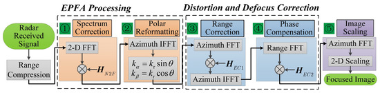
Figure 6. Flowchart of EPFA-based CSAR imaging method.

3. Results

To evaluate the performance of the proposed TFRSA and EPFA, we use both simulated and real data. Results achieved by the proposed EPFA are compared with those obtained by traditional PFA and BPA. Apart from comparing the visual images, the entropy, impulse response width (IRW), and peak side lobe ratio (PSLR) of the final focused images are measured to assess image qualities and the running times are measured to assess their efficiencies. Because the proposed method is not revolved in parameters estimation, the performance comparison between the proposed methods and other methods under various SNR conditions will not have a much difference.

3.1. Simulations

3.1.1. Simulation for Near-Field ISAR Imaging

The simulated radar parameters for near-field ISAR are listed in Table 1. The target point model of the airplane is shown in Figure 7a and the distance between radar and target is 10 m. The imaging results of different algorithms are presented in Figure 7b–d, which correspond to the PFA, BPA, and EPFA, respectively. Observing Figure 7b reveals that the imaging result of PFA is severely distorted and defocused when it is compared with the target point model in Figure 7a, whereas the BPA and EPFA in Figure 7c,d both show perfect airplane shape without obvious defocusing. It is worth mentioning that because the BPA is an accurate time-domain imaging algorithm, it is used as reference in this paper. In this simulation, the running times of BPA and PFA are 141.89 s and 11.29 s, respectively. For EPFA, we use the nonuniform FFT (NUFFT) [30] to speed up the polar reformatting operation and its running time is 2.22 s. It is clear that EPFA is highly efficient and is very suitable for real-time applications.

Table 1. Near-field ISAR imaging simulation parameters.

Near-Field ISAR Simulation Parameters	Values	Near-Field ISAR Simulation Parameters	Values
Bandwidth B	1 GHz	Pulse Width $T_p$	1 μs
Sampling Frequency $F_s$	1.1 GHz	Carrier Frequency $f_c$	10 GHz
Pulse Repeat Frequency $f_{PRF}$	500 Hz	Rotational Angle $\mathsf{\Delta }\theta$	$47°$

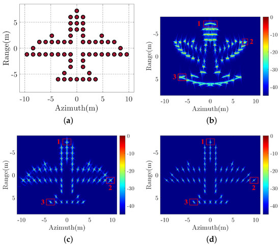
Figure 7. Target point model and imaging results. (a) Airplane point model. (b) ISAR Imaging result of polar format algorithm (PFA). (c) ISAR Imaging result of back-projection algorithm (BPA). (d) ISAR Imaging result of EPFA.

In order to have a more detailed comparison, the contour maps of three edge points, which are located at the head, right-wing, and left tail of the airplane, are plotted in Figure 8. Results from different algorithms are presented in the different columns, beginning with the first column for PFA, then the second column for BPA, and then the third column for EPFA. Different points are demonstrated in the different rows. It can be observed that, the contour maps of PFA are defocused severely, whereas the contour maps of EPFA are similar to those of BPA, that all of them have elliptical main-lobes and they are well separated from their side-lobes. The azimuth slices of the contour maps are also plotted in Figure 9, from which we can find the main-lobes of EPFA are narrower than those of PFA and similar to those of BPA. This signifies that EPFA has high accuracy in near-filed ISAR imaging.

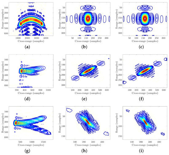
Figure 8. Contour maps of the selected points in the imaging results. (a–c) Contour map of point 1 in the PFA result. (d–f) Contour map of point 1 in the BPA result. (g–i) Contour map of point 1 in the EPFA result.

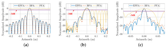
Figure 9. Azimuth slices of the selected points by different imaging algorithms. (a) Azimuth slices of point 1. (b) Azimuth slices of point 2. (c) Azimuth slices of point 3.

In order to make a quantitative comparison, some parameters, which can evaluate the image quality, are calculated and listed in Table 2. The entropy [31,32,33] is a statistical measure of randomness that can be used to characterize the focus performance of the radar image and it is defined by

$$En=-\sum _{i=1}^{MN}\left(p_{i}log{p}_i\right),$$

(63)

with

$$p_i={\left|I_i\right|}^2/\sum _{i=1}^{MN}{\left|I_i\right|}^2,$$

(64)

where $I_i$ and $p_i$ denote the value and the normalized power of the i-th element of the image. The smaller the entropy, the higher the image quality. The impulse response width (IRW) and the peak side lobe ratio (PLSR) of the image slice are used to measure the focusing performance. From Table 2 we can find that the entropies, IRWs and PLSRs of EPFA are smaller than PFA, whereas they are similar to those of BPA. Thus, the simulation result validate the effectiveness of the proposed EPFA.

Table 2. Image performance parameters comparison of near-field ISAR simulation.

Algorithms	Entropy	IRW (m)			PLSR (dB)			Time (s)
		P1	P2	P3	P1	P2	P3
PFA	11.29	Null	0.19	0.058	$-0.54$	$-2.97$	$-3.61$	11.29
BPA	9.29	0.027	0.045	0.013	$-13.05$	$-14.58$	$-7.68$	141.88
EPFA	9.41	0.027	0.047	0.013	$-12.94$	$-14.51$	$-10.72$	2.22

3.1.2. Simulation for CSAR Imaging

The simulated radar parameters for CSAR are listed in Table 3. The scene of a 11 × 11 points array is shown in Figure 10a and the distance from radar to the center of the scene is 1100 m. The imaging results of different algorithms are shown in Figure 10b–d, which corresponding to the PFA, BPA, and the proposed method, respectively. Observing Figure 10b reveals that the imaging result of PFA is obviously distorted with a trapezoid shape, whereas the imaging results of BPA and the proposed method both show the standard square shape in Figure 10c,d. Besides, the running time for the proposed method is 8.78 s by using the NUFFT acceleration, whereas they are 3242.70 s and 81.96 s for BPA and PFA, respectively. We can find there is a large improvement in the efficiency using the proposed method.

Table 3. CSAR simulation parameters.

CSAR Simulation Parameters	Values	CSAR Simulation Parameters	Values
Bandwidth B	500 MHz	Pulse Width $T_p$	600 μs
Sampling Frequency $F_s$	600 MHz	Carrier Frequency $f_c$	10 GHz
Pulse Repeat Frequency $f_{PRF}$	8000 Hz	Rotational Angle $\mathsf{\Delta }\theta$	$14.67°$
Reference Range $r_0$	1100 m	Trajectory Height H	214.60 m

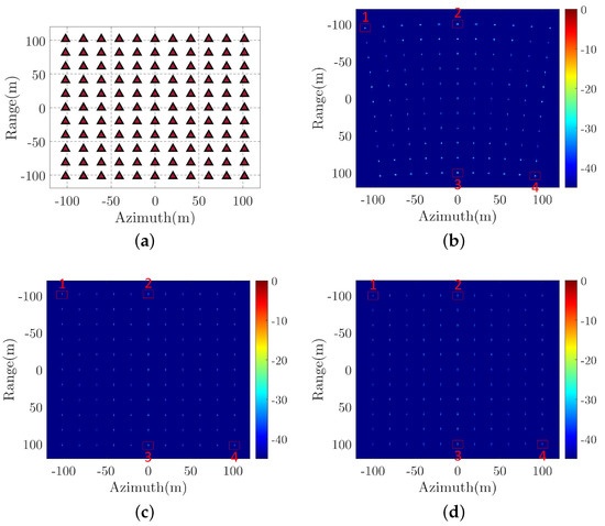
Figure 10. Target point model and imaging results. (a) Point array Scene. (b) CSAR Imaging result of PFA. (c) CSAR Imaging result of BPA. (d) CSAR Imaging result of proposed method.

The contour maps of four edge points are plotted to make a detailed comparison, which are shown in Figure 11. Different methods are presented in the different columns, beginning with the first column for PFA, then the second column for BPA, and then the third column for the proposed method. Different points are demonstrated in the different rows. Observing these contour maps, for PFA, they are defocused severely and their main lobes are connected with the side-lobes, whereas for the proposed method, they are similar to those of BPA, all of them have elliptical main lobes and separated side-lobes. The azimuth slices of the contour maps are also illustrated in Figure 12, which shows the proposed method has similar focus ability to the BPA.

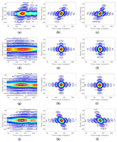
Figure 11. Contour maps of the selected points. (a–c) Contour map of point 1 by different imaging algorithms. (d–f) Contour map of point 2 by different imaging algorithms. (g–i) Contour map of point 3 by different imaging algorithms. (j–l) Contour map of point 4 by different imaging algorithms.

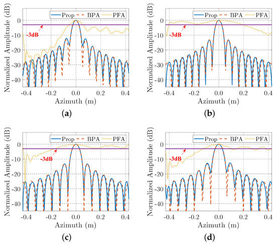
Figure 12. Azimuth slices of the selected points by different imaging algorithms. (a) Azimuth slices of point 1. (b) Azimuth slices of point 2. (c) Azimuth slices of point 3. (d) Azimuth slices of point 4.

In order to make a quantitative comparison, the IRWs and PLSRs of the azimuth slices are calculated and listed in Table 4. Besides, the image entropies are also calculated. From Table 4, we can find that the entropy, IRW, and PLSR of EPFA are similar to those of BPA while they are smaller than those of PFA. The simulation results validate the effectiveness of the proposed EPFA-based CSAR imaging method.

Table 4. Image performance parameters comparison of CSAR simulation.

Methods	Entropy	IRW (m)				PLSR (dB)				Time (s)
		P1	P2	P3	P4	P1	P2	P3	P4
PFA	9.72	0.11	0.40	0.35	0.30	$-4.93$	$-0.61$	$-0.23$	$-0.52$	81.96
BPA	8.21	0.046	0.046	0.059	0.059	$-13.21$	$-13.16$	$-13.27$	$-13.21$	3242.70
Proposed	8.22	0.046	0.046	0.059	0.059	$-12.17$	$-13.23$	$-13.27$	$-12.59$	3.24

3.2. Real Data Processing Results

Real near-field ISAR data are collected in a microwave anechoic chamber, in which an aircraft model target is placed on the turntable model as shown in Figure 13a. The radar is fixed, and the height of radar is set a little bit higher than the turntable surface. The horizontal distance between the radar and the turntable surface is 7 m. The rotational angle of turntable can be precisely controlled, and it is changed discretely with step of 0.2 degree. The radar transmits and receives signal at every discrete rotational angle. The parameters of the radar are listed in the Table 5.

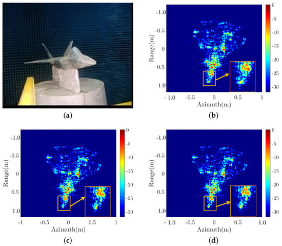
Figure 13. Target point model and imaging results. (a) Real experiment scene. (b) Real data ISAR Imaging result of PFA. (c) Real data ISAR Imaging result of BPA. (d) Real data ISAR Imaging result of EPFA.

Table 5. Near-field ISAR radar parameters.

Radar Parameters	Values	Radar Parameters	Values
Bandwidth B	4 GHz	Carrier Frequency $f_c$	10 GHz
Reference Range $R_0$	7 m	Rotational Angle $\mathsf{\Delta }\theta$	$40°$

The imaging results based on the real data processed by different algorithms are illustrated in Figure 13b–d, which corresponding to the PFA, BPA, and EPFA, respectively. Observing Figure 13b, we can find that the head of the aircraft, which is marked with a rectangular, shows an expanded main-lobe for PFA, whereas in Figure 13c,d, their aircraft head parts show more focused main lobes. The contour maps of the aircraft’s head are plotted in Figure 14, in which the main lobe of PFA is of an oval shape whereas they are round for BPA and EPFA. The azimuth slices of the contour maps are plotted in Figure 15 for further comparison, in which the main lobe of the PFA is obviously wider than that of BPA and PFA. The performance parameters of image entropy, IRW, PLSR, and running time are calculated and listed in Table 6 for a quantitative comparison. We can find that the results of EPFA are similar to the results of BPA, while they are smaller than those of PFA. In addition, the running time for EFPA is much smaller than BPA. The real data processing result validate the effectiveness of the proposed EPFA.

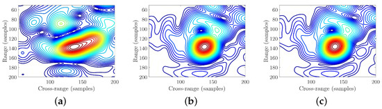
Figure 14. Contour maps of the aircraft’s head. (a) Contour map of the aircraft’s head by PFA. (b) Contour map of the aircraft’s head by BPA. (c) Contour map of the aircraft’s head by EPFA.

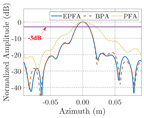
Figure 15. Azimuth slices of the aircraft’s head by different algorithms.

Table 6. Image performance parameters comparison of near-field ISAR real data processing.

Methods	Entropy	IRW (m)	PLSR (dB)	Time (s)
PFA	9.75	0.040	$-12.25$	0.45
BPA	9.70	0.019	$-12.63$	1.12
EPFA	9.69	0.019	$-13.02$	0.04

4. Discussion

PFA is one of the common imaging algorithms for SAR and ISAR because of its simplicity and efficiency. However, due to the plane wave assumption of PFA, it would produce large slant range error for near-field ISAR and wide scene SAR, which would generate range profiles migration and azimuth phase error, and thus cause the image to be distorted and defocused. Because the BPA constructs user-defined grids, the accurate slant range of every grid can be calculated by the known trajectory information. Then, radar returns can be accumulated coherently for every grid by using this accurate slant range. BPA is an accurate imaging algorithm for all modes of SAR and ISAR, so it would produce focused image without distortion. The drawback of BPA is its large computation cost. On the other hand, according to the introduction of the proposed TFRSA in the Section 2.2, the influence of the envelopes of the scatterer’s returns can be ignored. This approximation is applicable and often used in radar signal processing because the envelope is usually a low-frequency and narrow bandwidth signal. Thus, the proposed TFRSA-based EPFA has high accuracy in radar imaging and generates comparably high image quality to BPA.

For the future research, we will focus on the possibility of applying the TFRSA to more applications and consider the influence of the motion error in the realistic environments. Now, we are trying to apply the proposed method to the helical SAR(HSAR)2D imaging, HSAR and tomographic CSAR 3D imaging, and the primary results is prove that the proposed method is valid to these applications.

5. Conclusions

In this paper, a time-frequency reversion-based spectrum analysis (TFRSA) method is proposed, which utilizes the relationship of the Fourier pairs and their corresponding signal phase. Based on this method, the spectrum of the linear trajectory SAR is analyzed. The derived spectrum expression is shown to be the same as the result of the POSP. In addition, the TFRSA is also applied to the near-field ISAR, which the POSP cannot be applied to. The spectrum expression of near-field ISAR is derived and it is compared with the far-field ISAR spectrum expression. The spectrum difference is found to be position-independent. Based on this finding, an extended PFA is proposed to solve the distortion and defocusing problems caused by traditional ISAR imaging algorithms. Because the CSAR has similar imaging geometry to the near-field ISAR, its spectrum is also derived by TFRSA and an EPFA-based imaging method is proposed to improve the imaging efficiency. Simulations and real data processing results validate the effectiveness of the proposed TFRSA, EPFA, and EPFA-based CSAR imaging method.

References

- Wehner, D.R. High Resolution Radar; Artech House: Norwood, MA, USA, 1987. [Google Scholar]
- Mensa, D.L. High Resolution Radar Imaging; Artech House: Norwood, MA, USA, 1981. [Google Scholar]
- Cumming, I.; Wong, F. Digital Processing of Synthetic Aperture Radar Data: Algorithms and Implementation; Artech House: Norwood, MA, USA, 2005. [Google Scholar]
- Chen, C.C.; Andrews, H.C. Target-motion-induced radar imaging. IEEE Trans. Aerosp. Electron. Syst. 1980, 2–14. [Google Scholar] [CrossRef]
- Chen, V.C. Inverse Synthetic Aperture Radar Imaging: Principles, Algorithms and Applications; Institution of Engineering and Technology: London, UK, 2014. [Google Scholar]
- Chen, V.C.; Ling, H. Time-Frequency Transforms for Radar Imaging and Signal Analysis; Artech House: Norwood, MA, USA, 2002. [Google Scholar]
- Yao, J. Microwave photonics. J. Light. Technol. 2009, 27, 314–335. [Google Scholar] [CrossRef]
- McKinney, J.D. Photonics illuminates the future of radar. Nature 2014, 507, 310–312. [Google Scholar] [CrossRef] [PubMed]
- Capmany, J.; Novak, D. Microwave photonics combines two worlds. Nat. Photonics 2007, 1, 319–330. [Google Scholar] [CrossRef]
- Gao, Y.; Xing, M.; Zhang, Z.; Guo, L. Ultrahigh Range Resolution ISAR Processing by Using KT–TCS Algorithm. IEEE Sens. J. 2018, 18, 8311–8317. [Google Scholar] [CrossRef]
- Yang, L.; Xing, M.; Zhang, L.; Sun, G.; Gao, Y.; Zhang, Z.; Bao, Z. Integration of Rotation Estimation and High-Order Compensation for Ultrahigh-Resolution Microwave Photonic ISAR Imagery. IEEE Trans. Geosci. Remote. Sens. 2020, 1–21. [Google Scholar] [CrossRef]
- Bleistein, N.; Handelsman, R.A. Asymptotic Expansions of Integrals; Courier Corporation: North Chelmsford, MA, USA, 1986. [Google Scholar]
- Li, J.; Zhang, S.; Chang, J. Bistatic forward-looking SAR imaging based on two-dimensional principle of stationary phase. In Proceedings of the 2012 International Workshop on Microwave and Millimeter Wave Circuits and System Technology, Chengdu, China, 19–20 April 2012; pp. 1–4. [Google Scholar]
- Andre, S.; Ruben, R. Analysis of scattering arrays using the principle of stationary phase. In Proceedings of the 1964 Antennas and Propagation Society International Symposium, Long Island, NY, USA, 21–24 September 1964; Volume 2, pp. 19–23. [Google Scholar]
- Chassande-Mottin, E.; Flandrin, P. On the stationary phase approximation of chirp spectra. In Proceedings of the IEEE-SP International Symposium on Time-Frequency and Time-Scale Analysis (Cat. No. 98TH8380), Pittsburgh, PA, USA, 9 October 1998; pp. 117–120. [Google Scholar]
- Yang, Z.; Xing, M.; Zhang, Y.D.; Sun, G.; Bao, Z. Factorised polar-format back-projection algorithm. IET Radar Sonar Navig. 2015, 9, 875–880. [Google Scholar] [CrossRef]
- Li, H.; Zhang, L.; Xing, M.; Bao, Z. Expediting back-projection algorithm for circular SAR imaging. Electron. Lett. 2015, 51, 785–787. [Google Scholar] [CrossRef]
- Mengdao, X.; Renbiao, W.; Jinqiao, L.; Zheng, B. Migration through resolution cell compensation in ISAR imaging. IEEE Geosci. Remote. Sens. Lett. 2004, 1, 141–144. [Google Scholar] [CrossRef]
- Zhang, L.; Sheng, J.-l.; Duan, J.; Xing, M.-d.; Qiao, Z.-j.; Bao, Z. Translational motion compensation for ISAR imaging under low SNR by minimum entropy. EURASIP J. Adv. Signal Process. 2013, 2013, 33. [Google Scholar] [CrossRef]
- Li, D.; Zhan, M.; Liu, H.; Liao, Y.; Liao, G. A robust translational motion compensation method for ISAR imaging based on keystone transform and fractional Fourier transform under low SNR environment. IEEE Trans. Aerosp. Electron. Syst. 2017, 53, 2140–2156. [Google Scholar] [CrossRef]
- Ji, Z.; Zhu, X. Application of DBF in 77 GHz Automotive Millimeter-wave Radar. In IOP Conference Series: Materials Science and Engineering; IOP Publishing: Bristol, UK, 2019; Volume 490, p. 072066. [Google Scholar] [CrossRef]
- Keziah, J.; Muthukumaran, N. Design of K Band Transmitting Antenna for Harbor Surveillance Radar Application. Int. J. Appl. Electr. Electron. Eng. 2016, 2, 16–20. [Google Scholar]
- Turin, F.; Pastina, D.; Lombardo, P.; Corucci, L. ISAR imaging of ground targets with an X-band FMCW Radar system for airport surveillance. In Proceedings of the IEEE 2014 15th International Radar Symposium (IRS), Gdansk, Poland, 16–18 June 2014; pp. 1–5. [Google Scholar] [CrossRef]
- Amin, M.G. Spectral decomposition of time-frequency distribution kernels. IEEE Trans. Signal Process. 1994, 42, 1156–1165. [Google Scholar] [CrossRef]
- Cohen, L. Time-frequency distributions-a review. Proc. IEEE 1989, 77, 941–981. [Google Scholar] [CrossRef]
- Xu, G.; Xing, M.; Zhang, L.; Duan, J.; Chen, Q.; Bao, Z. Sparse Apertures ISAR Imaging and Scaling for Maneuvering Targets. IEEE J. Sel. Top. Appl. Earth Obs. Remote. Sens. 2014, 7, 2942–2956. [Google Scholar] [CrossRef]
- Bailey, D.H.; Swarztrauber, P.N. The fractional Fourier transform and applications. SIAM Rev. 1991, 33, 389–404. [Google Scholar] [CrossRef]
- Ozaktas, H.M.; Kutay, M.A. The fractional fourier transform. In Proceedings of the 2001 European Control Conference (ECC), Porto, Portugal, 4–7 September 2001; pp. 1477–1483. [Google Scholar]
- Rafaely, B. Plane-wave decomposition of the sound field on a sphere by spherical convolution. J. Acoust. Soc. Am. 2004, 116, 2149–2157. [Google Scholar] [CrossRef]
- Greengard, L.; Lee, J.Y. Accelerating the nonuniform fast Fourier transform. SIAM Rev. 2004, 46, 443–454. [Google Scholar] [CrossRef]
- Flores, B.C.; Ugarte, A.; Kreinovich, V. Choice of an entropy-like function for range-Doppler processing. In Proceedings of the Automatic Object Recognition III, International Society for Optics and Photonics, Orlando, FL, USA, 11–16 April 1993; Volume 1960, pp. 47–56. [Google Scholar]
- Xi, L.; Guosui, L.; Ni, J. Autofocusing of ISAR images based on entropy minimization. IEEE Trans. Aerosp. Electron. Syst. 1999, 35, 1240–1252. [Google Scholar] [CrossRef]
- Kragh, T.J.; Kharbouch, A.A. Monotonic iterative algorithm for minimum-entropy autofocus. In Proceedings of the Adaptive Sensor Array Processing (ASAP) Workshop, Lexington, MA, USA, 6–7 June 2006; Volume 40, pp. 1147–1159. [Google Scholar]
Publisher’s Note: MDPI stays neutral with regard to jurisdictional claims in published maps and institutional affiliations. |
© 2021 by the authors. Licensee MDPI, Basel, Switzerland. This article is an open access article distributed under the terms and conditions of the Creative Commons Attribution (CC BY) license (http://creativecommons.org/licenses/by/4.0/).