Article

3D Reconstruction of Coastal Cliffs from Fixed-Wing and Multi-Rotor UAS: Impact of SfM-MVS Processing Parameters, Image Redundancy and Acquisition Geometry

by
Gil Gonçalves
1,2,*,
Diogo Gonçalves
2,3,
Álvaro Gómez-Gutiérrez
4,
Umberto Andriolo
2 and
Juan Antonio Pérez-Alvárez
5
1
Department of Mathematics, University of Coimbra, 3001-501 Coimbra, Portugal
2
Institute for Systems Engineering and Computers at Coimbra (INESC-Coimbra), DEEC, 3030-290 Coimbra, Portugal
3
Department of Civil Engineering, University of Coimbra, 3030-788 Coimbra, Portugal
4
Research Institute for Sustainable Territorial Development (INTERRA), University of Extremadura, Avda. de la Universidad s/n, 10071 Cáceres, Spain
5
Graphic Expression Department, University Centre of Merida (CUM), University of Extremadura, Merida, 06800 Badajoz, Spain
*
Author to whom correspondence should be addressed.
Remote Sens. 2021, 13(6), 1222; https://doi.org/10.3390/rs13061222
Submission received: 3 February 2021 / Revised: 7 March 2021 / Accepted: 20 March 2021 / Published: 23 March 2021
(This article belongs to the Special Issue Advances in Remote Sensing in Coastal Geomorphology)

Abstract

:
Monitoring the dynamics of coastal cliffs is fundamental for the safety of communities, buildings, utilities, and infrastructures located near the coastline. Structure-from-Motion and Multi View Stereo (SfM-MVS) photogrammetry based on Unmanned Aerial Systems (UAS) is a flexible and cost-effective surveying technique for generating a dense 3D point cloud of the whole cliff face (from bottom to top), with high spatial and temporal resolution. In this paper, in order to generate a reproducible, reliable, precise, accurate, and dense point cloud of the cliff face, a comprehensive analysis of the SfM-MVS processing parameters, image redundancy and acquisition geometry was performed. Using two different UAS, a fixed-wing and a multi-rotor, two flight missions were executed with the aim of reconstructing the geometry of an almost vertical cliff located at the central Portuguese coast. The results indicated that optimizing the processing parameters of Agisoft Metashape can improve the 3D accuracy of the point cloud up to 2 cm. Regarding the image acquisition geometry, the high off-nadir (90°) dataset taken by the multi-rotor generated a denser and more accurate point cloud, with lesser data gaps, than that generated by the low off-nadir dataset (3°) taken by the fixed wing. Yet, it was found that reducing properly the high overlap of the image dataset acquired by the multi-rotor drone permits to get an optimal image dataset, allowing to speed up the processing time without compromising the accuracy and density of the generated point cloud. The analysis and results presented in this paper improve the knowledge required for the 3D reconstruction of coastal cliffs by UAS, providing new insights into the technical aspects needed for optimizing the monitoring surveys.

Graphical Abstract

1. Introduction

Coastal cliffs are specific coastal landforms characterized by steep rocky walls, which are present on about 52% of the global shoreline [1,2]. Their complex face topography, with ledge crevices and overhangs, is the result of geological, physical and environmental processes interplaying at the coast. The erosional processes of cliffs are mainly caused by the notching at their base due to wave forcing, and/or by the collapse of the cliff face due to the combination of atmospheric and marine processes [2]. The current sea level rise in the actual climatic change scenario is further intensifying the erosional processes [1].
It is fundamental to monitor the coastal cliffs face stability and to measure its variation, as coastal cliffs provide habitat to flora and fauna [3], their collapse can cause injuries and fatalities [4], and their erosion often threaten coastal communities and infrastructures worldwide [5]. A wide range of methods have been used to monitor coastal cliff erosion, including historic cartographic mapping, aerial photography and photogrammetry, satellite imagery, global navigation satellite systems (GNSS), total stations, airborne and terrestrial laser scanning ([1] and references therein). Nevertheless, in the last decade, the advent of Unmanned Aerial Systems (UAS) has improved the possibility of reconstructing the 3D complex cliff topography [6,7,8,9,10]. In fact, UAS allows to (i) acquire high spatial resolution images at low-cost, (ii) monitor inaccessible areas, overcoming the logistical constraints typical of rock cliff environments, (iii) increase the frequency of the surveys needed to quantify the spatial and temporal cliff response to environmental forcing, which in turn, increases our understanding of rock fall magnitude–frequency relationships.
The 3D reconstruction of a coastal cliff from an image-based UAS survey consists of applying a Structure-from-Motion and Multi View Stereo (SfM-MVS) processing workflow, to generate a dense 3D point cloud, which is then used for building a reliable and detailed 3D model of the cliff surface [11]. Unlike Terrestrial Laser Scanning (TLS) or Airbone Laser Scanning (ALS), SfM-MVS photogrammetry provides a low-cost, flexible, easy to use workflow and does not requires a highly skilled operator for data acquisition and processing [1,12,13].
In the literature, the works devoted to the 3D reconstruction of coastal cliffs from UAS-based topographic surveys focused mainly on the image acquisition and georeferencing strategies, testing the influence of camera angle [8], flight patterns [7] and distribution of ground control points (GCPs) [6,7]. Jaud et al. [8] showed that the use of nadiral images were irrelevant since the final point cloud can have many data gaps (zones without points). Taking the advantage of drones offer to change the imaging angle, the authors studied the impact of this parameter (ranging from nadir to 40° off-nadir) on the accuracy of the 3D reconstruction. Off-nadir aerial coverages were adopted in several UAS-based surveys such as in agroforestry [14,15], urban areas [16,17] and coastal cliffs [7,8,11,18]. In fact, the acquisition geometry of aerial coverages from UAS can be a key factor in the geometric accuracy of the Bundle Block Adjustment (BBA), the density of points in the cloud and the reduction of the occlusions, that is, in reducing the gaps (holes) in point clouds [19]. Combining nadiral and oblique (off-nadir) images optimizes the photogrammetric surveys in stepped areas [20], improves the accuracy of the generated 3D models, but also increases the processing time [21,22]. By placing the 90° angle off nadir for vertical cliffs, a high density of points in the reconstruction is commonly obtained [7].
Several authors (e.g., [8,23,24]) reported that optimal image network configuration, image number, overlap, spatial resolution, and illumination conditions are the key parameters to be considered for accurate tie point detection and for dense point cloud generation. However, the development of methods for quantifying the impact of image acquisition geometry on the quality of the point cloud (i.e., accuracy, density and data gaps) is still lacking. Due to the absence of purely 3D methodologies for analyzing point clouds, it common to reduce its dimensionality to 2D, by projecting the point cloud on a given plane. In [25], this simple approach was used to detect and extract rockfall events of a vertical cliff from time series of TLS-based point clouds. In order to include the third spatial dimension on the analysis of multidimensional point patterns, an intuitive alternative is to voxelize the 3D space. In this context, voxel based techniques have been used for detecting and filling gaps in 3D surface reconstruction [26,27], for semantic segmentation and for classifying point clouds [28], among other applications.
In the last decade, the recent advances in computer vision and the technological development of image sensors and UAS, triggered the appearance of commercial and open source SfM-MVS software packages and popularized the use of photogrammetry by the scientific community [29]. The fully automated “black-box” commercial software packages use simple and optimized interfaces, which in general require the tuning of a few processing parameters, making their adoption easy for inexperienced users. Due to its low-cost, intuitive, easy and user-friendly Graphical User Interface (GUI), Agisoft Metashape (formerly called Photoscan) is perhaps one of the most used SfM-MVS software [12,30,31,32]. For the reconstruction of the 3D scene geometry from a set of overlapping images. Metashape uses a proprietary SfM-MVS workflow, where the technical details about the algorithms are not publicly known [31]. Nonetheless, an important issue that is poorly addressed in the literature is a thorough insight into the impact of the main processing parameters of a given SfM-MVS software package on the accuracy of the 3D reconstruction [33,34].
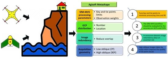
In this context, the objective of this paper was to assess the impact of the main SfM-MVS processing parameters, image redundancy and acquisition geometry of a fixed-wing and a multirotor UAS in the 3D reconstruction of a coastal cliff. By using one of the most used commercial software packages (Agisoft Metashape), a comprehensive analysis of the implemented processing workflow steps was performed, investigating the impact of tuning the default processing parameters and deriving the optimal ones. Adopting the derived optimal processing parameters, the impact of image redundancy in excessive image dataset acquired by multi-rotor was quantified by using two point cloud quality indicators: the point cloud density and data gaps. For the aim, a novel approach based on the voxelization of the point cloud was developed. Finally, the point cloud density and data gaps were used to evaluate the impact of the acquisition geometry of the aerial coverages carried out by each UAS. Overall, the analysis improved the technical knowledge required for the 3D reconstruction of coastal cliff faces by drones.

2. Study Area

Praia do Porto da Calada is an embayed beach at the central Portuguese coast, facing the Atlantic Ocean (Figure 1). The beach is backed by a SW–NE oriented cliff, which belongs geologically to the Mesozoic Lusitanian Basin and shows horizontal sequences of Cretaceous and Jurassic sedimentary rocks. The cliff face has a mean height of 80 m, with a slope gradient of 52°, locally overhanging and devoid of vegetation. At the cliff foot, which is reached by high tides and exposed to storm wave action, rocky debris accumulated with a mean slope gradient of 22°.
The top of the cliff is occupied by residential properties (buildings and courtyards). Below, the sandy subaerial beach is a recreational area with high degree of landslide vulnerability. To improve the safety of the residential and recreational areas an artificial drainage network system was built in order to drain the surface water from the top of the cliff and prevented runoff down the cliff surface [7]. In addition, an artificial flat step (approximately 7 m wide and 200 m long) was built at upper part of the cliff base deposits (mean elevation of 21 m) to stabilize the cliff base and trap the rock falls, protecting also the beach and increasing its usable area (Figure 1b–d).

3. Materials and Methods

With the goal of identifying an optimal SfM-MVS processing workflow that maximizes the precision and accuracy of the dense clouds commonly used in cost-effective monitoring programs of coastal cliffs, the following sections describe (i) the strategies used by each UAS in image acquisition; (ii) a comprehensive analysis of the SfM-MVS processing workflow used in the 3D reconstruction of the cliff surface; (iii) the evaluation criteria used for charactering the quality of the dense point cloud generated in the processing workflow.

3.1. UAS Surveys and GCP Acquisition

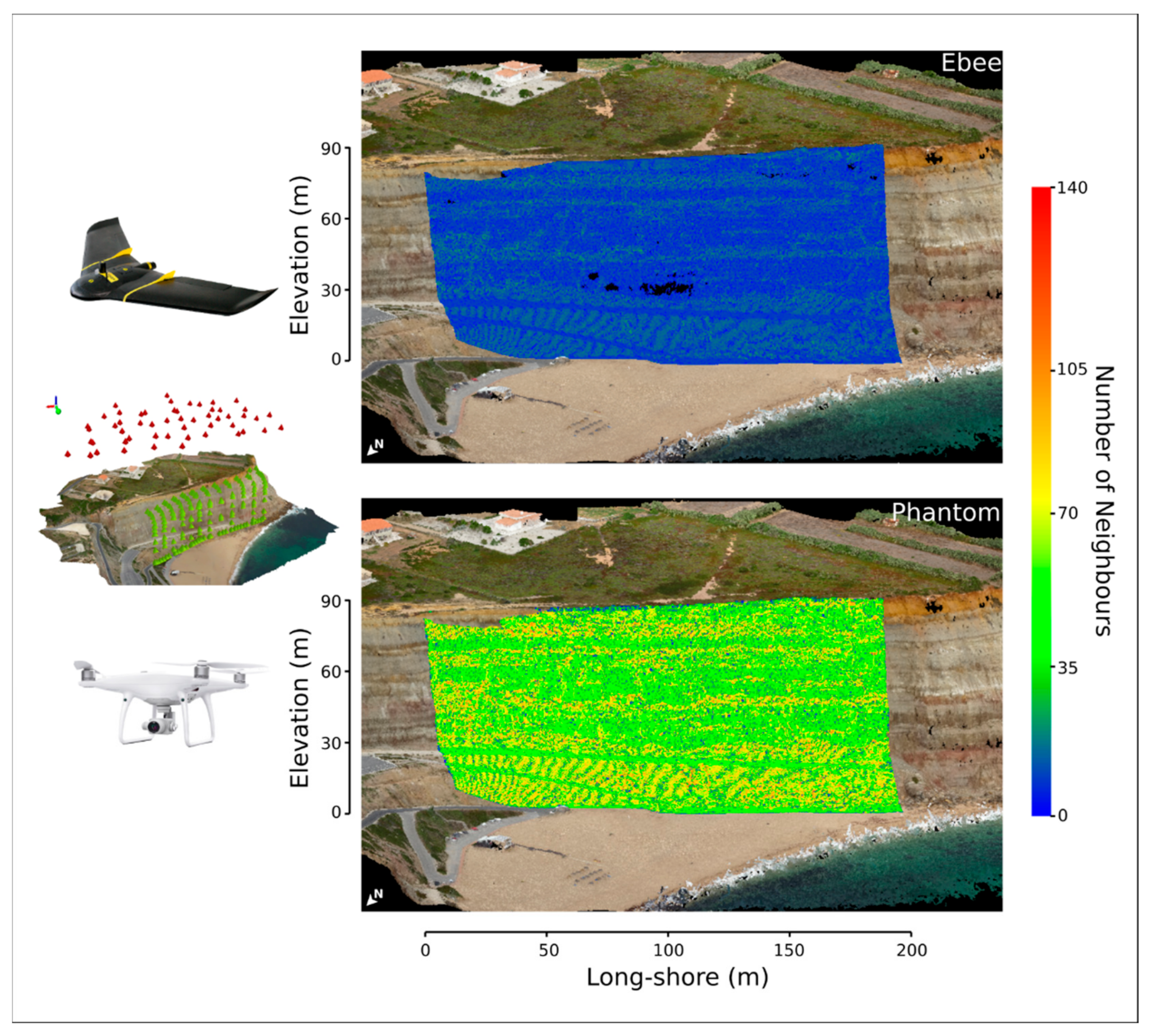
Two flights were performed at the study area on the same date and time, 28 July 2019, under diffusive illumination conditions in order to avoid shadows. Two different UAS platforms were used: the fixed-wing SenseFly® (Cheseaux-sur-Lausanne, Switzerland) Ebee (hereinafter, Ebee), equipped with a Sony WX220 camera (4.45 mm focal length, 18 megapixel) and the multi-rotor DJI® (SZ DJI Technology Co., Shenzhen, China) Phantom 4 Pro (hereinafter, Phantom), equipped with a Sony FC6310 camera (8.80 mm focal length, 20 megapixel). The Ebee does not have a gimbal to point the camera in a given direction. However, the drone can acquire oblique images up to 45° off-nadir, by using a proprietary algorithm that runs onboard on the autopilot and places and orients the drone on the viewing angle defined previously by the user. The Phantom had a three-axis (roll, pitch and yaw) stabilization gimbal and can point the camera in any given viewing angle.
The Ebee flight mission plan was set on eMotion3 software defining a horizontal mapping block of 1.1 ha that was covered with cross flight pattern above the cliff and oblique image acquisition. The front and side overlaps were set to 70% and 65%, respectively. The aircraft flew for 7 min at an average flight altitude of 116 m above the beach (i.e., base of the cliff) and the camera pitch angle was set to 3° for the acquisition of the oblique imagery. Overall, the Ebee collected 53 images with an approximate Ground Sampling Distance (GSD) of 3.3 cm (Figure 2b).
The Phantom flight mission plan was set on the Drone Harmony software [35]. The flight path was set approximately parallel to the cliff, with the camera off-nadir angle (pitch) equal to 90°. The drone flew for 27 min and kept a distance from the cliff face varying from 40 to 60 m. It went up and down on the same line, following vertical stripes and pointing the camera alternatively to the right and to the left of about 10° around the vertical axis (yaw). The front and side overlaps were set to 85% and 70%, respectively. Thus, the vertical stripes were separated from each other by 20 m and two photographs were acquired each time the UAV ascended or descended 6 m (one on the right and one on the left). Finally, to integrate the whole scene, one horizontal stripe was added above the top of the cliff with the camera pointing down (nadir or pitch angle of 0°). The Phantom collected 448 images with a GSD varying from 1.1 to 1.6 cm (Figure 2b). Figure 2c shows the circular distributions of the attitude angles (ω, φ, κ) for the two image datasets. The mean direction (μ) and the resultant vector length (R) are a measure of viewing dispersion (0 means high variability and 1 means low variability) and are commonly used to characterize the angular distributions [36]. Overall, the image data set acquired by the multi-rotor shows a higher variability for the two attitude angles ω and φ, which are the most important for the characterization of the vertical façade plan.
In this work 20 square chessboard targets (50 cm side), used later as Ground Control Points and/or independent Check Points (CHP), were evenly distributed (as much as possible) at three different height levels along the cliff: seven targets on the bottom of the cliff, nine in the intermediate step and four on the top (Figure 2a). These targets were surveyed with a dual-frequency GNSS geodetic receiver (Geomax Zenith 10) in Network Real-Time Kinematic mode (NRTK). The coordinates were only acquired in fix status which ensures positional precision and accuracy at centimeter level [37]. Additional GNSS parameters were simultaneously monitored and analyzed to understand individual target accuracy (Geometric Dilution of Precision or GDOP, number of satellites, Horizontal Standard Deviation (HSDV), and Vertical Standard Deviation (VSDV)).

3.2. 3D Reconstruction from UAS-Based Imagery and SFM-MVS

Generating a georeferenced and dense 3D point cloud from a block of overlapping images with a SfM-MVS method is usually done in five processing steps [12,37,38,39,40]: (A) feature detection; (B) feature matching and geometric validation; (C) sparse 3D reconstruction by SfM; (D) scene geometry georeferencing by GCPs and refinement of the bundle adjustment by including camera self-calibration; (E) dense 3D reconstruction by multi-view stereo dense matching (see Figure 3).
In step A, a Scale Invariant Feature Transform (SIFT) algorithm is commonly used to detect features (or key points) in each image. The key points are invariant to changes in image scale and orientation and partially invariant to photometric distortions and 3D camera view point [41]. The number of key points in each image depends mainly on the texture and resolution [38].
In step B, the key points, characterized by a unique descriptor, are matched in multiple images using, in general, an Approximate Nearest Neighbor (ANN) algorithm. The key point correspondences are then filtered, for each matched image pair, by imposing a geometric epipolar constraint with a RANdom SAmple Consensus (RANSAC) algorithm.
In step C, the geometrically corrected correspondences (i.e., tie points) are used to reconstruct, simultaneously, the 3D geometry of the scene (structure) and the image network geometry (motion) in an iterative bundle adjustment. In this step, the external orientation (extrinsic) parameters (EOP) describing the position and attitude of each image in an arbitrary coordinate system, and the internal camera (intrinsic) parameters (IOP), describing the camera calibration, are also estimated using only the image coordinates of the tie points as observations.
In step D, the sparse 3D point cloud is scaled and georeferenced in the GCP coordinate system, using a 3D similarity transformation (seven parameters) and taken as observations the GCP coordinates measured in general by a dual-frequency GNSS receivers. If a larger number of GCPs are measured and marked on the images where they appear, this additional information can be included in the bundle adjustment to refine the EOP, IOP and the 3D coordinates of the tie points. Using appropriate weights for the measurements of the image (tie points and GCP) and ground (GCP) coordinates, the bundle adjustment is re-run to minimize the reprojection and the georeferencing error.
In step E, the point density of the sparse cloud is increased by several orders of magnitude (in general two or three) by applying a MVS dense matching algorithm. Starting with the sparse cloud, the EOP and IOP (eventually the optimized ones) obtained in step 4, the computational intensive dense matching procedure produces, in the image space, depth maps for each group of images and finally merges them into a global surface estimate of the whole image block [42].
Thorough the above five steps and according the characteristics of the image dataset and the methods and algorithms used in each step, several parameters and thresholds are needed to control and adjust the geometric quality of 3D reconstruction. The different SfM-MVS software packages that are currently used by the geoscience community, whether commercial or open-source, use different names and specific values for the processing parameters. In general, a typical SfM-MVS user performs his processing workflows with the default values recommended by the manufacturer [12,30,31,33,42].

3.3. Impact of the Metashape Processing Parameters

The Metashape processing workflow consists basically in four steps (blue rectangle in Figure 3): (1) determination of the image EOPs and camera IOPs by bundle adjustment (implemented in the GUI function Align Photos); (2) tie points refinement (implemented in Gradual Selection); (3) optimization of the extrinsic and intrinsic camera parameters based on the tie points refinement and eventually on the measured and identified GCPs (implemented in Optimize Cameras); (4) dense reconstruction of the scene geometry (implemented in Build Dense Cloud).
One of the major advantages of Metashape over other SfM-MVS software packages is the possibility of using python scripting Application Program Interface (API) for implementing automated, complex and repetitive processing workflows with minimal user intervention. When comparing the API (light blue rectangles in Figure 3) with the GUI, additional steps are required. First, the Align Photos and Build Dense Cloud steps (step 1 and 4) are performed by two additional functions: matchPhotos and alignCameras for step 1, and buildDepthMaps and buildDenseCloud for step 4. Second, to replicate the Gradual Selection GUI function (step 2) it is necessary to develop a custom API function (in our case the sparse_cloud_filtering).
At each step of the Metashape workflow the user can control and tune some of the preset processing parameters (Table 1). However, in the literature only a few works reported the parameters values used in each of the processing steps (e.g., [33,43,44]), whereas the majority adopted the default values given by the software (e.g., [6,11,21]). Considering that the accuracy issues in the bundle adjustment are often due the systematic errors in the IOP (camera model) estimated during the self-calibration of the Align Photos step [45], some authors indicated also the selection strategy and the parameters used in the Gradual Selection and Optimize cameras steps (e.g., [34,44]).
In order to assess the impact of processing parameters on the geometric accuracy of dense clouds generated by the Metashape software, a comprehensive analysis of the processing workflow steps was performed into four stages. In each consecutive stage, we started with the Metashape default values (Table 1) and we modified successively the main influencing parameters (marked by (+) in Table 1). After finding the optimal values, these parameters were fixed, and the next stage was started.
Stage I: impact of the number of key and tie points and choice of the Adaptive Camera Model Fitting (ACMF). The number of key points indicates the maximum number of features that can be used as tie point candidates. The tie points limit represents the maximum number of matching points that can be used to tie this image with another. The adaptive camera model parameter is related with the strategy that can be used to perform the autocalibration in the BBA. To analyze the impact of these three parameters on the Align Photos (step 1), two processing scenarios were considered (Table 2). In the scenario 1 (PS-1), all the key points extracted from each image were used as tie point candidates (the tie point limit is set to 0). In scenario 2 (PS-2), to reduce the time spent in key point matching and thus to optimize the computational performance [46], the maximum number of tie points was fixed to a specific value (7000). In both scenarios, the impact of the automatic selection of camera parameters to be included in the initial camera alignment was also analyzed by executing a second processing round enabling the software option Adaptive camera model, which prevents the divergence of some IOP during the BBA of datasets with weak geometry [46].
Stage II: impact of GCPs number and distribution. Using the optimal values for the limits of tie and key points, the impact of the number and distribution of GCPs on the 3D point cloud was assessed. Following our previous work [7], the impact of GCP was analyzed using three processing scenarios (Table 2). In scenarios 3 (PS-3) and 4 (PS-4), GCPs were only considered on the beach and top of the cliff, but with different numbers and locations at each level: five GCPS (and thus 15 CHPs) for PS-3 and 10 GCPS (10 CHPs) for PS-4. In scenario 5 (PS-5), five more GCPS located at the intermediate level (artificial step level) were added to the previous scenario, making a total of 15 GCPs (and thus five CHPs).
Stage III: impact of observations weights. Using the best GCPs distribution derived for the optimum values of tie points and key points limit, the impact of weights on GCPs (marker accuracy pix) and tie points (tie points accuracy) on the generated 3D point cloud was assessed. It worth noting that the term accuracy is incorrectly used by Agisoft as these values represent the expected precision of each measurement, which are used to weigh the different types of observations in the BBA. In scenario 6 (PS-6), the impact of observation weights on the accuracy of the 3D point cloud was assessed by combining five possible values for the precision of the automatic image measurement of tie points (tie point accuracy pix parameter in Table 2) and four values for the manual measurement of the targets (marker accuracy pix parameter in Table 2). The measurement precision of each GCPs described by the observed HSDV and VSDV were used to assign the weight of each GCP in the horizontal and vertical components (marker accuracy m parameter in Table 1), respectively.
Stage IV: impact of optimizing camera model. With appropriate parameters that minimize the Root Mean Square Error (RMSE) on GCPs and CHPs, the impact of refining the IOP and EOP through the optimize camera model step was assessed. In scenario 7 (PS-7), a threshold of 0.4 was applied to remove the tie points with the higher reprojection error. On the other hand, the tie points that are visible in three or fewer images may also contribute with higher reprojection errors. In this context, the impact of image count observation (ICO) on the reprojection error was also evaluated: tie points with three or less ICO, were removed by applying a filtering (or refinement) operation. To accomplish that, two additional steps were performed: (i) refinement of tie points; (ii) readjustment of IOP, EOP and 3D coordinates of tie points through a new self-calibrating BBA.

3.4. Impact of Image Redundancy and Acquisition Geometry

In excessive image datasets, the best compromise between the processing time and the geometric quality of the 3D cliff model can be achieved by discarding the images that do not bring any additional geometric information on the 3D reconstruction process. This approach is implemented in Metashape through the “Reduce overlap” GUI function [46], which works on a coarse 3D model of the imaged object, generated by meshing the coarse point cloud obtained in the image alignment step. Although the algorithm is not documented in detail, it tries to find a minimal set of images such that each face of the rough 3D model is observed from predefined different image viewing angles [46]. In Metashape the parameter Reduce overlap can be tuned by the user in order to perform three possible levels of image redundancy: high, medium and low. Using the low option 156 images were automatically removed from the original dataset (see Section 4.4). This reduced image dataset was then used as Phantom image data set on Section 4.1, Section 4.2 and Section 4.3.
Concerning the acquisition geometry, the angle of incidence, defined as the angle between the incident ray on the cliff and the normal to the cliff is the key parameter impacting the quality of the 3D reconstruction from an image block. In this work, two 3D indicators were used to assess the Reduce overlap parameter: the point cloud density and data gaps. Both metrics were developed using a novel approach based on the voxelization of the point cloud (see Section 3.5.2).

3.5. Evaluation Criteria

3.5.1. Geospatial Errors

The RMSE is frequently used as a proxy for assessing the quality of a SfM-MVS photogrammetric workflow or as a metric for assessing the geometric accuracy of the generated geospatial products [47]. For a one-dimensional variable x, the RMSE is given by
R M S E x = 1 N i = 0 N d x i 2   where   d x i = x ^ i x i ,
where x ^ i and x i are the i-th predicted and measured value, respectively, and d x i the error, that is, the difference between predicted and measured values. Extending the equation (1) to the 3D case, the accuracy of the sparse cloud composed by N points p i = x i , y i , z i T can be used as a proxy of the BBA accuracy [48], and computed as:
R M S E = 1 N i = 0 N x ^ i x i 2 + y ^ i y i 2 + z ^ i z i 2 ,
In order to assess the impact GCP distribution on the georeferenced point cloud ( R M S E P C ) a weighted RMSE was used using the RMSEs obtained for both GCPs and CHPs, with weights ( w 1 and w 2 ) assigned to the number of points of each point type.
R M S E P C = w 1 R M S E G C P + w 2 R M S E C H P
For example, in PS-3, w 1 and w 2 were 5 / 20 and 15 / 20 , respectively.
The Reprojection Error (RE) is also an important metric to assess the accuracy of the 3D reconstruction [23]. RE quantifies the difference between points on the sparse cloud and the same points reprojected using the camera parameters. In other words, the distance between a point observed in an image and its reprojection is measured through the collinearity equations. In practice, using the image projection and reprojection coordinates, the RE is given by:
R E = 1 N i = 0 N x i r e p r o j x i p r o j 2 + y i r e p r o j y i p r o j 2

3.5.2. Point Cloud Density and Gap Detection

For estimating the volumetric density and detecting data gaps in dense point clouds, a simple approach based on the voxelization of the point cloud was proposed. In this voxelization, the cloud with its points distributed heterogeneously in 3D space, was converted into a regular 3D grid of cubic elements (i.e., voxels) with a certain size defined previously by the user. This binning procedure, which is based on a 3D histogram counting algorithm, enabled data reduction by assigning each point (or group of points) to a defined voxel. Moreover, it does not compromise the three-dimensional geometric characteristics of the object represented implicitly by the point cloud [49]. After voxelization, the point density was estimated straightforward by counting, for each point, the number N of neighbors that were inside the corresponding voxel. The point density can also be expressed as a volumetric density by dividing, for each voxel, the number of points that are inside by the voxel volume.
Due to occlusions, shadows, vegetation, or lack of image overlap, a given area of the object may not be visible from at least two images. Thus, for a given point cloud generated by SfM-MVS photogrammetry, areas without points (i.e., gaps or holes) may appear on the imaged scene. Based on the assumption that the identification of meaningful gaps in point clouds can be related to point distribution and density a simple workflow based on morphological operations on 3D binary images was proposed (Figure 4) and implemented in Matlab R2019b (The Math Works, Natick, MA, USA). In the first step, the point cloud was voxelized and a 3D binary image was created where each voxel was assigned the value one if it contained at least one point and zero otherwise. In the second step, each height level Zi was analyzed individually and the empty voxels were used for estimating the path connecting two clusters of nonempty voxels. The nonempty clusters voxels were identified by a connected component analysis with 8-neighbors connectivity, while the path estimation was done by an Euclidean distance transform of a binary image [50]. This distance transform identifies the empty voxels (gaps) that join two groups of nonempty voxels by the closest path. In the third step, the difference between the 3D path image obtained in the previous step and initial 3D image was computed to identify the voxel gaps. Finally, the centroids of the gap voxels were mapped back to the original point cloud for visualization purposes.

4. Results

4.1. Impact of Tie Points and Key Points Limits

The impact of the key points limit on the number of detected tie points (Stage I in Section 3.3) is illustrated in Figure 5a,b. The total number of tie points that define the sparse cloud tended to remain constant (with a global maximum of 300,000 and 2,100,000) after 130,000 and 110,000 key points, for the Ebee and Phantom image datasets, respectively. However, the time spent on the alignment procedure indicated that processing times could increase significantly while the RE tended to remain constant (Figure 5c,d). In addition, by increasing the tie points limit, the RE decreased slightly for Ebee image dataset and increased for Phantom (Figure 5c,d, respectively). Therefore, the default value of 40,000 for the key points limit proposed by Agisoft [46], seemed to be an adequate choice as it optimized the processing time and the RE. The choice of the ACMF parameter did not improved the alignment procedure, as the RE was only reduced by 0.1 pixels. For that reason, the ACMF was not considered in the rest of the processing scenarios (i.e., ACMF = false for PS-3 to PS-7, in Table 2).
By merging the results from processing scenarios PS-1 and PS-2 (with the ACMF parameter setting assigned to false) and grouping them by the parameter tie point limit, the impact of both parameters (tie points and key point limits) on RE and on the RMSE of GCPs is illustrated in Figure 6. When the limit on tie points was not considered, both platforms showed lower RE and RMSE values, except for the Phantom dataset where the RMSE remained constant for all values of this parameter. In addition, the RMSE on the GCPs showed that the tie point limit influenced the accuracy of the 3D model, which is in contrast with the recommendation of Agisoft [46]. A value of 5000 for the tie point limit parameter (instead of 4000 in Table 1) was considered in the rest of the processing scenarios, as it optimized the model accuracy and processing time.

4.2. Impact of Number and Distribution of GCPs

To assess the impact of the number and distribution of GCPs on the 3D model, all the targets were geotagged in all images in which they appeared, and their image coordinates were exported to a xml file. Then, for each GCP/CHP configuration (stage II in Section 3.3), the image coordinates of the corresponding targets were automatically assigned by a python script to ensure that the values of these coordinates were always the same for each image and target. First, analyzing the impact of the GCP distribution on accuracy of the 3D model assessed by the errors on CHPs, Figure 7 shows that (i) the horizontal errors were much lower than the vertical errors, with the latest contributing more to the total error; (ii) the RMSE was comparable with previous studies obtained by UAS and terrestrial photogrammetry [6,7,8,9] and indicated that a robust GCP configuration was achieved for the two spatial distributions; (iii) the errors were slightly smaller when the GCPs are located at three different height (Z) levels (PS-5), which is in accordance with [7,43]; (iv) the errors obtained with the Phantom dataset were always smaller than the Ebee.
Although GCPs are used by Metashape for georeferencing purposes, the RMSE obtained in the 3D similarity transformation can also be used in conjunction with RMSE obtained on the CHPs to characterize the final geometric quality of the 3D point cloud (RMSE_PC in Table 3). By increasing the number of GCPs and their distribution in different height levels the quality of the point cloud also increased.
The impact of the observation weights on the RMSE of GCPs and CHPs, referred in stage III was assessed using the parameters described in PS-6 (Table 2) and the best GCP configuration obtained in PS-5 (i.e., 15 GCPs distributed at three height levels). In contrast with previous studies [34], for a fixed value of marker accuracy, we found that the tie point accuracy parameter did not influence the RMSE of the GCPs and CHPs. For this reason, this parameter was set to its default value for the remaining processing scenarios.
The same behavior was observed for the RE which remained constant: approximately 0.8 and 0.4 pixels for Ebee and Phantom datasets, respectively (see Figure 8a). In addition, Figure 8b shows that the RMSE on the GCPs decreases when the confidence of the operator for geotagging each target decreases (higher values for the marker accuracy (pix) parameter). However, as the RE on the GCP increases with the increasing of the uncertainty in geotagging accuracy (Figure 8a), the optimal marker accuracy parameter should be chosen in the interval 0.1–1 (pix), in order to get a good balance between the RMSE and RE of GCPs.

4.3. Impact of Camera Optimization

Given that, each processing scenario was executed with self-calibrating BBA, it is important to analyze, firstly the impact of the different processing parameters on the IOP. The impact of using (or not) the ACMF in the initial alignment (PS-2) is illustrated graphically in Figure 9. The IOP variations were quantified by the relative standard deviation (RSTD), obtained by dividing the standard deviation by the absolute mean. The observed IOP variations for the different values of the parameters key point and tie point limits were unexpected. Although the focal length was the most stable parameter for both datasets, only the radial distortion coefficients remained more stable for the Ebee camera than for the Phantom camera. In addition, excluding the k1 coefficient, the impact of ACMF parameter on the POI variation was reversed for the Phantom and Ebee cameras: by using the ACMF on the Phantom dataset the IOP are more stable for the variation of key points and tie point limits.
Second, in stage IV the camera optimization step was performed after the refinement of the tie points and the geotagging of the GCPs. For each dataset, the raw values of each IOP parameter obtained in PS-7 (with and without normalization) were normalized by mean and variance of the all values obtained for that parameter (i.e., the raw values were converted to Z-scores). Figure 10 shows that for both datasets the camera optimization step consistently changed the values of each IOP by the same amount of standard deviations above (positive) and below the mean.

4.4. Impact of the Image Redundancy

For the excessive Phantom image dataset, the impact of tuning the image redundancy (image overlap parameter) on the process of building a dense point cloud is illustrated in Table 4. By choosing different overlap criteria, the number of images was reduced from 448 to 174. Although the number of images and the processing time were reduced approximately by 61% and 85%, respectively, the RE and the number of points in the dense point cloud (PC) remained nearly constant (less than 0.7 pixels). In addition, for our region of interest (Figure 1c), the mean density of the sparse clouds increased when the number of images decreased suggesting that with less images the number of matched tie points was higher.
To assess the impact of image redundancy on the matched tie points, the number of tie points projections for each image (image id) was computed for the Phantom dataset (Figure 11). Unexpectedly, the mean of tie point projections increased for the smaller image datasets. Moreover, by comparing the shape of the curves drawn for each image dataset, it is observed that their key images were preserved by the proprietary algorithm (see Figure 11a). On the other hand, the processing time spent to build the dense point cloud decreased significantly (from 4 to 8 h) with the decreasing of image redundancy in terms of the contribution of each image to the 3D reconstruction of the cliff.
Using the developed density function (see Section 3.5.2), the point cloud density was thoroughly analyzed for these four Phantom datasets. In Figure 12, the overlay of the four point density histograms shows that there was no significant differences among the four generated point clouds.

4.5. Impact of the Image Acquisition Geometry

The well-known design differences between the two aircrafts had a significant impact on the geometry of the flight trajectory (vertical vs. horizontal) and on the corresponding incidence angle of the images (see Figure 2). Surprisingly, significant variations on the point densities of the two dense point clouds generated from the processed Ebee and low overlap Phantom image datasets can be observed in Figure 13. With 174 images acquired by the Phantom in a vertical flight trajectory, the generated dense cloud showed point densities concentrated between 45 and 80 points per voxel (size of 25 cm), while the dense point cloud generated from the 53 images acquired by the Ebee in a horizontal flight trajectory, showed much lower point density, between 2 and 15 points per voxel.
To analyze quantitatively the relative impact of the image number in the generation of the dense point clouds, the main characteristics of the point clouds generated with the Ebee dataset (53 images) and the low overlap (LO) Phantom dataset (174 images) were compared against the point cloud generated by the full Phantom dataset (442 images). Table 5 shows the reduction/increasing in percentage values of each point cloud characteristic. Although the reduction in the number of image and processing time were smaller in the Phantom-LO dataset, the superior quality of the characteristics of the dense cloud generated by this dataset is significant. The Phantom (LO) point cloud showed a smaller RE, bigger sparse and dense point clouds with significantly less data gaps.

5. Discussion

Fully automated “black-blox” SfM-MVS photogrammetric packages with their default processing parameters, such as Metashape, provide simplified processing workflows appropriate for a wide range of users. However, a comprehensive understanding of the main processing parameters is necessary to control and adjust the quality of the 3D reconstruction to the characteristics of the image dataset.
In Metashape, the parameters related with the key and tie points had a huge impact on the processing time and a limited impact on the RE and on the RMSE of GCPs. The results obtained from the PS-1 and PS-2 for the two image datasets acquired with different imaging geometries, revealed an interesting pattern of these two metrics (see Figure 6). The behavior of the combined impact of key and tie points limits on the RE and RMSE is different for the Ebee dataset and for the Phantom dataset. In both cases, increasing the number of tie points will decrease, at least in the limit, the RE. However, the observed behavior of the RE for the Phantom dataset, requires special care when setting the values of these two parameters. Although, the RMSE at the GCPs in the BBA had a more linear behavior, an appropriate setting of these two parameters (i.e., key points and tie points limits) is required to optimize the processing time and the 3D accuracy of the reconstruction. Not assigning a value for the tie points limit parameter implies that the time spent in the alignment step, the RE and the RMSE at GCPs in the BBA will only be related to the key points limit parameter, which may be not optimal. However, as pointed out by [24], it possible to extend the Metashape workflow by including customized tie point filtering procedures in order to improve the quality of the dense 3D reconstruction.
Self-calibrating BBA is commonly used by Metashape users to determine the intrinsic geometry and camera distortion model. Although the ACFM parameter enables the automatic selection of camera parameters to be included in the BBA, the variability of the camera parameters is dependent on the key and tie points limits (see Figure 9). For image datasets with complex acquisition geometries the camera parameters (except k1, i.e., a radial distortion coefficient) were less influenced by the number of key and tie points. As reported by [45], the developing trend of UAV manufacturers to apply generic on-board lens distortion corrections may result in a preprocessed imagery for which the SfM-MVS processing software will try to model the large residual image distortions (i.e., the radial distortions) that remain after this black-box correction. To mitigate this effect on-board image distortion corrections should be turned off or, if possible, raw (uncorrected) should be acquired and processed. On the other hand, when the camera optimization was performed after a refinement step in a second BBA, their impact on the camera parameters was more effective and recommendable for the 3D reconstruction of costal cliffs. It is worth noting that, when the environmental conditions allow the use of Real-Time Kinematic UAS, the strategy used to define the number and distribution of GCP and to optimize the parameters of the subsequent self-calibrating BBA should be changed accordingly [51,52].
Image redundancy could be a key parameter for processing excessive image datasets acquired frequently in coastal surveys with multi-rotor UAS in manual operated flights or in autonomous operated flights performed by the autopilot and flight/mission planning software [19]. The Metashape “Reduce overlap” tool was very effective for reducing the number of images and therefore for decreasing the memory requirements and processing time while maintaining the 3D point density, data gaps and the accuracy of the reconstructed cliff surface that could be achieved by using the full image dataset.
Quantifying the volumetric density and the data gaps of the dense point clouds generated by SfM-VMS is also crucial for assessing the impact of a given UAS-based acquisition geometry on the quality of the dense point cloud. The combined use of a multi-rotor and a flight/mission planning software allowed the execution of an aerial coverage with incidence angles adequate to the stepped and overhanging coastal cliff. This adequacy was quantified by the high spatial density and the low volume of data gaps of the dense clouds generated by processing the image blocks acquired with this approach. The acquisition geometry had also an impact on the processing time, probably caused by the difficulties found by the dense matching algorithm to correlate the large differences in scale present in each single image. As observed by [20], the time spent by each image for generating the dense point cloud was less in the high oblique Phantom images than in the low oblique Ebee image (29.22 s vs. 43.26 s).
In a previous study [7], the main advantages and disadvantages of each aircraft for alongshore 3D cliff monitoring were enounced. Given the results obtained by this work it is further recommended that the flight mission should be carefully planned in order to adapt the image acquisition geometry, the GSD and flight safety to the given project conditions.

6. Conclusions

In this paper a comprehensive analysis of the impact of the main Metashape processing parameters on the 3D reconstruction workflow was performed. To minimize both the processing time and the Reprojection Rrror (RE) of the alignment step the parameters related with the key and tie points limits should be tuned accordingly. To test the impact of the acquisition geometry on the quality of the generated SfM-MVS point clouds, two UAS platforms were used in the topographic survey of the cliff face: a fixed-wing (Ebee) and a multi-rotor (Phantom). Due to the differences in flight path design and the view angle of each payload camera, the number of images acquired by the multi-rotor were approximately eight times the number of images acquired by the fixed-wing.
Taking advantage of this excessive image dataset the impact of image redundancy on quality of the generated dense clouds was performed. First, using the functionality of “Reduce Overlap” Metashape function, three optimized datasets were generated from the full Phantom image dataset. Second, two developed 3D quality indicators, the point density and data gaps, were used for assessing, visually and quantitatively, the impact of the acquisition geometry of image blocks acquired by two aircrafts. Surprisingly, a high number of overlapping images is not a necessary condition for generating 3D point clouds with high density and low data gaps. Moreover, although the accuracy of the dense point clouds generated from the optimized workflows of these two aircrafts was similar (less than 1 cm), the results showed an expressive advantage of the multirotor in terms of processing time, point density and data gaps.
Generating high quality 3D point clouds of unsurveyed coastal cliffs with UAS can be seen as a two-step process. First, a high-density point cloud will be generated using a conventional flight mission/planning software adequate for vertical façade inspection. Second, by detecting the location and extension of the data gaps (or holes), a new optimized aerial coverage could be planned, using for example an extended 3D version of the approach presented in [20], in order to imaging the areas where the gaps are presented. In addition, the 3D reconstruction of coastal cliffs by combining UAS-based surveys and SfM-MVS photogrammetry should also be documented in sufficient detail to be reproducible in time and space. In addition to the acquisition geometry of the aerial coverage (flight mission parameters) the values of the parameters involved in the processing workflow should be optimized in order to generate a high quality 3D point cloud. Future research will be concentrated on the optimization of the flight mission, on developing comprehensive image redundancy tools for excessive image datasets and on developing robust gap detection methods in multitemporal datasets.

Author Contributions

Conceptualization, G.G. and D.G.; methodology, G.G. and D.G.; formal analysis, G.G., D.G. and Á.G.-G.; data curation, G.G. and Á.G.-G.; Writing—Original draft preparation, G.G., D.G. and U.A.; Writing—Review and editing, G.G., D.G., Á.G.-G., U.A., and J.A.P.-A.; project administration, G.G.; funding acquisition, G.G. All authors have read and agreed to the published version of the manuscript.

Funding

This work was supported by the Portuguese Foundation for Science and Technology (FCT) in the framework of UIDB/00308/2020, the research project UAS4Litter (PTDC/EAM-REM/30324/2017) and by the project “UArribaS-Unmanned Aerial Systems for monitoring coastal cliffs” funded by INESC Coimbra (UI0308/UArribaS.1/2020). The work of D.G. was supported by the grants UArribaS and UI0308-D.Remota1/2020 funded by the Institute for Systems Engineering and Computers at Coimbra (INESC Coimbra) with the support of Portuguese Foundation for Science and Technology (FCT) through national funds (PIDDAC) in the framework of UIDB/00308/2020. The work of J.A. was supported by the Junta de Extremadura and European Regional Development Fund (ERDF) grant number GR18053 to the Research Group NEXUS (University of Extremadura).

Institutional Review Board Statement

Not applicable.

Informed Consent Statement

Not applicable.

Data Availability Statement

Not applicable.

Conflicts of Interest

The authors declare no conflict of interest. The funders had no role in the design of the study; in the collection, analyses, or interpretation of data; in the writing of the manuscript, or in the decision to publish the results.

References

  1. Westoby, M.J.; Lim, M.; Hogg, M.; Pound, M.J.; Dunlop, L.; Woodward, J. Cost-effective erosion monitoring of coastal cliffs. Coast. Eng. 2018, 138, 152–164. [Google Scholar] [CrossRef]
  2. Young, A.P.; Carilli, J.E. Global distribution of coastal cliffs. Earth Surf. Process. Landf. 2019, 44, 1309–1316. [Google Scholar] [CrossRef] [Green Version]
  3. Strumia, S.; Buonanno, M.; Aronne, G.; Santo, A.; Santangelo, A. Monitoring of Plant Species and Communities on Coastal Cliffs: Is the Use of Unmanned Aerial Vehicles Suitable? Diversity 2020, 12, 149. [Google Scholar] [CrossRef] [Green Version]
  4. Letortu, P.; Jaud, M.; Théry, C.; Nabucet, J.; Taouki, R.; Passot, S.; Augereau, E. The potential of Pléiades images with high angle of incidence for reconstructing the coastal cliff face in Normandy (France). Int. J. Appl. Earth Obs. Geoinf. 2020, 84, 101976. [Google Scholar] [CrossRef]
  5. Lim, M.; Dunning, S.A.; Burke, M.; King, H.; King, N. Quantification and implications of change in organic carbon bearing coastal dune cliffs: A multiscale analysis from the Northumberland coast, UK. Remote Sens. Environ. 2015, 163, 1–12. [Google Scholar] [CrossRef] [Green Version]
  6. Esposito, G.; Salvini, R.; Matano, F.; Sacchi, M.; Danzi, M.; Somma, R.; Troise, C. Multitemporal monitoring of a coastal landslide through SfM-derived point cloud comparison. Photogramm. Rec. 2017, 32, 459–479. [Google Scholar] [CrossRef] [Green Version]
  7. Gómez-Gutiérrez, Á.; Gonçalves, G.R. Surveying coastal cliffs using two UAV platforms (multirotor and fixed-wing) and three different approaches for the estimation of volumetric changes. Int. J. Remote Sens. 2020, 41, 1–33. [Google Scholar] [CrossRef]
  8. Jaud, M.; Letortu, P.; Théry, C.; Grandjean, P.; Costa, S.; Maquaire, O.; Davidson, R.; Le Dantec, N. UAV survey of a coastal cliff face—Selection of the best imaging angle. Measurement 2019, 139, 10–20. [Google Scholar] [CrossRef] [Green Version]
  9. Ružić, I.; Marovic, I.; Benac, Č.; Ilic, S. Coastal cliff geometry derived from structure-from-motion photogrammetry at Stara Baška, Krk Island, Croatia. Geo-Mar. Lett. 2014, 34, 555–565. [Google Scholar] [CrossRef]
  10. Warrick, J.A.; Ritchie, A.C.; Adelman, G.; Adelman, K.; Limber, P.W. New Techniques to Measure Cliff Change from Historical Oblique Aerial Photographs and Structure-from-Motion Photogrammetry. J. Coast. Res. 2017, 33, 39–55. [Google Scholar] [CrossRef] [Green Version]
  11. Mancini, F.; Castagnetti, C.; Rossi, P.; Dubbini, M.; Fazio, N.L.; Perrotti, M.; Lollino, P. An Integrated Procedure to Assess the Stability of Coastal Rocky Cliffs: From UAV Close-Range Photogrammetry to Geomechanical Finite Element Modeling. Remote Sens. 2017, 9, 1235. [Google Scholar] [CrossRef] [Green Version]
  12. Smith, M.; Carrivick, J.; Quincey, D. Structure from motion photogrammetry in physical geography. Prog. Phys. Geogr. Earth Environ. 2016, 40, 247–275. [Google Scholar] [CrossRef] [Green Version]
  13. James, M.R.; Chandler, J.H.; Eltner, A.; Fraser, C.; Miller, P.E.; Mills, J.P.; Noble, T.; Robson, S.; Lane, S.N. Guidelines on the use of structure-from-motion photogrammetry in geomorphic research. Earth Surf. Process. Landf. 2019, 44, 2081–2084. [Google Scholar] [CrossRef]
  14. Meinen, B.U.; Robinson, D.T. Mapping erosion and deposition in an agricultural landscape: Optimization of UAV image acquisition schemes for SfM-MVS. Remote Sens. Environ. 2020, 239, 111666. [Google Scholar] [CrossRef]
  15. Hobart, M.; Pflanz, M.; Weltzien, C.; Schirrmann, M. Growth Height Determination of Tree Walls for Precise Monitoring in Apple Fruit Production Using UAV Photogrammetry. Remote Sens. 2020, 12, 1656. [Google Scholar] [CrossRef]
  16. Rupnik, E.; Nex, F.C.; Remondino, F. Oblique multi-camera systems—orientation and dense matching issues. ISPRS—Int. Arch. Photogramm. Remote Sens. Spat. Inf. Sci. 2014, 40, 107–114. [Google Scholar] [CrossRef] [Green Version]
  17. Xiao, J.; Gerke, M.; Vosselman, G. Building extraction from oblique airborne imagery based on robust façade detection. ISPRS J. Photogramm. Remote Sens. 2012, 68, 56–68. [Google Scholar] [CrossRef]
  18. Tysiac, P.; Wojtowicz, A.; Szulwic, J. Coastal Cliffs Monitoring and Prediction of Displacements Using Terrestrial Laser Scanning. In Proceedings of the 2016 Baltic Geodetic Congress (BGC Geomatics), Gdansk, Poland, 2–4 June 2016; pp. 61–66. [Google Scholar] [CrossRef]
  19. Gómez-Gutiérrez, Á.; Biggs, T.; Elizondoa, N.G.; Errea, P.; Alonso-González, E.; Romero, E.N.; de Sanjosé Blasco, J.J. Using visibility analysis to improve point density and processing time of SfM-MVS techniques for 3D reconstruction of landforms. Earth Surf. Process. Landf. 2020, 45, 2524–2539. [Google Scholar] [CrossRef]
  20. Trajkovski, K.K.; Grigillo, D.; Petrovič, D. Optimization of UAV Flight Missions in Steep Terrain. Remote Sens. 2020, 12, 1293. [Google Scholar] [CrossRef] [Green Version]
  21. Manfreda, S.; Dvorak, P.; Mullerova, J.; Herban, S.; Vuono, P.; Justel, J.J.A.; Perks, M. Assessing the Accuracy of Digital Surface Models Derived from Optical Imagery Acquired with Unmanned Aerial Systems. Drones 2019, 3, 15. [Google Scholar] [CrossRef] [Green Version]
  22. Rossi, P.; Mancini, F.; Dubbini, M.; Mazzone, F.; Capra, A. Combining nadir and oblique UAV imagery to reconstruct quarry topography: Methodology and feasibility analysis. Eur. J. Remote Sens. 2017, 50, 211–221. [Google Scholar] [CrossRef] [Green Version]
  23. Nguyen, H.M.; Wünsche, B.; Delmas, P.; Lutteroth, C. 3D Models from the black box: Investigating the current state of image-based modeling. In Proceedings of the 20th International Conference on Computer Graphics, Visualisation and Computer Vision (WSCG), Pilsen, Czech Republic, 25–28 June 2012; pp. 249–258. [Google Scholar]
  24. Farella, E.M.; Torresani, A.; Remondino, F. Refining the Joint 3D Processing of Terrestrial and UAV Images Using Quality Measures. Remote Sens. 2020, 12, 2873. [Google Scholar] [CrossRef]
  25. Tonini, M.; Abellán, A. Rockfall detection from terrestrial LiDAR point clouds: A clustering approach using R. J. Spat. Inf. Sci. 2014, 8, 95–110. [Google Scholar] [CrossRef]
  26. Alsadik, B.; Gerke, M.; Vosselman, G. Visibility analysis of point cloud in close range photogrammetry. ISPRS Ann. Photogramm. Remote Sens. Spat. Inf. Sci. 2014, II-5, 9–16. [Google Scholar] [CrossRef] [Green Version]
  27. Guo, X.; Xiao, J.; Wang, Y. A survey on algorithms of hole filling in 3D surface reconstruction. Vis. Comput. 2018, 34, 93–103. [Google Scholar] [CrossRef]
  28. Poux, F.; Billen, R. Voxel-based 3D Point Cloud Semantic Segmentation: Unsupervised Geometric and Relationship Featuring vs. Deep Learning Methods. ISPRS Int. J. Geo-Inf. 2019, 8, 213. [Google Scholar] [CrossRef] [Green Version]
  29. Cook, K.L. An evaluation of the effectiveness of low-cost UAVs and structure from motion for geomorphic change detection. Geomorphology 2017, 278, 195–208. [Google Scholar] [CrossRef]
  30. Eltner, A.; Kaiser, A.; Castillo, C.; Rock, G.; Neugirg, F.; Abellán, A. Image-based surface reconstruction in geomorphometry—Merits, limits and developments. Earth Surf. Dyn. 2016, 4, 359–389. [Google Scholar] [CrossRef] [Green Version]
  31. Murtiyoso, A.; Grussenmeyer, P.; Börlin, N.; Vandermeerschen, J.; Freville, T. Open Source and Independent Methods for Bundle Adjustment Assessment in Close-Range UAV Photogrammetry. Drones 2018, 2, 3. [Google Scholar] [CrossRef] [Green Version]
  32. Micheletti, N.; Chandler, J.H.; Lane, S.N. Structure from Motion (SFM) Photogrammetry. In Geomorphological Techniques, Online ed.; Cook, S.J., Clarke, L.E., Nield, J.M., Eds.; British Society for Geomorphology: London, UK, 2015; Chapter 2, Section 2.2. [Google Scholar]
  33. James, M.; Robson, S.; D’Oleire-Oltmanns, S.; Niethammer, U. Optimising UAV topographic surveys processed with structure-from-motion: Ground control quality, quantity and bundle adjustment. Geomorphology 2017, 280, 51–66. [Google Scholar] [CrossRef] [Green Version]
  34. Mayer, C.; Kersten, T.P. A Comprehensive Workflow to Process UAV Images for the Efficient Production of Accurate Geo-information. In Proceedings of the IX Conferencia Nacional de Cartografia e Geodesia, Lisbon, Portugal, 25–26 October 2018; pp. 1–8. [Google Scholar]
  35. Drone Harmony. The Drone Harmony Mission Planner—A User Guide. Available online: https://droneharmony.com/pdfs/DroneHarmonyUserGuide.pdf (accessed on 3 March 2021).
  36. Berens, P. CircStat: AMATLABToolbox for Circular Statistics. J. Stat. Softw. 2009, 31, 1–21. [Google Scholar] [CrossRef] [Green Version]
  37. Gonçalves, G.R.; Pérez, J.A.; Duarte, J. Accuracy and effectiveness of low cost UASs and open source photogrammetric software for foredunes mapping. Int. J. Remote Sens. 2018, 39, 5059–5077. [Google Scholar] [CrossRef]
  38. Westoby, M.; Brasington, J.; Glasser, N.; Hambrey, M.; Reynolds, J. ‘Structure-from-Motion’ photogrammetry: A low-cost, effective tool for geoscience applications. Geomorphology 2012, 179, 300–314. [Google Scholar] [CrossRef] [Green Version]
  39. He, F.; Zhou, T.; Xiong, W.; Hasheminnasab, S.M.; Habib, A. Automated Aerial Triangulation for UAV-Based Mapping. Remote Sens. 2018, 10, 1952. [Google Scholar] [CrossRef] [Green Version]
  40. Ai, M.; Hu, Q.; Li, J.; Wang, M.; Yuan, H.; Wang, S. A Robust Photogrammetric Processing Method of Low-Altitude UAV Images. Remote Sens. 2015, 7, 2302–2333. [Google Scholar] [CrossRef] [Green Version]
  41. Lowe, D.G. Distinctive Image Features from Scale-Invariant Keypoints. Int. J. Comput. Vis. 2004, 60, 91–110. [Google Scholar] [CrossRef]
  42. Remondino, F.; Spera, M.G.; Nocerino, E.; Menna, F.; Nex, F.C. State of the art in high density image matching. Photogramm. Rec. 2014, 29, 144–166. [Google Scholar] [CrossRef] [Green Version]
  43. Rangel, J.M.G.; Gonçalves, G.R.; Pérez, J.A. The impact of number and spatial distribution of GCPs on the positional accuracy of geospatial products derived from low-cost UASs. Int. J. Remote Sens. 2018, 39, 7154–7171. [Google Scholar] [CrossRef]
  44. Capolupo, A.; Saponaro, M.; Mondino, E.B.; Tarantino, E. Combining Interior Orientation Variables to Predict the Accuracy of Rpas–Sfm 3D Models. Remote Sens. 2020, 12, 2674. [Google Scholar] [CrossRef]
  45. James, M.R.; Antoniazza, G.; Robson, S.; Lane, S.N. Mitigating systematic error in topographic models for geomorphic change detection: Accuracy, precision and considerations beyond off-nadir imagery. Earth Surf. Process. Landf. 2020, 45, 2251–2271. [Google Scholar] [CrossRef]
  46. Agisoft LLC. Agisoft Metashape User Manual, version 1.5; Agisoft LLC: St. Petersburg, Russia, 2019. [Google Scholar]
  47. Tmušić, G.; Manfreda, S.; Aasen, H.; James, M.R.; Gonçalves, G.; Ben-Dor, E.; Brook, A.; Polinova, M.; Arranz, J.J.; Mészáros, J.; et al. Current Practices in UAS-based Environmental Monitoring. Remote Sens. 2020, 12, 1001. [Google Scholar] [CrossRef] [Green Version]
  48. Taddia, Y.; Stecchi, F.; Pellegrinelli, A. Coastal Mapping Using DJI Phantom 4 RTK in Post-Processing Kinematic Mode. Drones 2020, 4, 9. [Google Scholar] [CrossRef] [Green Version]
  49. Yadav, M.; Lohani, B.; Singh, A.K.; Husain, A. Identification of pole-like structures from mobile Lidar data of complex road environment. Int. J. Remote Sens. 2016, 37, 4748–4777. [Google Scholar] [CrossRef]
  50. Maurer, C.; Qi, R.; Raghavan, V. A linear time algorithm for computing exact Euclidean distance transforms of binary images in arbitrary dimensions. IEEE Trans. Pattern Anal. Mach. Intell. 2003, 25, 265–270. [Google Scholar] [CrossRef]
  51. Taddia, Y.; González-García, L.; Zambello, E.; Pellegrinelli, A. Quality Assessment of Photogrammetric Models for Façade and Building Reconstruction Using DJI Phantom 4 RTK. Remote Sens. 2020, 12, 3144. [Google Scholar] [CrossRef]
  52. Benassi, F.; Dall’Asta, E.; Diotri, F.; Forlani, G.; Morra di Cella, U.; Roncella, R.; Santise, M. Testing Accuracy and Repeatability of UAV Blocks Oriented with GNSS-Supported Aerial Triangulation. Remote Sens. 2017, 9, 172. [Google Scholar] [CrossRef] [Green Version]
Figure 1. Study area. (a) Location of the study site in Portugal. (b) Perspective view of the beach and cliff. (c) 3D view of the cliff given by the dense point cloud. (d) Profiles extracted from the three vertical cross sections located in (c). The red rectangle delimits the study area.
Remotesensing 13 01222 g001
Figure 2. Unmanned Aerial Systems (UAS) surveys and ground control point (GCP) location. (a) Orthophoto of the study area with the location of the control points (black circles). (b) Location of the image centers for the Ebee (red pyramids) and Phantom (blue pyramids). (c) Circular distributions of the attitude angles (ω, φ, κ) for the Ebee (left) and Phantom (right), with the mean direction (μ) and the resultant vector length (R).
Remotesensing 13 01222 g002
Figure 3. The Metashape workflow (blue rectangles) used in the comprehensive analysis superimposed on a typical Structure-from-Motion and Multi View Stereo (SfM-MVS) workflow (green rectangles). The Metashape Graphical User Interface (GUI) functions and their corresponding Metashape Application Program Interface (API) functions.
Remotesensing 13 01222 g003
Figure 4. Proposed approach for detecting and quantifying data gaps on 3D dense point clouds.
Remotesensing 13 01222 g004
Figure 5. Impact of key points limit on the number of detected tie points (a,b) and on the Reprojection Error (RE) (c,d) for the Ebee and Phantom image datasets.
Remotesensing 13 01222 g005
Figure 6. Impact of key points and tie points limits on the RE (a,b) and on the Root Mean Square Error (RMSE) (c,d) of GCPs, for Ebee (a,c) and Phantom (b,d). Colors represent the different values of tie points limit.
Remotesensing 13 01222 g006
Figure 7. Impact of the numbers of GCP on the errors on CHPs for two GCPs distributions for Ebee and Phantom: on the beach and top, using 5 GCPs and 15 CHPs (PS-3) and using 10 GCPs and 10 CHPs (PS-4); on the beach, intermediate level and top, using 15 GCPs and 5 CHPs (PS-5).
Remotesensing 13 01222 g007
Figure 8. Impact of the observation weights on the RE (a) and RMSE (b) for the Ebee and Phantom image datasets.
Remotesensing 13 01222 g008
Figure 9. Impact of ACMF performed in PS-2, on the IOP for Ebee and Phantom cameras.
Remotesensing 13 01222 g009
Figure 10. Impact of camera optimization step performed in PS-7 on the internal orientation parameters (IOP) for Ebee and Phantom cameras. IOP are f (focal length), principal point (cx, cy), camera position (p1, p2), and distortion parameters (k1, k2, k3).
Remotesensing 13 01222 g010
Figure 11. Impact of image redundancy (overlap reduction parameter) on the Phantom dataset. (a) Impact on the tie point projections. Black lines represent the mean of tie points projections. (be) Impact on the spatial distribution of the images. Colors of graphs lines in (a) (blue, golden, magenta, and green) are related to the image acquisition location in (be).
Remotesensing 13 01222 g011
Figure 12. Impact of the Reduce Overlap function on the point cloud density (voxel size of 0.25 m).
Remotesensing 13 01222 g012
Figure 13. Spatial distribution of point density (number of neighbors within a voxel size of 0.25 m) for the dense clouds generated from the two acquisition geometries: Ebee and Phantom (low overlap dataset).
Remotesensing 13 01222 g013
Table 1. Main processing parameters used in a typical Metashape workflow. The parameters marked by (+) are subject to a further in-depth analysis. The parameters marked by (*) are also used in the Align Photos step. By default, the estimated IOP model is composed by focal length (f), position of the principal point (cx, cy), three radial (k1, k2, k3) and two tangential (p1, p2) distortion coefficients.
Metashape Workflow StepParametersDefault Values
1. Align PhotosAccuracyHigh
Generic preselectionTrue
Reference preselectionSource
Key points limit +40,000
Tie points limit +4000
Adaptive camera model fitting +False
2. Gradual selection *Reprojection error +n/a [0, 1]
3. Optimize camera alignment *Camera accuracy +,* (m)10
Camera accuracy +,* (deg)10
Marker accuracy + (m)0.005
Marker accuracy + (pix)0.5
Tie point accuracy +,* (pix)1
IOP + (f, cx, cy, k1, k2, k3, p1, p2)True
4. Build dense cloudQualityMedium
Depth filteringMild
Table 2. Processing scenarios (PS) for analyzing the impact of the Metashape parameters. PS-1 and PS-2 were performed a second time by enabling the Adaptive Camera Model Fitting (ACMF) option. All PS were executed using the original image resolution (Accuracy parameter set to high).
Metashape ParametersStage IStage IIStage IIIStage IV
PS-1PS-2PS-3PS-4PS-5PS-6PS-7
Key points limit10k to 145k
(step 5k)
30k to 70k
(step 10k)
Optimal value PS-2Optimal value PS-2Optimal value PS2Optimal value PS2Optimal value PS2
Tie points limit0
(no limit)
1k to 7k
(step 1k)
Optimal value PS-2Optimal value PS-2Optimal value PS-2Optimal value PS-2Optimal value PS-2
ACMFFalse/TrueFalse/TrueOptimal value PS-2Optimal value PS-2Optimal value PS-2FalseFalse
GCP labels---All GCPs are included2, 4, 6, 20, 231, 2, 3, 4, 6, 7, 20, 21, 22, 231, 2, 3, 4, 6, 7, 8, 10, 12, 14, 15, 20, 21, 22, 23Optimal value
(PS-3, PS-4, PS-5)
Optimal value
(PS-3, PS-4, PS-5)
CHP labels---No CHPs are included1, 3, 5, 7, 8, 9, 10, 11, 12, 13, 14, 15, 16, 21, 235, 8, 9, 10, 11, 12, 13, 14, 15,165, 9, 11, 13, 16Optimal value
(PS-3, PS-4, PS-5)
Optimal value
(PS-3, PS-4, PS-5)
Marker accuracy (pix)DefaultDefaultDefaultDefaultDefault0.1, 0.5, 1.0, 1.5, 2.0, 2.5, 5, 10Optimal value PS-6
Tie point accuracy (pix)DefaultDefaultDefaultDefaultDefault0.1, 0.5, 1.0, 1.5, 2.0, 2.5, 5, 10Optimal value PS-6
Gradual selection------------------Reprojection error < 0.4
Camera optimization------------------f, cx, cy, k1, k2, k3, p1, p2
Table 3. RMSE on the GCPs and CHPs for Ebee and Phantom 4 Pro obtained in PS-3, PS-4 and PS-5. The RMSE_PC represents the weighted mean between the RMSE on GCPs and CHPs (Equation (3)).
UASProcessing ScenarioRMSE_GCP (cm)RMSE_CHP (cm)RMSE_PC (cm)
EbeePS-32.36.55.4
PS-42.87.75.3
PS-54.37.35.0
PhantomPS-32.95.54.9
PS-43.45.84.6
PS-54.15.44.4
Table 4. Impact of image redundancy (Reduce overlap parameter) on building dense cloud step. (NI—number of images; PC—point cloud).
Image SetNIRE (pix)Number of PointsPC Gaps (m3) for Each Voxel Size (m)Processing Time
Sparse PCDense PC10.50.25
All images4480.8298,0653,587,73473.383.779 h 26 m 11 s
High overlap3360.85102,1783,597,406632.725 h 29 m 34 s
Medium overlap2960.84102,4383,615,59563.53.234 h 18 m 55 s
Low overlap1740.74102,9543,585,30163.753.311 h 24 m 45 s
Table 5. Relative impact (reduction) of the image number on the characteristics of the two PCs. The PC generated with the full Phantom image dataset was taken as reference. Negative percentages represent the increase of the parameter under analysis. (LO—low overlap; NI—number of images; PC—point cloud).
Image SetNIRENumber of PointsData
Gaps
Processing
Time
Sparse PCDense PC
Ebee88%4%76%100%−1735%93%
Phantom (LO)61%10%−28%1%12%85%
Publisher’s Note: MDPI stays neutral with regard to jurisdictional claims in published maps and institutional affiliations.

