Article

Data Assimilation of Terrestrial Water Storage Observations to Estimate Precipitation Fluxes: A Synthetic Experiment

1
Department of Environmental Sciences Policy and Management, University of California, Berkeley, CA 94720, USA
2
NASA Goddard Space Flight Center, Greenbelt, MD 20771, USA
3
Department of Civil, Environmental, and Infrastructure Engineering, George Mason University, Fairfax, VA 22030, USA
*
Author to whom correspondence should be addressed.
Remote Sens. 2021, 13(6), 1223; https://doi.org/10.3390/rs13061223
Submission received: 11 February 2021 / Revised: 8 March 2021 / Accepted: 19 March 2021 / Published: 23 March 2021

Abstract

:
The Gravity Recovery and Climate Experiment (GRACE) mission and its Follow-On (GRACE-FO) mission provide unprecedented observations of terrestrial water storage (TWS) dynamics at basin to continental scales. Established GRACE data assimilation techniques directly adjust the simulated water storage components to improve the estimation of groundwater, streamflow, and snow water equivalent. Such techniques artificially add/subtract water to/from prognostic variables, thus upsetting the simulated water balance. To overcome this limitation, we propose and test an alternative assimilation scheme in which precipitation fluxes are adjusted to achieve the desired changes in simulated TWS. Using a synthetic data assimilation experiment, we show that the scheme improves performance skill in precipitation estimates in general, but that it is more robust for snowfall than for rainfall, and it fails in certain regions with strong horizontal gradients in precipitation. The results demonstrate that assimilation of TWS observations can help correct (adjust) the model’s precipitation forcing and, in turn, enhance model estimates of TWS, snow mass, soil moisture, runoff, and evaporation. A key limitation of the approach is the assumption that all errors in TWS originate from errors in precipitation. Nevertheless, the proposed approach produces more consistent improvements in simulated runoff than the established GRACE data assimilation techniques.

Graphical Abstract

1. Introduction and Research Questions

The Gravity Recovery and Climate Experiment (GRACE) mission and its Follow-On (GRACE-FO) mission (hereinafter “GRACE” will be used to refer to both GRACE and GRACE-FO) have been providing observations of changes in the Earth’s water storage since 2002 ([1,2]). These mass change observations are temporally averaged, typically monthly, measurements of anomalies (departures from the long term mean at a given location) of the total mass of water stored on and beneath the land surface. The horizontal resolution is about 300 km at mid-latitudes ([3]). The measured quantity is often referred to as terrestrial water storage (TWS), which encompasses snow, groundwater, soil moisture, and surface water in lakes, wetlands, and rivers. Alternatively, TWS can be seen as the net gain (or loss) of water storage from the balance of precipitation, evaporation, and runoff fluxes.
The assimilation of TWS data into a land surface model has also been used to downscale the coarse resolution of GRACE observations and to separate the TWS components (e.g., [4,5,6]). Data assimilation is a statistical technique that enables the optimal combination of model estimates and observational data and offers the potential to generate gridded information that is more accurate than that simulated by a model alone (e.g., [7,8]). For TWS, data assimilation has proven valuable for a myriad of hydrology applications such as drought monitoring (e.g., [9,10,11,12]) and forecasting ([13]), groundwater depletion estimation (e.g., [14,15]), assessment of flood potential ([16]), streamflow and lake storage estimation (e.g., [17,18]), identification of human driven hydrological mechanisms (e.g., [19,20]) and improving the water budget analyses (e.g., [21,22,23,24]). A key motivation for land data assimilation is to mitigate error and uncertainty in the parameterizations, parameters and forcing data used by land surface models to simulate complex water and energy cycle processes.
Precipitation drives the water balance at the land surface and is therefore essential to the accurate model representation of TWS, runoff and streamflow generation. Yet, obtaining accurate global estimates of precipitation remains a major challenge ([25,26,27,28,29,30]). Data assimilation can help adjusting for precipitation uncertainties within models (e.g., [31,32]). As an example, the work by [33] illustrates several soil moisture data assimilation techniques to improve rainfall-runoff model estimation. In their work, the best streamflow estimates are attained when the assimilation technique adjusts precipitation fluxes [34] along with the model soil moisture states.
Observations based datasets show a good agreement between precipitation and TWS ([35]), especially in terms of correlations in the high latitudes of Siberia, Europe, Russia, and North America ([36]). Because of this agreement, two recent studies used GRACE TWS to estimate errors due to precipitation under-catch ([37,38]) at high latitudes (or snowy regions), where precipitation is particularly uncertain, climatic conditions limit the influence of evaporation and runoff on TWS ([37,39]), and the relationship between precipitation and TWS is stronger than at mid-latitudes. The main hypothesis behind these studies is that TWS uncertainties are, to first order, dominated by errors in precipitation.
Using the same hypothesis, in this paper we explore if precipitation errors can be estimated from the assimilation of TWS observations. In this first, exploratory study we assume that the main and only source of TWS uncertainty is error in the precipitation forcing data. We perform a synthetic assimilation experiment where GRACE-like TWS observations are used to correct errors in precipitation, thus leading to a better precipitation input to the land surface model. If, for example, the model’s precipitation input at a specific location and time was less than the synthetic truth, the model would underestimate TWS. Our proposed assimilation scheme would then use the difference between the synthetic TWS observations and the modeled (underestimated) TWS to increase the estimated precipitation and, in a second repeat model simulation, generate improved TWS estimates. In reality, errors in simulated TWS and runoff could also be caused by errors in the model parameterization of evapotranspiration or the partitioning into infiltration and runoff ([25,33,40]). Thus, the assimilation of actual GRACE TWS observations into the model may result in further uncertainties. Nonetheless, the analysis presented here is a first step towards improving precipitation and runoff estimates along with TWS estimates through the assimilation of TWS observations. A more in-depth investigation of other sources of errors and the design of more sophisticated assimilation approaches is left for future work.
The proposed work builds upon previous TWS assimilation methods (e.g., [4,5,9,41]). These efforts directly adjust the model’s TWS prognostic state variables such as groundwater, soil moisture, and snow; model parameters and input meteorological forcings do not change. This implies that the direct adjustments (or increments) of the TWS prognostic variables disrupt the simulated internal model mass balance. Differently from previous TWS assimilation, here we aim to calculate and apply increments directly to the precipitation errors that is used in the land model to generate the predicted TWS. The main advantages of adjusting precipitation errors rather than prognostic model state estimates is that model fluxes such as runoff and evaporation are also automatically modified directly in response to the adjusted precipitation inputs and according to model physics, thus respecting the internal model mass balance.
The main goal of this study is to explore if the accuracy of precipitation information can be increased by minimizing the differences between modeled and observed TWS. This study focuses on TWS data assimilation, broadly similar to previous experiments but with some technical differences that highlight another way of leveraging GRACE observations to further improve land surface model output. The specific research questions we aim to address are: (1) can precipitation errors be inferred from the proposed assimilation scheme? (2) Can hydrologic states and fluxes also be improved?

2. Models and Data

All experiments conducted in this study used the Catchment Land Surface Model (CLSM), developed by [42]. CLSM has been used in several TWS assimilation studies (e.g., [4,5,20,43]) because it is one of the few global land surface models capable of representing shallow groundwater storage changes. Briefly, CLSM solves the surface water and energy balance in response to surface meteorological forcing. The model first determines the equilibrium profile soil moisture from the shallow groundwater table to the surface based on the total subsurface water storage deficit (referred to as the “catchment deficit”). The profile soil moisture content ( p r m c ) is then determined from this deficit and from two additional excess moisture variables that describe deviations from the equilibrium profile in a 0–5 cm surface layer and a 0–100 cm root zone layer. Moreover, CLSM horizontally redistributes soil water within each hydrological catchment based on the statistics of the catchment topography. The model’s estimate of TWS is the sum of soil moisture, shallow groundwater, snow and canopy interception water.
The model domain used here included all land regions north of 20 degrees north latitude. All experiments used a 36 km resolution Equal-Area Scalable Earth (EASE) version 2 grid ([44]) and a model time step of 7.5 min. Our period of investigation was July 2003 to July 2016, which encompassed most of the period of the GRACE mission. We used the model parameters defined for Version 4 of the SMAP Level-4 Soil Moisture product ([45]). Surface meteorological forcing data from the Modern Era Retrospective analysis for Research and Applications Version 2 (MERRA-2, [46]) were used as input to CLSM. The precipitation forcing used here was the precipitation generated by the Atmospheric Circulation Model (AGCM) within the MERRA-2 system following the assimilation of atmospheric variables (e.g., temperature, humidity, among others). That is, the MERRA-2 precipitation used here was not corrected with gauge-based data ([47]).

3. Methods

We developed a synthetic data assimilation experiment to test our research questions, which allowed us to test the newly proposed technique in a controlled environment where all sources of errors and their characteristics are known. Four steps were involved in the synthetic experiment: (1) generate a set of synthetic observations using an independent model run (Section 3.1); (2) perform the model-only (or open-loop) ensemble simulation (Section 3.2); (3) assimilate the synthetically generated observations (Section 3.3); and (4) assess the performance of the proposed assimilation framework with respect to the synthetic truth (Section 4).

3.1. Synthetic Truth

Several methods are available to produce a synthetic (imaginary) truth. Following a so-called “identical twin experiment” approach, we adopted the same model and the same forcing datasets used in the open-loop and data assimilation experiments (MERRA-2) except for the precipitation, which was instead chosen from an 8-year shifted period. That is, we used MERRA-2 precipitation data from 1995 to 2008 as the imaginary synthetic precipitation ( P T r u e ) for 2003 to 2016, as illustrated in Figure 1. The rationale behind the 8-year shift was to construct a synthetic precipitation dataset that differs from the one used in the ensemble and assimilation runs (Section 3.2 and Section 3.3). The resulting “truth” and simulated TWS, soil moisture, and SWE data were unbiased, exhibit consistent seasonality, and did not include patterns that were not modeled (e.g., groundwater depletion). This approach restricted all errors in the system to errors in precipitation, so that we could directly address the hypothesis tested in this study. Using this forcing setup we generated a suite of synthetic prognostic and diagnostic estimates (soil moisture, terrestrial water storage, runoff, etc.). As an example, Figure 1 shows the synthetic TWS obtained from the deterministic model run that uses synthetic precipitation input. We used the suite of synthetic prognostic and diagnostic estimates to verify if the assimilation of synthetic TWS observations could recover other aspects of the hydrology, beside constraining the precipitation fluxes.

Generation of Synthetic TWS Observations

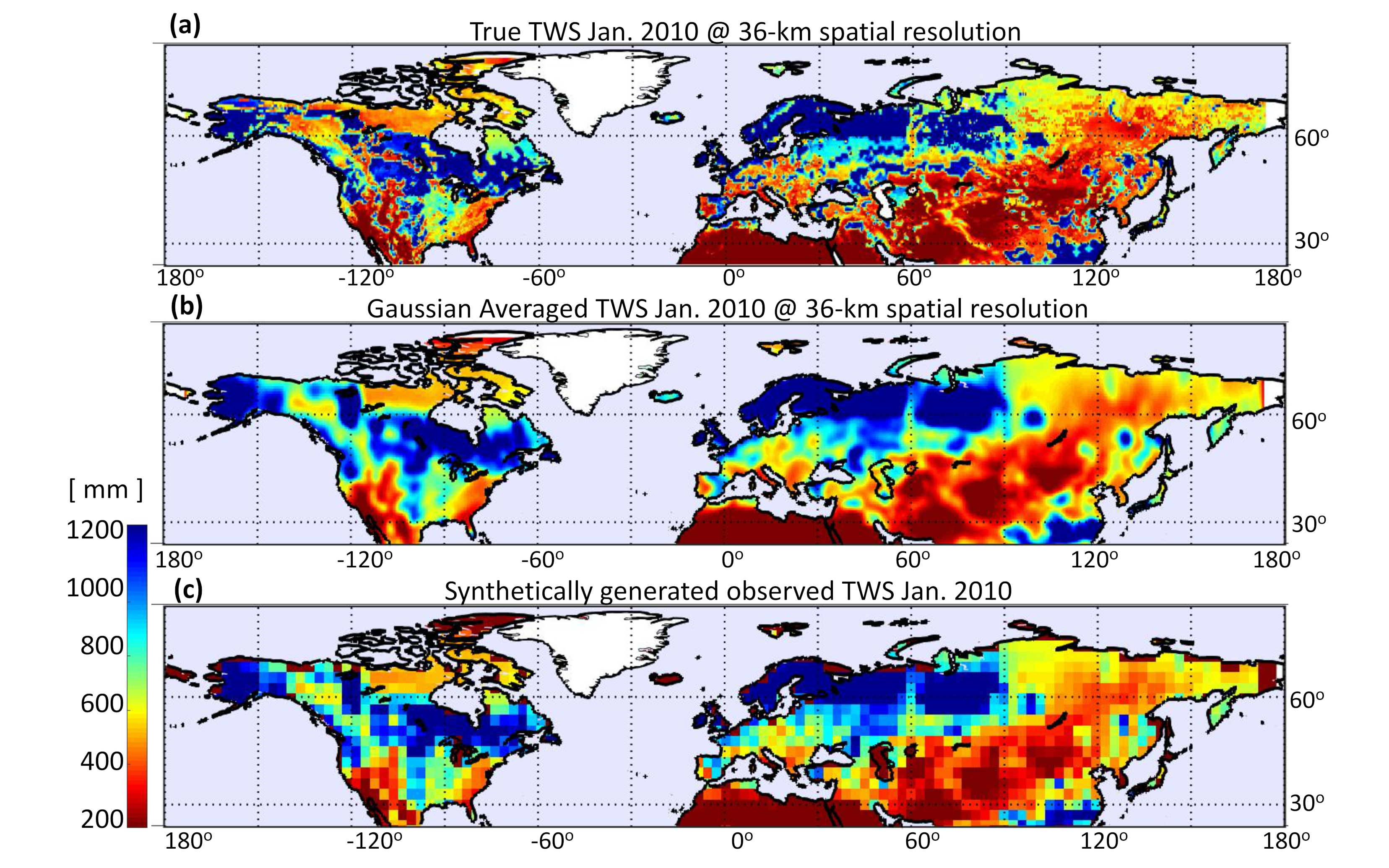
The suite of synthetic diagnostic variables includes estimates of TWS at the model spatial resolutions (i.e., 36 km). From these, we generated synthetic TWS observations (Z) via temporal and spatial averages. Temporal- and spatial-averaging and re-gridding were necessary to reproduce GRACE-like synthetic observations. Temporally, we aggregated TWS values to 1-month 1-month (Figure 2a) and spatially, apply a Gaussian smoother with a 300-km half-width on the 36-km modeled TWS (Figure 2b) and finally sub-sampled the smoothed TWS values at 3 × 3 degrees spacing (Figure 2c) to approximately match the spatial resolution of GRACE operational products (e.g., [2,3,48,49]). Note, that GRACE-derived TWS retrievals are usually expressed in terms of anomalies with respect to a specific reference time. Prior to data assimilation, we converted the TWS anomalies into absolute TWS values based on a model estimate of TWS at the reference time. This common practice is equivalent to confronting the anomalies of the model estimates with the original anomaly TWS retrievals in that only TWS anomaly information is assimilated. In the proposed synthetic assimilation approach (Section 3.3), sources of errors were known and only attributed to precipitation fluxes, thus we arbitrarily used a measurement error equal to 5 mm.

3.2. Ensemble Simulation

In general, any land surface model determines TWS from the mass balance equation:
d T W S ( t ) d t = [ P ( t ) E ( t ) R ( t ) ] d t
This means that for a specific model time step t the uncertainties associated with the estimation of TWS depended upon errors/uncertainties in the precipitation (P), evaporation (E), and runoff (R) fluxes on the right-hand side of Equation (1). In this study, we focused on the error dependencies between TWS and precipitation fluxes and assume dthat the only source of modeling errors was inaccurate precipitation input. While precipitation errors were likely to dominate in GRACE data assimilation, this assumption was nevertheless a simplification that was not fully representative of reality. The assumption was, however, useful for testing the feasibility of the proposed assimilation method in our synthetic experiment. In our ensemble-based data assimilation system, the precipitation errors could be represented through the generation of an ensemble of equiprobable model realizations. We generated an ensemble of 24 members ([5]) of possible precipitation realizations using a multiplicative error scheme as follows:
P j , m = b j , m · P M 2 , m
where the subscript j = 1 , 2 , , 24 indicates the ensemble member, P M 2 , m is the nominal precipitation forcing (in this case, MERRA-2 precipitation, Section 2), and b j , m is the precipitation error coefficient for a given ensemble member j and month m. These error coefficients were sampled at the beginning of each month m from a lognormal distribution with mean = 1.0 and coefficient of variation = 0.5, which implies that the perturbations corresponded to 50% of the magnitude of the nominal MERRA-2 precipitation. This approach has been extensively used in previous efforts to generate an ensemble of precipitation forcings (e.g., [4,50,51,52,53]). Horizontal correlation of the precipitation errors ( b j , m ) is isotropic with a 2-degree correlation length ([5]). We assumed that errors in the precipitation forcing were perfectly correlated within 1 month. This assumption helped to assess the feasibility of using GRACE for improving precipitation estimates by narrowing its uncertainties and allowed systematic updating of the precipitation errors ( b j , m ) using the monthly GRACE-like synthetic observations.
With these settings we generated an ensemble of model realizations, hereafter referred to as the open-loop (or model only) simulation, which included monthly estimates of TWS, along with soil moisture at different soil levels (surface, rootzone), and all associated fluxes (e.g., precipitation, runoff, evaporation) for July 2003–July 2016.

3.3. Data Assimilation Approach

The proposed data assimilation approach was broadly similar to existing GRACE data assimilation schemes (e.g., [4,5,9,41]), except that we update errors in precipitation fluxes instead of the TWS prognostic states (i.e., soil moisture and snow). That is, we employed a two-step, ensemble smoothing approach in which the land model integration was performed twice over the course of the same month: first to collect monthly TWS observations minus predicted differences, and a second time to update that month’s simulated TWS. Details of the assimilation methodology can be found in [5]. As in [5], CLSM computed, for each model grid cell and every 7.5 min, an ensemble of TWS estimates that were driven by the ensemble of precipitation forcings (Equations (1) and (2)). At the end of each month, these estimates were aggregated in space and time to compute monthly TWS observation predictions ( M ( b j , m ) )), which were the model’s best guess of the synthetic observations. Both the spatial- and the temporal-averaging procedures were the same as those used for the generation of the synthetic observations (Z, Section 3.1.1). The ensemble-based analysis used these observation predictions to compute precipitation error increments:
b j , m + b j , m = K [ Z j M ( b j , m ) ]
where the superscripts “+” and “−” in the monthly precipitation error coefficients ( b j , m ) refer to the assimilation (or posterior) and open-loop (or prior assimilation) ensembles, respectively. In Equation (3), GRACE-like synthetic TWS observations ( Z j ) were also perturbed according to [54] using the measurement error (Section 3.1.1). The array K represents the Kalman gain, which controlled the magnitude of the precipitation error increments ( b j , m + b j , m ), and was calculated as:
K = C b M [ R + C M M ] 1
where R is the measurement error covariance (a diagonal matrix with non-zero elements equal to the measurement error), and C M M is the sample error covariance of the observation predictions. C M M is simply obtained as a covariance matrix from the observation predictions M ( b j , m ) . Thus, the key technical difference with respect to previously developed GRACE data assimilation efforts was in the calculation of the cross-covariance matrix C b M , the error covariance term computed between the forecast observation predictions ( M ( b j , m ) ) and the precipitation error coefficients ( b j , m ). This was different from previous studies which instead computed this cross-covariance directly from the ensemble of the TWS prognostic variable states (e.g., groundwater, soil moisture, snow, etc.) and the observation predictions while updating the prognostic states directly.
After computing the precipitation error increments (Equation (3)), we rewound the model to the beginning of the month and re-ran the same month with the updated precipitation errors. Under the assumption that TWS errors retained information of the precipitation errors, the rewound run should include a more realistic precipitation input, as the assimilation step minimized the differences between modeled and observed (synthetic) TWS. The data assimilation run produced a series of estimates of precipitation errors, along with fluxes (precipitation, evaporation, runoff), and prognostic variables (snow, soil moisture) over the same period as the open-loop, from July 2003 to July 2016. Thus, the adjusted precipitation was included among the outputs of the assimilation step.

3.4. Metrics for Performance Evaluation

We assessed the performance of the proposed assimilation scheme using the Pearson correlation coefficient (R) and the unbiased root mean-square error ( u b R M S E ,[55]), computed for both the open-loop and data assimilation experiments with respect to the set of synthetic hydrologic variables (Section 3.1). These two metrics are commonly used to evaluate modeled vs. observed hydrological estimates in terms of their dynamic variability (R) and random error ( u b R M S E ). Bias metrics were not computed as they were close to zero by the design of the synthetic experiment, and R M S E metrics were effectively equivalent to u b R M S E metrics here.

4. Results and Discussion

4.1. Verification of the Method

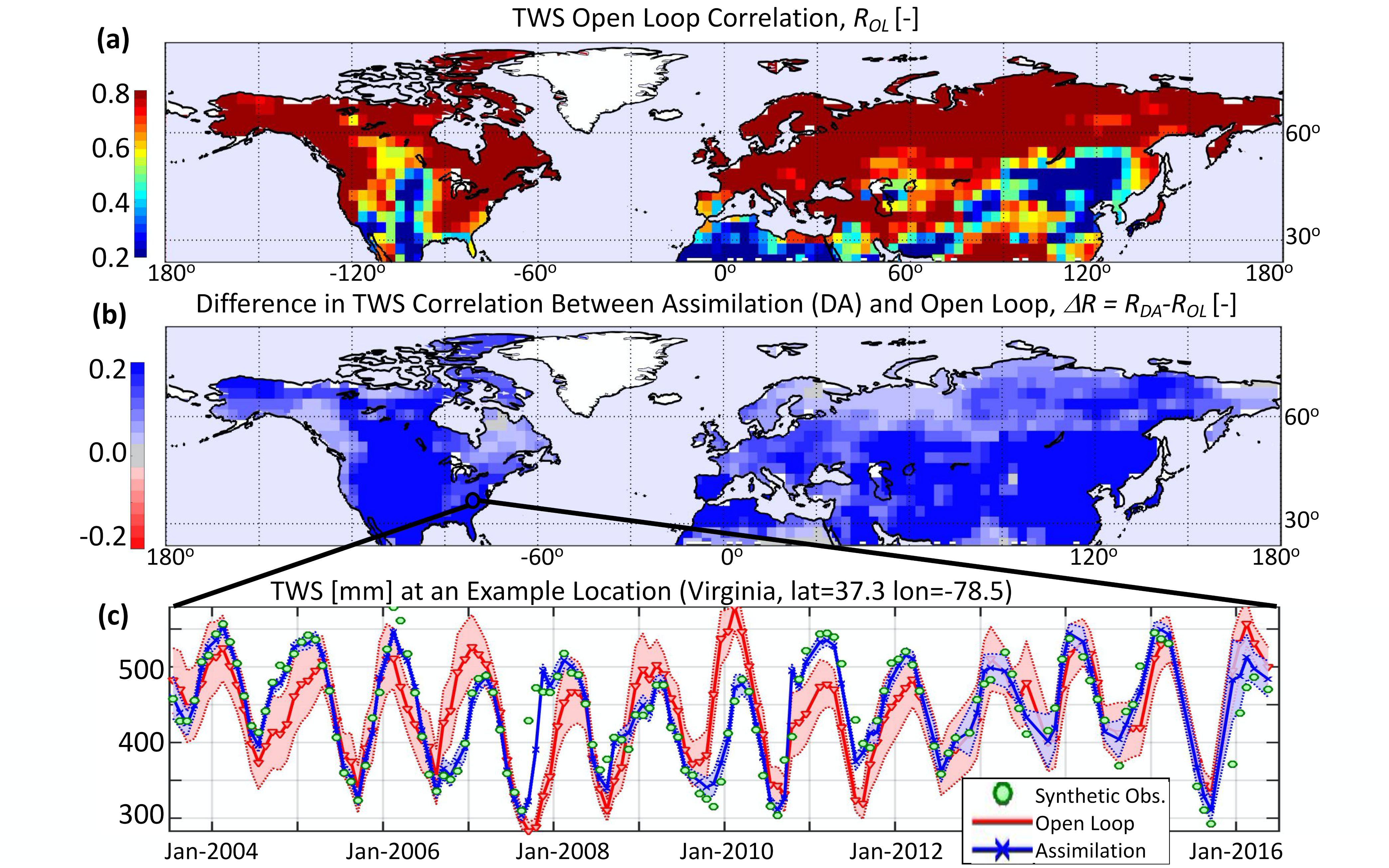
To verify that the new assimilation scheme behaves as designed, we first investigated the R and u b R M S E performance skill metrics for TWS at the spatial and temporal scales of the assimilated synthetic TWS observations. The domain average values for the R and u b R M S E are 0.70 and 39.2 mm, respectively, for the open-loop run and 0.90 and 17.5 mm for the assimilation case, which confirmed the expected overall improvement in TWS estimates from the assimilation of the synthetic TWS observations.
Figure 3a maps R values of the open-loop TWS estimates versus the synthetic truth and Figure 3b depicts the improvement of the assimilation estimates over the open loop for the R skill ( u b R M S E is not shown). Some of the low values were attributed to regions with very low precipitation (e.g., Sahara Desert, Gobi Desert), where small changes in precipitation could cause large changes in the correlation coefficients. Other differences could be attributed to the nonlinearity of the model in partitioning the precipitation input into the various TWS components. For example, the lower R values reported in the central US corresponded to regions where the depth-to-bedrock parameter was large, affecting the TWS response to changes in precipitation.
When the synthetic observations of TWS were assimilated, the R skill increased everywhere over the domain region, with some areas receiving larger increases than others. The largest improvements (darker blues in Figure 3b) correspond to regions where the open-loop TWS performs poorly (blue areas in Figure 3a). These improvements were expected because the assimilated TWS should, by design, agree better with the observed (synthetic) TWS (Figure 3c). For the sample location shown in Figure 3c, the R and u b R M S E values for the open-loop experiment were 0.61 and 58 mm. These improved in the assimilation case to 0.94 and 23 mm, respectively. In this specific example, improvements were evident in the second half of 2007, between 2009 and 2010, and again in 2011, when the assimilation of TWS matched the synthetic TWS more closely than TWS from the open-loop.
The spatial averaging process to generate GRACE-like synthetic observations (Section 3.1.1) removed the fine scale features that are present in the modeled TWS (Figure 2a). Our synthetic experiment configuration allowed us to test whether fine spatial scales could be resolved through the assimilation of coarse spatial resolution TWS into a model running at finer resolution. To test this, for each month we calculated spatial correlations between the synthetic TWS and the assimilation and open-loop TWS at the model horizontal resolution, after removing a 300 km Gaussian average from the estimates, as an attempt to isolate improvements at the finer (model) scale. The assimilation spatial correlation was always larger than the open-loop. For both experiments, values were very high with long-term average equal to 0.97 and 0.99 for open-loop and assimilation experiments, respectively. These high values were likely a consequence of the perfect knowledge of both open-loop and assimilation experiments of the synthetic model physics at the 36-km scale.

4.2. Assessment of Precipitation Errors

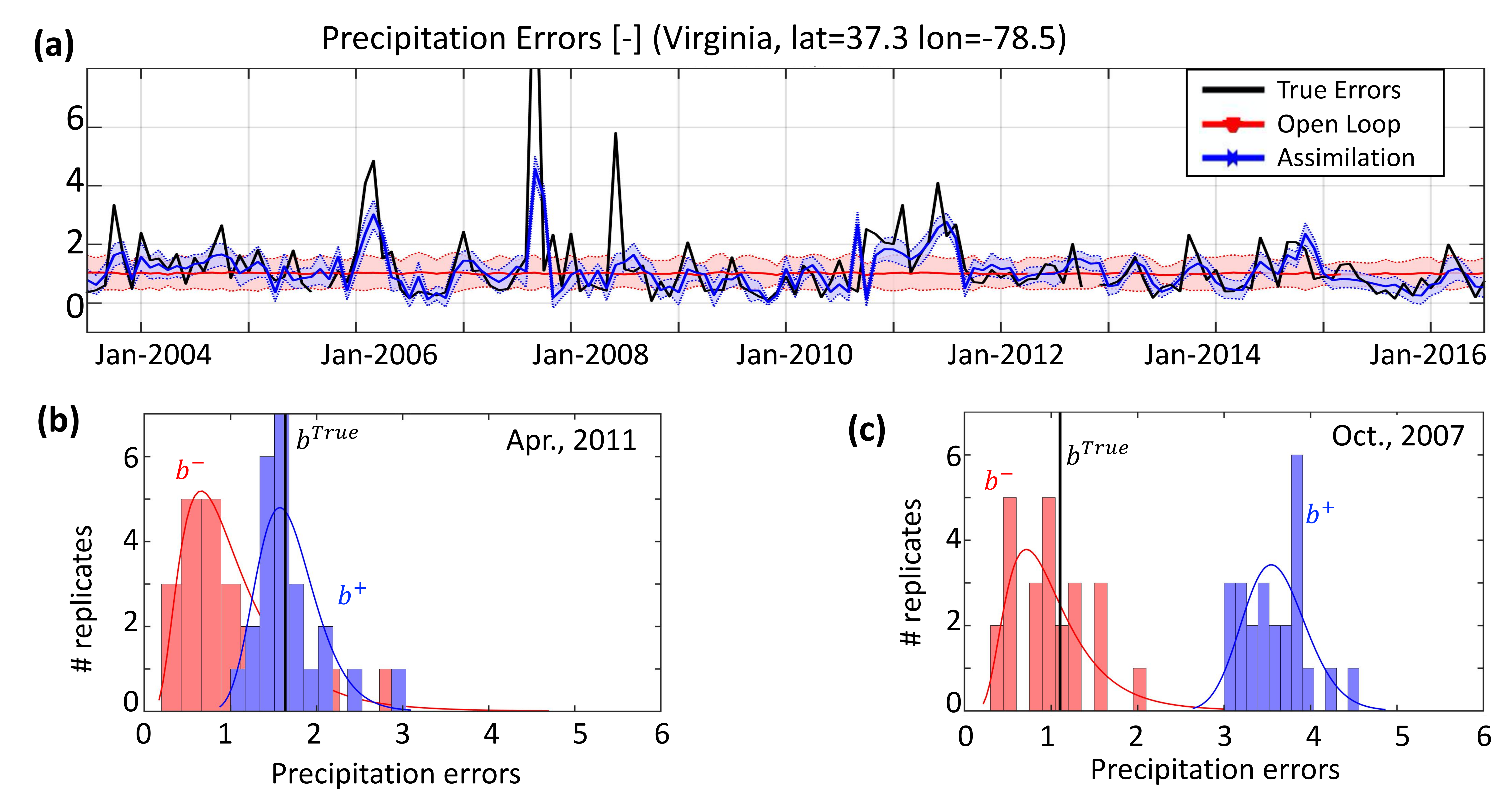
The open-loop (Section 3.2) precipitation errors were updated by the assimilation scheme (Section 3.3). The mechanism behind the precipitation error updates is illustrated for a sample location in Figure 4. The black solid lines in the figure report true-error values, determined as:
b T r u e , m = P T r u e , m P M 2 , m
where P M 2 , m is the MERRA-2 precipitation for a given month m and the synthetic “true” precipitation P T r u e , m was obtained from the 8-year shifted MERRA-2 precipitation (Section 3.1). The above ratio inevitably created some instabilities for those times when the nominal MERRA-2 precipitation ( P M 2 , m ) approached zero. To limit these instabilities, b T r u e , m we calculated and showed only for the months when P M 2 , m was greater than its temporal 1-percentile calculated for each individual model grid. For this reason, some months (i.e., September 2005 and November 2012) had missing values for b T r u e , m in Figure 4a.
By construction, the open-loop error distribution is sampled from the same lognormal distribution (Section 3.2) for each month. Thus, the open-loop sample distribution varied only minimally (because of sampling noise); its mean remained close to one (red solid line in Figure 4a) and did not follow the true precipitation errors.
For the assimilation case, the precipitation error distributions from the ensemble-based analysis (Section 3.3) followed the true errors much more closely. Nonetheless, the assimilation results could not quite retrieve some of the high values (extremes) reported in the synthetic precipitation error time-series as could be seen, for example, in September 2007 and in June 2008. In general, high values of b T r u e , m corresponded to times when synthetic precipitation (i.e., the 8-year shifted MERRA-2 precipitation) was much higher than the nominal one from MERRA-2. The ensemble-based analysis performed best under a Gaussian linear assumption which may not be met for some of these instances given the non-linearity of the land surface model. Finally, note that the ensemble spread of the assimilation was much smaller than that of the open-loop. In fact, as it combined multiple sources of information, the assimilation allowed for increased robustness (i.e., reduced uncertainty) of the estimates around the mean value.
Finally, Figure 4b,c illustrates precipitation error ensembles (or realization) of the open-loop (red) and assimilation (blue) distributions for two different months. In April 2011 (Figure 4b), the assimilation performed as planned and retrieved the synthetic precipitation error. In October 2007 (Figure 4c), however, the assimilation failed to retrieve the true errors and the open-loop ensemble provided a better precipitation error’s estimate. This might have been caused by the differences in the temporal response of TWS to changes in precipitation errors. In fact, the value of b T r u e was very large for the month of September 2007 and considerably underestimated by the assimilation (and even more so by the open-loop), whereas in October 2007 the true precipitation error was very small (close to one). It is possible that the assimilation of TWS could not capture these quick changes experienced by the precipitation error.

4.3. Assessment of Storages and Fluxes

Figure 5 and Table 1 summarize the domain-average performance skill in terms of R and u b R M S E for all storage and flux variables of the water budget for the open-loop and assimilation cases. The assimilation results (blue bars in Figure 5) indicated consistently improved statistics relative to the open-loop results (red bars) for both the R and u b R M S E metrics because of the precipitation correction in the TWS assimilation scheme. These bulk statistics demonstrated that GRACE-like TWS assimilation could help correct (adjust) the precipitation forcing, which in turn enhanced TWS, snow mass, soil moisture, runoff, and evaporation estimates. Next, we investigated the spatial pattern dynamics related to fluxes and terrestrial water storage components.

4.3.1. Precipitation

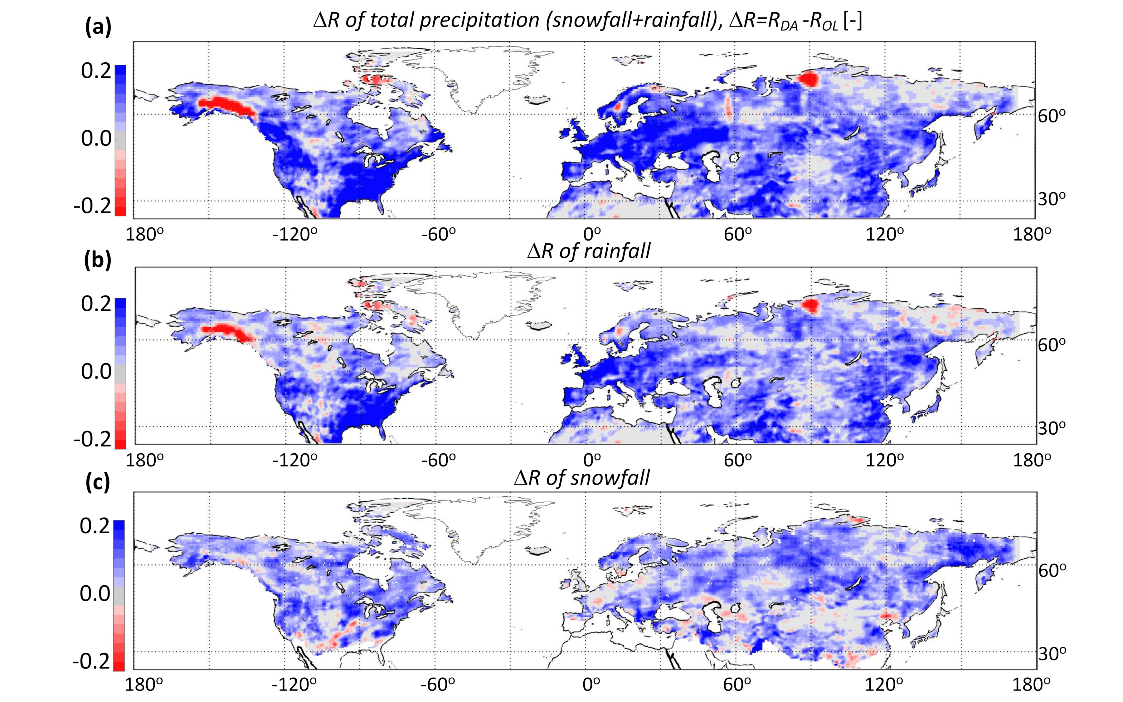
The synthetic data assimilation experiment allowed us to understand if TWS observations (in this case, synthetically derived, but similar to GRACE observations) had the capability to inform precipitation fluxes, especially in regions where precipitation observations were scarce or otherwise uncertain. Figure 6 illustrated the difference in correlation skill (vs. the synthetic observations) between the data assimilation and open-loop estimates of total precipitation (i.e., rainfall plus snowfall), snowfall only, and rainfall only. Domain-mean differences were 0.08, 0.07, 0.05 for the total precipitation, rainfall, and snowfall respectively (Table 1). Domain-mean differences in u b R M S E were −0.13 mm/d, −0.11 mm/d, and −0.03 mm/d for the total precipitation, rainfall, and snowfall respectively (Table 1). Although small, these differences (increased R and decreased u b R M S E ) confirmed an improvement thanks to data assimilation.
In general, the data assimilation scheme improved total precipitation correlations everywhere in the domain, except for a few localized regions where the skill was considerably degraded (red areas in Figure 6a). Specifically, there were large discrepancies between assimilated precipitation and the synthetic observations in some areas like around the Gulf of Alaska and in the Yenisei River Delta (Russia), mainly during the summer months. Because of this, the spatial pattern of rainfall correlation differences (Figure 6b) largely resembled that of total precipitation (Figure 6a). The Gulf of Alaska received abundant precipitation along the maritime coastal mountain range, but several kilometers inland it decreased dramatically. It is unlikely that this strong gradient in precipitation was resolved by the assimilation of coarse scale TWS observations.
The assimilation yielded improvements nearly everywhere when we looked at snowfall correlation differences (Figure 6c). This might be related to the fact that, when snowfall occurred, nearly all of the snowfall resulted in a change in TWS due to the accumulation of SWE and the fact that runoff and evaporation were typically small when the temperature was below freezing. When it rained, a substantial fraction of the rainfall evaporated and/or is converted into runoff, thus the resulting change in TWS was generally smaller than the rainfall total. The correlation differences demonstrated that, in general, TWS synthetic observations could be used to constrain precipitation if the latter was unknown or uncertain.

4.3.2. Evaporation and Runoff

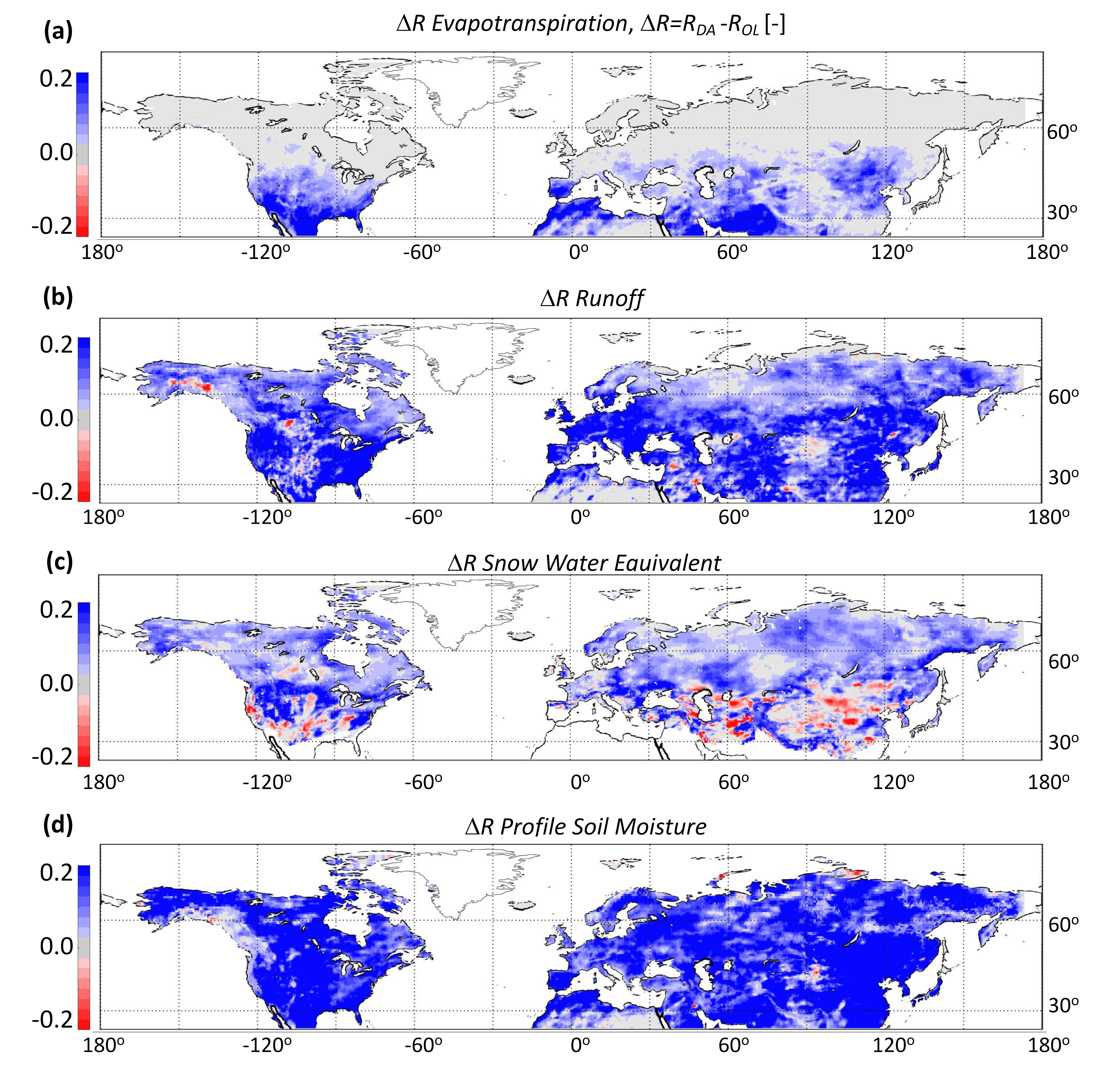
The differences in correlation between the open-loop and the assimilation results ( Δ R) for runoff and evaporation are reported in Figure 7a,b. For evaporation, the open-loop domain-average R skill equaled 0.82 and it was 0.86 for the assimilation runs. For u b R M S E , these were 0.28 mm/d for the open-loop and 0.22 mm/d for the assimilation. Only regions below about 50 N latitude showed an appreciable change in evaporation skill owing to the assimilation scheme. Evaporation changes were negligible in the high latitudes, where temperatures were substantially lower and thus, the evaporation fluxes were a minor component of the total water balance.
For runoff, the domain-average R skill equaled 0.51 for the open-loop and 0.62 for the assimilation. The corresponding u b R M S E was 0.77 mm/day for the open-loop and 0.62 mm/day for the assimilation. Runoff fluxes were improved everywhere in the study domain. By and large, the spatial patterns in these maps corresponded to those seen in the difference map for the precipitation fluxes (Figure 6). Not surprisingly, improved precipitation fluxes corresponded to better runoff estimates, which would only have been marginally possible with the traditional GRACE data assimilation approaches. In the latter, runoff changes would have been limited to improvements in baseflow and would not capture surface runoff, which, for the most part, dominates the total runoff signal. Regions of degradation include a few sporadic areas where the runoff Δ R is negative (red area in Figure 7b), such as the coast of the Gulf of Alaska, where precipitation (rainfall) fluxes experienced degradation as well (Section 4.3.1).

4.3.3. TWS Storage Components

Here, we focused on analyzing the TWS components in terms of snow water equivalent (SWE) and p r m c . The p r m c could be used as a proxy for both groundwater table and unsaturated zone soil moisture dynamics (Section 2).
The SWE domain-average R skill equaled 0.67 for the open-loop and 0.72 for the assimilation. The u b R M S E was 22.8 mm for the open-loop and 16.1 mm for the assimilation. Correlation metrics of simulated SWE with the synthetic observations improved over most of the domain, except for some low latitude areas where the SWE was not likely one of the main components of TWS. These patterns of SWE improvement (Figure 7c) often resemble those for snowfall (Figure 6c).
In general, TWS skill improvement (Figure 3b) resembles that obtained in the p r m c (Figure 7d). For the p r m c , the open-loop domain-average R skill equaled 0.54 and it was 0.73 for the assimilation runs. For u b R M S E , these were 0.020 m 3 m 3 for the open-loop and 0.014 m 3 m 3 for the assimilation. The assimilation yielded improvements nearly everywhere in the study domain, and the patterns of these changes were very similar to those seen in TWS. This is not surprising, given that the p r m c encompasseed shallow groundwater and unsaturated soil moisture.

5. Summary and Conclusions

The GRACE and GRACE-FO satellite missions have been measuring TWS globally for nearly two decades at spatial and temporal resolutions that are often considered too coarse for practical hydrological applications. State-of-the-art data assimilation methods have proven effective for spatial and temporal downscaling through direct updates to the TWS prognostic variables (i.e., soil moisture, groundwater, snow states, and surface water). This work presents an alternative approach in which the TWS data assimilation scheme adjusts errors in precipitation fluxes instead of the land model prognostic variables that make up TWS. The proposed method has the main advantage of adjusting water fluxes and states according to physically-based principles encoded in the land model as opposed to the statistically-based water increments obtained in the traditional GRACE assimilation schemes. In this way, this alternative assimilation method ensures the closure of the model internal water budget. Additionally, model fluxes such as runoff and evaporation are automatically and directly modified in response to the adjusted precipitation inputs and according to model physics.
To assess the potential of the proposed approach, we conducted a synthetic experiment where the ensemble of precipitation errors is sampled from a lognormal distribution. Under the assumption that TWS errors retain information of the precipitation errors, the assimilation scheme updates these errors using an ensemble-based analysis approach. Our main findings can be summarized as follows:
  • On average, the assimilation can retrieve reasonable precipitation errors. However, when the true errors are high, the assimilation does not always recover high enough error estimates. This might be during times when the nominal MERRA-2 precipitation is very low and the synthetic precipitation error is high.
  • The improvements in precipitation estimates are more robust for snowfall than for rainfall. Degradations sometimes occur over regions where there is a strong horizontal gradient in precipitation. Nonetheless, our results suggest that the proposed TWS assimilation technique can improve precipitation flux estimates. This is consistent with earlier studies ([37,38]) that concluded that GRACE observations could be beneficial in constraining precipitation fluxes in regions with large uncertainties (e.g., due to a scarcity of in situ data).
  • The assimilation procedure improves estimates of evaporation, runoff, SWE and profile soil moisture, thus demonstrating the feasibility of the proposed approach as an alternative to directly updating the TWS states in land surface models. This mechanism may work best where the precipitation fluxes are the main driver of errors in the water budget.
In conclusion, the results presented here demonstrate that the assimilation of synthetic TWS observations can correct (adjust) the model’s precipitation forcing and in turn enhance model estimates of TWS, soil moisture, snow mass, runoff, and evaporation. Because of this, the proposed approach has a more positive impact on simulated runoff than the standard GRACE data assimilation techniques in which TWS is updated directly. Our findings further demonstrate the benefits of GRACE assimilation on land surface model simulations, thus adding to the myriad ways that GRACE TWS retrievals have been harnessed to improve our knowledge of the terrestrial hydrologic cycle. Nonetheless, this work only presents a synthetic experiment and future work will have to test these findings using real data. Finally, an inherent assumption of the proposed synthetic data assimilation scheme is that all model errors arise from errors in the precipitation forcing, which are the largest source of error. Future work will need to address other unaccounted sources of errors (e.g., in the model inputs and parameters) for estimating TWS and related water storages and fluxes.

Author Contributions

Conceptualization, M.G. and M.R.; original draft preparation, M.G.; M.G., R.R., M.R. and V.M. have contributed to review and editing; All authors have read and agreed to the published version of the manuscript.

Funding

This study was supported by the NASA Terrestrial Hydrology and GRACE and GRACE Follow-On Science Team programs.

Acknowledgments

Computational resources were provided by the NASA High-End Computing Program through the NASA Center for Climate Simulation at the Goddard Space Flight Center.

Conflicts of Interest

The authors declare no conflict of interest.

References

  1. Tapley, B.D.; Bettadpur, S.; Ries, J.C.; Thompson, P.F.; Watkins, M.M. GRACE measurements of mass variability in the Earth system. Science 2004, 305, 503–505. [Google Scholar] [CrossRef] [Green Version]
  2. Landerer, F.W.; Flechtner, F.M.; Save, H.; Webb, F.H.; Bandikova, T.; Bertiger, W.I.; Bettadpur, S.V.; Byun, S.H.; Dahle, C.; Dobslaw, H.; et al. Extending the global mass change data record: GRACE Follow-On instrument and science data performance. Geophys. Res. Lett. 2020, 47, e2020GL088306. [Google Scholar] [CrossRef]
  3. Save, H.; Bettadpur, S.; Tapley, B.D. High-resolution CSR GRACE RL05 mascons. J. Geophys. Res. Solid Earth 2016, 121, 7547–7569. [Google Scholar] [CrossRef]
  4. Zaitchik, B.F.; Rodell, M.; Reichle, R.H. Assimilation of GRACE terrestrial water storage data into a land surface model: Results for the Mississippi River basin. J. Hydrometeorol. 2008, 9, 535–548. [Google Scholar] [CrossRef]
  5. Girotto, M.; De Lannoy, G.J.; Reichle, R.H.; Rodell, M. Assimilation of gridded terrestrial water storage observations from GRACE into a land surface model. Water Resour. Res. 2016, 52, 4164–4183. [Google Scholar] [CrossRef] [Green Version]
  6. Kumar, S.V.; Zaitchik, B.F.; Peters-Lidard, C.D.; Rodell, M.; Reichle, R.; Li, B.; Jasinski, M.; Mocko, D.; Getirana, A.; De Lannoy, G.; et al. Assimilation of gridded GRACE terrestrial water storage estimates in the North American Land Data Assimilation System. J. Hydrometeorol. 2016, 17, 1951–1972. [Google Scholar] [CrossRef]
  7. Reichle, R.H. Data assimilation methods in the Earth sciences. Adv. Water Resour. 2008, 31, 1411–1418. [Google Scholar] [CrossRef]
  8. Nair, A.S.; Indu, J. Improvement of land surface model simulations over India via data assimilation of satellite-based soil moisture products. J. Hydrol. 2019, 573, 406–421. [Google Scholar] [CrossRef]
  9. Houborg, R.; Rodell, M.; Li, B.; Reichle, R.; Zaitchik, B.F. Drought indicators based on model-assimilated Gravity Recovery and Climate Experiment (GRACE) terrestrial water storage observations. Water Resour. Res. 2012, 48. [Google Scholar] [CrossRef] [Green Version]
  10. Li, B.; Rodell, M.; Zaitchik, B.F.; Reichle, R.H.; Koster, R.D.; van Dam, T.M. Assimilation of GRACE terrestrial water storage into a land surface model: Evaluation and potential value for drought monitoring in western and central Europe. J. Hydrol. 2012, 446, 103–115. [Google Scholar] [CrossRef] [Green Version]
  11. Schumacher, M.; Forootan, E.; van Dijk, A.I.; Schmied, H.M.; Crosbie, R.S.; Kusche, J.; Döll, P. Improving drought simulations within the Murray-Darling Basin by combined calibration/assimilation of GRACE data into the WaterGAP Global Hydrology Model. Remote Sens. Environ. 2018, 204, 212–228. [Google Scholar] [CrossRef] [Green Version]
  12. Forootan, E.; Khaki, M.; Schumacher, M.; Wulfmeyer, V.; Mehrnegar, N.; van Dijk, A.I.; Brocca, L.; Farzaneh, S.; Akinluyi, F.; Ramillien, G.; et al. Understanding the global hydrological droughts of 2003–2016 and their relationships with teleconnections. Sci. Total Environ. 2019, 650, 2587–2604. [Google Scholar] [CrossRef] [Green Version]
  13. Getirana, A.; Rodell, M.; Kumar, S.; Beaudoing, H.K.; Arsenault, K.; Zaitchik, B.; Save, H.; Bettadpur, S. GRACE Improves Seasonal Groundwater Forecast Initialization over the United States. J. Hydrometeorol. 2020, 21, 59–71. [Google Scholar] [CrossRef]
  14. Rodell, M.; Famiglietti, J.S.; Wiese, D.N.; Reager, J.; Beaudoing, H.K.; Landerer, F.W.; Lo, M.H. Emerging trends in global freshwater availability. Nature 2018, 557, 651–659. [Google Scholar] [CrossRef]
  15. Khaki, M.; Forootan, E.; Kuhn, M.; Awange, J.; van Dijk, A.I.; Schumacher, M.; Sharifi, M.A. Determining water storage depletion within Iran by assimilating GRACE data into the W3RA hydrological model. Adv. Water Resour. 2018, 114, 1–18. [Google Scholar] [CrossRef] [Green Version]
  16. Reager, J.; Thomas, B.; Famiglietti, J. River basin flood potential inferred using GRACE gravity observations at several months lead time. Nat. Geosci. 2014, 7, 588–592. [Google Scholar] [CrossRef]
  17. Tangdamrongsub, N.; Steele-Dunne, S.C.; Gunter, B.C.; Ditmar, P.G.; Sutanudjaja, E.H.; Sun, Y.; Xia, T.; Wang, Z. Improving estimates of water resources in a semi-arid region by assimilating GRACE data into the PCR-GLOBWB hydrological model. Hydrol. Earth Syst. Sci. 2017, 21, 2053–2074. [Google Scholar] [CrossRef] [Green Version]
  18. Khaki, M.; Awange, J. Improved remotely sensed satellite products for studying Lake Victoria’s water storage changes. Sci. Total Environ. 2019, 652, 915–926. [Google Scholar] [CrossRef] [PubMed]
  19. Felfelani, F.; Wada, Y.; Longuevergne, L.; Pokhrel, Y.N. Natural and human-induced terrestrial water storage change: A global analysis using hydrological models and GRACE. J. Hydrol. 2017, 553, 105–118. [Google Scholar] [CrossRef] [Green Version]
  20. Girotto, M.; De Lannoy, G.J.; Reichle, R.H.; Rodell, M.; Draper, C.; Bhanja, S.N.; Mukherjee, A. Benefits and pitfalls of GRACE data assimilation: A case study of terrestrial water storage depletion in India. Geophys. Res. Lett. 2017, 44, 4107–4115. [Google Scholar] [CrossRef] [PubMed] [Green Version]
  21. Van Dijk, A.; Renzullo, L.; Wada, Y.; Tregoning, P. A global water cycle reanalysis (2003–2012) merging satellite gravimetry and altimetry observations with a hydrological multi-model ensemble. Hydrol. Earth Syst. Sci. 2014, 18, 2955–2973. [Google Scholar] [CrossRef] [Green Version]
  22. Rodell, M.; Beaudoing, H.K.; L’Ecuyer, T.; Olson, W.S.; Famiglietti, J.S.; Houser, P.R.; Adler, R.; Bosilovich, M.G.; Clayson, C.A.; Chambers, D.; et al. The observed state of the water cycle in the early twenty-first century. J. Clim. 2015, 28, 8289–8318. [Google Scholar] [CrossRef]
  23. Khaki, M.; Hoteit, I.; Kuhn, M.; Awange, J.; Forootan, E.; Van Dijk, A.I.; Schumacher, M.; Pattiaratchi, C. Assessing sequential data assimilation techniques for integrating GRACE data into a hydrological model. Adv. Water Resour. 2017, 107, 301–316. [Google Scholar] [CrossRef] [Green Version]
  24. Eicker, A.; Jensen, L.; Wöhnke, V.; Dobslaw, H.; Kvas, A.; Mayer-Gürr, T.; Dill, R. Daily GRACE satellite data evaluate short-term hydro-meteorological fluxes from global atmospheric reanalyses. Sci. Rep. 2020, 10, 4504. [Google Scholar] [CrossRef]
  25. Hossain, F.; Anagnostou, E.N. Numerical investigation of the impact of uncertainties in satellite rainfall estimation and land surface model parameters on simulation of soil moisture. Adv. Water Resour. 2005, 28, 1336–1350. [Google Scholar] [CrossRef]
  26. Derin, Y.; Anagnostou, E.; Berne, A.; Borga, M.; Boudevillain, B.; Buytaert, W.; Chang, C.H.; Delrieu, G.; Hong, Y.; Hsu, Y.C.; et al. Multiregional satellite precipitation products evaluation over complex terrain. J. Hydrometeorol. 2016, 17, 1817–1836. [Google Scholar] [CrossRef]
  27. Maggioni, V.; Massari, C. On the performance of satellite precipitation products in riverine flood modeling: A review. J. Hydrol. 2018, 558, 214–224. [Google Scholar] [CrossRef]
  28. Derin, Y.; Anagnostou, E.; Berne, A.; Borga, M.; Boudevillain, B.; Buytaert, W.; Chang, C.H.; Chen, H.; Delrieu, G.; Hsu, Y.C.; et al. Evaluation of GPM-era global satellite precipitation products over multiple complex terrain regions. Remote Sens. 2019, 11, 2936. [Google Scholar] [CrossRef] [Green Version]
  29. Shrestha, A.; Nair, A.S.; Indu, J. Role of precipitation forcing on the uncertainty of land surface model simulated soil moisture estimates. J. Hydrol. 2020, 580, 124264. [Google Scholar] [CrossRef]
  30. Tang, G.; Clark, M.P.; Papalexiou, S.M.; Ma, Z.; Hong, Y. Have satellite precipitation products improved over last two decades? A comprehensive comparison of GPM IMERG with nine satellite and reanalysis datasets. Remote Sens. Environ. 2020, 240, 111697. [Google Scholar] [CrossRef]
  31. Wanders, N.; Pan, M.; Wood, E.F. Correction of real-time satellite precipitation with multi-sensor satellite observations of land surface variables. Remote Sens. Environ. 2015, 160, 206–221. [Google Scholar] [CrossRef]
  32. Román-Cascón, C.; Pellarin, T.; Gibon, F.; Brocca, L.; Cosme, E.; Crow, W.; Fernández-Prieto, D.; Kerr, Y.H.; Massari, C. Correcting satellite-based precipitation products through SMOS soil moisture data assimilation in two land-surface models of different complexity: API and SURFEX. Remote Sens. Environ. 2017, 200, 295–310. [Google Scholar] [CrossRef]
  33. Crow, W.; Ryu, D. A new data assimilation approach for improving hydrologic prediction using remotely-sensed soil moisture retrievals. Hydrol. Earth Syst. Sci. 2009, 13, 1–16. [Google Scholar] [CrossRef] [Green Version]
  34. Crow, W.T.; Huffman, G.J.; Bindlish, R.; Jackson, T.J. Improving satellite-based rainfall accumulation estimates using spaceborne surface soil moisture retrievals. J. Hydrometeorol. 2009, 10, 199–212. [Google Scholar] [CrossRef] [Green Version]
  35. Becker, M.; LLovel, W.; Cazenave, A.; Güntner, A.; Crétaux, J.F. Recent hydrological behavior of the East African great lakes region inferred from GRACE, satellite altimetry and rainfall observations. Comptes Rendus Geosci. 2010, 342, 223–233. [Google Scholar] [CrossRef]
  36. Humphrey, V.; Gudmundsson, L.; Seneviratne, S.I. A global reconstruction of climate-driven subdecadal water storage variability. Geophys. Res. Lett. 2017, 44, 2300–2309. [Google Scholar] [CrossRef]
  37. Behrangi, A.; Gardner, A.; Reager, J.T.; Fisher, J.B.; Yang, D.; Huffman, G.J.; Adler, R.F. Using GRACE to estitmate snowfall accumulation and assess gauge undercatch corrections in high latitudes. J. Clim. 2018, 31, 8689–8704. [Google Scholar] [CrossRef]
  38. Robinson, E.L.; Clark, D.B. Using Gravity Recovery and Climate Experiment data to derive corrections to precipitation data sets and improve modelled snow mass at high latitudes. Hydrol. Earth Syst. Sci. 2020, 24, 1763–1779. [Google Scholar] [CrossRef] [Green Version]
  39. Swenson, S. Assessing high-latitude winter precipitation from global precipitation analyses using GRACE. J. Hydrometeorol. 2010, 11, 405–420. [Google Scholar] [CrossRef]
  40. Maggioni, V.; Anagnostou, E.; Reichle, R. The impact of model and rainfall forcing errors on characterizing soil moisture uncertainty in land surface modeling. Hydrol. Earth Syst. Sci. 2012, 16, 3499–3515. [Google Scholar] [CrossRef] [Green Version]
  41. Forman, B.A.; Reichle, R.; Rodell, M. Assimilation of terrestrial water storage from GRACE in a snow-dominated basin. Water Resour. Res. 2012, 48. [Google Scholar] [CrossRef] [Green Version]
  42. Koster, R.D.; Suarez, M.J.; Ducharne, A.; Stieglitz, M.; Kumar, P. A catchment-based approach to modeling land surface processes in a general circulation model: 1. Model structure. J. Geophys. Res. Atmos. (1984–) 2000, 105, 24809–24822. [Google Scholar] [CrossRef]
  43. Girotto, M.; Reichle, R.H.; Rodell, M.; Liu, Q.; Mahanama, S.; De Lannoy, G.J. Multi-sensor assimilation of SMOS brightness temperature and GRACE terrestrial water storage observations for soil moisture and shallow groundwater estimation. Remote Sens. Environ. 2019, 227, 12–27. [Google Scholar] [CrossRef]
  44. Brodzik, M.J.; Billingsley, B.; Haran, T.; Raup, B.; Savoie, M.H. EASE-Grid 2.0: Incremental but significant improvements for Earth-gridded data sets. ISPRS Int. J. Geo-Inf. 2012, 1, 32–45. [Google Scholar] [CrossRef] [Green Version]
  45. Reichle, R.H.; Liu, Q.; Koster, R.D.; Crow, W.T.; De Lannoy, G.J.; Kimball, J.S.; Ardizzone, J.V.; Bosch, D.; Colliander, A.; Cosh, M.; et al. Version 4 of the SMAP Level-4 Soil Moisture algorithm and data product. J. Adv. Model. Earth Syst. 2019, 11, 3106–3130. [Google Scholar] [CrossRef] [Green Version]
  46. Gelaro, R.; McCarty, W.; Suárez, M.J.; Todling, R.; Molod, A.; Takacs, L.; Randles, C.A.; Darmenov, A.; Bosilovich, M.G.; Reichle, R.; et al. The modern-era retrospective analysis for research and applications, version 2 (MERRA-2). J. Clim. 2017, 30, 5419–5454. [Google Scholar] [CrossRef]
  47. Reichle, R.H.; Liu, Q.; Koster, R.D.; Draper, C.S.; Mahanama, S.P.; Partyka, G.S. Land surface precipitation in MERRA-2. J. Clim. 2017, 30, 1643–1664. [Google Scholar] [CrossRef]
  48. Watkins, M.M.; Wiese, D.N.; Yuan, D.N.; Boening, C.; Landerer, F.W. Improved methods for observing Earth’s time variable mass distribution with GRACE using spherical cap mascons. J. Geophys. Res. Solid Earth 2015, 120, 2648–2671. [Google Scholar] [CrossRef]
  49. Loomis, B.; Luthcke, S.; Sabaka, T. Regularization and error characterization of GRACE mascons. J. Geod. 2019, 93, 1381–1398. [Google Scholar] [CrossRef]
  50. Maggioni, V.; Reichle, R.H.; Anagnostou, E.N. The effect of satellite rainfall error modeling on soil moisture prediction uncertainty. J. Hydrometeorol. 2011, 12, 413–428. [Google Scholar] [CrossRef]
  51. Girotto, M.; Margulis, S.A.; Durand, M. Probabilistic SWE reanalysis as a generalization of deterministic SWE reconstruction techniques. Hydrol. Process. 2014, 28, 3875–3895. [Google Scholar] [CrossRef]
  52. Margulis, S.A.; Girotto, M.; Cortés, G.; Durand, M. A particle batch smoother approach to snow water equivalent estimation. J. Hydrometeorol. 2015, 16, 1752–1772. [Google Scholar] [CrossRef]
  53. Reichle, R.H.; De Lannoy, G.J.; Liu, Q.; Koster, R.D.; Kimball, J.S.; Crow, W.T.; Ardizzone, J.V.; Chakraborty, P.; Collins, D.W.; Conaty, A.L.; et al. Global assessment of the SMAP level-4 surface and root-zone soil moisture product using assimilation diagnostics. J. Hydrometeorol. 2017, 18, 3217–3237. [Google Scholar] [CrossRef] [PubMed]
  54. Burgers, G.; Jan van Leeuwen, P.; Evensen, G. Analysis scheme in the ensemble Kalman filter. Mon. Weather Rev. 1998, 126, 1719–1724. [Google Scholar] [CrossRef]
  55. Entekhabi, D.; Njoku, E.G.; O’Neill, P.E.; Kellogg, K.H.; Crow, W.T.; Edelstein, W.N.; Entin, J.K.; Goodman, S.D.; Jackson, T.J.; Johnson, J.; et al. The soil moisture active passive (SMAP) mission. Proc. IEEE 2010, 98, 704–716. [Google Scholar] [CrossRef]
  56. Rodell, M.; Houser, P. Updating a land surface model with MODIS-derived snow cover. J. Hydrometeorol. 2004, 5, 1064–1075. [Google Scholar] [CrossRef]
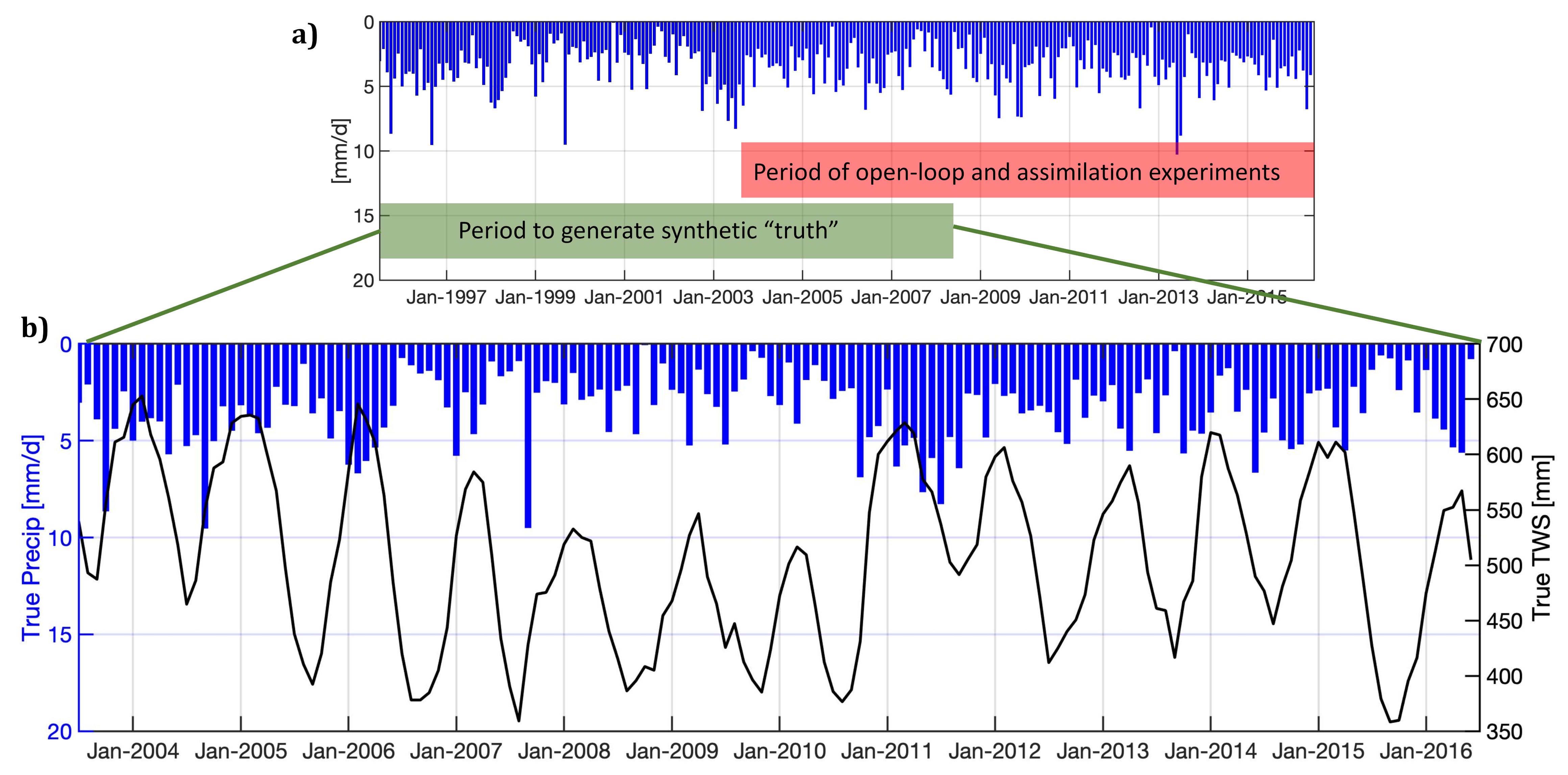
Figure 1. (a) MERRA-2 precipitation from July 1995 to July 2016. The green and red horizontal bars indicate the periods to (i) generate synthetic precipitation (July 1995–July 2008) and (ii) evaluate model and assimilation results (July 2003–July 2016), respectively. (b) Synthetically generated precipitation (blue bars) and synthetic Terrestrial Water Storage (TWS, black line) for the period of analysis (July 2003–July 2016) of a sample 36-km model grid located in Virginia, United States (37.32 N, 78.46 W).
Remotesensing 13 01223 g001
Figure 2. (a) Synthetic Terrestrial Water Storage (TWS) at the model 36-km spatial resolution for a sample month (Jan 2010); (b) As in (a) but after applying a 300-km Gaussian smoothing function; (c) Synthetically generated TWS obtained from sub-sampling (b) at 3 × 3 degree spacing. Panels (ac) illustrate the process used to generate the synthetic, GRACE-like TWS observations.
Remotesensing 13 01223 g002
Figure 3. (a) Correlation coefficient between open-loop (OL) estimates and synthetic observations of Terrestrial Water Storage (TWS). (b) Difference in correlation ( Δ R) between the data assimilation (DA) and OL TWS. Statistics are computed using 156 monthly estimates. TWS estimates from the OL and DA runs are temporally and spatially averaged and resampled to match the resolution of the synthetic observations. (c) Example TWS observations (green circles) and TWS from the open-loop (red lines) and assimilation (blue lines) experiments for a location in Virginia, United States (37.32 N, 78.46 W). Shaded areas illustrate the ensemble spread (± one ensemble standard deviation from the ensemble mean) for the open-loop (red shading) and assimilation (blue shading) experiments.
Remotesensing 13 01223 g003
Figure 4. (a) Precipitation errors ( b j , m ) at a sample location in Virginia, United States (37.32 N, 78.46 W). (b) Ensemble of the precipitation error estimates from the open-loop (red) assimilation (blue) for April 2011 and (c) October 2007. Vertical black lines in (b,c) indicates the true precipitation errors.
Remotesensing 13 01223 g004
Figure 5. Domain-average skill metrics for the assimilation (blue) and open-loop (red) experiments for TWS, snow water equivalent (SWE), snowfall (SnowF), rainfall (RainF), total precipitation (TotPPT), profile soil moisture (prmc), runoff and evaporation (Evap). Skill is measured in terms of time series (a) correlation (R) and (b) unbiased root mean square error ( u b R M S E ) vs. the synthetic true values. The assimilation skill for all variables (including precipitation fluxes) are improved compared to the open-loop.
Remotesensing 13 01223 g005
Figure 6. Difference in correlation skill ( Δ R) between data assimilation (DA) and open-loop (OL) for (a) total precipitation, (b) rainfall, and (c) snowfall, taking the synthetic precipitation as “truth”. The assimilation of TWS increases the skill over nearly the entire domain, except along the Gulf of Alaska and in the Yenisei River Delta. Only snow-possible areas as indicated in ([56]) are reported in (c).
Remotesensing 13 01223 g006
Figure 7. Difference in correlation ( Δ R) between data assimilation (DA) and open-loop (OL) for (a) Evaporation, (b) Runoff, and (c) Snow water equivalent; (d) profile soil moisture, based on the synthetic simulation. Only snow-possible areas as indicated in ([56]) are reported in (c).
Remotesensing 13 01223 g007
Table 1. Domain-average correlation coefficient (R) and unbiased root mean square error ( u b R M S E ) for open-loop (OL) and data assimilation (DA) estimates. Metrics are computed vs. the synthetic “truth” data. Confidence intervals are negligible owing to the very large sample sizes afforded by the synthetic experiment setup; statistics are computed for 156 months and averaged over 63,392 grid cells. Values for snowfall and snow water equivalent are calculated after masking impossible snow areas according to [56].
R [-] ubRMSE
OLDADA-OL OLDADA-OL
Terrestrial Water Storage at obs. scale0.700.900.20 39.2 mm17.5 mm−21.7 mm
Terrestrial Water Storage at 36 km0.590.770.17 45.5 mm29.6 mm−15.8 mm
Snow Water Equivalent0.670.720.05 22.8 mm16.1 mm−6.7 mm
Profile Soil Moisture0.540.730.19 0.020 m 3 m 3 0.014 m 3 m 3 −0.006 m 3 m 3
Tot. Precipitation0.410.500.08 1.54 mm/d1.41 mm/d−0.13 mm/d
Rainfall0.480.540.07 1.37 mm/d1.26 mm/d−0.11 mm/d
Snowfall0.380.440.05 0.63 mm/d0.60 mm/d−0.03 mm/d
Evaporation0.820.860.05 0.28 mm/d0.22 mm/d−0.06 mm/d
Runoff0.510.620.11 0.77 mm/d0.62 mm/d−0.15 mm/d
Publisher’s Note: MDPI stays neutral with regard to jurisdictional claims in published maps and institutional affiliations.