Abstract
High-spatial-resolution land-surface temperature is required for several applications such as hydrological or climate studies. Global estimates of surface temperature are available from sensors observing in the infrared (IR), but without ‘all-weather’ observing capability. Passive microwave (MW) instruments can also be used to provide surface-temperature measurements but suffer from coarser spatial resolutions. To increase their resolution, a downscaling methodology applicable over different land environments and at any time of the day is proposed. The method uses a statistical relationship between clear sky-predicting variables and clear-sky temperatures to estimate temperature patterns that can be used in conjunction with coarse measurements to create high-resolution products. Different predicting variables are tested showing the need to use IR-derived information on vegetation, temperature diurnal evolution, and a temporal information. To build a true ‘all-weather’ methodology, the effect of clouds on surface temperatures is accounted for by correcting the clear-sky diurnal cycle amplitude, using cloud parameters from meteorological reanalysis. Testing the method on a coarse IR synthetic data at ∼25 km resolution yields a Root Mean Square Deviations (RMSD) between the ∼5 km high-resolution and downscaled temperatures smaller than 1 C. When applied to observations by the Special Sensor Microwave Imager Sounder (SSMIS) at ∼25 km resolution, the downscaling to ∼5 km yields a smaller RMSD compared to IR observations. These results demonstrate the relevance of the methodology to downscale MW land-surface temperature and its potential to spatially enhanced the current ‘all-weather’ satellite monitoring of surface temperatures.
1. Introduction
Land-Surface Temperature (T) is the physical temperature of the uppermost layer of the Earth continental surfaces. It plays a key role in the land–atmosphere exchanges, driving the longwave surface-emitted radiation, and controlling the partitioning between latent and sensible heat fluxes. It is one of the Essential Climate Variable (ECV) of the Global Climate Observing System of the World Meteorological Organization [1]. Development of global, long time series of T data records is currently encouraged, but it faces difficulties. Contrarily to ocean surfaces, land surfaces have a lower heat capacity, and when exposed to solar fluxes, T undergoes strong diurnal and seasonal variations, with high spatial variability related to surface properties such as vegetation density or soil moisture [2].
T at the global scale can be estimated from satellite observations of the thermal emission in the infrared (IR) [3]. From geostationary satellites, T maps with a 15 min sampling time at ∼5 km spatial resolution are derived [4]. Higher resolutions are reached with polar orbiters (up to a few hundreds of meters), but at the expense of the revisit time [5]. However, IR cannot penetrate clouds, and consequently, T estimation from IR observations suffers from a clear-sky bias [6]. To overcome this limitation, some products use T derived from a land-surface energy balance model to fill the cloud gaps in the IR-derived T estimates (e.g., [7,8]). Alternative methods to provide ‘all-weather’ land-surface temperature rely on sensor fusion method [9,10,11], using a combination of model or IR measurements.
Satellite passive microwave (MW) observations are an attractive alternative for the T estimation under cloudy conditions, as they are much less affected by clouds than the IR. Ref. [12,13,14], or [15] developed methodologies to retrieve T from MW polar imagers such as the Special Sensor Microwave Imager (SSM/I), the Special Sensor Microwave Imager Sounder (SSMIS), or the Advanced Microwave Scanning Radiometer (AMSR). Some of these instruments have been in operation for a long time now (∼40 years), opening up the prospect of creating long term series of consistent ‘all-weather’ T estimates. However, the spatial resolution of the MW T is significantly lower than the IR one (∼25 km), and MW T is generally less accurate than the IR one due to the larger dependence on the more varying surface emissivities in the MW compared to the IR, the smaller dependence of the measurements to T, and the impact of subsurface emissions for very dry soils [16,17].
Downscaling of MW T, i.e., the increase of the spatial resolution of these products, would greatly benefit the T user community, and would facilitate the comparison of IR and MW retrievals. Downscaling has already been applied to improve the spatial resolution of the IR T itself [18,19], but in the MW it has so far been more widely applied to other parameter estimates, such as soil moisture [20,21]. Downscaling methods are typically based on establishing either a statistical relationship, or a physically based model, between the initial parameter at a coarse spatial resolution and the ancillary variables that will describe the fine spatial structures. Ref. [19,21] review different downscaling methodologies and insist on the importance of the selection of the ancillary information at high spatial resolution needed to provide the high-resolution spatial patterns. This information is typically extracted from vegetation-related satellite products derived from visible and infrared observations, or from digital elevation models. Both vegetation and elevation are expected to affect the T spatial distribution, with the vegetation increasing the surface heat capacity and the elevation decreasing the local T. Another potential source of information is the T diurnal cycle itself if it can be made available from model or observation, as the T cycle is modulated by the surface conditions [22,23].
A few attempts have already been conducted to downscale the MW T. [24] combined MW T estimates from AMSR-E observations at ∼25 km and Moderate-Resolution Imaging Spectroradiometer (MODIS) IR T at 1 km. Under cloudy sky, the high-spatial-resolution information is provided by a digital elevation map (DEM) and a linear correction is applied to correct for the altitude effect on the MW T at low spatial resolution. The retrieval is applied over China, at the overpassing times of the Aqua satellite (01:30 and 13:30). Similarly, [25] calibrated a MW T retrieval from AMSR observations with infrared MODIS and Geostationary Operational Environmental Satellite (GOES) T estimates, to fill the cloudy gaps with the MW and they used the normalized difference vegetation index (NDVI) and elevation information to downscale the MW estimates over North America. In the two methods described only static information (such as DEM or vegetation index) are used under clouds and the T patterns of cloudy scenes are expected to be the same as the ones for clear sky. An alternative is proposed by [26], also noticing that the methods adopted for downscaling MW T fail to quantify the effect of temporal variations related to the diurnal T cycle, limiting their use to a single overpassing time of the satellite. They used high-resolution vegetation, elevation information at 1 km resolution and data assimilation model outputs to downscale the MW T from AMSR-E. A decomposition of the diurnal cycle variation at each location into different components (annual variation, meteorological variation, and a daily cycle) is adopted to correct the MW-derived high-resolution T estimates and it is applied over northeastern China. However, the complex input required for this method hinder its applicability.
In this study, a simpler methodology is proposed to downscale MW T for global application, regardless of the overpassing time of the satellite, for both clear and cloudy scenes. The main benefits of this method are the possible application to different instruments, with a downscaling method valid regardless of the local time of the satellite observations. So far, only the study in [26] accounted for this issue, the other methods being specific to a given overpassing time. Within a coarse resolution MW T ground footprint, heterogeneous surfaces can have different heat capacities and related T diurnal cycles, and this must be taken into account. In addition, it is also important to develop a downscaling scheme that can operate efficiently under both clear and overcast scenes. To our knowledge, downscaling methods were so far applied to the MW T estimates, without considering the cloud cover. However, it is expected that clouds affect the local T. For instance, the study by [6], showed significantly colder daytime T under clouds than under clear conditions. This difference is expected to depend upon the surface types, with large heat capacity areas (e.g., vegetated and wet surfaces) less prone to T changes than other surfaces (such as dry arid areas), upon the cloud characteristics (e.g., its optical thickness), as well as upon the time of the day.
To obtain a high-resolution MW T product, the procedure described here relies on a statistical relationship between high-resolution ancillary information and the T estimates. This statistical function is first derived for clear-sky conditions using IR T and several ancillary products from the Spinning Enhanced Visible and Infrared Imager (SEVIRI) [27]. The original ∼5 km T estimates are used as the fine resolution T, with the coarse resolution T required to test the method being synthetically produced from aggregation of the original T to a ∼25 km resolution. For cloudy scenes, the same statistical function will be used, but with a prior correction of the input to account for the change caused by cloudy conditions. This correction is derived by studying the relationships between the downscaling inputs and cloud-relevant variables from the European Centre for Medium-Range Weather Forecasts (ECMWF) ERA5 reanalysis [28]. Finally, the downscaling with the cloud correction is illustrated by deriving a real MW T scene at ∼5 km spatial resolution from an original T scene at ∼25 km resolution from a Special Sensor Microwave Imager / Sounder (SSMIS) product currently under development by the European Space Agency (ESA) Land-Surface Temperature (LST) Climate Change Initiative (LST-CCI) project [29,30].
The study is organized as follows: the study datasets are described in Section 2, then the downscaling methods and overall processing are given in Section 3, and the methodology is evaluated in Section 4, followed by a discussion of the results obtained in Section 5. Finally, Section 6 presents the study conclusions.
2. Data
2.1. SEVIRI
Statistical downscaling relies on information at the high spatial resolution aimed for. As mentioned in the introduction, the objective is to develop a method that is flexible enough to be applicable to different local times. Therefore, satellite surface information sampled at different times of the day is required, which restricts the choice of platform to geostationary satellites. SEVIRI is selected here to provide measurements every 15 min, between N and E. The European Organization for the Exploitation of Meteorological Satellites (EUTEMSAT) Land-Surface Analysis of the Satellite Application Facility (LSA SAF) distributes SEVIRI products at ∼5 km resolution, including instantaneous T under clear-sky conditions [31]. When developing the downscaling function, these estimates will be the targeted fine spatial resolution T, while aggregation by simply averaging the ∼5 km T estimates will be used as a synthetic coarse resolution T to test the downscaling.
To characterize the surface vegetated cover, the SEVIRI 10-day average of Fraction of Vegetation Cover () representing the fraction of green vegetation per unit of horizontal soil surface [32] is selected. LSA SAF also provides several parameters that describe the median T diurnal cycle, over the same 10-day period. The SEVIRI T estimates are used to derive these parameters, assuming that the diurnal T cycle follows the model described in [23]. This simple model summarizes the diurnal cycle with a harmonic and an exponential term and is parameterized with a few parameters among which , the minimal T of the median diurnal cycle, and well as , the median amplitude of the T diurnal cycle over the same period that are considered in this study.
The SEVIRI spatial coverage does not encompass extreme latitudes but the diversity of situations is deemed enough to develop and test the methodology. Estimates of T, , , and were extracted from the LSA SAF archive for 2016. One month per season (February/May/August/November) is downloaded to capture the seasonal variability.
2.2. ERA5
To study the changes in the downscaling function inputs under cloudy conditions a dataset providing ‘all-weather’ T is required. ERA5 skin temperature, Total Column Liquid Water (), and Leaf Area Index () are available over the globe every hour at a spatial resolution of ∼25 km, and are selected here to study these changes. The resolution is lower than the one from SEVIRI, and ERA5 estimation of T does not always reproduce observed T [33]. However, the reanalysis T and cloud conditions are expected to be physically consistent and realistic enough for a first attempt to take the cloud information into account in the proposed methodology.
Similar months from 2016 are downloaded from the ECMWF archive to derive the cloud correction.
2.3. SSMIS
Once the downscaling methodology is developed using the SEVIRI and ERA5 datasets, it is applied to MW T estimates from SSMIS. The MW T estimates are based on inverting satellite observations from 19 to 90 GHz, for both perpendicular polarizations. The methodology is currently applied to the SSM/I and SSMIS time series (overpassing times around 06:00 and 18:00) as well as to AMSR data (overpassing time at 01:30 and 13:30), providing T at a spatial resolution of ∼25 km [34]. When MW T is compared with in situ T time series over a large range of environments, good agreement is typically found in vegetated environments, but larger uncertainties in the T retrievals are noted under cold conditions due to the large variability of snow and ice surface emissivities, and over very dry surfaces due to microwave penetration problems in sandy terrain [16].
To illustrate the use of the downscaling method, one day (26 November 2016) of SSMIS T retrievals for a region in Southern Africa are downloaded from the LST-CCI archive.
3. Methods and Processing
3.1. Downscaling
3.1.1. Methodology
The statistical downscaling consists of finding an estimate of T at high-resolution , given T at low-resolution and ancillary information provided at high resolution. can be written as the average of :
In Figure 1, is downscaled into 25 high-resolution pixels (N = 25), for consistency with SSMIS and SEVIRI T products at respectively ∼25 and ∼5 km.
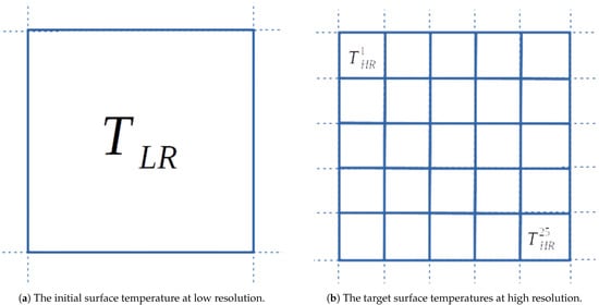
Figure 1.
Schematic of the downscaling problem.
The downscaling relies on the hypothesis that a general statistical relationship F can link the ancillary information and , to provide a high-resolution spatial pattern to be applied to low-resolution , i.e.,
For each high-resolution pixel, a correction will be applied to to describe the fine spatial structure:
It can be shown that this correction is a function of by doing:
This equation describes the increase or decrease induced by the T pattern at high resolution, computed with the average T on the pixel at low resolution as estimated by the F relationship.
3.1.2. Input Selection
The LSA SAF variables , , and at ∼5 km spatial resolution are used as the inputs to the F statistical function. Figure 2 shows the joint distribution of these variables to illustrate their relationships with T. Each variable is binned to represent the distribution of another variable under different conditions. The upper and lower quartiles (dotted lines) as well as the extrema for each distribution are shown. A positive correlation between T and is evident (upper-left panel), but similar trend is not visible between T and (upper-right). Low is associated with lower T during the day but there is no clear correlation between and T. This is expected considering that high temperatures are encountered in contrasting situations such as equatorial forest (small ) and desert regions (large ). This is corroborated by the negative correlation between and related to the lower amplitude of the diurnal cycle over vegetated areas, and the lack of correlation between T and (bottom-left). The latter shows that vegetation alone cannot be the only source of information to discriminate warm and cold temperatures, confirming the need to have more predictors than just a vegetation-related product to derive the correction.
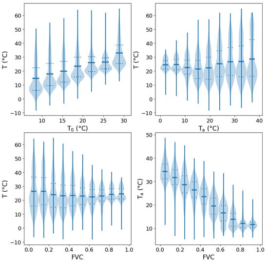
Figure 2.
High-resolution surface-temperature T as a function of the high-resolution ancillary variables suggested as predictors for the downscaling. T versus the minimal temperature () (top left), versus the amplitude of the diurnal cycle () (top right), versus the fractional vegetation cover () (bottom-left). versus is also shown (bottom-right). For each panel the distribution of the y-axis variable for a bin of value for the x-axis variable is shown in the blue shade. Additionally, the mean (solid line), upper and lower quartiles (dotted lines) are indicated, as well as the extrema of the variable.
The spatial pattern of T is expected to change with local time. For instance, rivers and arid areas can show similar T at night but very different T at midday, with the water T being rather stable during the day, but the arid area undergoing large T changes. To account for changes in the T spatial pattern with local time, a variable related to the solar radiation is added as a fourth input to the F function: the Sun elevation angle over the horizon is calculated and its sinus () is used as a continuous predictor of the spatial T pattern, to account for the local time and the season.
3.1.3. Function Implementation
The statistical function F aim is to model the relationship between the 4 inputs and T to provide the high-resolution spatial pattern to be added to the low-resolution . The function provides an absolute estimate of the temperature that is used with the low-resolution T (Equation (4)) to provide the high-resolution temperature pattern for a given pixel. Here it is implemented by a feed-forward multilayer perceptron [35], with 4 input neurons, 1 hidden layer with 10 neurons (with sigmoid activation), and 1 output. A neural network architecture can represent any continuous function given enough internal parameters [36], so it is widely used to approximate this type of mappings [19]. Its inputs are the variables , , , and , its output the , and it is trained with a database of ∼50 M data points from the 4 months in 2016 extracted from the SEVIRI archive. The SEVIRI disk is centered over the equator in Africa, and before training the original database distribution is resampled to avoid an over representation of desert situations (with very low vegetation) and a better sampling of solar elevation angles for which the low values are more common.
The residuals, i.e., the Root Mean Square Deviation (RMSD) between the targeted and the neural network output after training, are displayed for the range of T covered by the training database in Figure 3. To illustrate the choice of inputs, similar neural networks are trained using and , or only, as inputs and their residuals are displayed. Over the whole T range, the neural network using the four predictors displays a more even performance, especially for the very low and high T. It is interesting to note that on its own does not seem to be enough to provide a clear distinction between temperatures, for all hours of the day. It is also noticeable that even for the four-input neural network, the function residuals appear to be high. However, this is expected, as this function aim is not to predict the exact high-resolution T from the four ancillary variables, but rather to inform about the relative local differences related to the information content of its inputs. The result of the F model are used in the downscaling procedure (Equation (4)) and yields much lower error as apparent in Section 4.1.
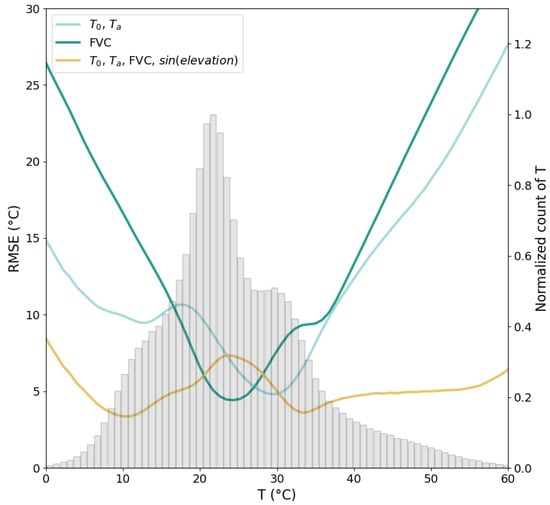
Figure 3.
Root Mean Square Deviation (RMSD) of the T estimated with the statistical function F as a function of T, for different combinations of the predicting ancillary variables. In blue F is trained with and , with only in green, and finally with , , , and in brown. The distribution of T in the testing set is shown in gray bars (labels on the right axis).
3.2. Cloud Correction
3.2.1. Methodology
Exploring T changes due to clouds for a variety of cloud and surface conditions is challenging. Isolating the cloud effect would require an estimate of T for the same area, under the same surface and insolation conditions, for different times of the day, and for a variety of cloud cover. Here the objective is only to develop a pragmatic solution that can be systematically and easily integrated into the downscaling processing. To achieve this, if the available cloud information indicates that the estimates correspond to a cloudy scene, a correction is applied to the ancillary data (that exists for clear-sky scenes) to account for the impact of the clouds on the high-resolution patterns. The correction is based on a simple function C parameterizing the cloud effect as function of the values observed for a selection of input variables , so it can be expressed as
The F statistical relationship remains unchanged, so the new correction for a cloudy scene is
3.2.2. Input Selection
ERA5 and are selected as inputs to drive the parameterization of function C. Clouds limit the amount of solar radiation on the Earth surface during daytime, with this effect depending upon the cloud optical thickness. Clouds also limit the outgoing longwave flux with a magnitude depending on cloud base height and cloud amount [37]. At the surface level, the resulting T changes will essentially depend upon the type of surface, with an expected damping of the T spatial variability compared with clear-sky conditions. This is illustrated in Figure 4, where the impact of cloudiness for two surfaces with contrasting vegetation is displayed. The distribution of , i.e., the surface T difference between clear and thin ( 50 g/m), or clear and thick ( 50 g/m) clouds are presented over evergreen forests and savanna, selected using the International Geosphere Biosphere Program (IGBP) land cover [38], at different local times. The selected times are close to the overpass time of the SSMIS and AMSR sensors and include times of day close to the minimum and maximum of the T diurnal cycle. Nighttime (01:00 and 06:00) are mostly negative, which would indicate that cloud cover tends to increase the T, due to the trapping of the thermal radiation emitted from the surface. The 06:00 negative appears to be slightly larger than the 01:00 one, which is consistent with the declining surface temperatures until the sun starts illuminating the surface again. On the other hand, daytime T seems to decrease when a cloud is present, with an effect stronger near the middle of the day (13:00), when the T diurnal cycle has its maximum. Thicker clouds can also be associated with a stronger effect, either positive or negative on . The distributions for savanna (with sparse vegetation) and evergreen forest (with a dense vegetation) are shown in Figure 4 and this also seems to have an impact on : vegetation appears to reduce the magnitude of the effect on T.
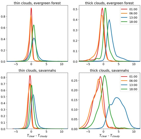
Figure 4.
Distribution of , i.e., surface-temperature difference, from ERA5 data in January, May, and September 2016. The difference is computed between clear and thin clouds ( < 50 g/m) on the first columns, and between clear and thick clouds ( > 50 g/m). The first row shows distribution over evergreen forest and the second row over savannas. Each distribution is computed at different time of the day: 01:00, 06:00, 13:00, 18:00.
Although additional effects can also affect the T distributions, Figure 4 distributions show that the variations of and vegetation can be informative enough for a first order description of the cloud impact on T. To have continuous variation on vegetation content, from ERA5 replaces the static IGBP classification.
3.2.3. Function Implementation
Figure 4 shows that the effect of clouds on nighttime is negligible compared to the one on daytime . The effect is stronger near the peak of the diurnal cycle, when the warmest T is reached. Therefore, a correction on the maximum temperature of the day driven by the and variations, which translates into a correction of the input to the F function, is proposed as an implementation for the function C.
The C function parameterization is based on the distributions shown in Figure 5. The observed difference between clear and cloudy (computed from the ERA5 dataset) for different (left panel) and (right) values is displayed. For each bin the standard deviation around the mean of the computed is shown in the solid line. As with the observations from Figure 4, the thicker the clouds and the less dense the vegetation, the larger . A polynomial parameterization derived from the distributions is also displayed as dashed lines, and it is used to practically implement the function C. The 1 uncertainty on the fitted parameters is given as a colored area around the polynomial fits. The uncertainty increases for larger and smaller , related to the smallest number of samples in the database for these extremes resulting in a more uncertain fit.

Figure 5.
Average difference of from ERA5 data from the month of January, May and September 2016 as solid lines (with 1 standard deviation) as a function of the leaf area index (LAI) (left) and total column liquid water (TCLW) (right). On each plot different colors are used for bins of TCLW (left) and LAI (right). The dotted lines show the predicted values of by the parameterization with the same input, and the shaded area shows the 1 uncertainty on the fitted parameters.
In essence, the parameterization acts as a damping coefficient reducing the amplitude of the diurnal T cycle when clouds are present. It is rather simple, but is considered efficient enough for a first order attempt to include cloud information in the downscaling scheme.
3.3. Processing
The overall processing of the downscaling scheme is illustrated in Figure 6. In a first training phase, the statistical function F is trained on a representative ensemble of LSA SAF and corresponding inputs: , , , and . Next to this, a simple correction function C is parameterized to damp the under cloudy conditions using ERA5 and . Once these functions are implemented, they can be used to downscale the in the application phase. Here, for a selected scene with a given number of estimates, the corresponding inputs , , and are extracted, passed through the F function to derive the high-resolution patterns, which are then combined with the original as described by Equation (3). If the scene contains estimates considered to be cloudy by ERA5, for those estimates the ERA5 and are extracted, passed through the C function to correct the input to the F function, and the processing continues as before. Finally, previous experience with downscaling of geophysical variables showed that when applied separately to individual low-resolution estimates, this type of methods tends to produce spurious discontinuities at the edges of each low-resolution pixel [39]. Following that study, a smoothing procedure is applied considering that the temperature of a given HR pixel results from a contribution of neighboring low-resolution T. So, each LR pixel contribution is spatially averaged with a weight proportional to its distance to the considered high-resolution pixel. The partial contribution of neighboring LR pixels is relevant considering that the real measurements come from an antenna pattern with contributions larger than a single pixel.
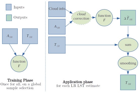
Figure 6.
Schematic representation of the downscaling methodology, on the left for the training phase, on the right the application phase.
The different parts of the methodology are evaluated in the following manner: the statistical model F is trained and tested on a different part of a large database of training samples as described in Section 3.1.3, the cloud correction is built using an independent set of data (Section 3.2). Then, the following section evaluates the performance of the methodology in an artificial clear-sky set-up only before illustrating the combined cloud correction and downscaling with a real scene.
4. Results
The downscaling methodology is tested with two different low-resolution T. In a first test, synthetic low-resolution T estimates at ∼25 km is produced by averaging the original SEVIRI IR T at ∼5 km over 5 × 5-pixel windows. This allows to evaluate the downscaling scheme independently of potential differences between the MW and IR temperatures, as it would be the case when comparing downscaled MW T with the corresponding high-resolution IR T. In addition, it makes it possible to test the methodology at different time of day as the full diurnal cycle is observed by the geostationary IR instrument (and not by a single MW polar satellite with only 2 overpass times). Illustrating scenes are shown and a global evaluation of the performance over Africa is computed. In a second test, SSMIS MW T is downscaled from its original ∼25 km to the ∼5 km of the IR ancillary information. Unlike with the previous IR clear-sky scene, the downscaling for cloudy conditions can now be illustrated as the MW T estimates are available for all weather conditions.
4.1. Downscaling of Synthetic IR Temperature
A SEVIRI T scene is selected in the south of Africa (16.7 S 21.0 E to 19.8 S 24.7 E), in the Okavango region that shows high surface heterogeneities. Sharp spatial structures are caused by the Okavango Delta with its water presence and vegetation variability also impacting the T patterns. Results are presented for two contrasted seasons and times of the day, in February (11 February 2016) at 05:00 (early morning) and in August (13 August 2016) at 12:00 (noon) respectively in Figure 7 and Figure 8 illustrating the good performance independently of the time of day of the scene.
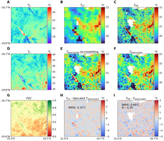
Figure 7.
Different steps of the methodology applied to a scene from 11 February 2016 at 05:00 over the Okavango Delta (16.7S 21.0E to 19.8S 24.7E). Input ancillary variables (, , ) are in the (A,D,G) panels. T at low resolution and original high resolution in the panels (B,C). The T obtained by the downscaling method, before and after smoothing in the second row (E, F). The (H) panel contains the difference between the input T and 5 × 5 average at low resolution with the RMSD overlaid over the scene. Finally, the bottom-right panel (I) shows the difference between the original high resolution and the produced by the methodology. The RMSD and the coefficient of determination (R) are overlaid on the scene.
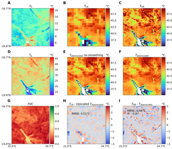
Figure 8.
Same as Figure 7, but for 13 August 2016 at 12:00.
For both figures, the three left panels (A, D, G) show the values of the ancillary variables , and . Differences in the spatial structures of the three variables are visible, with an apparent opposite behavior between and around the inner delta. This is related to the difference in heat capacity between these areas: colder minimal temperatures are associated with higher amplitude during the day. The difference in vegetation cover between the 2 selected scenes (at different seasons) is also strong.
Panel B shows the low-resolution aggregates (), with each pixel representing around km, whereas panel C displays the original T from SEVIRI (), i.e., the target T to be reproduced by the downscaling. The temperature range differs between the 2 selected times: around 20 C in the 05:00 scene, and around 40 C in the 12:00 scene. As the low-resolution values are synthetically constructed from the high-resolution ones, some are missing because of clouds contamination or invalid values (e.g., no T retrievals over water bodies). Panel E shows T after downscaling but before the smoothing step, with the final downscaled T () after smoothing displayed in panel F. The smoothing effect is apparent from the absence of block-like artifacts on the final product. Compared to the original , appears smoother with less contrast and some missing spatial structures. This can be explained by the method (averaging of contributions), F model errors, or missing data in the ancillary datasets used (e.g., around the water bodies for the February scene).
Finally, the bottom-row central and right panels (H, I) show the departure between and original . In the central panel, is spatially averaged to get a low-resolution product that can be compared to the synthetic used as input to the downscaling scheme. This shows where the downscaling procedure degrades the input temperature information. The only areas with large departures are those around places with missing data or sharp contrast between nearby pixels. The right panel displays the difference between the original and . The dark blue (red) spots are mostly around local extreme T that are regularly over(under)-estimated. This lower performance on extreme values is inherent to the neural network training scheme used to implement the F function. This scheme minimizes the squared deviation error, which leads to an underestimation of variance in the output that can sometimes be addressed with variance inflation methods [40]. Some strong errors also appear near missing values, for instance close to the water extent in the delta.
The downscaling method is further illustrated in Figure 9 where a transect along the latitude of the estimated , the targeted original , and the spatially averaged input to be downscaled are displayed. The transect integrates spatially between 12.6 N and 12.7 N, extending from 20 E to 22 E for the 18th of February/May/August/November in 2016 at 10:00. The variability shown in is clearly damped on as expected, while it is well captured in , with relatively large correlation values (coefficients of determination between 0.65 and 0.88). The applied downscaling performs equally well for a variety of temperatures between 30 C and 60 C. The already mentioned underestimation of extrema is also visible on the transect.
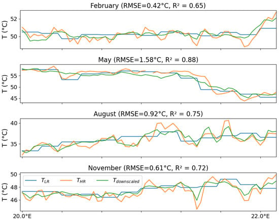
Figure 9.
Transect of the T around 12.5 N between 20 E and 22 E at 10:00 on the 18th of the months of February, May, August and November (top to bottom). For each month, the SEVIRI in orange, the 5 × 5 average in blue and the in green are shown. Also, the RMSD and coefficient of determination R between the and is displayed in each subplot title.
The previous examples show that the F function correctly reproduces the T variations at the fine scale, although it performs less well for the more extreme T values within the scenes. Overall, the downscaling produces a good approximation of the high-resolution temperatures. It also adapts well to different seasons, times of the day, and surface conditions. To quantify the performance, the Root Mean Square Deviation (RMSD) between and was computed for the 18th of the February/May/August and November months in 2016 at all hours between S– N and 22–35 E. The RMSD values range between 0.62 C in May and 1.07 C in November. The RMSD but calculated between and the spatially averaged lies between 0.74 C and 1.16 C, confirming the effectiveness of the downscaling method in producing a T estimate closer to the true T.
4.2. Downscaling of Observed SSMIS Temperature
The downscaling methodology is now applied to SSMIS MW T from the same area in the Okavango Delta. The results are presented in Figure 10. 26 November 2016 at 05:00 is selected as it presents both clear (the southern part of the scene) and cloudy conditions (the northern part, with no IR T corresponds to the cloud presence). The two panels on the left (A, D) show the ancillary variables and . Their values are different from the ones in Figure 7 and Figure 8, reflecting the seasonal changes of these variables. Please note that even if the northern part of the scene is cloudy, IR-derived and estimates still exist due to their 10-day temporal integration. Consequently, the downscaling can be applied everywhere in the scene. Panel B shows the SSMIS , i.e., the low-resolution T input to be downscaled. In panel C, the cloud correction, aggregation, and smoothing steps are applied to produce . Panel E shows the 5 × 5 averaged from SEVIRI. Finally, the original SEVIRI is shown in panel F.
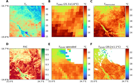
Figure 10.
For a scene from the 26th of November 2016 at 05:00 over the Okavango Delta (16.7 S 21.0 E to 19.8 S 24.7 E): the first column shows 2 of the input ancillary variables: (A) and (D). Panel (B) shows the original SSMIS () and panel (C) the , finally panel (F) shows the at high resolution and panel (E) the IR T after a 5 × 5 spatial average. The average temperature and standard deviation for the clear-sky part of the scene are indicated for and .
Comparison of original SSMIS , , and SEVIRI shows that the SEVIRI spatial structures are well captured by estimates. In the clear-sky part of the scene, correctly reproduces the north-to-south T gradient and the colder T in the riverbed, as observed on SEVIRI . The average value and standard deviation of the scene clear pixels are given for the SSMIS and SEVIRI in Figure 10, showing a warm bias of ∼1 C for SSMIS. This bias is likely related to an initial difference between the MW and IR T in this area, not to an artifact of the downscaling. For the clear-sky part of the scene, RMSD computed between the SEVIRI and SSMIS T gives values of 1.72 C with the original resolution that is improved to 1.60 C after the downscaling.
The downscaling for the cloudy part of the scene is reasonable, without any obvious artifacts compared with the clear part. The cloud correction on the variable was of the order of 3 C for this particular scene, but its impact on was not very large compared with a clear situation as the effect of on the F function is lower around the early morning hours than around midday. Comparing with SEVIRI close to the cloud edges reveals some inconsistencies. Some SEVIRI T estimates appear much colder (∼10 C) than the surrounding average T of the scene (∼20 C) and than the corresponding SSMIS estimates, suggesting a likely cloud contamination in the IR T estimates.
To better highlight the correction provided by the parameterization of the cloud effect Figure 11 shows the downscaling scheme applied to 2 consecutive days over a scene in northern Tanzania ( S 32 E to 4.9 S 35.4 E). For each day, in 2 columns, the first row (panels A, B) shows the original SSMIS T and indicates the average temperature and standard deviation over the clear-sky parts of the scene. Then the second row (C, D) shows the result after the downscaling procedure is applied. is displayed in the third row (E, F) with the average temperature and standard deviation over the scene. Finally, the last row (G, H) shows the correction on the variable that is applied based on the cloud parameterization and ERA5 data, for the cloud structure from the south-west to the north-east of the image.
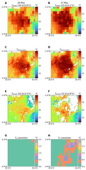
Figure 11.
Scenes from the afternoon overpass during 2 consecutive days, 26 and 27th of May 2016 over northern Tanzania ( S 32 E to 4.9 S 35.4 E): On the first line (A,B) is the SSMIS observation at low resolution, then panels (C,D) show the result after the downscaling scheme is applied, (E,F) show the at the same time. Finally, the last row (G,H) shows the correction on the parameter derived from the ERA5 reanalysis. The average and standard deviation of and for the clear-sky parts of the scene are indicated in the sub-panel titles.
Most of the cloud presence is visible in the north-east of the scene for the second day. Over the clear parts of the scene the second day is warmer than the first day, both for SSMIS and SEVIRI. The SSMIS clear-sky part of the scenes are ∼3 K warmer than the SEVIRI ones. This bias is larger than the one found in Figure 10 (∼1 K), and can be partly caused by a larger cloud contamination in due to the challenges of filtering a more broken cloud. Over a large part of the cloudy area in the second day is a bit colder, compared to the first day, possibly reflecting the impact of the cloud presence on the surface T. The illustrated correction, at the same resolution as ERA5 it is derived from, in the cloudy part of the scene reduces the of the day, with the largest correction not exceeding 2.0 C. The for both clear-sky and cloudy scenes show comparable structures, with very realistic high-resolution patterns, in agreement with the geophysical structure in this area such as the delta leading to Lake Victoria in the north-west, or the crater highland in the north-east with lower average temperatures.
5. Discussion
The previous section illustrates the performance of the methodology for the downscaling of synthetic data but also the application of the procedure to real world land-surface temperature derived from SSMIS observations. Several points arise from these results that should be taken into account when implementing such a downscaling scheme.
First, the methodology developed here is independent of the overpass time of the platform carrying the MW instruments used to derive the T. The different overpass times of each instrument (06:00 for SSMIS and 13:30 for AMSR-E for instance) are handled by the solar zenith angle factor dependence introduced in the model. The same model can therefore be applied to a low-resolution land-surface temperature product at any time of the day. This is a great benefit toward a coherent high-resolution MW-derived T product given the changing overpass times depending on the satellite missions. However, the performance of this method relies a lot on the performance of the underlying MW T, for which evaluation have been conducted for instance in [16,17,34].
Also, the ancillary variables used in the training of the F model, especially the diurnal cycle derived parameter and , offer new information sources to describe the high-resolution T patterns with a finer accuracy. This performance benefit is shown in Figure 3, and is understandable as these variables inherently summarize the thermal behavior of different surfaces. The 10-day period used in this study is a conveniently available timescale but these values could be replaced with longer time scale climatologies. For future developments outside the regions covered by geostationary satellites, MODIS T and vegetation indexes that are globally available could be used. MODIS being on board a polar orbiter with overpassing times at 01:30 and 13:30, it will not provide information over the full T diurnal cycle, but T at 01:30 is close to the minimum T and its difference with T at 13:30 can be a proxy to the amplitude of the T diurnal cycle.
The known difficulties in comparing IR and MW T over some surfaces are mitigated in this study as only the relative increase in temperatures from IR is used to infer the correction to the MW T. The training of the F model is independent from the sensor on which the methodology is applied. Of course, known limitations of the MW (over arid areas for instance) are not corrected by this methodology, but it can nevertheless improve the MW T resolution in most situations.
Finally, the correction for ancillary values under clouds developed here is not only a major building block of this methodology but is also a valuable contribution to the understanding of the expected impact of clouds on surface T. As noted in the work of [26], the assumption that clear-sky derived coefficient can also be used for cloudy scenes should be further investigated. The parameterization of the cloud effect proposed here is a first attempt to better understand what remains a high source of uncertainty in global T measurements.
6. Conclusions
To provide high-resolution ‘all-weather’ land-surface temperature, this study develops a methodology to perform a downscaling of MW-derived T, from their original spatial resolution of ∼25 km to a resolution of ∼5 km, similar to IR geostationary observations.
To that end, a statistical relationship is first established between high-resolution ancillary information and high-resolution T, to estimate the T fine spatial resolution patterns under clear-sky conditions. The model is trained using IR T and ancillary products from IR SEVIRI geostationary observations at ∼5 km. Different combinations of variables are tested and the model error is lowest over the whole range of temperature, using the minimal value and the amplitude of the median clear-sky temperature diurnal cycle ( and ), along with the fractional vegetation cover , and the solar elevation angle (). In an application phase, the statistical function is then used to produce a high-resolution temperature pattern that is added to the coarse resolution T and provides spatially finer T estimates.
To test the methodology under clear-sky conditions, the original ∼5 km T estimates are used as the fine resolution T, with the coarse resolution T synthetically produced from aggregation of the original T to a ∼25 km resolution. The RMSD of the downscaled T against the high-resolution one remains below 1 C for a variety of conditions (spanning multiple months and all hours of day), showing the possibility to correctly reproduce the original T with this method. For cloudy scenes, the same statistical function is used, but with a prior reduction of the input to account for the cloudy conditions. This correction is based on an analysis of the average impact of clouds on T using cloud information from ECMWF ERA5 reanalysis. Finally, the downscaling and cloud correction performance are tested on an original SSMIS-derived land-surface temperature scene at ∼25 km resolution, and the resulting downscaled scene at ∼5 km is compared to the nearly coincident SEVIRI-derived estimates. The RMSD over the clear-sky part of the scene and the original low-resolution is 1.72 C and is reduced to 1.60 C after downscaling. The downscaling could not be tested under cloudy conditions as no high-resolution satellite product is yet available for cloudy scenes.
The results demonstrate the relevance of the methodology to perform the downscaling of MW land-surface temperature, with an adaptability to seasons and times of the day, along with a specific handling of the cloudy areas. The required inputs are limited, keeping the implementation of the method rather simple. The method can already be used for all areas for which the geostationary satellites data is available, including the often-cloudy tropical areas. Additional study could be performed to evaluate the possibility to generalize the predictors for a global downscaling, for instance using polar orbiting high-resolution IR sensors. These data sources would also provide an opportunity to downscale the MW T to a higher resolution, up to ∼1 km.
This is the first step toward the application of a generic methodology to downscale the ∼40 years of MW-derived land-surface temperature currently under production [29]. It will provide an ‘all-weather’ climatology of land-surface temperature at global scale with a high spatial resolution, to complement the clear-sky only IR estimates.
Author Contributions
Data collection and preliminary work, conception and data analysis have been conducted by S.F., C.P., C.J. and S.F. wrote and edited the final manuscript. All authors have read and agreed to the published version of the manuscript.
Funding
This research was funded by the European Space Agency under the Climate Change Initiative, Essential Climate Variables Land-Surface Temperature project with contract n 4000123553/18/I-NB. Funding was also granted by the Agence Nationale Recherche Technologie, with the CIFRE n 2018/0637.
Institutional Review Board Statement
Not applicable.
Informed Consent Statement
Not applicable.
Data Availability Statement
All data used in this study is freely available from the sources mentioned in the Data section.
Acknowledgments
The authors are grateful to Sofia Ermida from Instituto Portugues do Mar e da Atmosfera, Lisbon, for the information on the cloud effect on temperatures, as well as Filipe Aires from Observatoire de Paris, for the discussions regarding the formalism in the downscaling methodology. The various reviewers contributions was also very helpful in crafting the final manuscript version.
Conflicts of Interest
The authors declare no conflict of interest.
References
- Bojinski, S.; Verstraete, M.; Peterson, T.C.; Richter, C.; Simmons, A.; Zemp, M. The concept of essential climate variables in support of climate research, applications, and policy. Bull. Am. Meteorol. Soc. 2014, 95, 1431–1443. [Google Scholar] [CrossRef]
- Bechtel, B. A new global climatology of annual land surface temperature. Remote Sens. 2015, 7, 2850–2870. [Google Scholar] [CrossRef]
- Wan, Z.; Dozier, J. Land-Surface Temperature Measurement from Space: Physical Principles and Inverse Modeling. IEEE Trans. Geosci. Remote Sens. 1989, 27, 268–278. [Google Scholar] [CrossRef]
- Trigo, I.F.; Peres, L.F.; DaCamara, C.C.; Freitas, S.C. Thermal land surface emissivity retrieved from SEVIRI/Meteosat. IEEE Trans. Geosci. Remote Sens. 2008, 46, 307–315. [Google Scholar] [CrossRef]
- Wan, Z.; Li, Z.L. A physics-based algorithm for retrieving land-surface emissivity and temperature from eos/modis data. IEEE Trans. Geosci. Remote Sens. 1997, 35, 980–996. [Google Scholar] [CrossRef]
- Ermida, S.L.; Trigo, I.F.; DaCamara, C.C.; Jiménez, C.; Prigent, C. Quantifying the Clear-Sky Bias of Satellite Land Surface Temperature Using Microwave-Based Estimates. J. Geophys. Res. Atmos. 2019, 124, 844–857. [Google Scholar] [CrossRef]
- Jin, M. Interpolation of surface radiative temperature measured from polar orbiting satellites to a diurnal cycle: 2. Cloudy-pixel treatment. J. Geophys. Res. Atmos. 2000, 105, 4061–4076. [Google Scholar] [CrossRef]
- Martins, J.P.; Trigo, I.F.; Ghilain, N.; Jimenez, C.; Göttsche, F.M.; Ermida, S.L.; Olesen, F.S.; Gellens-Meulenberghs, F.; Arboleda, A. An all-weather land surface temperature product based on MSG/SEVIRI observations. Remote Sens. 2019, 11, 3044. [Google Scholar] [CrossRef]
- Wu, P.; Yin, Z.; Zeng, C.; Duan, S.B.; Gottsche, F.M.; Li, X.; Ma, X.; Yang, H.; Shen, H. Spatially Continuous and High-Resolution Land Surface Temperature Product Generation: A Review of Reconstruction and Spatiotemporal Fusion Techniques. IEEE Geosci. Remote Sens. Mag. 2021. [Google Scholar] [CrossRef]
- Xu, S.; Cheng, J. A new land surface temperature fusion strategy based on cumulative distribution function matching and multiresolution Kalman filtering. Remote Sens. Environ. 2021, 254, 112256. [Google Scholar] [CrossRef]
- Wu, P.; Yin, Z.; Yang, H.; Wu, Y.; Ma, X. Reconstructing geostationary satellite land surface temperature imagery based on a multiscale feature connected convolutional neural network. Remote Sens. 2019, 11, 300. [Google Scholar] [CrossRef]
- McFarland, M.; Miller, R.; Neale, C. Land surface temperature derived from the SSM/I passive microwave brightness temperatures. IEEE Trans. Geosci. Remote Sens. 1990, 28, 839–845. [Google Scholar] [CrossRef]
- Weng, F.; Grody, N.C. Physical retrieval of land surface temperature using the special sensor microwave imager. J. Geophys. Res. Atmos. 1998, 103, 8839–8848. [Google Scholar] [CrossRef]
- Aires, F.; Prigent, C.; Rossow, W.B.; Rothstein, M. A new neural network approach including first guess for retrieval of atmospheric water vapor, cloud liquid water path, surface temperature, and emissivities over land from satellite microwave observations. J. Geophys. Res. Atmos. 2001, 106, 14887–14907. [Google Scholar] [CrossRef]
- Holmes, T.R.H.; De Jeu, R.A.M.; Owe, M.; Dolman, A.J. Land surface temperature from Ka band (37 GHz) passive microwave observations. J. Geophys. Res. Atmos. 2009, 114, 1–15. [Google Scholar] [CrossRef]
- Jiménez, C.; Prigent, C.; Ermida, S.L.; Moncet, J.L. Inversion of AMSR-E observations for land surface temperature estimation: 1. Methodology and evaluation with station temperature. J. Geophys. Res. 2017, 122, 3330–3347. [Google Scholar] [CrossRef]
- Ermida, S.L.; Jiménez, C.; Prigent, C.; Trigo, I.F.; DaCamara, C.C. Inversion of AMSR-E observations for land surface temperature estimation: 2. Global comparison with infrared satellite temperature. J. Geophys. Res. 2017, 122, 3348–3360. [Google Scholar] [CrossRef]
- Kustas, W.P.; Norman, J.M.; Anderson, M.C.; French, A.N. Estimating subpixel surface temperatures and energy fluxes from the vegetation index-radiometric temperature relationship. Remote Sens. Environ. 2003, 85, 429–440. [Google Scholar] [CrossRef]
- Zhan, W.; Chen, Y.; Zhou, J.; Wang, J.; Liu, W.; Voogt, J.; Zhu, X.; Quan, J.; Li, J. Disaggregation of remotely sensed land surface temperature: Literature survey, taxonomy, issues, and caveats. Remote Sens. Environ. 2013, 131, 119–139. [Google Scholar] [CrossRef]
- Merlin, O.; Walker, J.P.; Chehbouni, A.; Kerr, Y. Towards deterministic downscaling of SMOS soil moisture using MODIS derived soil evaporative efficiency. Remote Sens. Environ. 2008, 112, 3935–3946. [Google Scholar] [CrossRef]
- Peng, J.; Loew, A.; Merlin, O.; Verhoest, N.E. A review of spatial downscaling of satellite remotely sensed soil moisture. Rev. Geophys. 2017, 55, 341–366. [Google Scholar] [CrossRef]
- Aires, F.; Prigent, C.; Rossow, W.B. Temporal interpolation of global surface skin temperature diurnal cycle overland under clear and cloudy conditions. J. Geophys. Res. Atmos. 2003, 109. [Google Scholar] [CrossRef]
- Göttsche, F.M.; Olesen, F.S. Modelling the effect of optical thickness on diurnal cycles of land surface temperature. Remote Sens. Environ. 2009, 113, 2306–2316. [Google Scholar] [CrossRef]
- Duan, S.B.; Li, Z.L.; Leng, P. A framework for the retrieval of all-weather land surface temperature at a high spatial resolution from polar-orbiting thermal infrared and passive microwave data. Remote Sens. Environ. 2017, 195, 107–117. [Google Scholar] [CrossRef]
- Sun, D.; Li, Y.; Zhan, X.; Houser, P.; Yang, C.; Chiu, L.; Yang, R. Land surface temperature derivation under all sky conditions through integrating AMSR-E/AMSR-2 and MODIS/GOES observations. Remote Sens. 2019, 11, 1–20. [Google Scholar] [CrossRef]
- Zhang, X.; Zhou, J.; Gottsche, F.M.; Zhan, W.; Liu, S.; Cao, R. A Method Based on Temporal Component Decomposition for Estimating 1-km All-Weather Land Surface Temperature by Merging Satellite Thermal Infrared and Passive Microwave Observations. IEEE Trans. Geosci. Remote Sens. 2019, 57, 4670–4691. [Google Scholar] [CrossRef]
- Schmid, J. The SEVIRI instrument. In Proceedings of the 2000 EUMETSAT Meteorological Satellite Data User’s Conference, Bologna, Italy, 29 May–2 June 2000. [Google Scholar]
- Hersbach, H.; Bell, B.; Berrisford, P.; Hirahara, S.; Horányi, A.; Muñoz-Sabater, J.; Nicolas, J.; Peubey, C.; Radu, R.; Schepers, D.; et al. The ERA5 global reanalysis. Q. J. R. Meteorol. Soc. 2020, 146, 1999–2049. [Google Scholar] [CrossRef]
- Consortium CCI LST. Algorithm Theoretical Basis Document WP2.1 – DEL-LST-CCI-D2.2-ATBD. 2019. Available online: https://climate.esa.int/sites/default/files/LST-CCI-D2.2-ATBD%20-%20i1r1%20-%20Algorithm%20Theoretical%20Basis%20Document.pdf (accessed on 31 March 2021).
- Perry, M.; Ghent, D.; Jimenez, C.; Dodd, E.; Ermida, S.L.; Isabel, F. Multi-Sensor thermal infrared and microwave land surface temperature algorithm intercomparison. Remote Sens. 2020, 12, 4164. [Google Scholar] [CrossRef]
- Trigo, I.F.; Dacamara, C.C.; Viterbo, P.; Roujean, J.L.; Olesen, F.; Barroso, C.; Camacho-De-Coca, F.; Carrer, D.; Freitas, S.C.; García-Haroj, J.; et al. The satellite application facility for land surface analysis. Int. J. Remote Sens. 2011, 32, 2725–2744. [Google Scholar] [CrossRef]
- García-Haro, F.; Camacho, F.; Meliá, J. The EUMETSAT Satellite Application Facility on Land Surface Analysis Product User Manual Vegetation Parameters ( VEGA ). EUMETSAT Prod. User Man. 2013, 401, 1–46. [Google Scholar]
- Johannsen, F.; Ermida, S.; Martins, J.P.; Trigo, I.F.; Nogueira, M.; Dutra, E. Cold bias of ERA5 summertime daily maximum land surface temperature over Iberian Peninsula. Remote Sens. 2019, 11, 2570. [Google Scholar] [CrossRef]
- Prigent, C.; Jimenez, C.; Aires, F. Toward “all weather,” long record, and real-time land surface temperature retrievals from microwave satellite observations. J. Geophys. Res. 2016, 121, 5699–5717. [Google Scholar] [CrossRef]
- Rumelhart, D.E.; Hinton, G.E.; Williams, R.J. Learning representations by back-propagating errors. Nature 1986, 323, 533–536. [Google Scholar] [CrossRef]
- Hornik, K. Approximation capabilities of multilayer feedforward networks. Neural Netw. 1991, 4, 251–257. [Google Scholar] [CrossRef]
- Chen, T.; Rossow, W.B.; Zhang, Y. Radiative effects of cloud-type variations. J. Clim. 2000, 13, 264–286. [Google Scholar] [CrossRef]
- Friedl, M.; Strahler, A.; Hodges, J. ISLSCP II MODIS (Collection 4) IGBP Land Cover, 2000–2001; ORNL DAAC: Oak Ridge, TN, USA, 2010. [Google Scholar] [CrossRef]
- Aires, F.; Miolane, L.; Prigent, C.; Pham, B.; Fluet-Chouinard, E.; Lehner, B.; Papa, F. A global dynamic long-term inundation extent dataset at high spatial resolution derived through downscaling of satellite observations. J. Hydrometeorol. 2017, 18, 1305–1325. [Google Scholar] [CrossRef]
- Von Storch, H. On the use of ’inflation’ in statistical downscaling. J. Clim. 1999, 12, 3505–3506. [Google Scholar] [CrossRef]
Publisher’s Note: MDPI stays neutral with regard to jurisdictional claims in published maps and institutional affiliations. |
© 2021 by the authors. Licensee MDPI, Basel, Switzerland. This article is an open access article distributed under the terms and conditions of the Creative Commons Attribution (CC BY) license (https://creativecommons.org/licenses/by/4.0/).