Automatic Cotton Mapping Using Time Series of Sentinel-2 Images

Abstract

Large-scale crop mapping is essential for agricultural management. Phenological variation often exists in the same crop due to different climatic regions or practice management, resulting in current classification models requiring sufficient training samples from different regions. However, the cost of sample collection is more time-consuming, costly, and labor-intensive, so it is necessary to develop automatic crop mapping models that require only a few samples and can be extended to a large area. In this study, a new white bolls index (WBI) based on the unique canopy of cotton at the bolls opening stage was proposed, which can characterize the intensity of bolls opening. The value of WBI will increase as the opening of the bolls increases. As a result, the white bolls index can be used to detect cotton automatically from other crops. Four study areas in different regions were used to evaluate the WBI performance. The overall accuracy (OA) for the four study sites was more than 82%. Additionally, the dates when the opening stage of bolls begins can be determined based on the time series of WBI. The results of this research demonstrated the potential of the proposed approach for cotton mapping using sentinel-2 time series of remotely sensed data.

1. Introduction

Agriculture is the main contributor to the global economy, food security, and ecological environment and provides grain, non-staple food, and industrial raw materials for human beings [1,2,3]. Cotton is one of the world’s most important fiber crops for the economy, supplying some 79% of the world’s natural fiber and expanding one of the largest textile industries to at least $600 billion annually worldwide [4,5,6]. More than 100 cotton-producing countries worldwide are planting the total area for cotton production in 2014 is 33 M ha for the entire world. Of these, India, China, the United States, Pakistan, Brazil, Australia, Uzbekistan, Turkey, Turkmenistan, and Burkina Faso are among the top ten cotton-producing countries [6]. Different cotton variations have been developed, for example, the genetic engineering Bacillus thuringiensis (Bt), which rapidly increases cotton production [7]. Therefore, it is necessary to automatically map cotton distribution for wide scales in time to match the significantly accelerated breeding process.

Satellite Image Time Series (SITS) have been widely used to identify crops in large regions because of their global coverage and short revisit periods to capture canopy coverage of crops at various growth stages [8,9,10,11]. As one crop type, cotton can be mapped with crop classification technologies based on remote sensing images.

Generally, there are two steps for classification technologies. Firstly, the time-series features of original spectral bands [12] or vegetable indexes [13,14,15] are extracted, such as the statistical characteristic [16,17,18] such as mean, variance, maximum values, transformed components, etc. and phenological features [19,20,21,22,23,24] such as the start of greening/season, the peak of the season, the end of the season, fitted curve parameter, and so forth. Secondly, training samples train the classification models with the features above. The most widely used classifiers including random forest (RF), decision tree (DT), support vector machine (SVM), K-nearest neighbor (KNN), and the advance deep learning models [25,26,27]. Then, the trained models can predict the crop classes.

As is well known, due to the different climatic regions or practice management, there are phenological diversities within the same crops [28], which lead the trained models with samples of the old region to unfit the new regions. Updating the training samples can solve this problem, but it is more time-consuming, costly, and labor-intensive. Recently, several studies have explored unique phenological characteristics to automatically map crops without the amount of training data. For example, Ashourloo et al. (2018) developed a new feature for the identification of alfalfa with the phenological patterns of alfalfa from a multi-harvest one-year time series of Landsat 8 data, which detected alfalfa with the overall accuracy being better than 90% [29]. Qiu et al. (2017) found that the length of growth period in winter wheat was longer than that in other crops, based on which a temporal index within an EVI time series was developed to map winter wheat [30]. Recently, several studies derived the identification characteristics of the crop canopy in a certain phenological stage to map the crops. For example, Andrimont et al. (2020) utilized a yellow flower index in the flowering stage to detect canola [31]. Ashourlooa et al. (2019) developed a Canola Index to characterize the yellow flower and automatically map the canola [32].

Observations from previous studies indicate that most crops display a particular phenological or canopy pattern in a certain phenological stage. In comparison with the phenological patterns, canopy patterns are bound to occur at a certain date, even if under different climatic regions or practice managements. Hence, it is a better way to automatically map crops with the unique canopy feature.

Similar to the yellow canola flowers in the flowering period, cotton also has the distinctive trait of the canopy that current research studies pay less attention to. The stages covering cotton growing are planted (when the seeds are placed in the ground), squaring (when the appearance of a small triangular leaf-like structure on the growing tip of the main stem and/or branches), setting bolls (when one bloom or boll is visible), bolls opening (when white fibers are visible on at least one boll), and harvested (when the cotton is cut or gathered from the field) [33]. Cotton is known as “white gold” in some countries [34], which vividly describes the characteristic of the cotton canopy in the bolls opening stage. Since bolls are full of white wool, the cotton canopy appears white, which is a distinctive trait and different from other crops.

In this research, a white bolls index (WBI) that characterizes the intensity of bolls opening during cotton growing is constructed with few training samples. With the increase of the bolls opening, the value of WBI will be larger and vice versa. Based on the feature of the WBI, it can be used to map cotton under various cultivations and climate areas without training samples. Additionally, the date that the bolls opening stage begins can be recognized by the WBI time series.

The rest of the paper is organized as follows. The material and methods of the study are described in Section 2. Results and discussion are respectively presented in Section 3 and Section 4. The last Section 5 provides conclusions of the study.

2. Materials and Methods

Figure 1 shows the summary of the research stages and flowchart of this study. Firstly, 4 study sites were described and datasets including satellite image time series with ground references were presented. Then, the WBI of cotton was constructed based on temporal–spectral conjoint analysis with training samples. Thirdly, cotton was mapped in the 4 study sites with the empirical threshold method. Fourthly, the start date of the bolls opening stage was derived from the WBI time series based on the cotton maps. At last, we evaluated the classification results with test samples and the start of bolls opening date with the phenological data from United States Department of Agriculture National Agricultural Statistics Service (USDA-NAS) and ground survey.

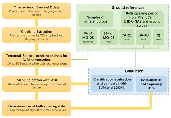
Figure 1. Flowchart of the current study for automatic mapping of cotton.

2.1. Study Sites

Four study sites were chosen to test the proposed index under different environmental conditions. These included Missouri’s 8th District (MO-08), California’s 21st District (CA-21), Georgia’s 8th District, and Shihezi and its surrounding areas (Shihezi reclamation area) in China’s North Xinjiang (XJ). All of the 4 study sites are mechanical cultivation, including sowing, fertilization, irrigation, weed removal, and insect management in the cotton growth period. Additionally, defoliation should proceed to ensure optimum yield and fiber quality. However, the specific practice that should be performed depends on the field situation. The cotton planting area ranges from smaller to larger in these areas. These areas, which have various agro-climatic conditions, climates, and crop types, are situated from west to east. The location of the study sites is shown in Figure 2, and the climatological and agricultural conditions at each site are shown in Table 1.

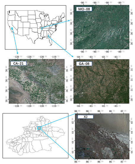
Figure 2. Study sites.

Table 1. Climatological and agricultural characteristics of different sites.

Region	Elevation (m)	Average Temperature (°C)	Precipitation (mm)	Climate Classification	Major Crop Type	Rank of Cotton in State and U.S.	Major Cotton Type
MO-08	83	15.27	1399.03	Dfa	soybean, cotton, rice, corn	1/10	Upland
CA-21	32	15.05	489.20	Csb	almonds, grapes, cotton, pistachios	1/4	PIMA
GA-08	60	19.88	1492.50	Cfa	cotton, peanuts, corn	2/9	Upland
XJ	347	7.41	221.44	BWk	cotton, wheat, corn	--	Upland

Dfa: Snow climate, fully humid, Hot summer Csb: Warm temperate climate with dry summer, Warm summer Cfa: Warm temperate, fully humid, Hot summer BWk: Arid climate, desert, cold arid.

MO-08 is one of eight congressional districts in the state of Missouri. The district encompasses rural Southeast Missouri and South Central Missouri as well as some counties in Southwest Missouri. Cotton in Dunklin and Stoddard counties rank in the top 3 in MO state. Hence, these 2 counties were selected for the study site. Other major crops contain soybean, rice, and corn. Cotton is planted in late May, the bolls open in mid to late September, and are harvested in mid to late October and early November. Figure 3 showed the phenological stages of cotton nearby the study site from the ecosystem phenology camera network (PhenoCam) (https://phenocam.sr.unh.edu/webcam/ (accessed on 1 March 2021).

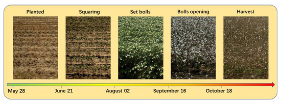
Figure 3. The phenological stages of cotton nearby MO-08.

CA-21 is a congressional district in the U.S. state of California. It is located in the San Joaquin Valley and includes Kings County and portions of Fresno, Kern, and Tulare counties. This paper selected Fresno and Kings as the main study areas, since more cotton was planted here than in other counties. Cotton is the second major crop in CA-21, while the first major crop is fruit trees. There are various fruit trees, such as almonds, grapes, pistachios, and so on. Cotton in CA-21 is planted in late April, the stage of bolls opening starts in late September and early October, and then, cotton is harvested in mid to late November.

GA-08 is one of the congressional districts in the U.S. state of Georgia. Our study site here including 9 counties, half of which rank in the top 10 in planting cotton. There are other major crops here, such as peanuts and corn. Cotton in GA-08 is planted in late April, the stage of bolls opening starts in late September and early October, and cotton is harvested after middle November.

Xinjiang is the biggest cotton-growing province in China, where 36% of cropland is cotton. The reclamation area of Shihezi is one of the major production bases for high-quality cotton in Xinjiang, where 70% of cropland is covered by cotton. Hence, it is selected as the study site, and other crops include wheat, corn, and fruit trees. Cotton here is planted from early to mid April, bolls are opening from late August to early September, and cotton is harvested in late October.

2.2. Data Used in the Study

2.2.1. Satellite Images

Time series of Sentinel-2 images covering the study sites from April to November 2019 were used to train the white bolls index. Cloud percentage was limited to less than 10%. The corresponding years and Julian’s days are shown in Table 2. As can be seen in Table 2, CA-21 has the most images, with a total of 39 scenes; MO-08, GA-08, and XJ had 20, 11, and 22 scenes respectively. Ten bands were used to extract white bolls index, including B2(Blue), B3(Green), B4(Red), B5(RedEdge1), B6(RedEdge2), B7(RedEdge3), B8(NIR), B8A(narrow NIR or RedEdge4), B11(SWIR1), and B12(SWIR2) from Google Earth Engine (GEE) surface reflectance products with 10,000 scale.

Table 2. Sentinal-2 time series used in study areas.

Region	Year	Tile NO.	Julian Days
MO-08	2019	15SYA	106 111 116 136 151 161 181 206 231 241 246 256 261 276 281 286 291 296 306 331
CA-21	2019	10SGF	97 102 107 112 122 127 132 152 157 167 172 177 182 187 192 197 202 207 212 222 227 232 237 242 247 252 257 262 267 272 277 282 287 297 302 307 312 322 327
GA-08	2019	17RKQ	112 117 127 147 242 262 267 277 307 317 332
XJ	2019	45TVK	104 129 149 159 164 179 184 199 209 214 219 224 239 244 254 264 279 284 289 299 304 309

Surface reflectance products were computed by running sen2cor on level-1C products. B2, B3, B4, and B8 are 10 m resolution, which was resampled to 20 m with bilinear algorithm from GEE. Additionally, temporal interpolation was applied to remove clouds from the time series. The 20 m surface reflectance time series with the free cloud can be obtained through the above pre-processing.

2.2.2. Ground References

Crop types of 2058 fields located in the 4 study sites of MO-08 (851 fields), CA-21 (734 fields), GA-08 (254 fields), and XJ (219 fields) were collected. In MO-08, 239, 244, 187, 152, and 29 field samples for cotton, soybean, corn, rice, and peanuts were included in the collected dataset. In CA-21, 159, 415, 59, 57, and 44 field samples were included for cotton, fruit trees (grape, almond, pistachio, walnut), corn, rice, and peanuts. In GA-08, there were 159, 42, 14, and 39 field samples for cotton, peanuts, pecans, and corn. In XJ, there were 122 and 97 field samples for cotton and other crops including corn, grapes, wheat, and sorghum. The size of the fields in the study areas was very different and varies between 0.3 and 50 ha.

The U.S. ground cotton phenological stages are from PhenoCam and the United States Department of Agriculture National Agricultural Statistics Service (USDA-NAS). Filed investigation, meteorological stations, and references [35,36] were used to derive the ground phenological stages in XJ.

Table 3 shows the training and test samples. Of these, 5% of the samples from 851 field samples of MO-08 were used as training to construct the WBI. The rest of the samples were left to test the model. The reflectance of samples during all the growth periods was analyzed to produce the white bolls index.

Table 3. Training and test samples used in four study areas.

Crop Name		MO-08		CA-21		GA-08		XJ
		Training	Test	Training	Test	Training	Test	Training	Test
Cotton	Cotton	12	227	0	159	0	159	0	122
Other crops	Soybean	12	232	--	--	--	--	0	97
	Corn	9	178	0	59	0	39
	Rice	8	144	0	57	--	--
	Peanuts	3	26	0	44	0	42
	Fruit trees	--	--	0	415	--	--
	Pecans	--	--	--	--	0	14

2.3. Method

2.3.1. Temporal and Spectral Conjoint Analysis

The time series of Sentinel data was used to study the reflectance values of cotton and other crops during the period from planting time to harvesting time. The training site is MO-08, where the growth period of cotton is similar to corn, sorghum, soybean, rice, and peanuts. Figure 4 shows the normalized difference vegetation index (NDVI) of various crops. As is shown in Figure 4, cotton, peanuts and rice have almost the same cultivating date, which is difficult to recognize only based on NDVI.

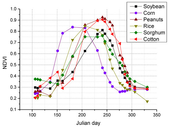
Figure 4. Normalized difference vegetation index (NDVI) time series of various crops in MO-08.

As is well known, the color of most crops’ canopy always turns yellow from green during the growth period. However, cotton has a unique feature in the canopy by comparing with other crops, which is that the color of the canopy will turn white at the stage of bolls opening. The unique white bolls of cotton can provide the clue for automatically detecting cotton from others.

To extract the characteristic of white bolls, the training samples should be divided into 2 classes: white bolls (class C, including the bolls opening stage of cotton) and others (class O, including other crops and other phenological stages of cotton). According to USDA-NAS, the bolls always open in mid to late September, and the cotton harvests at mid to late October and early November in MO; therefore, Julian’s days from 261 (September 18) to 291 (October 18) were selected as the bolls opening stage. The scatter plot of the reflectance in different temporal images was graphed in Figure 5.

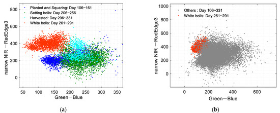
Figure 5. (a) The scatter plot of cotton in bolls opening stage and other phenological stages. (b) The scatter plot of white bolls and other crops (corn, sorghum, soybean, rice, and peanuts) from the planting stage to the harvesting stage.

Blue, Green, RedEdge3, and narrow NIR bands were combined to demonstrate the distinctions between white bolls and others. Figure 5a showed various phenological stages of the cotton. On day 261~291 of the bolls opening stage, the spectral scatter points gathered in the top-left corner, and most of the points are smaller than 200 in the X-direction and larger than 300 in the Y-direction. The points in other phenological stages of cotton, including planted, squaring, setting bolls, and harvested (the color of the canopy is brown, green, and brown in turn) are distributed larger than 100 in the X-direction and smaller than 400 in the Y-direction. Similarly, Figure 5b showed the same distribution, where non-cotton crops such as corn, sorghum, soybean, rice, and peanuts are presented by the gray points on day 106~331.

The analysis of reflectance in different dates above shows that Sentinel-2 time series are potentially used to extract the white bolls of cotton.

2.3.2. Discriminate the Cotton Bolls from Other Crops

To find the optimal index representing the characteristic of white bolls, the first step is maximizing the discrepancy between the reflectance values of white bolls (class C) and others (class O). The second step is constructing the white bolls index, indicating the number of white bolls. The larger the index value is, the more the bolls open up.

In the first step, linear discriminant analysis (LDA) [37] is used to separate the white bolls from others:

$$\underset{w}{\max }\hspace{0.17em}\frac{w^T{S}_{b}w}{w^T{S}_{w}w}$$

(1)

where S_b is the between-class scatter matrix, S_w is the within-class scatter matrix, and w is the transformation matrix. S_b and S_w are related to the samples’ reflectance of class C and class O. After the optimizing procedure, the optimal w can be obtained. The transformation reflectance can lead to the max discrepancy between class O and class C:

$$P=w^{T}R$$

(2)

where R = [r₁,r₂,…,r_n]^T is the reflectance of one sample, and P = [p₁,p₂,…,p_n]^T is the transformed reflectance.

In the second step, the index indicating the number of opening bolls was constructed by a function, the value of which can change with the intensity of opening bolls:

$$White\hspace{0.17em}Boll\hspace{0.17em}index\hspace{0.17em}(WBI)=f(p_1,p_2,\dots ,p_n)$$

(3)

where f(x) is the function of the transformed reflectance.

2.3.3. Compared with Supervised Classifier

To evaluate the potential of the proposed index, two popular classifiers were compared, namely SVM and 1-dimensional convolutional neural network (1DCNN). SVM is a non-parametric classifier with no assumption about the distribution of underlying data. Recently, SVM has been conducted in the remote sensing community in many studies [38,39]. The code we used is from module sklearn.svm.

Deep learning models were developed for land cover classification these years, which leads to very high accuracy. 1DCNN was the most popular model for a crop classification-based satellite time series [25,40]. The code we used is from git-hub bhavesh907-Crop-Classification.

In this paper, all the algorithms, including WBI, SVM, and 1DCNN were trained by the same training samples and predicted for the same test samples (as Table 3 shows). Due to the number of images in various study sites being different, SVM and 1DCNN models trained by MO-08 can not predict other sites. Therefore, we selected the same number of images with near dates from the study sites, trained SVM and 1DCNN with MO-08, and then predicted other sites. We categorized training and test data into two classes of cotton and other crops. The overall accuracy and kappa coefficient are used to evaluate the results.

2.3.4. Extract the Start of Bolls Opening Time

Based on the white bolls index time series, the start date of the bolls opening can be extracted based on the phenological algorithm. The WBI time series should be filtered by Savitzky–Golay [41] to remove the noises, and the start of season time (SOS) can be detected as the bolls opening date, due to the value of WBI starting to increase with the bolls opening.

Midpoint [42] was applied to extract SOS from the WBI series. The threshold of SOS is determined as the 50% of the VI amplitude, and the ratio can be computed as follows:

$$V{I}_{ratio}=\frac{VI-V{I}_{\min }}{V{I}_{\max }-V{I}_{\min }}$$

(4)

where VI_max is the maximum value of the WBI time series, and VI_min is the minimum value of the WBI time series. VI is the current value of the WBI time series.

3. Results

3.1. Construction of White Bolls Index

In this study, LDA was used to separate the white bolls from others. Optimizing Equation (1), the transformation matrix w^T can be obtained as shown in Equation (5).

$$w=S_w^{-1}({\mu }_0-{\mu }_1)$$

(5)

where u_j corresponds to the mean value of class j. With the LDA transformation, white bolls and others were maximum separated. Figure 6 showed the scatter plot of the first two transformed reflectances, namely LDA1 and LDA2.

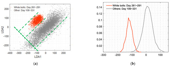
Figure 6. (a) Scatter plot for white bolls and others (including cotton in other stages, corn, sorghum, soybean, rice, and peanuts in growth period) based on LDA1 and LDA2. (b) The histogram of the projected points in (a) along the green line, which shows the separation degree between white bolls and others.

As shown in Figure 6, the values of white bolls were centered in −200 and other crops concentrated in 0 in the projected direction. The white bolls index can be constructed based on the first two LDA components. Several combinations of the two LDA bands were tried for the separation of white bolls from other crops. Figure 7 showed the box plot for different combinations.

Figure 7. The value distribution for white bolls and other crops with four combinations of linear discriminant analysis (LDA) components. p₂ × p₁, p₂ + p₁, p₂ − p₁, (p₂ − p₁)^2.

Based on Figure 7, the combination p₂ − p₁ showed the highest separation potential for the identification of white cotton bolls from others. Therefore, the white bolls’ index was proposed as follows:

$$\begin{array}{ll}\mathrm{White}\hspace{0.17em}\mathrm{bolls}\hspace{0.17em}\mathrm{index}& \left(\mathrm{WBI}\right)=1.07 \times blue - 0.68\times green - 0.24 \times red+0.17 \times R{E}_1 - 0.04 \times R{E}_2\\ & 0.39 \times R{E}_3 + 0.04 \times NIR + 0.36 \times NI{R}_{narrow} - 0.01 \times SWI{R}_1 - 0.04 \times SWI{R}_2\end{array}$$

(6)

The WBI values for different crops on Julian’s days 106~331 in the study sites were shown in Figure 8. During the stage of bolls opening (day 261–291), the mean WBI values are obviously larger than those of other crops, while the WBI values of other crops are always lower than 100 in all growing stages, and those of white bolls are far higher than 100. The significant differences of WBI between cotton and other crops can acceptably detect cotton from other crops.

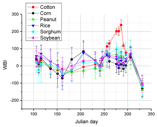
Figure 8. White bolls index (WBI) values for different crops on day 106–331.

3.2. Automatically Mapping the Cotton with White Bolls Index and Accuracy Assessment

In several remote sensing studies, empirical methods have been successfully employed for threshold determination [21,29], which was used in this study to select acceptable threshold values. We used the training samples in MO to measure the kappa coefficients at various thresholds. According to Figure 7, the range of thresholds is set from 70 to 270 and the search step is 10. Figure 9 shows that the best accuracy occurs between 100 and 220 of the WBI value, which is an acceptable threshold for detecting cotton from other crops. Additionally, before using the threshold to map cotton, it is better to mask the non-cropland to avoid interference from other ground objectives with white color.

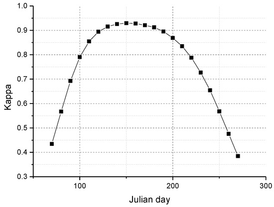
Figure 9. Kappa coefficients for mapping cotton under different thresholds.

Table 4 displays the accuracy of classification based on WBI, SVM, and 1DCNN. The models were trained by the same samples of MO-08 and applied to test samples of MO-08 and other study sites (CA-21, GA-08, and XJ). As the table shows, SVM and 1DCNN can produce very high precision in MO-08, reaching 97% above, but they offer a lower output in CA-21, GA-08, and XJ than WBI. The best results are shown by the bold fonts.

Table 4. Accuracy of cotton classification based WBI, support vector machine (SVM), and one-dimensional convolutional neural network (1DCNN).

Study Site	SVM		1DCNN		WBI
	OA	Kappa	OA	Kappa	OA	Kappa
MO-08	0.99	0.98	0.99	0.99	0.97	0.92
CA-21	0.83	0.56	0.76	0.16	0.90	0.74
GA-08	0.70	0.43	0.41	0.01	0.83	0.67
XJ	0.59	0.29	0.27	0.10	0.95	0.88

Figure 10 illustrates the derived cotton maps of the four study sites. The background is the true color composite by R, G, and B bands.

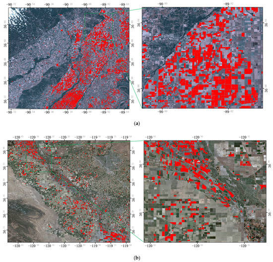
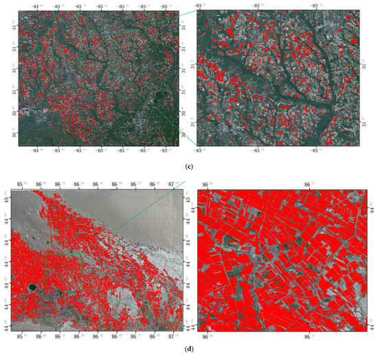
Figure 10. The derived cotton maps in (a) MO-08, (b) CA-21, (c) GA-08, and (d) XJ.

3.3. Identification of Bolls Opening Date

The window of the SG filter is set to 5~11, and the ratio is set to 0.5. The SOS of the WBI series can be seen as the bolls opening date. Figure 11 shows the procedure of the extraction for the bolls opening date and the corresponding NDVI time series. As shown in Figure 11, the day that the bolls start to open is the day the NDVI value begins to decline.

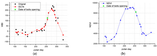
Figure 11. (a) The WBI time series, SG fit, and the midpoint extraction for bolls opening date. (b) The NDVI time series and the start date of bolls opening.

Figure 12 shows the start date of bolls opening at the four study sites, and the ratios of different bolls opening dates are compared with USDA phenological data. It is shown that the start date of bolls opening based on the WBI estimation and USDA are generally consistent in the U.S. The ground surveys and references showed that the start date of the bolls opening always occurred between 238 and 252 in the north of XJ, which is fitting for the estimation by WBI.

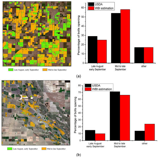
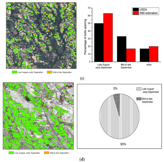
Figure 12. The bolls opening date of extraction based on WBI and compared with United States Department of Agriculture (USDA) statistic data. (a) MO-08, (b) CA-21, (c) GA-08, (d) XJ.

4. Discussion

A new white bolls index (WBI) is developed for automatic cotton mapping in this study, which enables effortless computation as well as mathematical simplicity. The proposed WBI can indicate the number of bolls opening, which turns larger with the increase of white bolls. Recently, more and more spectral indices for crop detection have been introduced based on remotely sensed time series, such as yellow flower indexes of canola and so on, showing the potential of spectral indexes in crop mapping. However, there are no reports for cotton mapping with spectral index, and the introduced WBI has shown an excellent effect for mapping cotton and accurate determination for cotton bolls opening date, which can be considered as an important contribution in this paper. It is worth noting that the WBI does not demand training data to map cotton fields.

In this paper, we used LDA on 10 bands of Sentinel-2 (B2: blue, B3: green, B4: red, B5: redEdge-1, B6: redEdge-2, B7: redEdge-3, B8: NIR, B8A: narrow NIR, B11: SWIR-1, B12: SWIR-2) to extract the WBI. To assess the importance of these different bands in WBI, we computed the correlation coefficients between WBI and WBI of removing a band. The lower the correlation coefficient, the more the band contributes. As Figure 13 shows, the blue, green, red, redEdge-3, and wide NIR bands show the higher weight in the construction of WBI, while the two SWIR bands are almost useless.

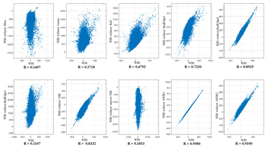
Figure 13. The correlation coefficient of WBI and WBI without a selected band.

The MSI sensor records the radiation from white bolls, green or yellow leaves and soil background. Provided that cotton bolls are white, it enhances the reflection of visible wavelengths, which leads to a higher and flatter reflectance of cotton in the blue, green, and red wavelengths as compared with the other crops. Therefore, blue, green, and red spectral bands give a higher contribution to the separation of cotton from other crops. Additionally, under the bolls opening stage, the growth of cotton is obviously weakened and nearly stopped. The leaves gradually declined and the photosynthesis decreased. While, red, redEdge-3, and narrow NIR can easily indicate the growth and health of vegetation, which can detect the senescence of vegetation and play important roles in WBI construction.

The new feature was mainly composed of visible and near IR bands. During the bolls opening stage, more and more white bolls are opening, which leads to the change of canopy reflectance. The color of white bolls can be expressed by visible bands, and the senescence of cotton can be indicated by near IR bands. As shown in Figure 14a, the ground reflectance of white bolls is shown as more “flat” in the visible bands, which indicates the color “white”. Meanwhile, the decreasing slope of RedEdge and the lower NIR show that the senescence of vegetation is beginning, marking the stage of bolls opening. Figure 14b displays the cotton’s harvested stage of the Xinjiang on 2014-10-16 from Google Earth, which shows the satellite view of the white bolls of the canopy.

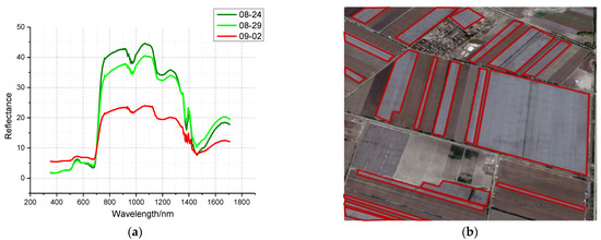
Figure 14. (a) The field spectral of cotton measured in Xinjiang. (b) The white bolls under satellite view in Xinjiang at 2014-10-16 from google earth.

The proposed index was developed for the bolls opening stage, lasting 15 to 30 days. The larger number of images without clouds in this period will lead to a better performance of WBI. Due to various climate and field management, the beginning date and rate of progress for bolls opening are diverse in different regions, as well as considering the obtained images with different temporal periods, all of which results in the subtle variation for thresholds. In our four study sites, we use 150, 170, 150, and 200 for MO-08, CA-21, GA-08, and XJ, respectively and achieve the best accuracy. According to our threshold test in study sites, the range [100–220] can be considered proper to detect white bolls within cropland.

It is worth noticing that the WBI describes the feature of white bolls for cotton, which is almost not affected by the various climates of regions. As Figure 12 shows, the survey shows that the four study sites have different dates for the bolls opening stage. However, the WBI only notices the feature of white bolls, which is a widespread trait of cotton in various regions and cannot be provided by other crops. Hence, based on WBI in the bolls opening period, the cotton can be easily mapped, and based on the WBI time series, SOS can be extracted by phenological methods as the beginning of bolls opening.

The SVM and 1DCNN need new training samples for new regions relative to the WBI classification; otherwise, they do not work satisfactorily. As shown in Table 4, SVM and 1DCNN can produce very high accuracy at the training site (MO-08) due to the test and training samples being from the same site, but they provide poorer performance in CA-21, GA-08, and XJ, which shows that machine learning models often dependent on training samples, and it is hard to extend to large-scale crop mapping due to the lack of training samples.

The results demonstrated that the proposed index shows the potential for automated cotton mapping without retraining at any location. The WBI is very effective for white bolls of UPLAND and PIMA cotton, of which white bolls are significant in the bolls opening stage, especially after defoliation, but the performance for tree cotton, the bolls of which are not present on the canopy, may not be very strong. The capability of WBI should be further assessed in future studies.

5. Conclusions

In the study, the white bolls index was developed based on the spectral characteristic during the bolls opening stage. White bolls, which are specific for cotton but cannot be seen by other crops, are derived as the white bolls index by linear discriminant analysis based on a Sentinel-2 time series. Rapid cotton mapping without training samples was performed by WBI, and the dates of bolls opening were identified by a WBI time series. The performance of the proposed index was assessed and compared with advanced classifiers such as SVM and 1DCNN, where WBI performed well without training samples. With the encouraging results of this study, the capability of WBI should be further assessed for cotton types with the lower significance of white bolls.

References

- Haider, A.; Bashir, A.; Husnain, M.I.U. Impact of agricultural land use and economic growth on nitrous oxide emissions: Evidence from developed and developing countries. Sci. Total Environ. 2020, 741, 140421. [Google Scholar] [CrossRef] [PubMed]
- Wardropper, C.B.; Mase, A.S.; Qiu, J.; Kohl, P.; Booth, E.G.; Rissman, A.R. Ecological worldview, agricultural or natural resource-based activities, and geography affect perceived importance of ecosystem services. Landsc. Urban Plan. 2020, 197, 103768. [Google Scholar] [CrossRef]
- Vermeulen, S.; Zougmoré, R.; Wollenberg, E.; Thornton, P.; Nelson, G.; Kristjanson, P.; Kinyangi, J.; Jarvis, A.; Hansen, J.; Challinor, A.; et al. Climate change, agriculture and food security: A global partnership to link research and action for low-income agricultural producers and consumers. Curr. Opin. Environ. Sustain. 2012, 4, 128–133. [Google Scholar] [CrossRef]
- Sun, S.; Li, C.; Chee, P.W.; Paterson, A.H.; Jiang, Y.; Xu, R.; Robertson, J.S.; Adhikari, J.; Shehzad, T. Three-dimensional photogrammetric mapping of cotton bolls in situ based on point cloud segmentation and clustering. ISPRS J. Photogramm. Remote Sens. 2020, 160, 195–207. [Google Scholar] [CrossRef]
- Jans, Y.; von Bloh, W.; Schaphoff, S.; Müller, C. Global cotton production under climate change—Implications for yield and water consumption. Hydrol. Earth Syst. Sci. Discuss. 2020, 2020, 1–27. [Google Scholar] [CrossRef]
- Khan, M.A.; Wahid, A.; Ahmad, M.; Tahir, M.T.; Ahmed, M.; Ahmad, S.; Hasanuzzaman, M. World Cotton Production and Consumption: An Overview. In Cotton Production and Uses: Agronomy, Crop Protection, and Postharvest Technologies; Ahmad, S., Hasanuzzaman, M., Eds.; Springer: Singapore, 2020; pp. 1–7. [Google Scholar] [CrossRef]
- Sawan, Z.M. Climatic variables: Evaporation, sunshine, relative humidity, soil and air temperature and its adverse effects on cotton production. Inf. Process. Agric. 2018, 5, 134–148. [Google Scholar] [CrossRef]
- Hao, P.Y.; Zhan, Y.L.; Wang, L.; Niu, Z.; Shakir, M. Feature Selection of Time Series MODIS Data for Early Crop Classification Using Random Forest: A Case Study in Kansas, USA. Remote Sens. 2015, 7, 5347–5369. [Google Scholar] [CrossRef]
- Xiong, J.; Thenkabail, P.S.; Gumma, M.K.; Teluguntla, P.; Poehnelt, J.; Congalton, R.G.; Yadav, K.; Thau, D. Automated cropland mapping of continental Africa using Google Earth Engine cloud computing. ISPRS J. Photogramm. Remote Sens. 2017, 126, 225–244. [Google Scholar] [CrossRef]
- Gupta, S.; Rajan, K.S. Extraction of training samples from time-series MODIS imagery and its utility for land cover classification. Int. J. Remote Sens. 2011, 32, 9397–9413. [Google Scholar] [CrossRef]
- Estel, S.; Kuemmerle, T.; Alcántara, C.; Levers, C.; Prishchepov, A.; Hostert, P. Mapping farmland abandonment and recultivation across Europe using MODIS NDVI time series. Remote Sens. Environ. 2015, 163, 312–325. [Google Scholar] [CrossRef]
- Peña, M.A.; Brenning, A. Assessing fruit-tree crop classification from Landsat-8 time series for the Maipo Valley, Chile. Remote Sens. Environ. 2015, 171, 234–244. [Google Scholar] [CrossRef]
- Cai, Y.; Guan, K.; Peng, J.; Wang, S.; Seifert, C.A.; Wardlow, B.; Li, Z. A high-performance and in-season classification system of field-level crop types using time-series Landsat data and a machine learning approach. Remote Sens. Environ. 2018, 210, 35–47. [Google Scholar] [CrossRef]
- Ouzemou, J.-E.; Harti, A.; Lhissou, R.; El Moujahid, A.; Bouch, N.; El Ouazzani, R.; Bachaoui, E.; Ghmari, A.E. Crop type mapping from pansharpened Landsat 8 NDVI data: A case of a highly fragmented and intensive agricultural system. Remote Sens. Appl. Soc. 2018, 11, 94–103. [Google Scholar] [CrossRef]
- Wardlow, B.D.; Egbert, S.L. Large-area crop mapping using time-series MODIS 250 m NDVI data: An assessment for the U.S. Central Great Plains. Remote Sens. Environ. 2008, 112, 1096–1116. [Google Scholar] [CrossRef]
- Zhai, Y.; Qu, Z.; Hao, L. Land Cover Classification Using Integrated Spectral, Temporal, and Spatial Features Derived from Remotely Sensed Images. Remote Sens. 2018, 10, 383. [Google Scholar] [CrossRef]
- Müller, H.; Rufin, P.; Griffiths, P.; Barros Siqueira, A.J.; Hostert, P. Mining dense Landsat time series for separating cropland and pasture in a heterogeneous Brazilian savanna landscape. Remote Sens. Environ. 2015, 156, 490–499. [Google Scholar] [CrossRef]
- Peña, M.A.; Liao, R.; Brenning, A. Using spectrotemporal indices to improve the fruit-tree crop classification accuracy. ISPRS J. Photogramm. Remote Sens. 2017, 128, 158–169. [Google Scholar] [CrossRef]
- Waldner, F.; Canto, G.S.; Defourny, P. Automated annual cropland mapping using knowledge-based temporal features. ISPRS J. Photogramm. Remote Sens. 2015, 110, 1–13. [Google Scholar] [CrossRef]
- Skakun, S.; Franch, B.; Vermote, E.; Roger, J.; Becker-Reshef, I.; Justice, C.; Kussul, N. Early season large-area winter crop mapping using MODIS NDVI data, growing degree days information and a Gaussian mixture model. Remote Sens. Environ. 2017, 195, 244–258. [Google Scholar] [CrossRef]
- Zhong, L.; Gong, P.; Biging, G.S. Efficient corn and soybean mapping with temporal extendability: A multi-year experiment using Landsat imagery. Remote Sens. Environ. 2014, 140, 1–13. [Google Scholar] [CrossRef]
- Shao, Y.; Lunetta, R.S.; Wheeler, B.; Iiames, J.S.; Campbell, J.B. An evaluation of time-series smoothing algorithms for land-cover classifications using MODIS-NDVI multi-temporal data. Remote Sens. Environ. 2016, 174, 258–265. [Google Scholar] [CrossRef]
- Massey, R.; Sankey, T.T.; Congalton, R.G.; Yadav, K.; Thenkabail, P.S.; Ozdogan, M.; Meador, A.J.S. MODIS phenology-derived, multi-year distribution of conterminous US crop types. Remote Sens. Environ. 2017, 198, 490–503. [Google Scholar] [CrossRef]
- Roy, D.P.; Yan, L. Robust Landsat-based crop time series modelling. Remote Sens. Environ. 2018, 238, 110810. [Google Scholar] [CrossRef]
- Zhong, L.; Hu, L.; Zhou, H. Deep learning based multi-temporal crop classification. Remote Sens. Environ. 2019, 221, 430–443. [Google Scholar] [CrossRef]
- Xu, J.; Zhu, Y.; Zhong, R.; Lin, Z.; Xu, J.; Jiang, H.; Huang, J.; Li, H.; Lin, T. DeepCropMapping: A multi-temporal deep learning approach with improved spatial generalizability for dynamic corn and soybean mapping. Remote Sens. Environ. 2020, 247, 111946. [Google Scholar] [CrossRef]
- Yan, Y.; Ryu, Y. Exploring Google Street View with deep learning for crop type mapping. ISPRS J. Photogramm. Remote Sens. 2021, 171, 278–296. [Google Scholar] [CrossRef]
- Zeng, L.; Wardlow, B.D.; Xiang, D.; Hu, S.; Li, D. A review of vegetation phenological metrics extraction using time-series, multispectral satellite data. Remote Sens. Environ. 2020, 237, 111511. [Google Scholar] [CrossRef]
- Ashourloo, D.; Shahrabi, H.S.; Azadbakht, M.; Aghighi, H.; Matkan, A.A.; Radiom, S. A Novel Automatic Method for Alfalfa Mapping Using Time Series of Landsat-8 OLI Data. IEEE J. Sel. Top. Appl. Earth Obs. Remote Sens. 2018, 11, 4478–4487. [Google Scholar] [CrossRef]
- Qiu, B.; Luo, Y.; Tang, Z.; Chen, C.; Lu, D.; Huang, H.; Chen, Y.; Chen, N.; Xu, W. Winter wheat mapping combining variations before and after estimated heading dates. ISPRS J. Photogramm. Remote Sens. 2017, 123, 35–46. [Google Scholar] [CrossRef]
- D’andrimont, R.; Taymans, M.; Lemoine, G.; Ceglar, A.; Yordanov, M.; van der Velde, M. Detecting flowering phenology in oil seed rape parcels with Sentinel-1 and -2 time series. Remote Sens Environ. 2020, 239, 111660. [Google Scholar] [CrossRef]
- Ashourloo, D.; Shahrabi, H.S.; Azadbakht, M.; Aghighi, H.; Nematollahi, H.; Alimohammadi, A.; Matkan, A.A. Automatic canola mapping using time series of sentinel 2 images. ISPRS J. Photogramm. Remote Sens. 2019, 156, 63–76. [Google Scholar] [CrossRef]
- United States Department of Agriculture, National Agriculture Statistics Service. Cotton Phenological Stages. Available online: https://www.nass.usda.gov/Publications/National_Crop_Progress/Terms_and_Definitions/index.php (accessed on 1 March 2021).
- Ali, H.; Afzal, M.N.; Ahmad, F.; Ahmad, S.; Atif, R. Effect of Sowing Dates, Plant Spacing and Nitrogen Application on Growth and Productivity on Cotton Crop. Int. J. Sci. Eng. Res. 2013, 2, 1–6. [Google Scholar]
- Wang, X. Impact and Adaptation of Climate Change on Cotton Phenology, Yield and Fiber Quality in Xinjiang. Ph.D. Thesis, China Agricultural University, Beijing, China, 2015. [Google Scholar]
- Zhao, L.U.; Li, L.I.; Tian, C.; Yan, X.; Wang, J.; Liu, Y. Calculation and analysis of cotton phenology in the Northern of Xinjiang. Arid Land Geogr. 2003, 26, 5. [Google Scholar]
- Belhumeur, P.N.; Hespanha, J.P.; Kriegman, D.J. Eigenfaces vs. Fisherfaces: Recognition Using Class Specific Linear Projection. IEEE Trans. Pattern Anal. Mach. Intell. 1997, 19, 711–720. [Google Scholar] [CrossRef]
- Bruzzone, L.; Chi, M.; Marconcini, M. A Novel Transductive SVM for Semisupervised Classification of Remote-Sensing Images. IEEE Trans. Geosci. Remote Sens. 2006, 44, 3363–3373. [Google Scholar] [CrossRef]
- Kranjčić, N.; Medak, D.; Župan, R.; Rezo, M. Support Vector Machine Accuracy Assessment for Extracting Green Urban Areas in Towns. Remote Sens. 2019, 11, 655. [Google Scholar] [CrossRef]
- Rustowicz, R.M. Crop Classification with Multi-Temporal Satellite Imagery; Stanford University: Stanford, CA, USA, 2019. [Google Scholar]
- Chen, J. A simple method for reconstructing a high-quality NDVI time-series data set based on the Savitzky–Golay filter. Remote Sens. Environ. 2004, 91, 332–344. [Google Scholar] [CrossRef]
- White, M.A.; Thornton, P.E.; Running, S.W. A continental phenology model for monitoring vegetation responses to interannual climatic variability. Glob. Biogeochem. Cycles 1997, 11, 217–234. [Google Scholar] [CrossRef]
Publisher’s Note: MDPI stays neutral with regard to jurisdictional claims in published maps and institutional affiliations. |
© 2021 by the authors. Licensee MDPI, Basel, Switzerland. This article is an open access article distributed under the terms and conditions of the Creative Commons Attribution (CC BY) license (https://creativecommons.org/licenses/by/4.0/).