Article

Mapping the Habitat Suitability of West Nile Virus Vectors in Southern Quebec and Eastern Ontario, Canada, with Species Distribution Modeling and Satellite Earth Observation Data

by
Yi Moua
1,2,*,
Serge Olivier Kotchi
1,2,
Antoinette Ludwig
1,2 and
Stéphanie Brazeau
1,2
1
Public Health Risk Sciences Division, National Microbiology Laboratory, Public Health Agency of Canada, 3200 rue Sicotte, Saint-Hyacinthe, QC J2S 2M2, Canada
2
Groupe de Recherche en Epidémiologie des Zoonoses et Santé Publique (GREZOSP), Faculty of Veterinary Medicine, University of Montréal, 3200 rue Sicotte, Saint-Hyacinthe, QC J2S 2M2, Canada
*
Author to whom correspondence should be addressed.
Remote Sens. 2021, 13(9), 1637; https://doi.org/10.3390/rs13091637
Submission received: 18 February 2021 / Revised: 5 April 2021 / Accepted: 17 April 2021 / Published: 22 April 2021
(This article belongs to the Section Ecological Remote Sensing)

Abstract

:
Transmission of vector-borne diseases (VBDs) relies on the presence of their vectors. Good knowledge of their habitat distribution could inform of their presence and then the potential transmission risk. In Canada, West Nile virus (WNV), a VBD transmitted by mosquitoes of the Culex genus to birds, humans, and other mammals, was first reported in 2002. Since then, human cases have been reported every year. To reduce the health burden of the disease and to guide the vector control efforts, this work aims to provide a map of habitat suitability of the main vectors of WNV, Culex pipiens-restuans, in southern Quebec and eastern Ontario at 30 m spatial resolution. Landsat 8-OTI/TIRS images were combined with existing geographical data to characterize vegetated and paved areas in urban and peri-urban areas and to create a land use land cover map related to environmental determinants of Culex pipiens-restuans. Landscape metrics were calculated to characterize the neighborhood environment. They were used with 1008 presence sites of the vectors to build species distribution models with Maxent, a model based on the maximum entropy principle, and to predict habitat suitability for Culex pipiens-restuans in the study area. The performance of the models was very good, with a mean area under the curve of 0.92 and a continuous Boyce index of 0.97. A habitat suitability map of the whole study area was created for Culex pipiens-restuans. The resulting map and environment analysis highlight the importance of the edge of vegetation and mixed or paved areas for the bio-ecology of Culex pipiens-restuans.

1. Introduction

Vector-borne diseases are a major public health concern. According to the World Health Organization, they cause more than 700,000 deaths annually [1]. Mosquitoes are considered one of the deadliest of all vectors [2]. They are responsible for transmitting malaria, chikungunya, zika, dengue, yellow fever, West Nile virus (WNV), Rift Valley fever virus, and others [2].
Culex genus are very important vectors of arboviroses such as WNV in North America. WNV human infection was first reported in North America in 1999, in New York City [3]. It has since spread across North America and reached Canada in 2002 [4]. In eastern Canada, Culex pipiens Linnaeus and Culex restuans Theobald are considered the main vectors of WNV. They are primarily ornithophilic but also feed on humans and other mammals [5,6]. The adults are usually identified as Culex pipiens-restuans (Cx. pipiens-restuans) complex because they are morphologically difficult to distinguish [7]. Spatial distribution of these vectors is defined by landscape characteristics that create suitable sites for breeding, feeding, and resting. Considered as urban mosquitoes [8,9], they have been found in vegetated areas, such as fragmented forest [10] and grass [11] situated in urban area. These vectors are capable of developing in artificial containers, such as used tires and bird baths, and in standing water such as detention and retention ponds and roadside ditches [12,13,14,15].
Following the Seventieth World Health Assembly held in 2017 in Geneva, the Global vector control response 2017–2030 [16] was developed. Its aim is to reduce the burden of vector-borne disease through key pillars of action that will enable a sustainable vector control locally adapted. Knowing the spatial distribution of vector habitat is crucial to helping public health authorities guide vector control and surveillance efforts. This information could be made available through use of species distribution models (SDM). These models relate species field observations (presence and absence data, when these latter are available) and environmental variables [17]—usually derived from remote sensing data—to produce a habitat suitability map of the species of interest. They were used successfully to predict and map the habitat of disease vectors such as Anopheles genus, vectors of malaria [18,19,20]; Aedes genus, vectors of dengue, chikungunya, zika, and yellow fever [21,22,23]; and Triatoma species, vectors of chagas disease [24,25].
In Canada, [26] produced a historical map of Cx. pipiens and Cx. restuans distribution, and [27] for Cx. pipiens at large spatial resolution. However, this knowledge should be updated and [28] highlighted the importance of characterizing the environment on a scale that is consistent with the vector bio-ecology. The purpose of this research, therefore, is to model the habitat suitability distribution of Cx. pipiens-restuans in southern Quebec and eastern Ontario using a fine spatial scale (30 m). Satellite remotely sensed data were used with species distribution modeling to achieve this goal.

2. Materials and Methods
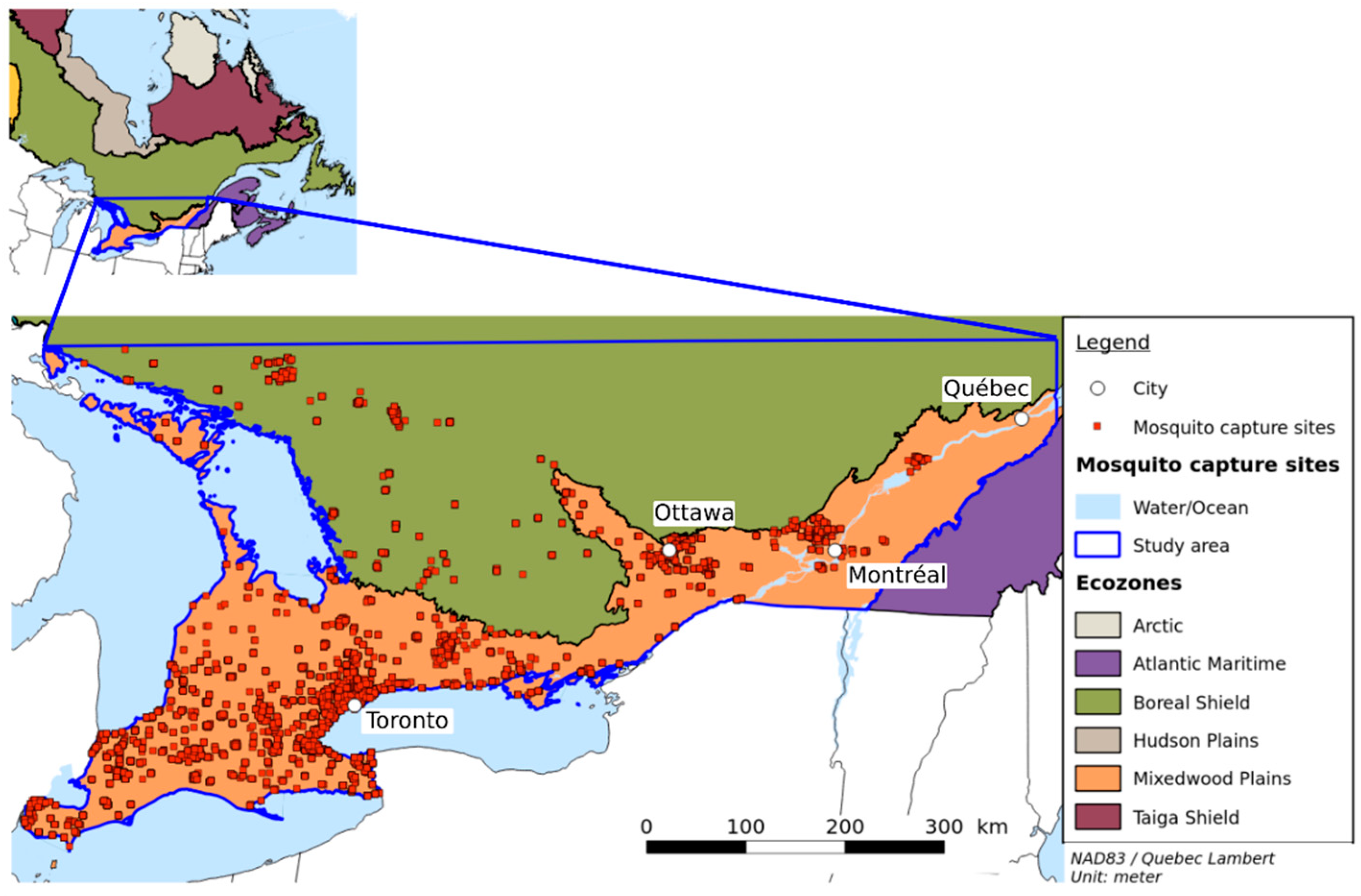
2.1. Study Area

The study area covers southern Quebec and eastern Ontario (see Figure 1), a surface area of 27,200,500 km2. Two major cities in this area are Montreal in the province of Quebec and Toronto in the province of Ontario. They are the two largest cities in Canada with respective populations of 1.7 million and 2.7 million people [29], followed by Ottawa, with 934,243 inhabitants and Québec with 531,902. All these cities are located in the Mixedwood Plains Ecozone [30], which is characterized by flat plains, a mean summer temperature of about 17 °C, a mean winter temperature of −5 °C, and annual precipitation of 720 mm to 1000 mm.

2.2. Maxent

Maxent is a machine learning method widely used in species distribution modeling to estimate the habitat suitability index (HSI) for species [31]. This model is based on the principle of maximum entropy, which consists in estimating an unknown probability distribution over the whole study area by finding the distribution that not only maximizes the entropy but also respects constraints imposed by environmental conditions at location where the species is present (see [31,32] for more details). Concretely, the estimated probability distribution assigns to each pixel of the whole study area a probability that is proportional to the probability of presence, interpreted as the HSI. As input, Maxent requires presence data, which is a set of geographical coordinates of the location where the given species was trapped or observed; a background, which is a set of sites reflecting environmental conditions available in the study area [33] and environmental features, which are a set of environmental variables that are relevant to the species.

2.3. Entomological Data

Mosquito capture data, seen in Figure 1 and Table 1, were provided by the Public Health Agency of Canada (PHAC) and Public Health Ontario (PHO). Captures were performed using Centers for Disease Control and Prevention light traps (CDC, [34]), Omni-Directional Fay-Prince Trap (OmniDirectional, [35]) and BG-Sentinel® traps (BGS, Biogents AG, Regensburg, Germany) between July and September. Mosquitoes were morphologically identified with taxonomic keys [36]. The dataset corresponds to 5239 different capture sites from 2002 to 2019, where 82 different species were identified, and only adult presence data was available. To ensure consistency between entomological and environmental data, only data between 2011 and 2019 were used in this study.

2.4. Environmental Data

2.4.1. Existing Geographical Data

To represent the known bio-ecology of Cx. pipiens-restuans or to create a proxy for it, several geographical data were chosen. There are the Annual crop inventory (ACI), a land use land cover map at national scale, provided yearly from 2011 to 2018 by Agriculture and Agri-Food Canada (AAFC); the National Hydro Network (NHN) from the Geobase Series provided by Natural Resources Canada (NRCan) that maps hydrographic features such as lakes, reservoirs, rivers, streams, canals, island, obstacles and construction; the Altitude data from the Canadian Digital Elevation Model (CDEM) provided by NRCan; the Wetlands layers from the Canadian Wetlands Inventory (CWI) of Unlimited Ducks Canada (UDC) and Ministère du Développement durable, de l’Environnement, de la Faune et des Parcs Québec and from Ontario Ministry of Natural Resources and Forestry and a Drainage layer, extracted from Soils of Canada, produced by AAFC, which provides the distribution of soil attributes such as drainage, texture of parent material, and kind of material at the national scale. They are summarized in Table A2 in Appendix B.

2.4.2. Land Use Land Cover

The current ACI layer, which is composed of 71 classes, was created in the context of agricultural inventory. Its urban class includes not only paved areas, but also residential areas (mix of vegetation and build-up areas), parks, water bodies, and wetlands. Cx. pipiens-restuans are known as urban mosquitoes that require vegetation to survive, then to obtain a Land use land cover (LULC) map related to these vectors, a classification of the urban areas (the term urban areas is used here for both urban and peri-urban areas) was made. To define the boundaries of urban areas, a buffer of 500 m around the Urban class of the ACI layer and the roads (from the National Roads Network (NRN) from NRCan) was created. We assumed that inhabited areas alongside rural roads were situated at 500 m from the roads. To cover the study area, 25 Landsat-8 OLI/TIRS scenes, with a cloud cover <20%, were selected from the months of July and August in the years from 2014 and 2018. Adjacent image scenes were combined to create a mosaic before the classification process. Based on the quality assessment provided with Landsat scenes, clouds, and cloud shadows were identified and removed for the index calculation. Indexes such as the normal difference vegetation index (NDVI), the normal difference built-up index (NDBI) and the normal difference water index (NDWI) were calculated. A supervised classification was performed on urban areas with a random forest classifier on calculated indices and the first three factorial axes of the Landsat spectral bands (one to seven). Four classes were defined: tree cover, which represents areas with a high cover of trees; grass vegetation/herbaceous, which is areas with grass cover; mixed area, which is a mix of vegetation and buildings and paved area.
Ground truth observations were randomly selected in the urban areas and were based on observations from Google Earth satellite images. The classification was performed with 75% of training data per class, randomly selected, and was tested with the remaining 25% (Table 2).
The resulting LULC (with an overall accuracy of 0.97 and a Kappa of 0.97, see the Appendix A) was aggregated with non-urban classes of the ACI layer and was completed by NHN and wetlands layers. All agriculture classes were aggregated to be Agriculture. Shrubland and Grassland were aggregated to be Shrubland class and all forest classes and tree cover in urban areas to be the class Forest. The final classes of the LULC map are listed in Table 3.

2.4.3. Geographical Derived Data

Refs. [9,10] highlighted the importance of the neighborhood landscape on Cx. pipiens-restuans populations. To describe and characterize the neighborhood, three kinds of landscape metrics were calculated for each pixel of the study area, the distance between each pixel of the study area and the nearest pixel of the given class; the percentage of the given class in a defined window and the diversity, representing the number of different classes in a defined window.
The defined window was 2 by 2 km, in order to reflect the mean flight distance of Cx. pipiens-restuans (1.37 km, [37]). In this window, the longest distance between the center and the edge is 1.4 km (2 × √2/2). Distance and percentage layers were produced for all of the LULC classes. Slope was derived from the DEM layer and the drainage layer was rasterized to a spatial resolution of 30 m. All raw and derived geographical data are summarized in Appendix B.
Data processing, classification and landscape analysis were done with free and open-source software, GRASS GIS [38] and R [39].

2.5. Model Calibration and Evaluation

In this study, to deal with collinearity, only variables with a Pearson correlation < |0.7| were chosen. Where there was high collinearity between two variables, the most ecologically relevant was retained. In total, 21 environmental variables were chosen (see Appendix B). Cx. pipiens-restuans presence data were considered biased because samples occurred mostly in anthropized areas. Ref. [33] highlighted that sampling bias can strongly impact the quality of the model. To correct the effect of the sampling bias, refs. [40,41] proposed filtering the presence sites based on their environmental characteristics, an environmental filtering. A factor analysis of mixed data [42] was performed on environmental data associated with the presence dataset. Next, a cluster analysis was performed, where the number of clusters is set to half of the number of presence sites [40]. One record was retained per cluster, i.e., a total of 1008 unique sites. Filtered presence sites, 10,000 randomly selected background sites, and 21 environmental variables were used as input for Maxent. Hinge and categorical features were selected for the environmental variables and the raw output was selected. In Maxent, the tuning of the regularization parameter permits to reduce overfitting [43]. It is by default set to 1. To select the optimal value, the R package ENMeval [44] was used. A set of values of regularization parameter varied from 1 to 5 with an increment of 0.5 were used to pre-built Maxent models, and a 5-fold cross-validation were used to calculate the Delta Akaike Information Criterion corrected (AICc, [45]), which is the difference between the AICc of a given model and the AICc of the model with the lowest AICc. The regularization value that permitted to have the lowest delta AICc was selected. The final model was fitted using 70% of the presence sites and tested using 30% and was computed using the version 3.4.1 of Maxent. A 10-fold cross-validation was also used to evaluate the prediction performance. The area under curves (AUC) and the continuous Boyce index (CBI, [46]) were calculated. According to [46], the CBI is better adapted to models that use presence-only data than AUC. Its value ranges between −1 and 1, a negative value means that the model is incorrect, a value close to zero means that the model is not different from a random model, and a positive value means that the predictions of the model are consistent with the presence distribution. The extrapolation option in Maxent was not used to avoid the model predicting in environments for which it was not trained. Finally, the contribution of each variable was estimated with a jackknife test and a HS map was produced.

3. Results

The test AUC was 0.92, the mean AUC from the 10-fold cross-validation was 0.92, and the CBI was 0.97. The HS map for Cx. pipiens-restuans is in Figure 2. The environmental variables that contributed the most to the models are the percentage of mixed area (MIX_PER), the percentage of paved area (PA_PER) and the distance to the nearest mixed area (MIX_DIST), with contributions of 53.5, 25.5, and 13.7% respectively. Other variables have a contribution lower than 5% (see Table 4).
The response curves of the environmental variables are represented in Figure 3. Among all LULC classes (Figure 3k), mixed area, paved area, and herbaceous are related to the highest habitat suitability index (HSI). For the drainage (Figure 3j), a soil poorly or imperfectly drained has a higher HSI than a soil moderately/well or rapidly drained. Figure 3a shows that the HSI increases to reach its highest value when the MIXED_PER is between 45 and 80%, after which the HSI decreases. The HSI is maximal when the MIX_DIST is at 0 and decreases rapidly with MIX_DIST (Figure 3b). The HSI is maximal for a PA_PER between 5 and 12%, after which it decreases (Figure 3c). The response curve of the percentage of herbaceous in 2 × 2 km (HERB_PER) follows the same pattern than the MIX_PER (Figure 3a,d). The HSI increases to reach its highest values when HERB_PER is at 15%, after which it decreases. For the percentage of forest in 2 × 2 km (FOR_PER, Figure 3e), the HSI is maximal when its value is between 3 and 20%, after which it decreases as the value increases. The HSI is maximal when the distance to the nearest forest (FOR_DIST) is close to 0, after which it decreases rapidly (Figure 3f), whereas the HSI increases to reach its maximal at a distance from the nearest shrubland (SHR_DIST) between 3000 m and 5900 m. The HSI increases rapidly for an altitude (ATL) between 10 and 180 m but decreases to reach 0 after an altitude higher than 500 m (Figure 3i). Figure 3h shows that as the distance to the nearest wetlands (WET_DIST) increases, the HSI increases.

4. Discussion

The purpose of this study was to map the distribution of Cx. pipiens-restuans at a fine scale in southern Quebec and eastern Ontario. We used Landsat images to characterize the presence of vegetation and paved areas in urban and peri-urban areas and combined with existing data to create a LULC map more adapted to Cx. pipiens-restuans. Landscape metrics layers were derived and used with the geographical coordinates of Cx. pipiens-restuans presence sites to build species distribution models using Maxent. These models have very good prediction performance, with a mean AUC of 0.92, a test AUC of 0.92, and a CBI of 0.97.
The resulting HS map (Figure 2) shows that a high HSI overlaps highly anthropized areas such as mixed areas, herbaceous, and paved areas. The mixed area class, which is a mix of vegetation and buildings, appears to contribute to the highest HSI (see Figure 3k). The herbaceous class represents grass or low vegetation in urban areas and near roads, which is generally adjacent to mixed areas. This is consistent with [8,47,48] that found that Cx. pipiens-restuans are highly associated with urbanized areas with vegetation. Figure 3k shows that forest and shrubland classes have a low HSI, and the response curve for FOR_PER (Figure 3e) shows that areas with a high proportion of forest are less suitable for Cx. pipiens-restuans than those with low proportions of forest. In fact, the HSI reaches its maximum at a FOR_PER between 3 and 20%, after which it decreases. Ref. [49] found that Cx. pipiens was present in forest canopy in their study area, which was a woodlot of 17 ha in Ontario. Given the window of 2 × 2 km used in our study, the surface area corresponding to 3% and 20% of forest is 6 and 40 ha, respectively, which is consistent with the surface area of the woodlot where [49] trapped Cx. pipiens. Our work highlights that only small percentage of forest contributes to a high HSI. An important observation on the HS map and in Figure 4a is that the interface between forest and mixed areas indicates a high HSI. This is linked to the feeding preference of Cx pipiens-restuans for birds, especially the American robin (Turdus migratorius) [5,50], that roosts mostly in trees in urban environments [51]. The study by [52] highlighted that, after the breeding period, American robins leave their nest, implying a diminution of the number of birds in urban areas. This diminution leads Cx. pipiens to feed on humans, implying a greater number of human WNV cases. These studies showed the importance of birds, their breeding sites, and human presence for these vectors. However, the paved areas, which are linked to human presence, are less suitable for Cx. pipiens-restuans than mixed areas. In Figure 4b, the larger the paved area is, the lower the HSI. Likewise, [11]’s study found that even though Cx. pipiens and Cx. restuans are urban mosquitoes, their numbers were very low in highly urbanized areas. While they could be present in paved areas, the lack of resting and feeding sites due to their ornithophilic nature, as mentioned above, make this environment somewhat less suitable than mixed areas.
Figure 3k and Figure 4c show that agricultural areas have a low HSI, unlike ref. [9], who found Cx. pipiens in agricultural land. This can be linked to the dataset used to build the models. Captures occurred in an agricultural area located in proximity to a mixed area, which explains how in Figure 4c the pixels corresponding to agriculture have a low HSI, while edges with mixed area have a higher HSI.
Wetlands have a very low HSI and the closer a pixel is to a wetland, the lower its HSI (Figure 3h,k), whereas [53] found Cx. pipiens-restuans in wetlands. However, it is important to note that in their study, they only mention larva presence, whereas in the present study, only adult data was available and very little sampling was done close to wetlands. Further captures should be made in this environment.
In Figure 3j, poorly or imperfectly drained soils have a higher HSI than moderately/well or rapidly drained soils, which is coherent with [9,54] who found that poorly and imperfectly drained can create temporary breeding sites for these vectors.
In this study, hydrological features are not suitable for Cx. pipiens-restuans and layers derived from the hydrological classes do not contribute to the model building. Although this is consistent with [55], who found a weak correlation between the proportion of open bodies of water surrounding their traps and Cx. pipiens populations, in our study no capture was made in or near water bodies, then the HSI in these areas should be taken with precaution. In the study by [9], they found a positive relationship between the distance to hydrographic features and Cx. pipiens-restuans populations, but they highlighted that is linked to the increased urban density in their study area. As these vectors can breed in artificial containers or temporary standing water [12,55,56], and because they prefer artificial habitats [13], their presence is related to breeding sites that humans create.
In [26,27] the HS of Cx. pipiens was observed or estimated with climatic variables across Canada. On their maps, the HSI is high on all the current study area, whereas north is mostly composed of forest and hydrological features (see in Figure A1 of Appendix A), a less favorable habitat for Cx. pipiens-restuans. These differences may be explained by the difference in spatial scale used in the three studies ([26,27] and this current study) and the fact that, with a finer spatial scale, as the one used here, it is possible to capture local variation of habitat suitability which is more adapted to target locally vector control activities.

5. Conclusions

This study permits to have a habitat suitability map for Culex pipiens-restuans in southern Quebec and eastern Ontario. It highlights the importance of characterizing the environment not only by using land use and land cover map but also derived layers associated with proximity (distance to a class) or zonal statistics (percentage of the class in a given window) variables. The paper shows the importance of vegetation presence in urban areas for Cx. pipiens-restuans. Finally, this study permits to complete the current knowledge of the spatial distribution of Cx. pipiens-restuans and the habitat suitability map can be used by Quebec and Ontario provinces to target future vector control activities.

Author Contributions

Y.M. participated in the research design, data processing, program development, analysis and interpretation of the results, and prepared the manuscript. S.O.K., A.L. and S.B. participated in the research design and reviewed the manuscript. All authors have read and agreed to the published version of the manuscript.

Funding

This study is funded by Canadian Space Agency under the Climate Change Impacts and Ecosystem Resilience (CCIER) program.

Informed Consent Statement

Not applicable.

Data Availability Statement

The data used for this study was obtained from Public Health Ontario and Public Health Agency of Canada under license for the current study and are not publicly available.

Acknowledgments

We thank Public Health Ontario, Université de Montréal, Groupe de Recherche en Épidéniologie des Zoonoses et Santé Publique (GREZOSP), GDG Environment and Public Health Agency of Canada for providing mosquito surveillance data.

Conflicts of Interest

The authors declare no conflict of interest.

Appendix A

Table A1. Confusion matrix of the land use land cover classification.
References
ClassesPavedTree CoverGrass CoverMixed AreaUser Accuracy
Paved43209197.73%
Tree cover05503498.74%
Grass cover51132492.95%
Mixed area02651198.46%
Producer accuracy98.85%99.46%98.27%88%
Overall accuracy = 97.89%; Kappa = 97.04%.
Figure A1. Resulted Land use land cover map.
Remotesensing 13 01637 g0a1

Appendix B

Table A2. Environmental data. Derived layers with an asterisk were not used to build the models.
Geographical LayersProvidersDateInitial Spatial ResolutionClasses or Value RangesDerived LayersFinal Spatial Resolution
Annual crop inventory (ACI)AAFC 1201630 mIn total 71 different classes were defined: four forest classes, 60 agriculture classes, and seven other classes (urban, shrubland, grassland, wetlands, bare soil, water and cloud)
-
Land use land cover (LULC)
-
Distance to the nearest forest (FOR_DIST)
-
Percentage of forest in 2 × 2 km (FOR_PER)
-
Distance to the nearest mixed area (MIX_DIST)
-
Percentage of mixed area in 2 × 2 km (MIX_PER)
-
Distance to the nearest paved area (PA_DIST)*
-
Percentage of paved area in 2 × 2 km (PA_PER)
-
Distance to the nearest bare soil (BARE_DIST)
-
Percentage of bare soil in 2 × 2 km (BARE_PER)
-
Distance to the nearest herbaceous (HER_DIST) *
-
Percentage of herbaceous in 2 × 2 km (HER_PER)
-
Distance to the nearest shrubland (SHR_DIST)
-
Percentage of shrubland in 2 × 2 km (SHR_PER)
-
Distance to the nearest wetlands (WET_DIST)
-
Percentage of wetlands in 2 × 2 km (WET_PER)
-
Distance to the nearest agriculture (AGRI_DIST)
-
Percentage of agriculture in 2 × 2 km (AGRI_PER)
-
Distance to the nearest hydrological features (HYD_DIST)
-
Percentage of hydrological features in 2 × 2 km (HYD_PER)
-
Classes diversity (DIV)
-
NDVI *
-
NDBI *
-
NDWI *
30 m
National Hydro Network (NHN)NRCan 220041:50,000-
National Roads Network (NRN)NRCan20071:10,000-
WetlandsOntario Ministry of Natural Resources and Forestry 2011–Present1:10,000Wetlands are classified into six classes: bog, fen, marsh, swamp, open water and unknown
Unlimited Ducks Canada and Ministère du Développement durable, de l’Environnement, de la Faune et des Parcs Québec2009–Present1:20,000Wetlands are classified into seven classes: marsh, swamp, peatland fen, peatland bog, peatland bog, peatland forested, shallow water and wet meadow.
Landsat-8 OLIUnited States Geological Survey2014–201730 m-
Canadian Digital Elevation Model (CDEM)NRCan1945–201120 m0–1128 m
-
Altitude (ALT)
-
Slope (SLO)
30 m
Soils of Canada, DerivedNRCanOriginally produced in 19801:5,000,000The drainage is classified into five classes: Unclassified, Poorly drained, Imperfectly drained, Moderately/Well drained and Rapidly drainedDrainage (DRA)30 m
1 AAFC: Agriculture and Agri-food of Canada; 2 NRCan: Natural Resources of CanadaReferences.

References

  1. World Health Organization. Vector-Borne Diseases. Available online: https://www.who.int/news-room/fact-sheets/detail/vector-borne-diseases (accessed on 21 September 2020).
  2. World Health Organization. Mosquito-Borne Diseases. Available online: http://www.who.int/neglected_diseases/vector_ecology/mosquito-borne-diseases/en/ (accessed on 21 September 2020).
  3. Nash, D.; Mostashari, F.; Fine, A.; Miller, J.; O’Leary, D.; Murray, K.; Huang, A.; Rosenberg, A.; Greenberg, A.; Sherman, M.; et al. The Outbreak of West Nile Virus Infection in the New York City Area in 1999. Engl. J. Med. 2001, 344, 1807–1814. [Google Scholar] [CrossRef] [PubMed] [Green Version]
  4. Pepperell, C.; Rau, N.; Krajden, S.; Kern, R.; Humar, A.; Mederski, B.; Simor, A.; Low, N.E.; McGeer, A.; Mazzulli, T.; et al. West Nile virus infection in 2002: Morbidity and mortality among patients admitted to hospital in southcentral Ontario. Can. Med. Assoc. J. 2003, 168, 1399–1405. [Google Scholar]
  5. Hamer, G.L.; Kitron, U.D.; Brawn, J.D.; Loss, S.R.; Ruiz, M.O.; Goldberg, T.L.; Walker, E.D. Culex pipiens(Diptera: Culicidae): A Bridge Vector of West Nile Virus to Humans. J. Med. Èntomol. 2008, 45, 125–128. [Google Scholar] [CrossRef] [Green Version]
  6. Apperson, C.S.; Hassan, H.K.; Harrison, B.A.; Savage, H.M.; Aspen, S.E.; Farajollahi, A.; Crans, W.; Daniels, T.J.; Falco, R.C.; Benedict, M.; et al. Host Feeding Patterns of Established and Potential Mosquito Vectors of West Nile Virus in the Eastern United States. Vector-Borne Zoonotic Dis. 2004, 4, 71–82. [Google Scholar] [CrossRef] [PubMed]
  7. Kilpatrick, A.M.; Kramer, L.D.; Campbell, S.R.; Alleyne, E.O.; Dobson, A.P.; Daszak, P. West Nile Virus Risk Assessment and the Bridge Vector Paradigm. Emerg. Infect. Dis. 2005, 11, 425–429. [Google Scholar] [CrossRef] [PubMed]
  8. Diuk-Wasser, M.A.; Brown, H.E.; Andreadis, T.G.; Fish, D. Modeling the Spatial Distribution of Mosquito Vectors for West Nile Virus in Connecticut, USA. Vector-Borne Zoonotic Dis. 2006, 6, 283–295. [Google Scholar] [CrossRef] [PubMed] [Green Version]
  9. Trawinski, P.R.; Mackay, D.S. Identification of Environmental Covariates of West Nile Virus Vector Mosquito Population Abundance. Vector-Borne Zoonotic Dis. 2010, 10, 515–526. [Google Scholar] [CrossRef] [PubMed]
  10. Gardner, A.M.; Lampman, R.L.; Muturi, E.J. Land Use Patterns and the Risk of West Nile Virus Transmission in Central Illinois. Vector-Borne Zoonotic Dis. 2014, 14, 338–345. [Google Scholar] [CrossRef] [Green Version]
  11. Brown, H.; Diuk-Wasser, M.; Andreadis, T.; Fish, D. Remotely-Sensed Vegetation Indices Identify Mosquito Clusters of West Nile Virus Vectors in an Urban Landscape in the Northeastern United States. Vector-Borne Zoonotic Dis. 2008, 8, 197–206. [Google Scholar] [CrossRef] [PubMed] [Green Version]
  12. Wood, D.M.; Dang, P.T.; Ellis, R.A. The Mosquitoes of Canada: Diptera, Culicidae; The Insects and Arachnids of Canada; Agriculture Canada; Canadian Govt. Pub. Centre, Supply and Services Canada: Hull, QC, Canada, 1979; ISBN 978-0-660-10402-7. [Google Scholar]
  13. Jackson, M.J.; Gow, J.L.; Evelyn, M.J.; Meikleham, N.E.; McMahon, T.S.; Koga, E.; Howay, T.J.; Wang, L.; Yan, E. Culex Mosquitoes, West Nile Virus, and the Application of Innovative Management in the Design and Management of Stormwater Retention Ponds in Canada. Water Qual. Res. J. 2009, 44, 103–110. [Google Scholar] [CrossRef]
  14. Mackay, A.J.; Muturi, E.J.; Ward, M.P.; Allan, B.F. Cascade of ecological consequences for West Nile virus transmission when aquatic macrophytes invade stormwater habitats. Ecol. Appl. 2016, 26, 219–232. [Google Scholar] [CrossRef]
  15. Deichmeister, J.M.; Telang, A. Abundance of West Nile virus mosquito vectors in relation to climate and landscape variables. J. Vector Ecol. 2011, 36, 75–85. [Google Scholar] [CrossRef] [PubMed]
  16. World Health Organization. Global Vector Control Response 2017–2030; World Health Organization: Geneva, Switzerland, 2017. [Google Scholar]
  17. Guisan, A.; Thuiller, W. Predicting species distribution: Offering more than simple habitat models. Ecol. Lett. 2005, 8, 993–1009. [Google Scholar] [CrossRef]
  18. Alimi, T.O.; Fuller, D.O.; Qualls, W.A.; Herrera, S.V.; Arevalo-Herrera, M.; Quinones, M.L.; Lacerda, M.V.G.; Beier, J.C. Predicting potential ranges of primary malaria vectors and malaria in northern South America based on projected changes in climate, land cover and human population. Parasites Vectors 2015, 8, 1–16. [Google Scholar] [CrossRef] [PubMed] [Green Version]
  19. Zeilhofer, P.; Dos Santos, E.S.; Ribeiro, A.L.; Miyazaki, R.D.; Dos Santos, M.A. Habitat suitability mapping of Anopheles darlingi in the surroundings of the Manso hydropower plant reservoir, Mato Grosso, Central Brazil. Int. J. Health Geogr. 2007, 6, 7. [Google Scholar] [CrossRef] [PubMed] [Green Version]
  20. Moua, Y.; Roux, E.; Girod, R.; Dusfour, I.; De Thoisy, B.; Seyler, F.; Briolant, S. Distribution of the Habitat Suitability of the Main Malaria Vector in French Guiana Using Maximum Entropy Modeling. J. Med. Èntomol. 2016, 54, 606–621. [Google Scholar] [CrossRef] [PubMed]
  21. Cardoso-Leite, R.; Vilarinho, A.C.; Novaes, M.C.; Tonetto, A.F.; Vilardi, G.C.; Guillermo-Ferreira, R. Recent and future environmental suitability to dengue fever in Brazil using species distribution model. Trans. R. Soc. Trop. Med. Hyg. 2014, 108, 99–104. [Google Scholar] [CrossRef] [PubMed]
  22. Fatima, S.H.; Atif, S.; Rasheed, S.B.; Zaidi, F.; Hussain, E. Species Distribution Modelling ofAedes aegyptiin two dengue-endemic regions of Pakistan. Trop. Med. Int. Health 2016, 21, 427–436. [Google Scholar] [CrossRef] [PubMed] [Green Version]
  23. Santos, J.; Meneses, B.M. An integrated approach for the assessment of the Aedes aegypti and Aedes albopictus global spatial distribution, and determination of the zones susceptible to the development of Zika virus. Acta Trop. 2017, 168, 80–90. [Google Scholar] [CrossRef] [PubMed]
  24. Peterson, A.T.; Sánchez-Cordero, V.; Beard, C.B.; Ramsey, J.M. Ecologic niche modeling and potential reservoirs for Chagas disease, Mexico. Emerg. Infect. Dis. 2002, 8, 662–667. [Google Scholar] [CrossRef] [PubMed]
  25. Sarkar, S.; Strutz, S.E.; Frank, D.M.; Rivaldi, C.; Sissel, B.; Sánchez–Cordero, V. Chagas Disease Risk in Texas. PLoS Negl. Trop. Dis. 2010, 4, e836. [Google Scholar] [CrossRef]
  26. Darsie, R.F.; Ward, R.A.; Chang, C.C.; Litwak, T. Identification and Geographical Distribution of the Mosquitoes of North America, North of Mexico; University Press of Florida: Gainesville, FL, USA, 1983; ISBN 978-0-8130-6233-4. [Google Scholar]
  27. Hongoh, V.; Hoen, A.G.; Aenishaenslin, C.; Waaub, J.-P.; Bélanger, D.; Michel, P. The Lyme-MCDA Consortium Spatially explicit multi-criteria decision analysis for managing vector-borne diseases. Int. J. Health Geogr. 2011, 10, 70. [Google Scholar] [CrossRef] [Green Version]
  28. Kotchi, S.O.; Brazeau, S.; Ludwing, A.; Aube, G.; Berthiaume, P. Earth Observation and Indicators Pertaining to Determinants of Health—An Approach to Support Local Scale Characterization of Environmental Determinants of Vector-Borne Diseases. In Proceedings of the ESA Communications, ESTEC, Noordwijk, The Netherlands, 9 May 2016; Volume 740, p. 9. [Google Scholar]
  29. Statistics Canada Census in Brief: Municipalities in Canada with the Largest and Fastest-Growing Populations between 2011 and 2016. Available online: https://www12.statcan.gc.ca/census-recensement/2016/as-sa/98-200-x/2016001/98-200-x2016001-eng.cfm (accessed on 28 October 2020).
  30. ESTR Secretariat Mixedwood. Plains ecozone + evidence for key finding summary. In Biodiversity: Ecosystem Status and Trends 2010; Evidence for Key Findings Summary Report No7; Canadian Councils of Resource Ministers: Ottawa, ON, Canada, 2016; ISBN 978-1-100-25867-6. [Google Scholar]
  31. Phillips, S.J.; Anderson, R.P.; Schapire, R.E. Maximum entropy modeling of species geographic distributions. Ecol. Model. 2006, 190, 231–259. [Google Scholar] [CrossRef] [Green Version]
  32. Elith, J.; Phillips, S.J.; Hastie, T.; Dudík, M.; Chee, Y.E.; Yates, C.J. A statistical explanation of MaxEnt for ecologists. Divers. Distrib. 2010, 17, 43–57. [Google Scholar] [CrossRef]
  33. Phillips, S.J.; Dudík, M.; Elith, J.; Graham, C.H.; Lehmann, A.; Leathwick, J.; Ferrier, S. Sample selection bias and presence-only distribution models: Implications for background and pseudo-absence data. Ecol. Appl. 2009, 19, 181–197. [Google Scholar] [CrossRef] [PubMed] [Green Version]
  34. Sudia, W.D.; Chamberlain, R.W. Battery-operated light trap, an improved model. By W. D. Sudia and R. W. Chamberlain, 1962. J. Am. Mosq. Control. Assoc. 1988, 4, 126–129. [Google Scholar]
  35. Fay, R.W.; Prince, W.H. A Modified Visual Trap for Aedes Aegypti. Mosq. News 1970, 30, 20–23. [Google Scholar]
  36. Wood, D.M. Clés des Genres et des Espèces de Moustiques du Canada: Diptera:Culicidae; Agriculture Canada: Ottawa, ON, Canada, 1983; ISBN 978-0-660-91096-3. [Google Scholar]
  37. Ciota, A.T.; Drummond, C.L.; Ruby, M.A.; Drobnack, J.; Ebel, G.D.; Kramer, L.D. Dispersal of Culex mosquitoes (Diptera: Culicidae) from a wastewater treatment facility. J. Med. Èntomol. 2012, 49, 35–42. [Google Scholar] [CrossRef] [PubMed] [Green Version]
  38. GRASS Development Team. Geographic Resources Analysis Support System (GRASS) Software, Version 7.2. Available online: https://grass.osgeo.org/ (accessed on 21 September 2020).
  39. R Core Team. A Language and Environment for Statistical Computing; R Foundation for Statistical Computing: Vienna, Austria, 2016. [Google Scholar]
  40. Fourcade, Y.; Engler, J.O.; Rödder, D.; Secondi, J. Mapping Species Distributions with MAXENT Using a Geographically Biased Sample of Presence Data: A Performance Assessment of Methods for Correcting Sampling Bias. PLoS ONE 2014, 9, e97122. [Google Scholar] [CrossRef] [Green Version]
  41. Varela, S.; Anderson, R.P.; García-Valdés, R.; Fernández-González, F. Environmental filters reduce the effects of sampling bias and improve predictions of ecological niche models. Ecography 2014, 37, 1084–1091. [Google Scholar] [CrossRef]
  42. Pagès, J. Analyse Factorielle de Données Mixtes. Rev. Stat. Appl. 2004, 52, 93–111. [Google Scholar]
  43. Merow, C.; Smith, M.J.; Silander, J.A. A practical guide to MaxEnt for modeling species’ distributions: What it does, and why inputs and settings matter. Ecography 2013, 36, 1058–1069. [Google Scholar] [CrossRef]
  44. Muscarella, R.; Galante, P.J.; Soley-Guardia, M.; Boria, R.A.; Kass, J.M.; Uriarte, M.; Anderson, R.P. ENMeval: An R package for conducting spatially independent evaluations and estimating optimal model complexity forMaxentecological niche models. Methods Ecol. Evol. 2014, 5, 1198–1205. [Google Scholar] [CrossRef]
  45. Warren, D.L.; Seifert, S.N. Ecological niche modeling in Maxent: The importance of model complexity and the performance of model selection criteria. Ecol. Appl. 2011, 21, 335–342. [Google Scholar] [CrossRef] [PubMed] [Green Version]
  46. Hirzel, A.H.; Le Lay, G.; Helfer, V.; Randin, C.; Guisan, A. Evaluating the ability of habitat suitability models to predict species presences. Ecol. Model. 2006, 199, 142–152. [Google Scholar] [CrossRef]
  47. Myer, M.H.; Campbell, S.R.; Johnston, J.M. Spatiotemporal modeling of ecological and sociological predictors of West Nile virus in Suffolk County, NY, mosquitoes. Ecosphere 2017, 8, e01854. [Google Scholar] [CrossRef] [PubMed] [Green Version]
  48. Andreadis, T.G. The Contribution of Culex pipiens Complex Mosquitoes to Transmission and Persistence of West Nile Virus in North America. J. Am. Mosq. Control Assoc. 2012, 28, 137–151. [Google Scholar] [CrossRef] [PubMed]
  49. Russell, C.; Hunter, F.F. Influence of elevation and avian or mammalian hosts on attraction of Culex pipiens (Diptera: Culicidae) in southern Ontario. Can. Èntomol. 2010, 142, 250–255. [Google Scholar] [CrossRef]
  50. Taieb, L.; Ludwig, A.; Ogden, N.H.; Lindsay, R.L.; Iranpour, M.; Gagnon, C.A.; Bicout, D.J. Bird Species Involved in West Nile Virus Epidemiological Cycle in Southern Québec. Int. J. Res. Public Health 2020, 17, 4517. [Google Scholar] [CrossRef] [PubMed]
  51. Harris, M.L.; Wilson, L.K.; Elliott, J.E.; Bishop, C.A.; Tomlin, A.D.; Henning, K.V. Transfer of DDT and metabolites from fruit orchard soils to American robins (Turdus migratorius) twenty years after agricultural use of DDT in Canada. Arch. Contam. Toxicol. 2000, 39, 205–220. [Google Scholar] [CrossRef] [PubMed]
  52. Kilpatrick, A.M.; Kramer, L.D.; Jones, M.J.; Marra, P.P.; Daszak, P. West Nile Virus Epidemics in North America Are Driven by Shifts in Mosquito Feeding Behavior. PLoS Biol. 2006, 4, e82. [Google Scholar] [CrossRef] [PubMed]
  53. Irwin, P.; Arcari, C.; Hausbeck, J.; Paskewitz, S. Urban Wet Environment as Mosquito Habitat in the Upper Midwest. EcoHealth 2008, 5, 49–57. [Google Scholar] [CrossRef] [PubMed]
  54. Doran, B.R.; Lewis, D.J. The species composition and seasonal distribution of mosquitoes in vernal pools in suburban Montreal, Quebec. J. Am. Mosq. Control Assoc. 2003, 19, 339–346. [Google Scholar]
  55. Yoo, E.-H.; Chen, D.; Diao, C.; Russell, C. The Effects of Weather and Environmental Factors on West Nile Virus Mosquito Abundance in Greater Toronto Area. Earth Interact. 2016, 20, 1–22. [Google Scholar] [CrossRef]
  56. Yee, N.A. Tires as Habitats for Mosquitoes: A Review of Studies within the Eastern United States: Table 1. J. Med. Èntomol. 2008, 45, 581–593. [Google Scholar] [CrossRef] [PubMed]
Figure 1. The study area and mosquito capture sites. The study area is situated mainly in the Mixedwood Plains and the southern part of the Boreal shield.
Remotesensing 13 01637 g001
Figure 2. Habitat suitability map for Cx. pipiens-restuans.
Remotesensing 13 01637 g002
Figure 3. Response curves of environmental variables (only variables with a percentage of contribution to the model higher than zero are presented, see Table 4), (a) Percentage of mixed area, (b) Distance to mixed area, (c) Percentage of paved area, (d) Percentage of herbaceous, (e) Percentage of forest, (f) Distance to forest, (g) Distance to shrubland, (h) Distance to wetlands, (i) Altitude, (j) Drainage classes and (k) LULC classes. For categorical variables, the bars represent the mean habitat suitability index (HSI), and the error bars represent the standard deviation. For continuous variables, the curves represent the mean HSI and the grey shading represents the interval between the maximum and minimum. In (k) water represents hydrological features.
Remotesensing 13 01637 g003
Figure 4. Blown-up views of the HS map showing the interface between (a) mixed area and forest, (b) mixed area and paved area, and (c) mixed area and agriculture.
Remotesensing 13 01637 g004
Table 1. Mosquito capture data.
ProvidersDatesNumber of Capture Sites/Number of Capture Sites Where Cx. pipiens-restuans Were PresentTraps
PHAC 12006–2016120/111CDC 2
PHAC2014–201624/24CDC
PHAC2017–201894/91CDC
PHO 12012–20195001/4406CDC, OmniDirectional 2, BGS 2
1 PHAC: Public Health Agency of Canada; PHO: Public Health Ontario; 2 CDC: Centers for Disease Control and Prevention light traps; OmniDirectional: Omni-Directional Fay-Prince trap; BGS: BG-Sentinel®.
Table 2. Size of training and test sets for each class.
ClassesTrain (75%)Test (25%)
Forest/tree cover1289553
Grass vegetation/herbaceous1214520
Mixed351150
Paved1020437
Table 3. Final classes of the land use land cover map.
ClassesAbbreviationsDescription
AgricultureAGAnnual crops, pastures
WaterWARivers, lakes, reservoirs
WetlandsWEBogs, fens, marshes, swamps, shallow water
ShrublandSHGrassland and shrubland
ForestFOConiferous, broadleaf, mixed wood
In urban areas: may be parks with a high cover of trees
HerbaceousHBUrban and peri-urban areas with grass cover, such as park without tree, golf courses, garden
Mixed areaMAMix of building and vegetation, such as residential areas with gardens, industrial sites with vegetation
Paved areaPABuilt-up lands with paved surface without vegetation
Bare soilBSBare soil
CloudCLCloud
Table 4. Percentage of contribution of each environmental variable. Only variables with a percentage of contribution higher than zero are represented.
Environmental VariablesPercentage of Contribution
MIX_PER53.5
PA_PER25.5
MIX_DIST13.7
LULC2.2
DRA1.3
SHR_DIST1.2
HERB_PER0.9
FOR_DIST0.9
ALT0.5
FOR_PER0.2
WET_DIST0.2
Note: MIX_PER: percentage of mixed area in 2 × 2 km; PA_PER: Percentage of paved area in 2 × 2 km; MIX_DIST: distance to the nearest mixed area; HER_PER: percentage of herbaceous area in 2 × 2 km; LULC: Land use land cover; FOR_DIST: Distance to the nearest forest; SHR_DIST: distance to the nearest shrubland; DRA: drainage; ALT: Altitude; FOR_PER: Percentage of forest in 2 × 2 km; AGRI_PER: Percentage of agriculture in 2 × 2 km; WET_DIST: distance to the nearest wetlands.
Publisher’s Note: MDPI stays neutral with regard to jurisdictional claims in published maps and institutional affiliations.

