Abstract
UAV-based multispectral multi-camera systems are widely used in scientific research for non-destructive crop traits estimation to optimize agricultural management decisions. These systems typically provide data from the visible and near-infrared (VNIR) domain. However, several key absorption features related to biomass and nitrogen (N) are located in the short-wave infrared (SWIR) domain. Therefore, this study investigates a novel multi-camera system prototype that addresses this spectral gap with a sensitivity from 600 to 1700 nm by implementing dedicated bandpass filter combinations to derive application-specific vegetation indices (VIs). In this study, two VIs, GnyLi and NRI, were applied using data obtained on a single observation date at a winter wheat field experiment located in Germany. Ground truth data were destructively sampled for the entire growing season. Likewise, crop heights were derived from UAV-based RGB image data using an improved approach developed within this study. Based on these variables, regression models were derived to estimate fresh and dry biomass, crop moisture, N concentration, and N uptake. The relationships between the NIR/SWIR-based VIs and the estimated crop traits were successfully evaluated (R2: 0.57 to 0.66). Both VIs were further validated against the sampled ground truth data (R2: 0.75 to 0.84). These results indicate the imaging system’s potential for monitoring crop traits in agricultural applications, but further multitemporal validations are needed.
1. Introduction
In light of the increase in the global population, food security will be a significant concern in the next decades [1]. This security can be enhanced by good decision support in crop management, and for that purpose, non-destructive imaging technologies are of key importance, especially when it comes to diagnosing in-season site-specific crop status [2,3,4]. In this context, the most promising research area is precision agriculture that utilizes proximal and remote sensing technologies [5]. In the last decade, remote sensing of crops changed significantly in two ways: (i) open access satellite data enabled the analysis of large multi-temporal data sets in spatial resolutions of at least 10 to 20 m [6,7] and (ii) progress in new data acquisition and analysis approaches were facilitated by the fast development of Unmanned Aerial Vehicles (UAVs) as sensor carrying platforms for RGB, multi- and hyperspectral, LiDAR, or thermal sensing systems [8,9,10,11,12]. Studies on UAV-based sensing of crops have demonstrated the potential of such non-destructive approaches in determining crop traits [13,14,15]. As shown in many studies since 2013, robust crop height data, which have a strong link to biomass, can be derived from stereo-photogrammetric and GIS analyses [16,17,18].
A general problem is that estimation of nitrogen concentration (NC) from spectral data over different plant constituents is only indirectly possible since NC has no unique spectral features in the VNIR-SWIR range. According to Berger et al. [19], most studies only use the VNIR (400 to 1000 nm) to determine crop traits, especially nitrogen, in relation to chlorophyll. However, this approach neglects the foliar biochemical contents, such as plant proteins, which have faint spectral components in the short-wave infrared (SWIR) and whose link to different crop traits has hardly been studied so far, leading Berger et al. [19] to recommend including this domain explicitly. Likewise, Stroppiana et al. [20] state that this wavelength range has the potential to reveal new approaches or indices for vegetation monitoring. Herrmann et al. [21] attribute the under-exploration of this domain to traditional and to technical aspects. Those aspects have meant that expensive and heavyweight equipment, such as portable field-spectroradiometers or hyperspectral scanner systems on various airborne platforms, have been used so far. As a result of technological advances in recent years, however, these former shortcomings are increasingly being overcome, enabling new application scenarios. Exemplary in this context, Kandylakis et al. [22] developed a methodology for estimating water stress in vineyards using the unfiltered spectral response (900 to 1700 nm) of a SWIR imager combined with a VNIR multispectral multi-camera system (Parrot Sequoia; Parrot Drone SAS, Paris, France) using a UAV. However, no multi-camera system based on VIS-enhanced InGaAs (600 to 1700 nm) cameras with application-specific applicable narrow-band bandpass filters appear to have been used.
Within the latest research activities on UAV-based monitoring of crops, Jenal et al. [23] presented a new and unique sensing system for UAVs, a VNIR/SWIR imaging system that enables the acquisition of two filter-selectable wavelengths in the range of 600 to 1700 nm. This research’s primary motivation is driven by several publications indicating two- or four-band NIR/SWIR vegetation indices (VIs) as robust estimators for crop traits. To predict winter wheat biomass, Koppe et al. [24] fitted the Normalized Ratio Index (NRI) to the best-performing wavelengths, 874 and 1225 nm, from hyperspectral satellite data. Gnyp et al. [25] also investigated winter wheat introducing a four-band vegetation index (VI), the GnyLi. Bendig et al. [9] and Tilly et al. [26] evaluated the GnyLi on barley biomass data sets showing high R2 and outperforming VNIR VIs. Camino et al. [27] investigated VNIR/SWIR imaging for N retrieval in wheat and concluded that VIs centered at 1510 nm outperform chlorophyll and structural indices. While these wavelength bands have been successfully applied in field studies, they are not covered by comparable multispectral earth observation (EO) missions, such as Sentinel-2 (see Figure 1). Three of the four selected wavebands in this study are located in the “spectral gap” from 955 and 1355 nm indicated in Figure 1. This gap in the Sentinel spectral sensitivity might contribute to the low number of studies investigating the use of these wavelengths for precision agriculture.
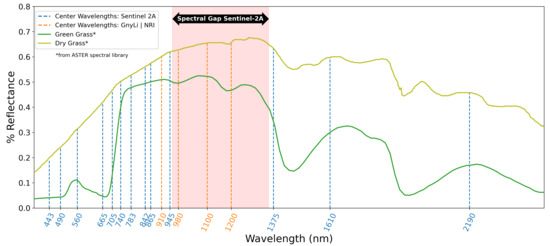
Figure 1.
Typical reflectance spectra for green and dry grass plotted from the ASTER spectral library [31], the center wavelengths of Sentinel-2A [32] (dashed vertical blue lines), and the applied center wavelengths of the VNIR/SWIR multi-camera system for the GnyLi and the NRI (dashed vertical orange lines).
According to Kumar et al. [28], the vegetation compounds’ spectral characteristics are present in this segment and are of interest for further investigations. Absorption minima caused by canopy moisture, cellulose, starch, and lignin can be found at around 970 and 1200 nm [28,29,30]. Reflectance maxima lie roughly at 910 and 1100 nm and are caused by components of protein content, lignin, and intercellular plant structures [28,29]. Roberts et al. [30] provide a detailed review on VIs for retrieving data on vegetation structure, canopy biochemistry, e.g., pigments or moisture, or plant physiology.
This study aims to evaluate and validate a novel VNIR/SWIR multi-camera system’s performance and potential to assess crop traits using a winter wheat field trial at the Campus Klein-Altendorf (North Rhine-Westphalia, Germany) as a case study. More specifically, the objectives are to (i) regress UAV-based and manually measured crop heights against ground truth data, (ii) apply resulting regression models to estimate crop traits (fresh and dry) biomass, crop moisture, NC, and N uptake, and (iii) evaluate and validate the relationship between NIR/SWIR-based vegetation indices and crop traits.
2. Study Site and Methods
2.1. Trial Description
Winter wheat was grown in an experimental field (50°37′11.85″N and 6°59′45.47″E) at the research site Campus Klein-Altendorf (CKA, www.cka.uni-bonn.de, last accessed on 4 March 2021), which is located near the City of Bonn, Germany. The CKA is the largest off-site laboratory experimental farm of the Faculty of Agriculture at the University of Bonn. The winter wheat trial is managed by the Institute of Crop Science and Resource Conservation (INRES, University of Bonn, Germany). The soil type can be described as a Haplic Luvisol on loess. The site is characterized by an Atlantic climate with a mean annual precipitation of 603 mm and a mean annual temperature of (1956–2020). The crops are grown under conventional management with regular application of pesticides, fungicides, and growth regulators. A crop rotation of winter barley–winter barley–sugar beet–winter wheat is maintained in the experimental field. At the time of sowing, the pH value averaged 6.7, and the humus content was 1.4%. Per 100 g of soil portion, P2O5 content was 20 mg, K2O content was 13 mg, and MgO content was 7 mg. Mineralized nitrogen (Nmin) content was 10 kg ha−1 at a soil depth of 0 to 30 cm, 32 kg ha−1 at 30 to 60 cm, and 18 kg ha−1 at 60 to 90 cm.
The winter wheat trial can be described as a split-plot design divided into five rows (see Figure 2). Each row is, in turn, subdivided into three nitrogen treatments (N1-N3). Each nitrogen treatment contains six different winter wheat varieties, first released in 1935 (see Table 1, [33]). On 11 November 2019, these varieties were randomly sown in plots measuring 7.0 × 1.5 m using a row spacing of 11.3 cm, resulting in a total number of 18 plots per row. Cultivars were grown under three different nitrogen levels, receiving either 0 (N1), 120 (N2), or 240 kg N ha−1 (N3). The 18 randomized crop-treatment combinations were replicated in the five rows, leading to 90 plots for the field trial. Nitrogen was supplied as calcium ammonium nitrate, with the first application during wheat tillering (17 March), the second at the beginning of stem elongation (16 April), and the third during the late booting stage (18 May) in 2020.
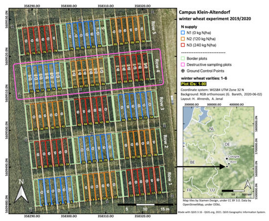
Figure 2.
Location map and additional information of the winter wheat experiment at Campus Klein-Altendorf (2019/2020).

Table 1.
Winter wheat varieties.
2.2. Biomass Sampling, Nitrogen Concentrations, and Height Measurements
Biomass sampling was performed destructively within one of the five rows (no. 4, see Figure 2) approximately every two weeks, resulting in a total number of six observation dates (8 April, 28 April, 13 May, 26 May, 9 June, and 2 July). During these observation dates, the complete plant biomass was cut using standard scissors at a length of 50 cm along three different sowing rows with three replicates for each plot. We excluded the two outermost rows from sampling to avoid edge effects. After measuring each sample’s fresh biomass (FBM) weight, sub-samples were oven-dried (at 105 for 1–2 days) to calculate the plant dry biomass (DBM) (g). The remaining plant biomass samples were oven-dried at 60 until reaching a constant weight and ground for the subsequent analysis of carbon (C) and NC (%) using a C/N analyzer (EuroEA3000, EuroVector S.p.A. (Italy)). Manual height measurements of all 90 plots were taken on the first five observation dates by holding a folding rule in the center of each plot and visually reading the crop height at the head of that plot.
2.3. UAV Data Acquisition for Crop Height Analysis—Crop Height Workflow
UAV-derived crop heights (CH) were produced using a DJI© Phantom 4 RTK (P4RTK). The P4RTK is equipped with a 1" global shutter CMOS sensor providing 20 megapixels in RGB. The P4RTK connects to an RTK base station for precise geotagging of the image data. Figure 3 displays the P4RTK during take-off, the base station, and the flown flight path pattern. The same flight plan was used for all UAV campaigns on nine dates: 26 March, 7 April, 28 April, 13 May, 26 May, 2 June, 12 June, 1 July, and 21 July. For each date, approx. 400 photos were acquired from a flight altitude of 25 above ground level (AGL). Besides the UAV data acquisition, 12 Ground Control Points (GCPs) were permanently installed and georeferenced with an RTK-GPS (Topcon GR-5).
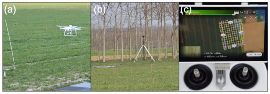
Figure 3.
The utilized UAV for crop height analysis is (a) a DJI© Phantom 4 RTK, which can be operated in RTK mode using (b) a base station. Flight planning is also possible (c).
Numerous studies have proven that UAV-derived image data for Structure from Motion and Multi-View Stereopsis (SfM/MVS) analysis provide a robust method to derive CH [17,34,35]. Therefore, we essentially followed the Crop Surface Model (CSM) approach introduced by Hoffmeister et al. [36] for terrestrial laser scanning data, which was successfully applied on a UAV data set for winter barley by Bendig et al. [16]. The latter used Agisoft Photoscan for SfM/MVS analysis to generate 3D data and Digital Orthophotos (DOPs). For this study, we used Metashape (Version 1.5.2, Agisoft LLC, St. Petersburg, Russia) for SfM/MVS analysis. We exported the DOPs and Digital Surface Models (DSMs) into ESRI’s ArcGIS software to compute CH from the DSMs. In this study, however, accounting for the suggestions by Lussem et al. [37], we tested a newly elaborated analysis workflow: (i) we used the direct RTK-georeferenced P4RTK images and batch-processed them directly in Metashape without using GCPs, (ii) we georeferenced DOPs and DSMs to the GCPs in ArcGIS, (iii) we normalized the elevation of all DSMs to the same take-off point of each UAV campaign in ArcGIS, and (iv) we computed crop heights in ArcGIS, subtracting the digital terrain model (DTM) from March 26 from all other dates. Step (iii) was intended and necessary due to appropriately setting the same x,y,z-data of the P4RTK base station on March 26 and April 28. The ground sampling distance was approx. for the DOPs and approx. for the DSMs. Figure 4 shows the DSM from 26 March, the CSM from June 12, and the CH, computed by subtracting the 26 March DSM from the 12 June CSM.
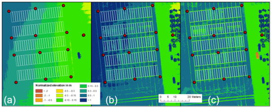
Figure 4.
Visualization of (a) the normalized base Digital Surface Model (DSM) at the beginning of the growing season 2020 on 26 March. In the middle, (b) represents a normalized Crop Surface Model (CSM) for 12 June, and (c) is the CH computed by subtracting (a) from (b).
2.4. VNIR/SWIR Imaging System and Vegetation Indices
This study’s evaluation applies a novel VNIR/SWIR multi-camera system [23], camSWIR. In a permanent grassland trial, Jenal et al. [38] successfully tested this prototype for its suitability in estimating forage mass. The system’s modular two-part design means it can be integrated into various aerial remote sensing platforms, focusing on UAV-based multi-rotor vehicles (see Figure 5). The centerpiece consists of the Spectral Camera Unit (SCU), which combines two VNIR enhanced SWIR cameras based on the semiconductor material InGaAs. Two single-wavelength image data sets are captured per flight. For this, each camera of the system is adopted with an application-specific bandpass filter via specially designed inter-changeable filter flanges to derive well-established VIs in the VNIR/SWIR spectral range.
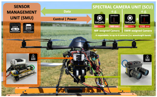
Figure 5.
Overview of the VNIR/SWIR multi-camera imaging system mounted on a UAV.
Table 2 summarizes the two NIR/SWIR-based VIs, GnyLi and NRI, which were chosen to evaluate the system’s spectral performance in this study. The four-band GnyLi was developed by Gnyp et al. [25] using hyperspectral narrow-band vegetation indices in winter wheat. This VI uses two local minima and maxima in the reflectance spectrum of vegetation between 900 and 1300 nm (see Figure 1). Absorption by canopy moisture, moisture stress, and plant water content dominate these two minima [30]. Overtone bands of starch (around 970 nm) as well as cellulose, starch, and lignin (around 1200 nm) also affect both absorption ranges [28,29,30]. The two reflectance maxima around 910 and 1100 nm are dominated by the plant leaves’ intercellular structures and to a minor extent by overtone bands of protein and lignin [28,29,39]. Thus, there are two biomass-related and two moisture-sensitive spectral components in the GnyLi equation.
Table 2.
NIR/SWIR vegetation indices derived from the camera system and used in this study. The wavebands used differ from the original selection of Gnyp et al. [25] and Koppe et al. [24], partly due to the limited range of readily available narrow-band and high-performance bandpass filters for this application.
In contrast to the bandpass wavelengths selected by Gnyp et al. [25], commercially available, narrow-band hybrid bandpass filters were selected at center wavelengths of 980 and 1200 nm for the reflectance minima and 910 and 1100 nm for the reflectance maxima, with a spectral bandwidth (full width-half maximum, FWHM) of (10 ± 2) nm each. This bandwidth already meets the spectral resolution, at least in the SWIR, of some hyperspectral sensors, especially in the field of EO satellite missions. A comprehensive overview can be found in Berger et al. [19].
The second VI uses an NDVI-like equation. This so-called normalized ration index (NRI) is widely used with different wavelengths, mainly in the VNIR domain [40,41]. Koppe et al. [24] extended this index to the NIR/SWIR range by empirical testing with Hyperion data and found high coefficients of determination between this narrow-band VI and above-ground biomass in winter wheat. In this study, the wavelengths of 910 and 1200 nm applied in the GnyLi VI were also used for the two-band NRI to cover the biomass and the moisture part of the winter wheat reflectance spectrum. A key advantage of both SWIR-based VIs over VNIR-based VIs, such as NDVI, is that they are not as susceptible to saturation issues due to increasing biomass density or leaf cover [42,43,44,45], which typically reaches nearly 100% in the mid-vegetative stage of crops [26]. As a result, it is possible to monitor the increasing amount of biomass beyond this stage.
2.5. Spectral Image Data Acquisition and Processing—Spectral Workflow
The camSWIR system acquired the spectral image data around noon on 2 June 2020. It took 28 min to perform two consecutive flights to collect the four necessary spectral bands. The first flight took off at 11:31 a.m. CET. Each flight lasted about 9 min. The remaining time was required for the bandpass-filter-equipped filter flange replacement and the corresponding camera calibration. During both flights, solar radiation conditions were stable and without any cloud coverage. The flight altitude of the UAV was set to 34 (AGL). In post-processing, the raw image data were flat-field-calibrated and converted from digital number (DN) to reflectance values using two different approaches, both based on the Empirical Line Method [46]. A simple workflow was performed via a one-point calibration with a series of images taken from a spectrally precisely characterized Zenith™ polymer white panel with 95% Lambertian reflectance before each flight. This white panel method is abbreviated as WPM in this study. The more complex variant involved six differently graded (0, 10, 25, 50, 75 and 100% black shading) near-Lambertian 80 × 80 cm gray panels positioned directly next to the experimental field. They were recorded several times during the UAV flights. These gray panels were then identified in five corresponding images for each waveband. Their averaged DN was determined (see Figure A3) by a Python script (version 3.7, Python Software Foundation) based on the roipoly module. A transfer function per wavelength channel was then calculated with these values (see Figure A2) and the grayscale panels’ reflectance data previously measured using ASD FieldSpec3 (Malvern Panalytical Ltd, Malvern, United Kingdom) (ASD). These functions were then used to convert the four DN image data sets to reflectance data. This workflow will be subsequently abbreviated as ELM. Additionally, for calibration purposes, a series of dark images were acquired before each flight. All post-processing steps were performed in the Python programming language using IPython [47] in a JupyterLab environment [48].
After calibration, each of the four reflectance image data sets for both calibration methods was processed separately in a photogrammetric software suite (Metashape v1.6.2, Agisoft LLC, St. Petersburg, Russia) to an orthomosaic. Coordinates of twelve permanent and evenly distributed ground control points (GCPs, see Figure 2) were used for precise georeferencing in Metashape. After processing, these eight single-waveband orthomosaics were used to derive two sets of GnyLi and NRI VI orthomosaics in QGIS (version 3.14, QGIS Association, www.qgis.org last accessed on 4 March 2021) for both calibration methods. Figure 6 shows an example of the two orthomosaics for the ELM calibration method. The averaged VI values for each plot were then extracted via the zonal statistics tool. These VI data sets could then be used to evaluate and validate the relationship between SWIR-based vegetation indices and crop traits in the subsequent regression analyses.
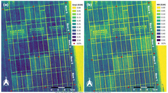
Figure 6.
(a) GnyLi and (b) NRI orthomosaics processed from the four ELM-calibrated waveband orthomosaics (910, 980, 1100 and 1200 nm) derived from the camera system’s spectral image data.
2.6. Crop Trait Estimation Workflow
A comprehensive analysis workflow was designed and performed to evaluate the new camSWIR system (see Section 2.4) for monitoring crop traits. Figure 7 gives an overview of the central data acquisition and analysis steps. The analysis workflow comprises six main data sets (I–VI) and one data set for validation, as described in the following.
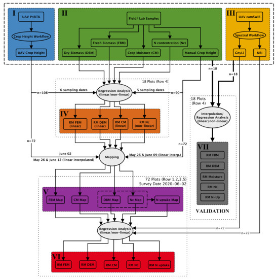
Figure 7.
Simplified scheme of the developed crop trait estimation workflow.
- (I)
- This data set represents the UAV data acquisition of RGB images using a P4RTK for stereo-photogrammetric analysis resulting in crop height data (UAV crop height). This part (crop height workflow) is described in detail above in Section 2.3, and these crop height data are of central importance for further data analysis.
- (II)
- In the field experiment, manual and destructive samplings of crop height and biomass were conducted. As described in Section 2.2, biomass was weighed before and after drying to determine fresh and dry biomass. The difference between fresh and dry biomass is considered the crop moisture content (crop moisture: CM). Dry biomass samplings were further analyzed for NC in the laboratory.
- (III)
- The third input data set for the analysis workflow originates from the newly developed camSWIR system flown on 2 June. The multi-camera system was optimized to derive two NIR/SWIR vegetation indices, the NRI and the GnyLi (compare Section 2.4). Section 2.5 describes the spectral workflow that transforms the raw DN image data sets into plot-wise VI reflectance data sets. For more details on the performance of the two VIs, see also [9,15,23,24,25,27,38].
- (IV)
- Regression models (RM) were created for the destructive field sampling plots (18 plots per date: n = 108) from (I) the UAV-derived crop height data and from (II) the manual and destructive sampling data, resulting in four regression models for biomass (fresh and dry), crop moisture, and NC. In Figure 8, the 108 sampling plots of Row 4 are shown. Each color represents a sampling date starting with orange for 8 April and ending with dark green for 2 July.
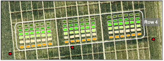 Figure 8. Image of 108 sampling plots (18 per date, color-coded).
 - (V)
- These four regression models from step (IV) were then applied to the remaining 7.0 × 1.5 m plots of Row 1, 2, 3, and 5 using the P4RTK CH data (I) as well as the manual CH data (II) as input. This approach allowed biomass (fresh and dry), crop moisture (CM), and NC to be estimated for the 72 test plots (18 per row). This step is possible because numerous studies have already proven the robustness of using CH as an estimator for biomass [49,50,51,52,53,54,55] and using biomass as an estimator for NC and N uptake [15,38,56]. With the derived data for dry biomass and NC, the N uptake could be calculated in line with Lemaire et al. [57] for the 72 test plots. Due to the abnormal UAV-derived crop heights for 2 June, an additional data set was generated by interpolating the UAV-derived crop height of 26 May and 12 June linearly for 2 June. This data set is named UAV crop height interpolated (P4RTK [i]).
- (VI)
- The camSWIR-based VIs (NRI and GnyLi) were regressed against the five crop traits (V). Regression coefficients were used to evaluate the camSWIR’s potential for monitoring crop traits.
- (VII)
- The proposed analysis workflow (I–VI) was validated by regression analyses of the five different field parameters (FBM, DBM, CM, NC, and N uptake) from the 18 destructive sampling plots and the two NIR/SWIR VIs, GnyLi, and NRI, considering two different spectral calibrations methods. Quality measures for better comparison were calculated (see Section 2.7). Again, the values for 2 June were linearly interpolated between the two sampling dates of 26 May and 12 June. The N uptake was derived from the 18 values of DBM and NC. In this validation, the sampled field and lab data were directly analyzed against the VIs.
2.7. Statistical Measures
To evaluate the estimation accuracy of the derived regression models, we calculated the coefficient of determination R2,
the root mean square error (RMSE),
and the normalized RMSE (NRMSE),
for a comprehensive comparison of the individual models [58]. Where is the ith estimated variable, is the ith observed variable by the RM, is the average of estimated variable x, and represents the average of observed variable y. The variable n specifies the number of elements in a data set.
3. Results
3.1. UAV Crop Height Data Evaluation
UAV-derived CH data sets (see Section 2.3) were used to estimate fresh and dry biomass, crop moisture, an indirect estimation of NC, and N uptake for the 72 non-destructively sampled plots of rows 1, 2, 3, and 5 (see Figure 7). Therefore, the UAV-derived CH data were evaluated using results from manual CH measurements (see Section 2.2). These manual measurements were performed on 8 April, 28 April, 13 May, 26 May, and 9 June for all 90 experimental field plots. UAV-based CH were significantly linearly correlated with manual CH for the five observation dates (R2 = 0.95, RMSE = 0.001, p < 0.001) (Figure 9a,b). This linear relation indicates that UAV-based CH can be accurately derived from UAV image data for the sampling plots (n = 90, Figure 9a). Additionally, the determined UAV CH for the remaining 72 plots (n = 360, Figure 9b) were also highly correlated to the respective manually measured CH values so that they could be used to estimate the five crop traits for each of the 72 plots (Figure 7 (V)).
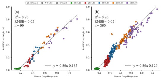
Figure 9.
(a) Scatter plot for the manually measured CH versus the UAV-based CH for the 18 destructive sampling plots for all five comparable dates. (b) Scatter plot for the manually measured CH versus the UAV-based CH for the remaining 72 test plots for all five comparable dates ( for all regression models).
The results of the CH analysis are shown for six dates in Figure 10. The figure shows that the derived CH data capture the winter wheat growing stages well and that “non-growing” objects such as foot- or driving paths are easy to recognize. Even the small, destructive sampling areas in Row 2 (compare Figure 2) are clearly recognizable. Detailed validation of the generated CH data is presented in Figure 9.
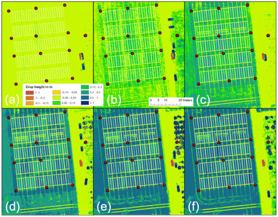
Figure 10.
UAV-derived development of crop height in meters over the growing season 2020 for (a) 7 April, (b) 28 April, (c) 13 May, (d) 26 May, (e) 12 June, and (f) 1 July.
An unexpected decrease in the UAV-derived CH was related to data obtained on 2 June, the UAV-based VNIR/SWIR data sampling date. This decrease is unrealistic and contrasts with all other data sets, indicating progressive plant growth throughout the growing season. Figure 11 shows the DOP and derived CH. Visually, the data look good, but detailed analysis shows a non-linear error, giving some plots an unrealistic drop in crop growth compared to that of 26 May. The latter represents an erroneous output of the methodology. A more in-depth analysis resulted in a systematic error for all plots of the zero N-input variants (N1). Figure 11a (also compare Figure 2) shows that these plots have a characteristic bright reflectance due to the lower vegetation cover.
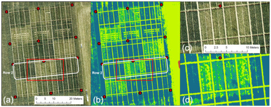
Figure 11.
UAV-derived CH data for 2 June (CH legend from Figure 4 applies): (a) DOP, (b) derived CH map, (c) enlarged area of DOP (red rectangle in (a), (d) enlarged area of CH map (red rectangle in (b).
Moreover, these are the plots that show the lowest CH in Figure 11b–d present an enlarged part of row 2, where the bright, almost outshining, soil reflectance of the N1 plots seems to dominate, resulting in false modeling of the ground instead of the crop canopy. As a consequence, the affected plant heights are modeled too shallowly. For 1 July, only variety no. 3 shows the same faulty behavior for the N1 fertilizer plots in all row replicates.
Further examination of all plot data for CH on 2 June confirms this finding. Firstly, in Figure 12, all CH values for all plots in Row 2 are plotted. The N2 and N3 N-variant plots show good and expected CH values, while all N1 plots show this significant decrease in crop growth, which is impossible. Secondly, a complete visualization of all CH data of rows 1, 2, 3, and 5 is displayed in Figure A1 in Appendix A. In particular, the N1 plot values show these significantly low CH values, with two exceptions included in Figure A1. Considering this effect, we used the data of 2 June with caution and created additionally a linearly interpolated, more realistic CH data set for 2 June using 26 May and 12 June data. This issue is addressed further in the discussion.
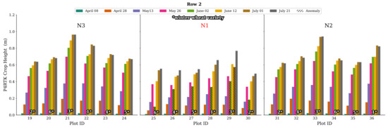
Figure 12.
Bar chart representation of CH derived by the UAV for row 2 for all flight dates. For all N1 treatment plots’ varieties, the crop height workflow resulted in an unexpected drop in plant growth for 2 June. This phenomenon is also evident in all N1 stages of the other rows (see Figure A1). Variety no. 3 also shows negative growth for 1 July for all N1 treatments. The corresponding erroneous crop height values are marked with a hatched overlay in black.
3.2. Crop Traits Estimation Models
Regression fits between FBM, DBM, and CM with UAV-based (Figure 13a,d,g) and manually measured (Figure 13b,e,h) CH indicate a statistically significant linear relation. In contrast, as shown in Figure 13c,f,i, there was a non-linear decrease in NC over the growing season. This curve shape is also known as the nitrogen dilution effect and is best described by a power function [59]. Therefore, three non-linear regression models, based on a power-law fit, for estimating NC were derived from FBM, DBM, and CM (see Section 3.4 for further details).
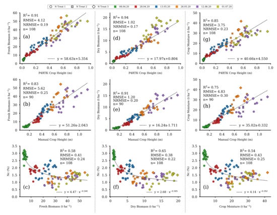
Figure 13.
Scatter plots of the linear regression models for P4RTK and manual CH against the fresh and dry biomass as well as crop moisture data of the 18 destructive sampling plots for the five and six sampling dates, respectively. Each column contains a non-linear regression model for estimating NC from the three different biomass parameters. Left column: regression models for fresh biomass (a–c). Center column: regression models for dry biomass (d–f). Right column: regression models for crop moisture (g–i). ( for all regression models).
Accuracy measures indicate lower errors and higher regression coefficients for model-based estimates of FBM, DBM, and CM if they are based on UAV-derived CH compared with those based on manually measured CH data (Table 3).
Table 3.
Regression performance results for the estimation models for fresh (FBM) and dry biomass (DBM), crop moisture (CM) and N concentration (NC) against UAV-based and manually measured CH data. ( for all regression models).
3.3. Regression Analyses of Vegetation Indices and Biomass
Based on the regression models from Section 3.2 derived from the 18 destructive sampling plots, the respective data were estimated for the remaining 72 test plots. These data sets were then used in a further step to evaluate the VI data sets of the GnyLi and the NRI (ELM and WPM calibration) as estimators. Since the three biomass models (fresh, dry, moisture) are based on CH as the estimator, the biomass data sets were derived using three different CH data sets for the survey on 2 June. The first data set is the CH determined by the P4RTK image data on 2 June. However, due to the erroneous height data, the CH from two dates specified to be correct (26 May and 12 June) were linearly interpolated for 2 June and used in the model to estimate the biomass parameters. Since CH data for 2 June was also not available for the manual measurement, these data were also linearly interpolated from the two manual CH data sets (26 May and 9 June) and then used to estimate the values for FBM, DBM, and CM for the remaining 72 test plots. In combination with the four VI data sets, this resulted in twelve models for each biomass parameter. Figure 14 displays the twelve plots for the FBM data sets estimated by the three different CH data sets. The best-performing CH data set seems to be from 2 June (left column) with an R2 of 0.75 to 0.77 throughout all parameters. However, the RMSE is significantly reduced by more than 20% compared to the P4RTK-based models and less than 15% to the manual-height-based models. Since these data are considered erroneous (see Section 3.1), they are included for completeness only.
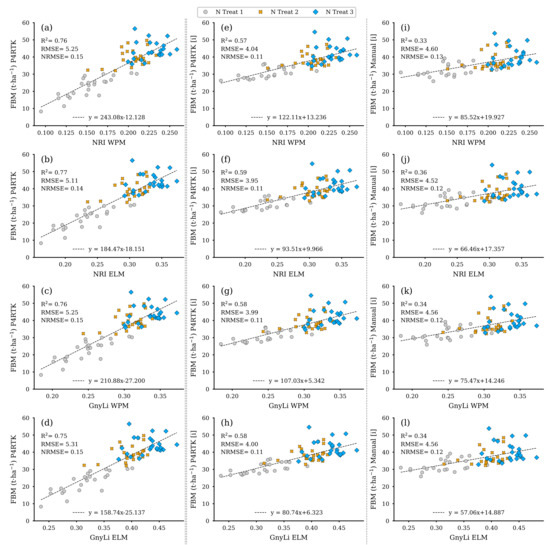
Figure 14.
Scatter plots for the fresh biomass (FBM) data estimated for the 72 non-destructive test plots with the FBM-model based on three different crop height data sets with the spectral camera VIs acquired on 2 June. Left column: crop height directly derived from P4RTK RGB data set of 2 June (a–d). Center column: linear interpolated crop height from P4RTK RGB data set of 26 May and 12 June (e–h). Right column: linear interpolated crop height manually measured on 26 May and 9 June (i–l). ( for all regression models).
The center and right columns of Figure 14 present the scatter plots for the FBM derived from the interpolated CH data (P4RTK, manual) and the two VIs with both calibration methods. It can be seen that the FBM values derived from the P4RTK CH data (center) with an R2 of 0.57 to 0.59 are considerably more accurate than the FBM values based on the manually measured CH (right column) with an R2 of 0.33 to 0.36. Additionally, the UAV-based regression models have the lowest RMSE 3.95 to 4.04 t ha−1 and NRMSE (11%) values. More significant errors are mainly linked to the plots receiving greater nitrogen amounts (N3, blue diamond markers).
Figure 15 displays, like Figure 14, the models for the VIs as estimators, but here for the dry biomass (DBM) estimated from the three different CH data sets for the remaining 72 test plots. Due to the underlying relationship of CH as the joint estimator, these models exhibit similar performance behavior to those shown in Figure 14, even compared to each other. The left column again shows the co-incidence of the VIs with the erroneous CH data from 2 June with a better R2 compared to the other two models based on interpolated CH values.
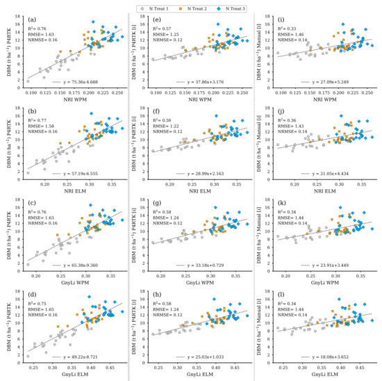
Figure 15.
Scatter plots for the dry biomass (DBM) data estimated for the 72 non-destructive test plots with the DBM-model based on three different CH data sets with the spectral camera VIs acquired on 2 June. Left column: CH directly derived from P4RTK RGB data set of 2 June (a–d). Center column: linearly interpolated CH from P4RTK RGB data set of 26 May and 12 June (e–h). Right column: linearly interpolated CH manually measured on 26 May and 9 June (i–l). ( for all regression models).
Figure 16 shows the resulting regression models based on both VIs as crop moisture estimators. Since crop moisture is directly related to wet and dry biomass, the performance of these models is almost identical to the models shown in Figure 14 and Figure 15 but again in a different magnitude relationship. Table 4 summarizes the regression analyses’ results for the three parameters FBM, DBM, and CM.
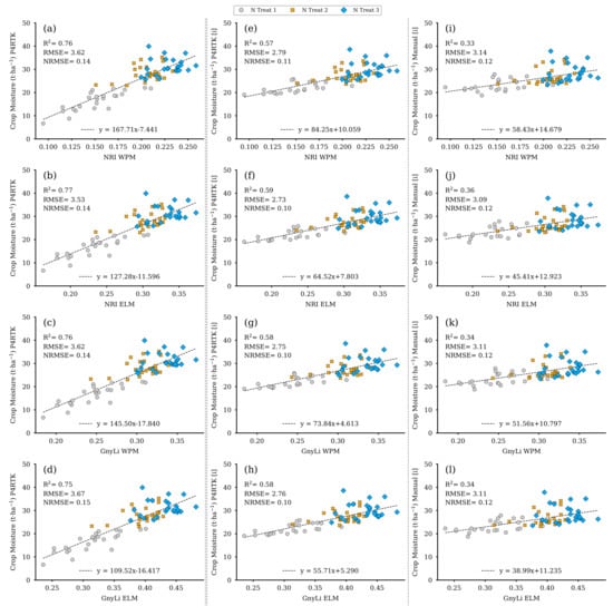
Figure 16.
Scatter plots for the crop moisture (CM) data were estimated for the 72 non-destructive test plots with the CM model based on three different CH data sets with the spectral camera VIs acquired on 2 June. Left column: CH directly derived from P4RTK RGB data set of 2 June (a–d). Center column: linear interpolated CH from P4RTK RGB data set of 26 May and 12 June (e–h). Right column: linear interpolated CH manually measured on May 26 and 9 June (i–l). ( for all regression models).
Table 4.
Results of the linear regression analyses for both calibration methods (WPM, ELM) of both VIs (G: GnyLi, N: NRI) and the estimated (by three different CH) crop traits: fresh and dry biomass and the crop moisture. Three CH: P4: P4RTK crop height, M: manual crop height, [i]: interpolated crop height values. ( for all regression models).
3.4. Regression Analyses of Vegetation Indices and NC and N uptake
As shown in Figure 13f, the best predictor for NC was DBM. The corresponding non-linear regression model had the highest R2 of 0.65 and the lowest RMSE of 0.38 compared to the RM based on FBM (R2: 0.58, RMSE: 0.41) or CM (R2: 0.54, RMSE: 0.43). Since the DBM was estimated with three different CH data sets, as shown in Section 3.3, this also resulted in three data sets for the estimated NC. These data sets were then finally further investigated with regression analyses, with the two VIs, GnyLi, and NRI (WPM, ELM), as estimators. Again, this results in twelve regression models for the flight date on 2 June, shown in Figure 17. The equations exhibit a negative slope. This phenomenon resulted from the decrease in NC with an advanced plant growth state for the N2 and N3 plots but not for the zero-fertilization N1 plots.
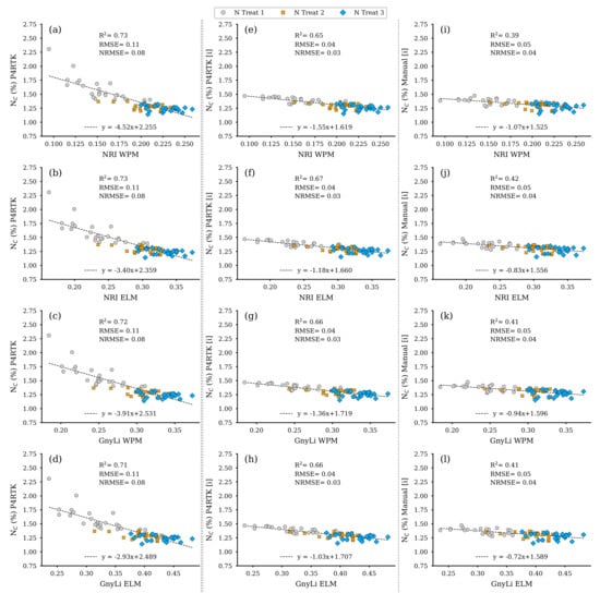
Figure 17.
Scatter plots for the N concentration (NC) data estimated for the 72 non-destructive test plots with the NC-model, based on the DBM estimator RM for three different CH data sets, with the spectral camera VIs acquired on 2 June. Left column: CH directly derived from P4RTK RGB data set of 2 June (a–d). Center column: linear interpolated CH from P4RTK RGB data set of 26 May and 12 June (e–h). Right column: linear interpolated CH manually measured on 26 May and 9 June (i–l). ( for all regression models).
The regression models based on the erroneous CH data from the RGB image data acquired on 2 June appear to perform well, as in the previous analyses, with R2 of 0.71 to 0.73. However, they should be considered as an artifact. Compared to the results with the interpolated CH data from Section 3.3, the analysis data for the VIs estimators for the UAV-based NC estimators are better, with R2 of 0.65 to 0.67, than the comparable estimators for biomass (see Figure 14, Figure 15 and Figure 16). The regression models based on the VIs and the NC estimated with the manually measured CH data again perform weakest, with an R2 of 0.39 to 0.42 (Table 5). These results are slightly higher than the regression analyses of the VIs and the biomass parameters (Section 3.3). The RMSE for the estimated NC based on interpolated CH data sets (P4RTK, Manual) is comparatively low.
Table 5.
Results of the simple linear regression analyses for both calibration methods (ELM, WPM) of both VIs (NRI, GnyLi) and the estimated (by three different CH) crop traits: NC and N uptake. Three crop heights: P4: P4RTK crop height, M: manual crop height, [i]: interpolated crop height values. ( for all regression models).
Figure 18 shows the regression analysis results for N uptake using the two VIs, GnyLi and NRI (WPM, ELM), as estimators. The N uptake was calculated from the values for DBM and NC of the 72 test plots. These two features were also derived using the established regression models from Section 3.2 and the three different CH for the 2 June survey date. Each CH-related model is arranged in its corresponding column in Figure 18.
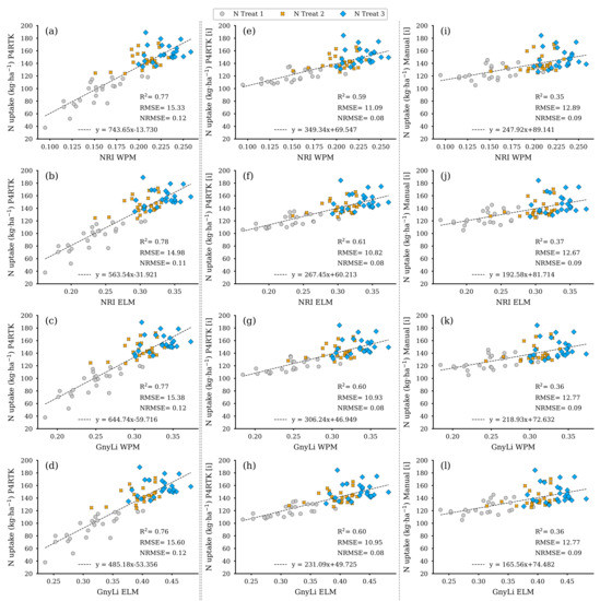
Figure 18.
Scatter plots for the N uptake data estimated for the 72 non-destructive test plots with the NC and DBM RM-model, based on the DBM estimator RM for three different CH data sets, with the spectral camera VIs acquired on 2 June. Left column: CH directly derived for 2 June P4RTK RGB data set (a–d). Center column: linear interpolated CH from 26 May and June 12 P4RTK RGB data sets (e–h). Right column: linear interpolated CH manually measured on 26 May and 9 June (i–l). ( for all regression models).
3.5. Regression Analyses of Vegetation Indices and Ground Truth Data
To validate the results from the previous regression analyses (compare Section 2.6, step VI), the spectral information of the two VIs, GnyLi, and NRI (ELM, WPM), was derived from the remaining standing biomass in the 18 destructive samplings plots on 2 June (see Figure 7, dark green and previous sampling area). These four VI data sets were then analyzed with the linearly interpolated ground truth data sets of May 26 and June 12 from these plots in simple linear regression models. Figure 19 shows the scatter plots of the individual analyses of the VIs as an estimator for the ground truth data of FBM, DBM, CM, NC, and N uptake. As explained in Section 2.6, CM was derived from FBM and DBM, and the N uptake was processed from Nc and DBM. The results consistently show a high R2 of at least 0.73 to a maximum of 0.87. Table 6 summarizes the particular linear regression results for each VI as an estimator for the respective crop trait.
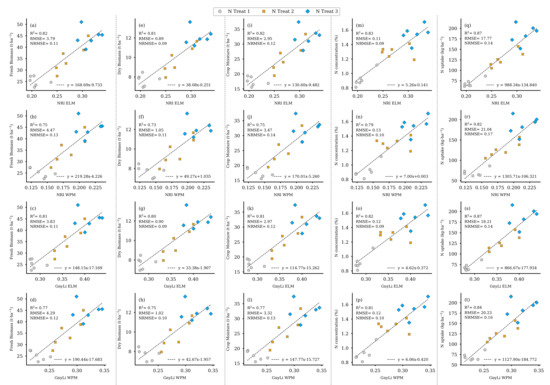
Figure 19.
Scatter plots for the VI data for 2 June as estimators for the individual crop traits linearly interpolated from 26 May and 12 June of the 18 destructive sampling plots. (a–d) camSWIR VIs and FBM, (e–h) camSWIR VIs and DBM, (i–l) camSWIR VIs and crop moisture, (m–p) camSWIR VIs and NC, (q–t) camSWIR VIs and N uptake. ( for all regression models).
Table 6.
Regression analyses’ results for the VIs as estimators for the sampled ground truth data (FBM: fresh biomass, DBM: dry biomass, NC: N concentration, CM: crop moisture, NUP: N uptake) of the 18 destructive sample plots. ( for all regression models).
4. Discussion
In this study, a newly developed VNIR/SWIR imaging system for UAVs, the camSWIR, is evaluated for crop trait monitoring of winter wheat. The focus is on two vegetation indices (VIs), the NRI [24] and the GnyLi [25], which used near and short-wave infrared (NIR/SWIR) wavelengths (see Table 2). Previous studies showed that these indices outperformed VIs using bands from the visible and near-infrared (VIS/NIR) domain [9,24,25,26,38,56,60]. Moreover, several authors indicate the SWIR domain’s potential for crop trait monitoring [15,19,30,61,62,63,64].
The presented results in this case study for winter wheat demonstrate this new sensor’s potential to derive crop traits such as biomass, NC, N uptake, and crop moisture. Although not typically used, these wavelengths’ potential for monitoring agricultural systems has also been shown in other studies. For example, Ceccato et al. [65] indicate the SWIR domain’s potential to derive leaf water content. Honkavaara et al. [66] indicate the same for monitoring surface moisture of a peat production area. Camino et al. [27] demonstrated the advantage of the SWIR domain for retrieval of crop nitrogen. Finally, Psomas et al. [67] and Koppe et al. [24] proved the NIR/SWIR bands’ suitability for biomass monitoring in grasslands and winter wheat. The selection of the applied bandpass filters in this study represents a compromise due to availability and cost compared to the original studies by Koppe et al. [24] and Gnyp et al. [25], which used field spectroradiometer and hyperspectral satellite data. If available in future studies, narrower (< 10 nm), more wavelength-specific, bandpass filters should be used to investigate an effect on the estimation performance of the VIs with the wavelengths applied in [24,25]. In particular, when it comes to spectral features involving leaf chemicals such as proteins that also have an indirect link to NC, using narrow-band filters with the appropriate center wavelengths [29,68] is crucial. Otherwise, when broader bandwidths are applied, this information about the fine spectral features is lost in the superimposed spectrum [69]. Furthermore, water absorption has to be considered as it overlays all other features to a large extent in the SWIR domain [64].
The NRI and GnyLi performed well as an estimator for different crop traits for the 72 test plots (Figure 7, step V and VI) in our study. In a first approach, we calculated comparatively high R2 values (NRI, GynLi) for FBM (R2: 0.77, 0.75), DBM (R2: 0.77, 0.75), NC (R2: 0.73, 0.71), N uptake (R2: 0.78, 0.76), and crop moisture (R2: 0.77, 0.75) with low NRMSEs ranging from 8 to 16%. However, these good results for one date (2 June) result from a supposed spurious effect in the P4RTK RGB image data processed in the crop height workflow described in Section 2.3. The low vegetation cover in the N1-treatment where nitrogen supply was omitted caused a significant CH error in the SfM/MVS analysis. This effect is most likely due to the strong reflectance of the high soil coverage and should be further investigated in the future. However, for all other observation dates, the P4RTK image data tracks crop growth with high accuracy (R2: 0.95 for the 18 destructive sampling plots and R2: 0.95 for the remaining 72 test plots) compared to the crop heights measured by hand with a folding ruler. The RMSE of is within the expected resolution for stereo-photogrammetric height measurement from image data for both regression models (see Figure 9).
To avoid the negative effect in the CH data, a second validation data set was produced by linearly interpolating the CH for 2 June to provide more reliable CH data. The regression models based on this interpolated data set resulted in moderately lower R2 values for FBM (R2: 0.59, 0.58), dry DBM (R2: 0.59, 0.58), NC (R2: 0.67, 0.66), N uptake (R2: 0.61, 0.60), and crop moisture (R2: 0.59, 0.58). A reduction in RMSE (more than 20%) and NRMSE (4 percentage points) was also observed in the regression models of the interpolated data sets. Thus, while the variability in crop traits explained by the model was lower, absolute and mean-normalized prediction errors decreased. This decrease was mainly due to lower errors for predicting crop traits in the N1 treatment (see Figure 14, Figure 15, Figure 16, Figure 17 and Figure 18).
Compared to these findings, the regression analysis results used to validate both VIs using the ground-truth-based crop traits data from the 18 destructively sampled plots (see Figure 2 and Figure 7 step VII) consistently showed an even higher accuracy, ranging from R2: 0.73 to R2: 0.87, and lower RMSE values. This difference originates from a weaker correlation between UAV-derived CH data, which are the base for estimating the crop traits of the 72 test plots for 2 June. Therefore, this slightly weaker correlation affects the estimation accuracy of the final step of the crop trait estimation workflow (Figure 7 step VI), in which the UAV-derived crop traits are estimated using the VIs in regression models. In contrast, the base regression models of the destructively derived crop traits for all sampling dates performed better (see Figure 13) with the UAV-derived CH (R2: 0.54 to 0.94). Based on these CH, crop traits were estimated in turn for regression analyses with the VIs for the remaining 72 test plots. This slightly weaker relationship affects the last analysis step’s estimation accuracy (Figure 7 step VI).
The same relationship can be observed in the regression analyses based on the manually measured CH. The comparison of the two CH data sets’ performance revealed significant differences in estimation accuracy related to the VIs, whereby the crop traits’ regression models based on the manually measured CH performs worse (R2: 0.33 to 0.42) than the P4RTK-based crop traits (R2: 0.57 to 0.67). This difference is described by Bareth et al. [70]. It occurs because UAV-derived CH data, unlike point-wise manually measured ones, represent a mean plant height value of an entire plot accounting for the plant density resulting from zonal statistics. Another solution to provide CH data for reliably estimating crop traits might be utilizing UAV-LiDAR data [71,72,73] and should be investigated in future research.
Li et al. [45] investigated the performance of established VIs and tested for optimal wavelength combinations in the VIS/NIR domain to retrieve NC for certain growing stages. In their study on winter wheat, the authors found that all of the 77 published VIs and the best waveband combinations performed poorly (R2 < 0.29). Similar results are described by Mistele et al. [74] for maize. Gnyp et al. [75] investigated field spectra in rice and found similar moderate to poor R2 when applying VIs across all growing stages (R2 < 0.5). Reaching a higher R2 of up to 0.8 was only possible by using step-wise multiple linear regression (MLR) or narrow NIR/SWIR bands for the complete data set summarizing all growing stages. Stroppiana et al. [20] present similar results from several studies, showing moderate to low R2 for N retrieval for distinct growing stages. In general, most studies report only moderate to poor R2 for a single survey date. Thus, the ability of VIs in the VIS/NIR domain to estimate crop NC is limited. In particular, this applies to studies based on single survey dates. Considering the results from this study, we, therefore, suggest evaluating in more detail the performance of systems operating in the SWIR domain in future studies on date-specific crop trait estimation.
The results show that the recently introduced imaging system produces reliable VNIR/SWIR image data for the four selected wavebands. While only grayscale panels, destructively sampled crop data and estimated crop traits based on CH data could be used in this study, Jenal et al. [38] additionally used field-spectroradiometer measurements (350 to 2500 nm) of grassland canopies. In the latter study, very high correlations between both independent reflectance data sets have already been demonstrated. In this study, the spectral quality of the image data was shown again, and similar excellent results were produced for the grayscale panel calibration (ELM) method (Figure A2) as described in [38]. In determining the panel reflectances in the WPM-calibrated images (Figure A3) and regressing them with the panel reflectances, the quality of the WPM calibration method was successfully tested (Figure A4). The easy-to-use calibrated VNIR/SWIR spectral image data sets could be processed to derive plot-specific vegetation index reflectance values. An appropriate methodology was elaborated in previous studies [23,38]. The high sensitivity over almost the entire NIR/SWIR range of the InGaAs sensors used provides a high signal-to-noise ratio, which is crucial according to Stroppiana et al. [20], and such sensors are a missing technology for crop trait monitoring. NIR-enhanced silicon-based VIS imagers are mainly affected by this issue due to a drop in sensitivity at their spectral detection limits. However, non-enhanced InGaAs sensors (900 to 1700 nm) also reach their spectral limits in the NIR, with steep sensitivity drops at both spectral ends. For this reason, VIS-NIR-enhanced InGaAs sensors (600 to 1700 nm) have advantages as they partially overcome these problems, especially in the NIR/SWIR domain.
Comparing the tested image reflectance calibration techniques (ELM and WPM, see Section 2.5), both performed similarly (Table 4, Table 5 and Table 6), with slight differences in R2 values dependent on the data set but not systematic. Thus, distinct recommendations on specific index-calibration method combinations could not be identified. This observation is again consistent with the findings of Jenal et al. [38].
5. Conclusions and Outlook
The results presented in this study indicate that the VNIR/SWIR multi-camera system camSWIR is suitable for acquiring spectral image data in the NIR/SWIR. The derived vegetation indices were demonstrated to be capable of estimating agronomic relevant crop traits in winter wheat. In comparison with destructively measured crop trait data, both tested VIs (GnyLi and NRI) reached high estimation accuracies (R2: 0.73 to 0.87) in the regression models for validation.
The findings of this study further imply that by applying the proposed multilevel crop trait estimation workflow, biomass-related crop traits can be estimated in regression models using SfM/MVS-derived CH data from UAV RGB imagery. Such applications are beneficial for a reliable assessment of crop traits using UAV data since the availability of ground truth data is most often the limiting factor. In this study, this workflow’s implementation led to bivariate regression models based on both NIR/SWIR VIs and the estimated crop traits, based on UAV-derived crop heights, which reached high accuracies (R2: 0.57 to 0.67).
The CH data for 2 June, which were considered unrealistic since they suggested a drop in the seasonal crop height development, raise the intriguing research question of this method’s limitations. Therefore, this phenomenon requires further investigation and methodological improvements in order to avoid compromising effects. Alternatively, CH derived from UAV LiDAR data should also be investigated.
The results presented here are based on data from a single observation data. Thus they are noteworthy but not yet representative and need to be confirmed by further studies. Future evaluations of the camSWIR imaging system using multi-temporal and multi-year data acquisition campaigns on a winter wheat field trial are planned. To allow for a comparison with established methods, such evaluations optimally also include data from airborne VNIR imaging systems and spectral ground truth using a portable spectroradiometer in the field.
Given that future evaluations confirm the results of this study, spectral data collected by the VNIR/SWIR multi-camera system can provide additional information for more accurate yield estimation or efficient fertilizer management in precision agriculture.
Author Contributions
Conceptualization, G.B. and A.J.; methodology, A.J.; validation, H.E.A., A.B. and A.J.; formal analysis, A.J. and G.B.; investigation, A.J., H.E.A., A.B., G.B., and H.H.; data curation, A.J.; visualization, A.J.; writing–original draft preparation, A.J. and G.B.; writing–review and editing, H.E.A., A.B., H.H., and J.B.; supervision, G.B., H.H., and J.B.; funding acquisition, G.B. and J.B. All authors have read and agreed to the published version of the manuscript.
Funding
This research was partly funded by the Federal Ministry of Education and Research (BMBF) [Grant number 031B0734F] as part of the consortium research project “GreenGrass”.
Acknowledgments
The authors would like to thank the technical staff of Campus Klein-Altendorf for handling the experimental field throughout the growing season from seeding to harvest.
Conflicts of Interest
The authors declare no conflict of interest.
Appendix A. P4RTK Crop Height - Bar Plots

Figure A1.
Graphical visualization of CH values for all relevant flight dates and all winter wheat varieties of rows 1, 2, 3, and 5 of the experimental field. The unexpectedly derived negative plant growth for the 2 June flight date by the crop height workflow is mainly found in the N1 plots, with three exceptions. Another noticeable phenomenon is the drop-in crop growth of variety no. 3 in all N1 stages of flight date 1 July. The corresponding erroneous CH values are marked with a hatched overlay in black.

Appendix B. Reflectance Calibration by Grayscale Panels (ELM)

Figure A2.
Regression analyses of the grayscale panel DN values measured in the flat-field corrected image data and the reflectance of the gray panels, measured by a portable ASD FieldSpec3 spectroradiometer (Malvern Panalytical Ltd, Malvern, United Kingdom) (ASD). For each of the four wavelength bands (a–d), five images were analyzed, and the resulting DNs of the respective gray panels were averaged. ( for all regression models).

Appendix C. WPM Calibration Method Test

Figure A3.
Last step of a developed Python script to determine the averaged pixel values of selected areas. Here the resulting grayscale panels’ reflectance values for one WPM-calibrated image are displayed. The same script is used when determining the average digital numbers of the grayscale panels in the flat-field calibrated images for deriving the transfer function for converting the DN to reflectance values.


Figure A4.
Regression analyses of the gray panel reflectance values in the WPM-calibrated images and the reflectance of the gray panels, measured by a portable ASD FieldSpec3 spectroradiometer (Malvern Panalytical Ltd, Malvern, United Kingdom) (ASD). For each of the four wavelength bands (a–d), five images were analyzed, and the resulting reflectance of the respective gray panel was averaged. ( for all regression models).

References
- Foley, J.A.; Ramankutty, N.; Brauman, K.A.; Cassidy, E.S.; Gerber, J.S.; Johnston, M.; Mueller, N.D.; O’Connell, C.; Ray, D.K.; West, P.C.; et al. Solutions for a Cultivated Planet. Nature 2011, 478, 337–342. [Google Scholar] [CrossRef] [PubMed]
- Huang, S.; Miao, Y.; Yuan, F.; Gnyp, M.L.; Yao, Y.; Cao, Q.; Wang, H.; Lenz-Wiedemann, V.I.S.; Bareth, G. Potential of RapidEye and WorldView-2 Satellite Data for Improving Rice Nitrogen Status Monitoring at Different Growth Stages. Remote Sens. 2017, 9, 227. [Google Scholar] [CrossRef]
- Weiss, M.; Jacob, F.; Duveiller, G. Remote Sensing for Agricultural Applications: A Meta-Review. Remote Sens. Environ. 2020, 236, 111402. [Google Scholar] [CrossRef]
- Atzberger, C. Advances in Remote Sensing of Agriculture: Context Description, Existing Operational Monitoring Systems and Major Information Needs. Remote Sens. 2013, 5, 949–981. [Google Scholar] [CrossRef]
- Mulla, D.J. Twenty Five Years of Remote Sensing in Precision Agriculture: Key Advances and Remaining Knowledge Gaps. Biosyst. Eng. 2013, 114, 358–371. [Google Scholar] [CrossRef]
- Veloso, A.; Mermoz, S.; Bouvet, A.; Le Toan, T.; Planells, M.; Dejoux, J.F.; Ceschia, E. Understanding the Temporal Behavior of Crops Using Sentinel-1 and Sentinel-2-like Data for Agricultural Applications. Remote Sens. Environ. 2017, 199, 415–426. [Google Scholar] [CrossRef]
- Hütt, C.; Waldhoff, G.; Bareth, G. Fusion of Sentinel-1 with Official Topographic and Cadastral Geodata for Crop-Type Enriched LULC Mapping Using FOSS and Open Data. ISPRS Int. J. Geo-Inf. 2020, 9, 120. [Google Scholar] [CrossRef]
- Aasen, H.; Burkart, A.; Bolten, A.; Bareth, G. Generating 3D Hyperspectral Information with Lightweight UAV Snapshot Cameras for Vegetation Monitoring: From Camera Calibration to Quality Assurance. ISPRS J. Photogramm. Remote Sens. 2015, 108, 245–259. [Google Scholar] [CrossRef]
- Bendig, J.; Yu, K.; Aasen, H.; Bolten, A.; Bennertz, S.; Broscheit, J.; Gnyp, M.L.; Bareth, G. Combining UAV-Based Plant Height from Crop Surface Models, Visible, and near Infrared Vegetation Indices for Biomass Monitoring in Barley. Int. J. Appl. Earth Obs. Geoinf. 2015, 39, 79–87. [Google Scholar] [CrossRef]
- Candiago, S.; Remondino, F.; De Giglio, M.; Dubbini, M.; Gattelli, M. Evaluating Multispectral Images and Vegetation Indices for Precision Farming Applications from UAV Images. Remote Sens. 2015, 7, 4026–4047. [Google Scholar] [CrossRef]
- ten Harkel, J.; Bartholomeus, H.; Kooistra, L. Biomass and Crop Height Estimation of Different Crops Using UAV-Based Lidar. Remote Sens. 2020, 12, 17. [Google Scholar] [CrossRef]
- Sagan, V.; Maimaitijiang, M.; Sidike, P.; Eblimit, K.; Peterson, K.T.; Hartling, S.; Esposito, F.; Khanal, K.; Newcomb, M.; Pauli, D.; et al. UAV-Based High Resolution Thermal Imaging for Vegetation Monitoring, and Plant Phenotyping Using ICI 8640 P, FLIR Vue ProR 640, and thermoMap Cameras. Remote Sens. 2019, 11, 330. [Google Scholar] [CrossRef]
- Bareth, G.; Bolten, A.; Bendig, J. Potentials for Low-Cost Mini-UAVs. In Proceedings of the Workshop of Remote Sensing Methods for Change Detection and Process Modelling, University of Cologne, Cologne, Germany, 18–19 November 2010; pp. 1–8. [Google Scholar] [CrossRef]
- Maes, W.H.; Steppe, K. Perspectives for Remote Sensing with Unmanned Aerial Vehicles in Precision Agriculture. Trends Plant Sci. 2019, 24, 152–164. [Google Scholar] [CrossRef]
- Aasen, H.; Bareth, G. Spectral and 3D Nonspectral Approaches to Crop Trait Estimation Using Ground and UAV Sensing. In Hyperspectral Remote Sensing of Vegetation, 2nd ed.; Thenkabail, P.S., Lyon, G., Huete, A., Eds.; CRC Press Taylor & Francis Group: Boca Raton, FL, USA, 2018; Volume III, Title: Biophysical and Biochemical Characterization and Plant Species Studies; pp. 103–131. [Google Scholar] [CrossRef]
- Bendig, J.; Bolten, A.; Bareth, G. UAV-Based Imaging for Multi-Temporal, Very High Resolution Crop Surface Models to Monitor Crop Growth VariabilityMonitoring Des Pflanzenwachstums Mit Hilfe Multitemporaler Und Hoch Auflösender Oberflächenmodelle von Getreidebeständen Auf Basis von Bildern Aus UAV-Befliegungen. Photogramm.-Fernerkund.-Geoinf. 2013, 2013, 551–562. [Google Scholar] [CrossRef]
- Bareth, G.; Schellberg, J. Replacing Manual Rising Plate Meter Measurements with Low-Cost UAV-Derived Sward Height Data in Grasslands for Spatial Monitoring. PFG J. Photogramm. Remote Sens. Geoinf. Sci. 2018, 86, 157–168. [Google Scholar] [CrossRef]
- Gilliot, J.M.; Michelin, J.; Hadjard, D.; Houot, S. An Accurate Method for Predicting Spatial Variability of Maize Yield from UAV-Based Plant Height Estimation: A Tool for Monitoring Agronomic Field Experiments. Precis. Agric. 2020. [Google Scholar] [CrossRef]
- Berger, K.; Verrelst, J.; Féret, J.B.; Wang, Z.; Wocher, M.; Strathmann, M.; Danner, M.; Mauser, W.; Hank, T. Crop Nitrogen Monitoring: Recent Progress and Principal Developments in the Context of Imaging Spectroscopy Missions. Remote Sens. Environ. 2020, 242, 111758. [Google Scholar] [CrossRef]
- Stroppiana, D.; Fava, F.; Boschetti, M.; Brivio, P.A. Estimation of Nitrogen Content in Herbaceous Plants Using Hyperspectral Vegetation Indices. In Hyperspectral Indices and Image Classifications for Agriculture and Vegetation; CRC Press: Boca Raton, FL, USA, 2018. [Google Scholar] [CrossRef]
- Herrmann, I.; Karnieli, A.; Bonfil, D.J.; Cohen, Y.; Alchanatis, V. SWIR-Based Spectral Indices for Assessing Nitrogen Content in Potato Fields. Int. J. Remote Sens. 2010, 31, 5127–5143. [Google Scholar] [CrossRef]
- Kandylakis, Z.; Falagas, A.; Karakizi, C.; Karantzalos, K. Water Stress Estimation in Vineyards from Aerial SWIR and Multispectral UAV Data. Remote Sens. 2020, 12, 2499. [Google Scholar] [CrossRef]
- Jenal, A.; Bareth, G.; Bolten, A.; Kneer, C.; Weber, I.; Bongartz, J. Development of a VNIR/SWIR Multispectral Imaging System for Vegetation Monitoring with Unmanned Aerial Vehicles. Sensors 2019, 19, 5507. [Google Scholar] [CrossRef]
- Koppe, W.; Li, F.; Gnyp, M.L.; Miao, Y.; Jia, L.; Chen, X.; Zhang, F.; Bareth, G. Evaluating Multispectral and Hyperspectral Satellite Remote Sensing Data for Estimating Winter Wheat Growth Parameters at Regional Scale in the North China Plain. Photogramm.-Fernerkund.-Geoinf. 2010, 2010, 167–178. [Google Scholar] [CrossRef]
- Gnyp, M.L.; Bareth, G.; Li, F.; Lenz-Wiedemann, V.I.; Koppe, W.; Miao, Y.; Hennig, S.D.; Jia, L.; Laudien, R.; Chen, X.; et al. Development and Implementation of a Multiscale Biomass Model Using Hyperspectral Vegetation Indices for Winter Wheat in the North China Plain. Int. J. Appl. Earth Obs. Geoinf. 2014, 33, 232–242. [Google Scholar] [CrossRef]
- Tilly, N.; Aasen, H.; Bareth, G. Fusion of Plant Height and Vegetation Indices for the Estimation of Barley Biomass. Remote Sens. 2015, 7, 11449–11480. [Google Scholar] [CrossRef]
- Camino, C.; González-Dugo, V.; Hernández, P.; Sillero, J.; Zarco-Tejada, P.J. Improved Nitrogen Retrievals with Airborne-Derived Fluorescence and Plant Traits Quantified from VNIR-SWIR Hyperspectral Imagery in the Context of Precision Agriculture. Int. J. Appl. Earth Obs. Geoinf. 2018, 70, 105–117. [Google Scholar] [CrossRef]
- Kumar, L.; Schmidt, K.; Dury, S.; Skidmore, A. Imaging Spectrometry and Vegetation Science. In Imaging Spectrometry: Basic Principles and Prospective Applications; Remote Sensing and Digital Image Processing; van der Meer, F.D., Jong, S.M.D., Eds.; Springer: Dordrecht, The Netherlands, 2001; pp. 111–155. [Google Scholar] [CrossRef]
- Curran, P.J. Remote Sensing of Foliar Chemistry. Remote Sens. Environ. 1989, 30, 271–278. [Google Scholar] [CrossRef]
- Roberts, D.; Roth, K.; Wetherley, E.; Meerdink, S.; Perroy, R. Hyperspectral Vegetation Indices. In Hyperspectral Remote Sensing of Vegetation, (Second Edition, Four-Volume-Set); Thenkabail, P.S., Lyon, G., Huete, A., Eds.; CRC Press Taylor & Francis Group: Boca Raton, FL, USA; London, UK; New York, NY, USA, 2018; Volume II Title: Hyperspectral Indices and Image Classifications for Agriculture and Vegetation, pp. 3–26. [Google Scholar] [CrossRef]
- Baldridge, A.; Hook, S.; Grove, C.; Rivera, G. The ASTER Spectral Library Version 2.0. Remote Sens. Environ. 2009, 113, 711–715. [Google Scholar] [CrossRef]
- ESA, T.E.S.A. Sentinel-2 Spectral Response Functions (S2-SRF)-Sentinel. Available online: https://sentinel.esa.int/web/sentinel/user-guides/sentinel-2-msi/document-library/-/asset_publisher/Wk0TKajiISaR/content/sentinel-2a-spectral-responses (accessed on 25 April 2021).
- Ahrends, H.E.; Eugster, W.; Gaiser, T.; Rueda-Ayala, V.; Hüging, H.; Ewert, F.; Siebert, S. Genetic Yield Gains of Winter Wheat in Germany over More than 100 Years (1895–2007) under Contrasting Fertilizer Applications. Environ. Res. Lett. 2018, 13, 104003. [Google Scholar] [CrossRef]
- Viljanen, N.; Honkavaara, E.; Näsi, R.; Hakala, T.; Niemeläinen, O.; Kaivosoja, J. A Novel Machine Learning Method for Estimating Biomass of Grass Swards Using a Photogrammetric Canopy Height Model, Images and Vegetation Indices Captured by a Drone. Agriculture 2018, 8, 70. [Google Scholar] [CrossRef]
- Geipel, J.; Link, J.; Claupein, W. Combined Spectral and Spatial Modeling of Corn Yield Based on Aerial Images and Crop Surface Models Acquired with an Unmanned Aircraft System. Remote Sens. 2014, 6, 10335–10355. [Google Scholar] [CrossRef]
- Hoffmeister, D.; Bolten, A.; Curdt, C.; Waldhoff, G.; Bareth, G. High-Resolution Crop Surface Models (CSM) and Crop Volume Models (CVM) on Field Level by Terrestrial Laser Scanning. In Proceedings of the Sixth International Symposium on Digital Earth: Models, Algorithms, and Virtual Reality, Beijing, China, 9–12 September 2009; Volume 7840. [Google Scholar] [CrossRef]
- Lussem, U.; Bareth, G.; Bolten, A.; Schellberg, J. Feasibility Study of Directly Georeferenced Images from Low-Cost Unmanned Aerial Vehicles for Monitoring Sward Height in a Long-Term Experiment on Grassland. Grassl. Sci. Eur. 2017, 22, 354–356. [Google Scholar]
- Jenal, A.; Lussem, U.; Bolten, A.; Gnyp, M.L.; Schellberg, J.; Jasper, J.; Bongartz, J.; Bareth, G. Investigating the Potential of a Newly Developed UAV-Based VNIR/SWIR Imaging System for Forage Mass Monitoring. PFG J. Photogramm. Remote Sens. Geoinf. Sci. 2020, 88. [Google Scholar] [CrossRef]
- Hank, T.B.; Berger, K.; Bach, H.; Clevers, J.G.P.W.; Gitelson, A.; Zarco-Tejada, P.; Mauser, W. Spaceborne Imaging Spectroscopy for Sustainable Agriculture: Contributions and Challenges. Surv. Geophys. 2019, 40, 515–551. [Google Scholar] [CrossRef]
- Thenkabail, P.S.; Smith, R.B.; De Pauw, E. Hyperspectral Vegetation Indices and Their Relationships with Agricultural Crop Characteristics. Remote Sens. Environ. 2000, 71, 158–182. [Google Scholar] [CrossRef]
- Sims, D.A.; Gamon, J.A. Relationships between Leaf Pigment Content and Spectral Reflectance across a Wide Range of Species, Leaf Structures and Developmental Stages. Remote Sens. Environ. 2002, 81, 337–354. [Google Scholar] [CrossRef]
- Mutanga, O.; Skidmore, A.K. Narrow Band Vegetation Indices Overcome the Saturation Problem in Biomass Estimation. Int. J. Remote Sens. 2004, 25, 3999–4014. [Google Scholar] [CrossRef]
- Haboudane, D.; Miller, J.R.; Pattey, E.; Zarco-Tejada, P.J.; Strachan, I.B. Hyperspectral Vegetation Indices and Novel Algorithms for Predicting Green LAI of Crop Canopies: Modeling and Validation in the Context of Precision Agriculture. Remote Sens. Environ. 2004, 90, 337–352. [Google Scholar] [CrossRef]
- Aklilu Tesfaye, A.; Gessesse Awoke, B. Evaluation of the Saturation Property of Vegetation Indices Derived from Sentinel-2 in Mixed Crop-Forest Ecosystem. Spat. Inf. Res. 2020. [Google Scholar] [CrossRef]
- Li, F.; Miao, Y.; Hennig, S.D.; Gnyp, M.L.; Chen, X.; Jia, L.; Bareth, G. Evaluating Hyperspectral Vegetation Indices for Estimating Nitrogen Concentration of Winter Wheat at Different Growth Stages. Precis. Agric. 2010, 11, 335–357. [Google Scholar] [CrossRef]
- Smith, G.M.; Milton, E.J. The Use of the Empirical Line Method to Calibrate Remotely Sensed Data to Reflectance. Int. J. Remote Sens. 1999, 20, 2653–2662. [Google Scholar] [CrossRef]
- Perez, F.; Granger, B.E. IPython: A System for Interactive Scientific Computing. Comput. Sci. Eng. 2007, 9, 21–29. [Google Scholar] [CrossRef]
- Kluyver, T.; Ragan-Kelley, B.; Pérez, F.; Bussonnier, M.; Frederic, J.; Hamrick, J.; Grout, J.; Corlay, S.; Ivanov, P.; Abdalla, S.; et al. Jupyter Notebooks—A Publishing Format for Reproducible Computational Workflows. In Proceedings of the 20th International Conference on Electronic Publishing, Göttingen, Germany, 7–9 June 2016; p. 4. [Google Scholar] [CrossRef]
- Bendig, J.; Bolten, A.; Bennertz, S.; Broscheit, J.; Eichfuss, S.; Bareth, G. Estimating Biomass of Barley Using Crop Surface Models (CSMs) Derived from UAV-Based RGB Imaging. Remote Sens. 2014, 6, 10395–10412. [Google Scholar] [CrossRef]
- Tilly, N.; Hoffmeister, D.; Cao, Q.; Huang, S.; Lenz-Wiedemann, V.; Miao, Y.; Bareth, G. Multitemporal Crop Surface Models: Accurate Plant Height Measurement and Biomass Estimation with Terrestrial Laser Scanning in Paddy Rice. J. Appl. Remote Sens. 2014, 8, 083671. [Google Scholar] [CrossRef]
- Schirrmann, M.; Giebel, A.; Gleiniger, F.; Pflanz, M.; Lentschke, J.; Dammer, K.H. Monitoring Agronomic Parameters of Winter Wheat Crops with Low-Cost UAV Imagery. Remote Sens. 2016, 8, 706. [Google Scholar] [CrossRef]
- Hunt, E.R.; Daughtry, C.S.T. What Good Are Unmanned Aircraft Systems for Agricultural Remote Sensing and Precision Agriculture? Int. J. Remote Sens. 2018, 39, 5345–5376. [Google Scholar] [CrossRef]
- Näsi, R.; Viljanen, N.; Kaivosoja, J.; Alhonoja, K.; Hakala, T.; Markelin, L.; Honkavaara, E. Estimating Biomass and Nitrogen Amount of Barley and Grass Using UAV and Aircraft Based Spectral and Photogrammetric 3D Features. Remote Sens. 2018, 10, 1082. [Google Scholar] [CrossRef]
- Roth, L.; Streit, B. Predicting Cover Crop Biomass by Lightweight UAS-Based RGB and NIR Photography: An Applied Photogrammetric Approach. Precis. Agric. 2018, 19, 93–114. [Google Scholar] [CrossRef]
- Yue, J.; Yang, G.; Li, C.; Li, Z.; Wang, Y.; Feng, H.; Xu, B. Estimation of Winter Wheat Above-Ground Biomass Using Unmanned Aerial Vehicle-Based Snapshot Hyperspectral Sensor and Crop Height Improved Models. Remote Sens. 2017, 9, 708. [Google Scholar] [CrossRef]
- Tilly, N.; Bareth, G. Estimating Nitrogen from Structural Crop Traits at Field Scale—A Novel Approach Versus Spectral Vegetation Indices. Remote Sens. 2019, 11, 2066. [Google Scholar] [CrossRef]
- Lemaire, G.; Gastal, F. N Uptake and Distribution in Plant Canopies. In Diagnosis of the Nitrogen Status in Crops; Lemaire, G., Ed.; Springer: Berlin/Heidelberg, Germany, 1997; pp. 3–43. [Google Scholar] [CrossRef]
- Richter, K.; Hank, T.B.; Atzberger, C.; Mauser, W. Goodness-of-Fit Measures: What Do They Tell about Vegetation Variable Retrieval Performance from Earth Observation Data. In Proceedings of the Remote Sensing for Agriculture, Ecosystems, and Hydrology XIII, Prague, Czech Republic, 19–22 September 2011; p. 81740. [Google Scholar] [CrossRef]
- Lemaire, G.; Jeuffroy, M.H.; Gastal, F. Diagnosis Tool for Plant and Crop N Status in Vegetative Stage: Theory and Practices for Crop N Management. Eur. J. Agron. 2008, 28, 614–624. [Google Scholar] [CrossRef]
- Koppe, W.; Gnyp, M.L.; Hennig, S.D.; Li, F.; Miao, Y.; Chen, X.; Jia, L.; Bareth, G. Multi-Temporal Hyperspectral and Radar Remote Sensing for Estimating Winter Wheat Biomass in the North China Plain. Photogramm.-Fernerkund.-Geoinf. 2012, 2012, 281–298. [Google Scholar] [CrossRef]
- Thenkabail, P.S.; Lyon, J.G.; Huete, A. Hyperspectral Remote Sensing of Vegetation; CRC Press: Boca Raton, FL, USA, 2019. [Google Scholar]
- Mahajan, G.R.; Pandey, R.N.; Sahoo, R.N.; Gupta, V.K.; Datta, S.C.; Kumar, D. Monitoring Nitrogen, Phosphorus and Sulphur in Hybrid Rice (Oryza sativa L.) Using Hyperspectral Remote Sensing. Precis. Agric. 2017, 18, 736–761. [Google Scholar] [CrossRef]
- Pimstein, A.; Karnieli, A.; Bansal, S.K.; Bonfil, D.J. Exploring Remotely Sensed Technologies for Monitoring Wheat Potassium and Phosphorus Using Field Spectroscopy. Field Crop. Res. 2011, 121, 125–135. [Google Scholar] [CrossRef]
- Li, D.; Wang, X.; Zheng, H.; Zhou, K.; Yao, X.; Tian, Y.; Zhu, Y.; Cao, W.; Cheng, T. Estimation of Area- and Mass-Based Leaf Nitrogen Contents of Wheat and Rice Crops from Water-Removed Spectra Using Continuous Wavelet Analysis. Plant Methods 2018, 14, 76. [Google Scholar] [CrossRef]
- Ceccato, P.; Flasse, S.; Tarantola, S.; Jacquemoud, S.; Grégoire, J.M. Detecting Vegetation Leaf Water Content Using Reflectance in the Optical Domain. Remote Sens. Environ. 2001, 77, 22–33. [Google Scholar] [CrossRef]
- Honkavaara, E.; Eskelinen, M.A.; Polonen, I.; Saari, H.; Ojanen, H.; Mannila, R.; Holmlund, C.; Hakala, T.; Litkey, P.; Rosnell, T.; et al. Remote Sensing of 3-D Geometry and Surface Moisture of a Peat Production Area Using Hyperspectral Frame Cameras in Visible to Short-Wave Infrared Spectral Ranges Onboard a Small Unmanned Airborne Vehicle (UAV). IEEE Trans. Geosci. Remote Sens. 2016, 54, 5440–5454. [Google Scholar] [CrossRef]
- Psomas, A.; Kneubühler, M.; Huber, S.; Itten, K.; Zimmermann, N.E. Hyperspectral Remote Sensing for Estimating Aboveground Biomass and for Exploring Species Richness Patterns of Grassland Habitats. Int. J. Remote Sens. 2011, 32, 9007–9031. [Google Scholar] [CrossRef]
- Fourty, T.; Baret, F.; Jacquemoud, S.; Schmuck, G.; Verdebout, J. Leaf Optical Properties with Explicit Description of Its Biochemical Composition: Direct and Inverse Problems. Remote Sens. Environ. 1996, 56, 104–117. [Google Scholar] [CrossRef]
- Ollinger, S.V. Sources of Variability in Canopy Reflectance and the Convergent Properties of Plants. New Phytol. 2010, 20. [Google Scholar] [CrossRef]
- Bareth, G.; Bendig, J.; Tilly, N.; Hoffmeister, D.; Aasen, H.; Bolten, A. A Comparison of UAV- and TLS-Derived Plant Height for Crop Monitoring: Using Polygon Grids for the Analysis of Crop Surface Models (CSMs). Photogramm.-Fernerkund.-Geoinf. 2016, 2016, 85–94. [Google Scholar] [CrossRef]
- Bates, J.S.; Montzka, C.; Schmidt, M.; Jonard, F. Estimating Canopy Density Parameters Time-Series for Winter Wheat Using UAS Mounted LiDAR. Remote Sens. 2021, 13, 710. [Google Scholar] [CrossRef]
- Zhou, L.; Gu, X.; Cheng, S.; Yang, G.; Shu, M.; Sun, Q. Analysis of Plant Height Changes of Lodged Maize Using UAV-LiDAR Data. Agriculture 2020, 10, 146. [Google Scholar] [CrossRef]
- Zhang, X.; Bao, Y.; Wang, D.; Xin, X.; Ding, L.; Xu, D.; Hou, L.; Shen, J. Using UAV LiDAR to Extract Vegetation Parameters of Inner Mongolian Grassland. Remote Sens. 2021, 13, 656. [Google Scholar] [CrossRef]
- Mistele, B.; Schmidhalter, U. Spectral Measurements of the Total Aerial N and Biomass Dry Weight in Maize Using a Quadrilateral-View Optic. Field Crop. Res. 2008, 106, 94–103. [Google Scholar] [CrossRef]
- Gnyp, M.L.; Yu, K.; Aasen, H.; Yao, Y.; Huang, S.; Miao, Y.; Bareth, C.G. Analysis of Crop Reflectance for Estimating Biomass in Rice Canopies at Different Phenological Stages; Reflexionsanalyse Zur Abschätzung Der Biomasse von Reis in Unterschiedlichen Phänologischen Stadien. Photogramm.-Fernerkund.-Geoinf. 2013, 2013, 351–365. [Google Scholar] [CrossRef]


Publisher’s Note: MDPI stays neutral with regard to jurisdictional claims in published maps and institutional affiliations. |
© 2021 by the authors. Licensee MDPI, Basel, Switzerland. This article is an open access article distributed under the terms and conditions of the Creative Commons Attribution (CC BY) license (https://creativecommons.org/licenses/by/4.0/).