Article

Spatio-Temporal Analysis of Heavy Metals in Arid Soils at the Catchment Scale Using Digital Soil Assessment and a Random Forest Model

by
Ruhollah Taghizadeh-Mehrjardi
1,2,3,*,
Hassan Fathizad
4,
Mohammad Ali Hakimzadeh Ardakani
4,
Hamid Sodaiezadeh
4,
Ruth Kerry
5,
Brandon Heung
6 and
Thomas Scholten
1,2
1
Department of Geosciences, Soil Science and Geomorphology, University of Tübingen, 72070 Tübingen, Germany
2
Sonderforschungsbereich 1070 Ressourcen Kulturen (SFB1070 ResourceCultures), University of Tübingen, 72074 Tübingen, Germany
3
Faculty of Agriculture and Natural Resources, Ardakan University, Ardakan 8951656767, Iran
4
Department of Arid and Desert Regions Management, School of Natural Resources & Desert Studies, Yazd University, Yazd 89195741, Iran
5
Department of Geography, Brigham Young University, Provo, UT 84602, USA
6
Department of Plant, Food, and Environmental Sciences, Faculty of Agriculture, Dalhousie University, Halifax, NS B3H 4R2, Canada
*
Author to whom correspondence should be addressed.
Remote Sens. 2021, 13(9), 1698; https://doi.org/10.3390/rs13091698
Submission received: 12 March 2021 / Revised: 18 April 2021 / Accepted: 23 April 2021 / Published: 27 April 2021
(This article belongs to the Special Issue Monitoring Soil Contamination by Remote Sensors)

Abstract

:
Predicting the spatio-temporal distribution of absorbable heavy metals in soil is needed to identify the potential contaminant sources and develop appropriate management plans to control these hazardous pollutants. Therefore, our aim was to develop a model to predict soil adsorbable heavy metals in arid regions of Iran from 1986 to 2016. Soil adsorbable heavy metals were measured in 201 samples from locations selected using the Latin hypercube sampling method in 2016. A random forest (RF) model was used to determine the relationship between a suite of geospatial predictors derived from remote sensing and digital elevation model data with georeferenced measurements of soil absorbable heavy metals. The trained RF model from 2016 was used to reconstruct the spatial distribution of soil absorbable heavy metals at three historical timesteps (1986, 1999, and 2010). Results indicated that the RF model was effective at predicting the distribution of heavy metals with coefficients of determination of 0.53, 0.59, 0.41, 0.45, and 0.60 for Fe, Mn, Ni, Pb, and Zn, respectively. The predicted maps showed high spatio-temporal variability; for example, there were substantial increases in Pb (the 1.5–2 mg/kg−1 class) where its distribution increased by ~25% from 1988 to 2016—similar trends were observed for the other heavy metals. This study provides insights into the spatio-temporal trends and the potential causes of soil heavy metal contamination to facilitate appropriate planning and management strategies to prevent, control, and reduce the impact of heavy metal contamination in soils.

Graphical Abstract

1. Introduction

Soil contaminants have important implications in the natural environment where they negatively impact plant and animal biodiversity and have the potential to cause human health problems [1]. Key pollutants in the soil are heavy metals due to their non-degradability, toxicity, cumulative effects, and carcinogenic properties [2,3,4,5]. Heavy metals are a part of the Earth’s crust, insoluble, and can enter the human body through drinking water, air, and food [6,7]. The exploitation of previously buried heavy metals has led to a spatial distribution of heavy metals in the soil that is continuously expanding with concentrations increasing. This occurs through mining activities, combustion of fossil fuels for power generation and transportation, and other human activities, such as rapid urbanization and industrialization around the world [1,8]. Unlike organic pollutants such as Aldrin and Kerodan, these heavy metals are not biodegradable by microorganisms and often remain unchanged in chemical form for long periods of time [9,10]. The chemical form of a heavy metal is key to its bioavailability to humans, plants, and animals. Metal contamination is of great importance due to its abundance, persistence, and toxicity in the environment [11]. Heavy metals and their different chemical forms show differences in their behavior in terms of mobility, adsorption capacity, leaching from the soil, and absorption by plants [12]. This can lead to the gradual accumulation of heavy metals in the soil. The process of accumulating heavy metals in the soil is very slow, and its effects can be observed after several decades [1,11,13,14,15,16].
The accumulation of heavy metals in the soil is often caused by industrialization; it has attracted much attention from researchers [1,3,5,11,15,16,17,18] and has become a serious environmental challenge in many parts of the world—especially in developing countries [19]. Although heavy metals in the soil may be produced from activities related to urbanization and mining, intense agricultural and industrial activities are also considered to be major producers of heavy metal contamination in the environment [4,11,12,20,21,22,23].
Due to the complex nature of soil and the many sources responsible for the enrichment of heavy metals, the spatial patterns of heavy metals are highly heterogeneous within the soil [3,5,15,18,22,24,25]. Knowledge of the spatial distribution of heavy metals in soil is a prerequisite for identifying the potential sources of contaminants and for developing appropriate management plans to control these hazardous pollutants [26]. The traditional methods for investigating the chemical contamination of soils are based on field sampling and chemical analysis, which are very labor-intensive and expensive; however, digital soil mapping (DSM) approaches provide a suite of tools that are more efficient and less expensive [27].
DSM approaches involve the spatial prediction of soil properties based on numerical models [27,28]. Here, data are acquired through advanced technologies such as geographic information systems, global positioning systems, spectral waves, field scanners, digital elevation models (DEMs), remote sensing (RS) data, and the use of a range of computational methods for interpolation and data mining [29,30,31,32]. DSM techniques are used to predict the spatial distributions of soil classes and soil properties, and can be used to evaluate prediction uncertainty [33,34,35]. Generally, DSM has been recognized as the most effective approach for providing spatial estimation on soil properties and related uncertainty predictions [12,14,36,37,38,39].
The first requirement in DSM is the acquisition of the environmental covariates (e.g., RS data and terrain attributes) for the prediction of soil heavy metals [13,24,26,40,41]. Among a wide range of covariates, RS data have been widely used as a rapid and practical source of environmental information for understanding the spatial distribution of soil heavy metals [6,41,42,43,44]. For example, Choe et al. [43] successfully used satellite image-derived spectral parameters to map heavy metal pollution in stream sediments in southeastern Spain. Similarly, Shi et al. [6] also confirmed the importance of RS-based spectral information to evaluate and predict soil heavy metals.
Although there are many studies that have predicted the spatial distribution of soil properties using DSM approaches, such as soil moisture [37], soil texture fractions [45], soil salinity [46,47], soil quality index [47], and soil organic carbon [29,30,31,48,49]; to the best of our knowledge, studies have yet to investigate the spatio-temporal prediction of heavy metals—especially in arid environments. Therefore, this study explores the spatio-temporal patterns of heavy metals in soils of the central arid regions of Iran using DSM techniques and the random forest (RF) model. Specifically, the spatial distribution of iron (Fe), manganese (Mn), nickel (Ni), lead (Pb), and zinc (Zn) in soils from 1986 to 2016 are predicted using the RF model and a wide range of environmental covariates for the Yazd-Ardakan Plain, Yazd Province, Iran.

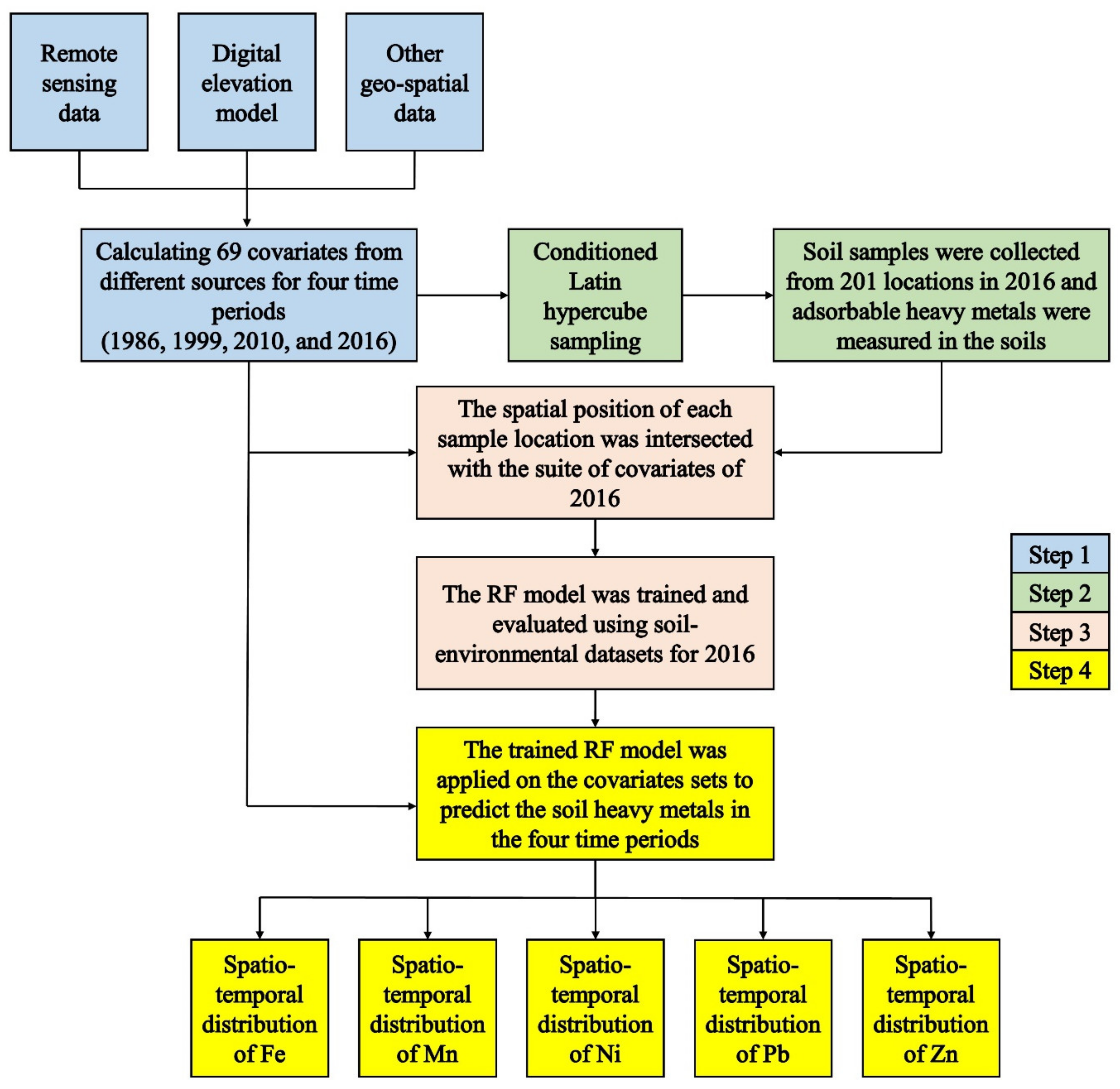
2. Materials and Methods
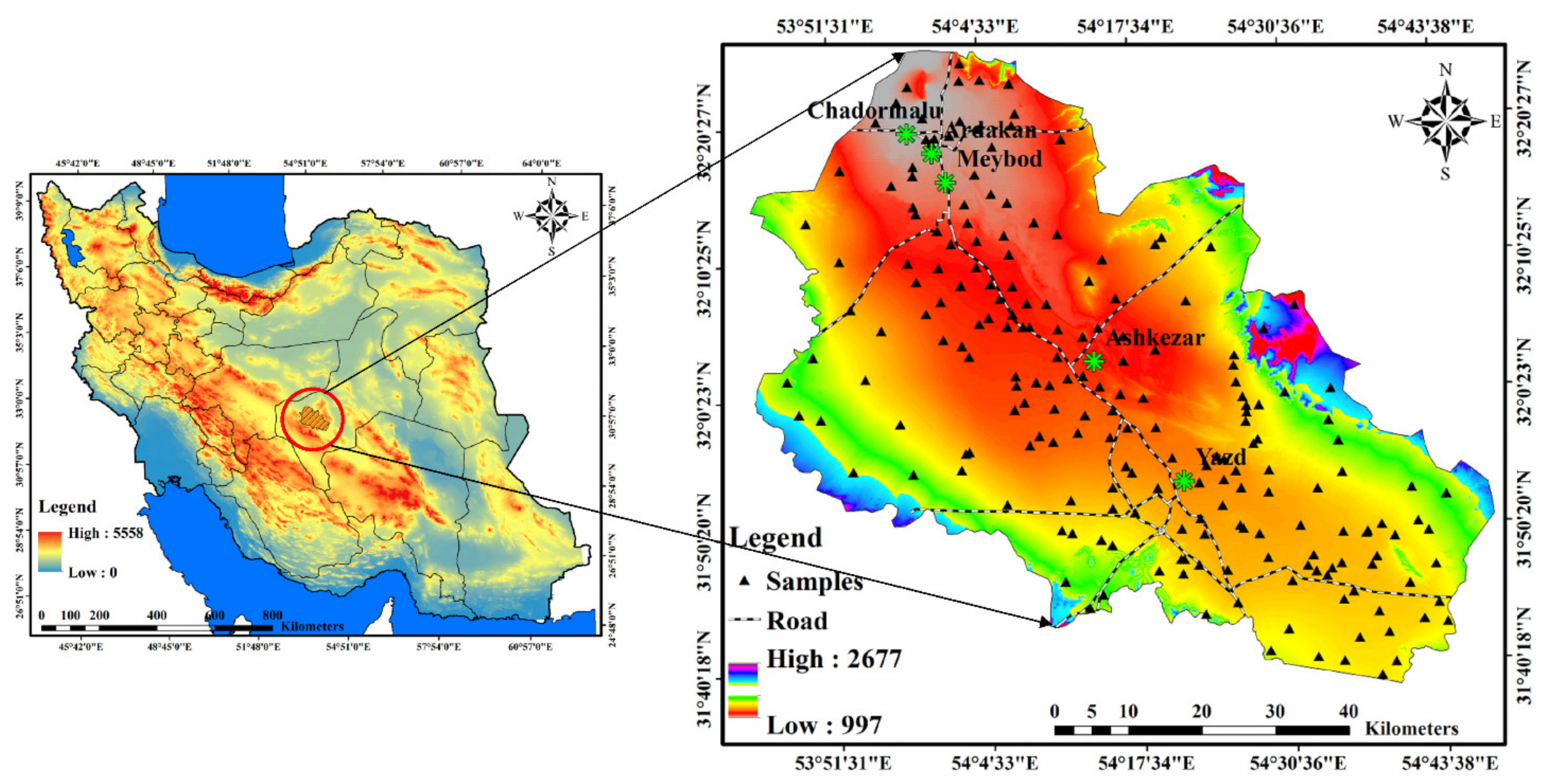
This study was conducted in four main steps (Figure 1). In Step 1, a wide range of environmental covariates was obtained from various sources and was calculated for four time periods (1986, 1999, 2010, and 2016). In Step 2, the 201 sample locations were identified within the study area using the Latin hypercube sampling (LHS) approach. Here, soil samples were collected and the adsorbable heavy metals were measured. In Step 3, the relationships between soil heavy metals and covariates were quantified using a RF model. In Step 4, the constructed RF model was applied to the covariates acquired for 1986, 1999, 2010, and 2016 to predict and map the spatial distribution of soil heavy metals for the four time periods.

2.1. Study Area

The study area is in the central plateau of Iran and has an area of 482,900 hectares. The location of the central part of the province is between 53°08′36″ and 54°85′32″E longitude and 31°21′59″ and 32°61′02″N latitude. The elevation of Yazd Province ranges from 997 to 2677 meters above mean sea level. Precipitation is low and infrequent in the region, averaging 59.2 mm per year; furthermore, evaporation rates are high, averaging 2200 to 3200 mm per year. The study area has no permanent rivers—the rivers of the plain only flow during periods of flooding (Figure 2). The population density of the region is high, with nearly 75% of the population of the Yazd Province living on the plain and working in the numerous factories and mines. Major production units of Yazd include the production of tiles and ceramics, and this is concentrated along the Ardakan-Meybod-Yazd route. The ceramics industry provides more than 50% of the ceramic tiles for Iran and thus, the factories and workshops are a major source of industrial pollutants throughout the region. This region also features geological features with a vast range in age, from the oldest (Precambrian) to the youngest (Holocene) (Figure 3).

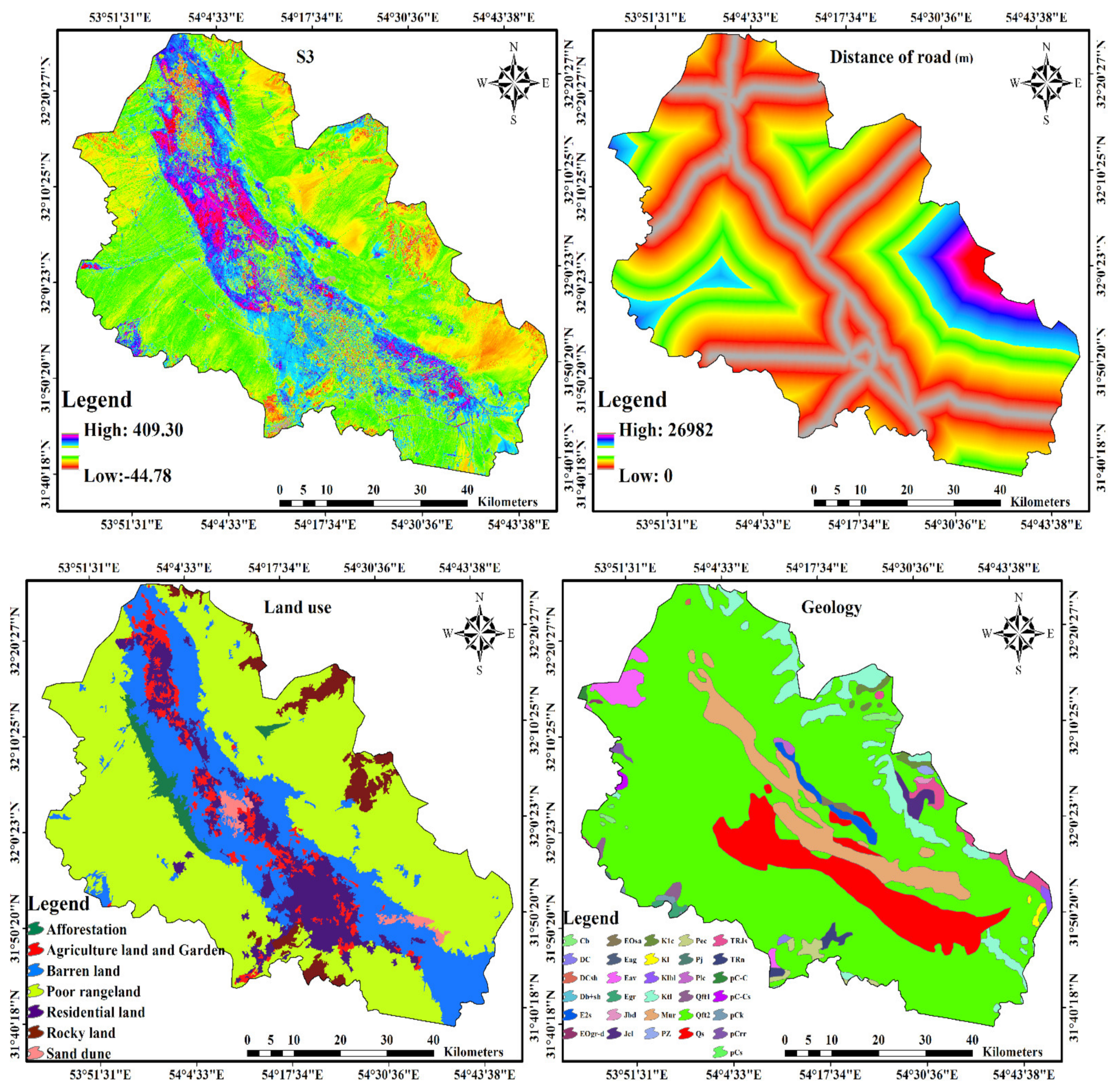
2.2. Environmental Covariates

This study used 69 environmental covariates, which were derived from DEMs, remote sensing data, land use data, geological maps, groundwater quality data, and other geospatial datasets. It should be added that all raster-based covariates were calculated for the four timesteps from 1999 to 2016. The covariates, summarized in Table A1, were resampled (aggregation or disaggregation) to a common spatial resolution of 30 m. Four examples of covariates are presented in Figure 3.

2.2.1. Digital Elevation Model

A pre-processed SRTM-derived DEM [50], with a 30 m spatial resolution, was used to derive 12 terrain attributes using SAGA GIS [51]. These attributes (e.g., slope gradient, and valley depth) are commonly used in DSM studies to represent topography (Table A2).

2.2.2. Remote Sensing Data

Landsat images were used to prepare the covariates derived from remote sensing data, which were acquired for each of the timesteps. Remote sensing data were acquired from Landsat 4 (Multispectral Scanner System; MSS) for October 7, 1986; Landsat 5 (Thematic Mapper; TM) for August 19, 1999; Landsat 7 (Enhanced Thematic Mapper Plus; ETM+), for September 3, 2010; and Landsat 8 (Operational Land Imager; OLI) for September 10, 2016. After performing geometric and radiometric corrections on the Landsat images, a total of 36 covariates were calculated. These covariates included the original Landsat bands, their principal components (PC1 to PC11), vegetative indices (e.g., normalized difference vegetation index, ratio vegetation indices), soil salinity indices, bare soil index (BI), and soil moisture indices (Table A2).

2.2.3. Land Use Map

Using the Landsat imagery described in Section 2.2.2, land use maps were developed using an object-based, controlled, classification method with seven user-defined categories (afforested, agricultural land and garden, barren land, poor rangeland, residential land, rocky land, and sand dune) [52] (Table A2).

2.2.4. Geological Map

Geological information was obtained through field operations, a review of case reports, and the integration of geological maps. Studies show that the area has rocks and sediments from both the oldest (Precambrian) and youngest (Holocene) geological organizations. The Precambrian formations consist of various types of metamorphic rocks, as well as igneous rocks, in which even layers of gypsum can be observed (Table A2).

2.2.5. Groundwater Quality Parameters

To investigate the quality of groundwater samples and their potential effect on the heavy metal concentrations in the soil, data were acquired from 103 wells from a 1986–2016 water monitoring survey. The well water data included measurements of several groundwater quality parameters such as bicarbonate chloride (Cl; mg L−1) and sodium (Na⁺; mg L−1) (Table A2). The inverse distance weighted (IDW) interpolation method was used to create the maps of groundwater quality parameters for the four time periods.

2.2.6. Other Geospatial Data

One of the main reasons for increased concentrations of heavy metals in soils can be due to rapid population growth, which affects natural resources and the environment [40]. Therefore, to investigate the effect of population change and its impact on heavy metal concentrations in soil, 10 cities (e.g., Mehriz and Yazd) were identified and a population layer was prepared. Furthermore, 478 residential points were identified in the area and the distance from these residential areas was determined. Furthermore, the distance to the nearest road and the distance to the nearest river were also included as model inputs. The major production units of the Yazd tile and ceramic industry are located along the Ardekan-Meybod-Yazd road. In the study area, 282 mines and factories were identified; hence, a layer representing the distance to the nearest mines and factories was included. To explore the effects of changes in precipitation, data from rain gauge stations located in Kharanagh, Mohammadabad, Yazd, Mahdiabadabadar, Ali Abadchehl-e Ghazi, Nir, Yazd, Meybod, Ardekanm, and Nodooshan were obtained and precipitation maps were prepared using IDW interpolation.

2.3. Soil Data and Laboratory Analysis

Topsoil samples from the 0–20 cm depth increment were collected at 201 locations using the LHS method [53] (Figure 2). Based on the understanding of the factors affecting the soil heavy metals distribution in the study area [47,52,54] and a literature review [11,13,24,26,41,55], the selected covariates (i.e., geological layers, land use, rainfall, the first eleven principal components, vegetative indices derived from remote sensing data, and Tasseled Cap differencing) were used as inputs for the Latin hypercube method. Concentrations (mg/kg−1) of Fe, Mn, Ni, Pb, and Zn were measured from an air-dried <2 mm fraction of the soil and via the nitric acid extraction method [56]. The total concentration of each element in the soil extract was determined using an Analytic Jena-novAA300 Atomic Absorption Spectrophotometer.

2.4. Random Forest

The aim of machine learning is to obtain a useful approximation of a function that is based on the relationship between input variables and the desired outputs [57]. Here, the RF model was used to find the relationship between the environmental covariates and heavy metals in the soil. The RF approach was first proposed in Breiman [58] and consists of an ensemble of individual decision trees, which may be applied for both regression and classification problems. Decision trees are a hierarchical model, which consists of a series of nodes and leaves (i.e., terminal nodes). Each node may be considered as an if-then statement, whereby the model generates a node-splitting rule that is intended to maximize the within-node homogeneity and between-node heterogeneity within the measured values. Due to the instability of an individual tree, whereby a small change in the dataset could result in a large change in the structure of decision tree, the RF learner generates a diverse set of decision trees and aggregates the models using an averaging function (when applied to regression problems). These decision trees are generated through a bootstrap sample (with replacement) of the training data and further randomness is incorporated in the model by randomly selecting a subset of covariates that are tested when establishing the splitting rules at each node. After each tree is generated, the trees are ensembled together using an averaging function. The model ensemble provides outputs that are more accurate, more stable, and less sensitive to overfitting in comparison to individual decision trees. Due to the use of bootstrap sampling, the training data that were not selected for the model (out-of-bag sample) are then used by the RF model for variable importance analysis. In this study, three main hyperparameters of the RF model were optimized, namely, ntree, mtry, and nodesize. The ntree parameter controls the number of trees within the RF; the mtry parameter controls the number of variables that are randomly selected when establishing the node-splitting rules; and the nodesize parameter controls the minimum size of the terminal nodes.
A 10-fold-cross-validation procedure was utilized to assess the performance of a RF model for predicting heavy metals. The root mean square error (RMSE), mean absolute error (MAE), coefficient of determination (R2), and the percentage of error (RMSE/average of each heavy metal) were calculated as the main validation criteria. The randomForest package in the R environment [59] was used to implement the RF model.

2.5. Historical Spatial Distributions of Soil Heavy Metals

In this study, a RF model was used to find the relationship between the environmental covariates and soil heavy metals in 2016. Then, the trained RF model for 2016 was applied to the covariates that were generated for the 1986, 1999, and 2010 periods in order to reconstruct the spatial distribution of soil heavy metals of the past [47]. The number of covariates and their spatial resolutions for the 1986, 1999, 2010, and 2016 periods were the same (Table A2).

3. Results and Discussion

3.1. Soil Data

The summary statistics for soil absorbable heavy metals are provided in Table 1. Ni had the highest coefficient of variation (1.53) while Mn had the lowest (0.75). The correlations between the absorbable heavy metals and the other soil attributes were weak but significant in some cases (Table 2). For example, Table 2 shows that Cl and EC had a positive correlation with Fe and Ni (p < 0.01); SOC had a positive correlation with Zn (p < 0.01); shear strength was positively correlated with Ni (p < 0.01) and Zn (p <0.05); bulk density had a positive correlation with Fe (p < 0.05); and HCO3 also had a positive correlation with Zn (p < 0.01).

3.2. Environmental Covariates

The covariate importance analysis of the RF model for 2016 is illustrated in Figure 4, whereby higher values of increase-in-node-purity (IncNodePurity) represent higher importance of the covariate. As can be seen, the urbanization and road construction predictors were important covariates for predicting soil heavy metals. Therefore, it can be concluded that human activities might be the main factor affecting the spatial distribution of soil heavy metals in the study area. Furthermore, it was also observed that groundwater, vegetation indices, satellite bands, and topographic attributes derived from the DEM were also important predictors. Previous studies have shown that heavy metals have strong reflectance in the visible and near-infrared regions of the electromagnetic spectrum, and their reflectance characteristics could be useful for identifying these elements [43]. Here, the red and infrared bands had high correlations with the heavy metals in the soil (Figure 4). Dana and Badea [44] showed that satellite bands, which were transformed using PCA, were an effective predictor when used for detecting contaminated farmlands. The results also confirm our original notion of the importance of human activities on the distribution of heavy metal concentrations; for example, the concentration of Pb was higher in soils that were in close proximity to roads. Similarly, Karrari et al. [40] reported higher Pb contamination of soils in the vicinity of polluted and industrialized cities in Iran. This also was aligned with the findings of Kheir et al. [60], who showed the influence of roads as being the third most important factor affecting heavy metal accumulation in the soils after urban margins and waste disposal areas.

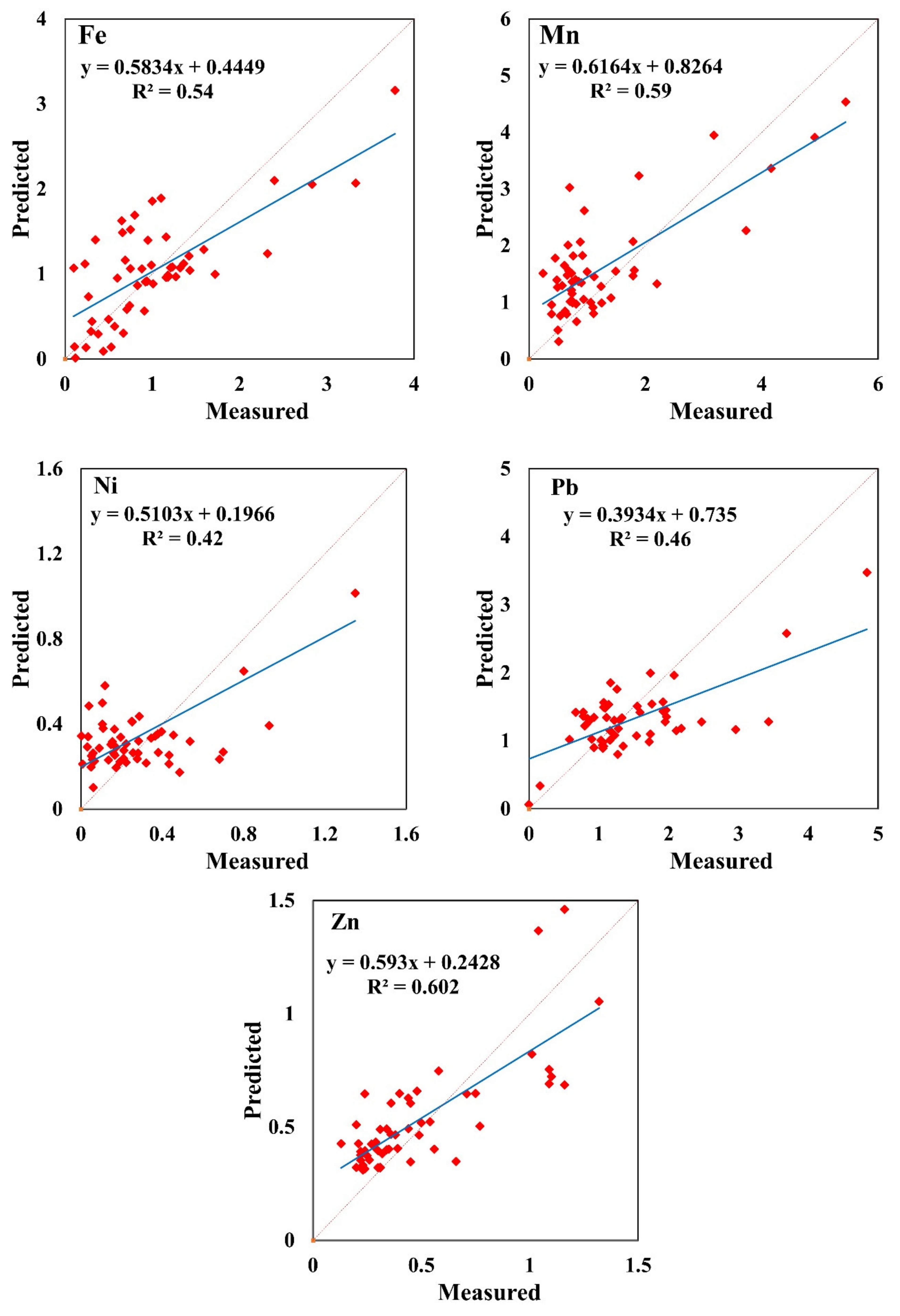
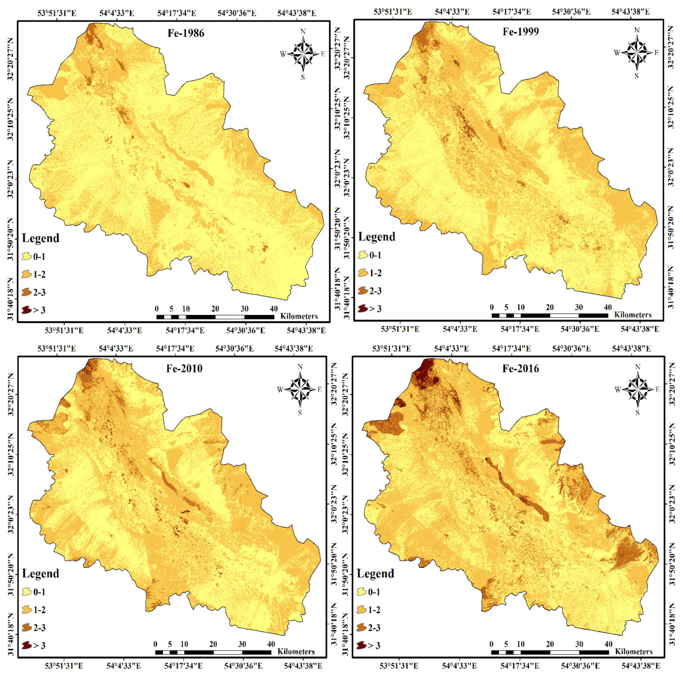
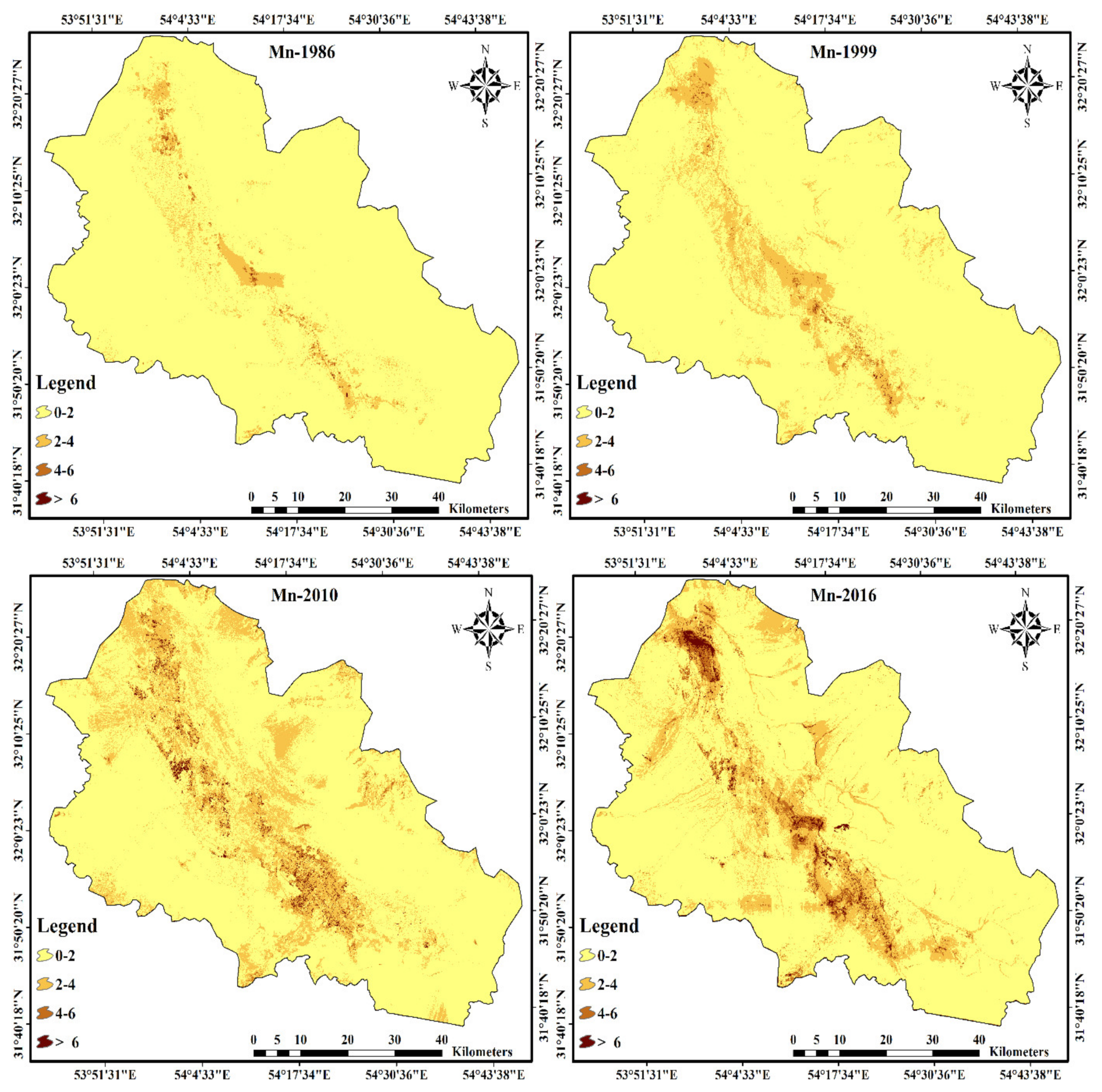
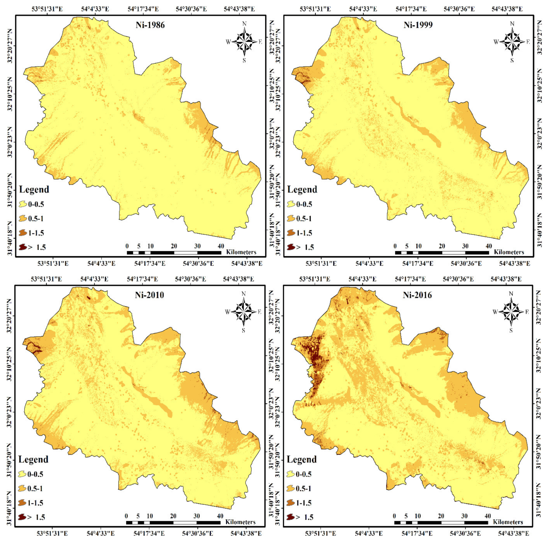
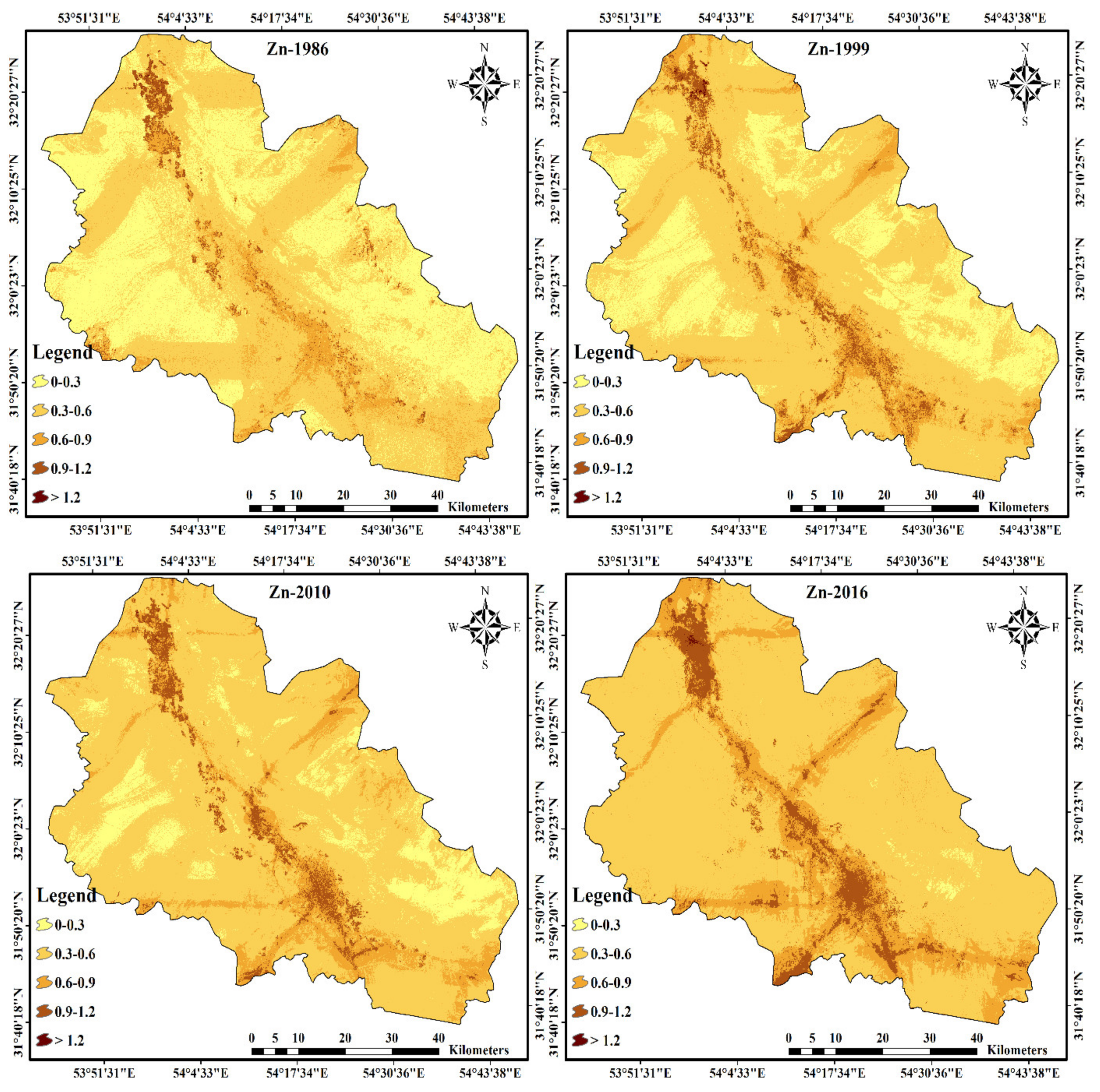
3.3. Current Distributions of Heavy Metals (2016)

Upon optimizing the RF model parameters for 2016, the model was validated using the MAE, RMSE, R2, and %Error metrics, which were calculated based on the actual and the predicted heavy metal values for the soil (Table 3). The validation results indicated that the RF models performed reasonably well in terms of the MAE, RMSE, R2, and %Error metrics, with values ranging from 0.11 to 0.47, 0.15 to 0.60, 0.41 to 0.60, and 25 to 50, respectively. The effectiveness of the RF models was further confirmed in Figure 5, which shows a moderate correlation between the measured and predicted heavy metal concentrations. It should be highlighted that R2 values > 70% are uncommon and values of R2 < 50% are common in DSM studies [54,61,62]. The %Error values in Table 3 indicated that the RF model had the highest accuracy in predicting Pb, sequentially followed by Zn, Mn, Fe, and Ni. Similar to the results of this study, Amirian-Chakan et al. [36], Nabiollahi et al. [63], and Taghizadeh-Mehrjardi et al. [45] also used the RF model for predicting different soil properties in various regions of Iran and reported acceptable levels of accuracy (Table S1).

3.4. Historical Distributions of Heavy Metals (1986, 1999, and 2010)

Comparing the results of total concentrations of heavy metal distributions with the quality standards for soil resources in Iran, it was observed that the average concentration of heavy metals in the study area was lower than the standards. Using the environmental datasets that represented the historical conditions, the 2016 RF model was used to estimate the heavy metal concentrations for 1986, 1999, and 2010. As a result, the heavy metal maps of the soil were classified according to their conditions and their composition in the study area. Figure 6, Figure 7, Figure 8, Figure 9 and Figure 10 show the maps of estimated heavy metal distribution in soils of the Yazd-Ardekan plain for 1986, 1999, and 2010. These findings suggest that some of the spatial variation of these heavy metals is partially due to factors such as mining operations, extraction, and activities. This further suggests that the industrial materials and smoke caused by the passing service vehicles and vehicles on the adjacent highway and Bandar Abbas-Tehran road should be controlled. Although the point sources of pollution are intuitively linked to the spatial distribution of heavy metals, other factors such as wind speed and direction are also important factors and should therefore not be neglected.

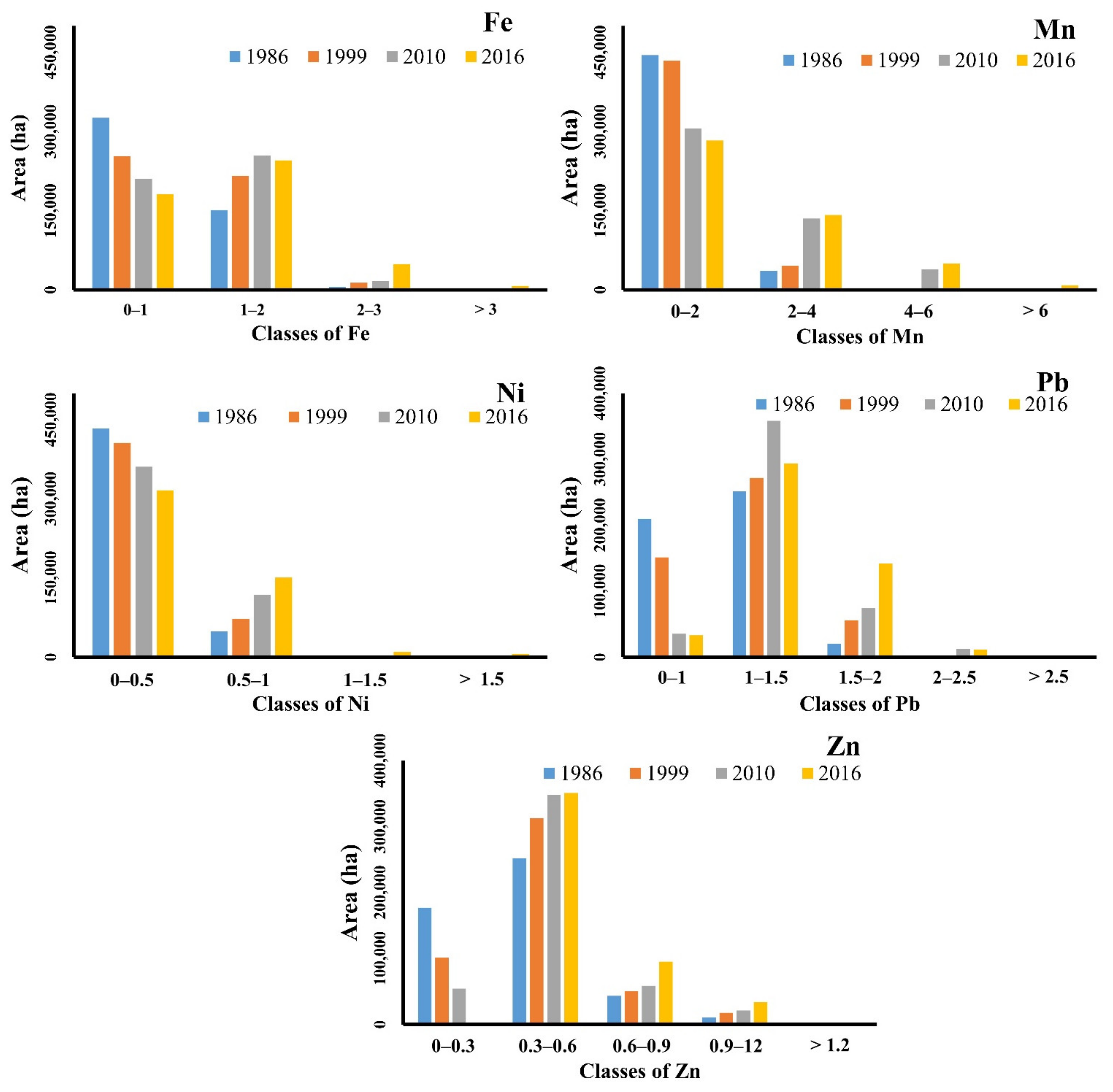
3.5. Comparison of Heavy Metal Distributions (1986 to 2016)

After the maps of soil heavy metals were prepared for each time step, the areal extent of each class for every heavy metal was calculated and presented in Figure 11. According to Figure 11, the change in Fe levels in the area between 1986 and 2016 showed that the area of the 0–1 mg/kg−1 class decreased by 144,683 ha and the areas of the 1–2, 2–3, and >3 mg/kg−1 classes increased by 94,169 ha, 43,023 ha, and 7,491 ha, respectively. Between 1986 and 2016 (Figure 6 and Figure 11), the greatest percentage of Fe in the 0–1 mg/kg−1 class was in 1986, while the areal extent of the class >3 mg/kg−1 was very small. In 2016, however, the areal of extent of the 0–1 mg/kg−1 class decreased by more than 30% and the areal extent of the 1–2 mg/kg−1 increased by more than 19.5%, indicating an overall increase in Fe concentrations for the region.
There were also substantial increases in Mn concentrations where the 2–4, 4–6, and >6 mg/kg−1 classes increased by 22% (106,090 ha), 9.80% (47,339 ha), and 1.76% (8519 ha), respectively; in comparison, the areal extent of the 0–2 mg/kg−1 class decreased by 33.53% (161,948 ha) between 1986 and 2016 (Figure 11). Mn concentrations in the Yazd-Ardekan plain have historically increased from 1986 to 2016 due to mining activities and factories. According to the statistics from the Yazd Province Mining Industry Organization, by 2017, there were 566 active mines in Yazd. According to the Mn map (Figure 7 and Figure 11), there were moderate (2–4 mg/kg−1) concentrations across the whole region and these concentrations need to be managed. Although the main source of naturally occurring Mn in the soil is from the Earth’s crust, the anthropogenic sources of contamination are linked to urban wastewater discharge, sewage sludge, combustion of fossil fuels, mines, and factories [64].
Similar spatio-temporal changes were observed for Ni concentrations whereby the areal extent of the 0.5–1, 1–1.5, and >1.5 mg/kg−1 classes for Ni between 1986 and 2016 increased by 21.18% (102,317 ha), 1.18% (8786 ha), and 1.20% (5805 ha), respectively, while the areal extent of the 0–0.5 mg/kg−1 class decreased by 24.20% (116,908 ha). Overall, the highest Ni concentrations were found in pastures where the soil quality is low (Figure 8 and Figure 11). Contrary to expectations, the location of mines and factories, agricultural lands, gardens, and residential lands had little influence on Ni concentrations, indicating that the element is not related to land use. Studies such as Mico et al. [2] have shown that the Ni concentrations in the soil are related to parent materials in the Mediterranean region. Based on Figure 8 and the land use map (Figure 3), the amount of Ni seems to have little to do with land use.
With respect to Pb concentrations, the areal extent of the 1–1.5, 1.5–2, and >2.5 mg/kg−1 classes increased by 8.75% (42,258 ha), 25.18% (121,633 ha), and 2.18% (10,562 ha), respectively, while the areal extent of the 0–1 mg/kg−1 class decreased by 36.56% (176,565 ha) (Figure 11). Furthermore, the Pb concentration maps indicated that the distribution of Pb was focused at the center to the southern and western regions of the study area (shown in dark brown—Figure 9 and Figure 11). In these areas, high concentrations of Pb were due to its accumulation from mines, factories, agricultural lands, gardens, and residential lands. The reason for this may be the tendency of this element to accumulate in smaller soil particles (clay and silt) [65]. Our results were in accordance with the findings of Facchinelli et al. [66], who identified that the sources of Pb in the soil were controlled by human activities.
Lastly, the distribution of Zn concentrations increased for the 0.3–0.6, 0.6–0.9, 0.9–1.2, and >1.2 mg/kg−1 classes by 20.49% (98,963 ha), 10.70% (51,716 ha), 4.87% (23,524 ha), and 0.10% (454 ha), while the areal extent of the 0–0.3 mg/kg−1 class decreased by 36.16% (174,657 ha; Figure 11). Furthermore, the predicted maps indicated that in the areas where mines, factories, and roads were located, there was a corresponding accumulation of Zn that was moderately high (Figure 10 and Figure 11). In a study on surface soils in Spain [23], human activities and the type of parent materials were linked to increased Zn concentrations in the agricultural soils of the region. Similar findings were shown in Chen et al. [41], where there were also links between Zn concentrations, human activities, and parent materials.

4. Conclusions

It is important to recognize that the challenges related to heavy metal pollution of soil are a by-product of development and industrialization efforts and are therefore difficult to address. There is a need for continuous modeling and monitoring of potentially contaminated areas. This study integrates geochemical analysis, remote sensing data, and predictive modeling as basic steps in monitoring the soils of heavily contaminated areas. Soil monitoring is necessary to identify possible contamination sources and appropriate corrective and remedial actions; and sustainable land use management practices in relation to mining, agriculture, and urban development. Here, the RF model was applied for the spatio-temporal prediction of Fe, Mn, Ni, Pb, and Zn concentrations in the central arid region of Iran. The overall trends indicated that the concentration and spatial distribution of these heavy metals have historically increased from 1986 to 2016. This study provides fundamental knowledge on heavy metal contamination in soils and will facilitate decision making practices, support soil remedial practices for contaminated areas, and assist in targeted conservations measures.

Supplementary Materials

The following are available online at https://www.mdpi.com/article/10.3390/rs13091698/s1, Table S1: Validation results for soil heavy metal concentrations predicted using machine learning models.

Author Contributions

Conceptualization, H.F. and R.T.-M.; methodology, R.T.-M. and H.F.; software, R.T.-M. and H.F.; validation, H.F., M.A.H.A., H.S., R.K. and T.S.; formal analysis, H.S., R.T.-M. and M.A.H.A.; investigation, H.F., M.A.H.A., H.S. and R.T.-M.; resources, H.F.; data curation, H.F., M.A.H.A., H.S., R.K., B.H. and T.S.; writing—original draft preparation, H.F., M.A.H.A., H.S., R.K., B.H. and T.S.; writing—review and editing, H.F., M.A.H.A., H.S., R.K., B.H. and T.S.; visualization, R.T.-M.; supervision, M.A.H.A. and R.T.-M. All authors have read and agreed to the published version of the manuscript.

Funding

This study is financially supported by the Yazd University. The work of Ruhollah Taghizadeh-Mehrjardi has been supported by the Alexander von Humboldt Foundation under the grant number: Ref 3.4-1164573-IRN-GFHERMES-P. Ruhollah Taghizadeh-Mehrjardi and Thomas Scholten thanks the German Research Foundation (DFG) for supporting this research through the Collaborative Research Center (SFB 1070) ‘Resource Cultures’ (subprojects Z, S and B02) and the DFG Cluster of Excellence ‘Machine Learning—New Perspectives for Science’, EXC 2064/1, project number 390727645. We acknowledge support by the Open Access Publishing Fund of University of Tübingen.

Informed Consent Statement

Not applicable.

Data Availability Statement

The data presented in this study are available on request from the corresponding author. The data are not publicly available due to privacy restrictions.

Conflicts of Interest

The authors declare no conflict of interest.

Appendix A

Table A1. A list of environmental covariates used to predict soil heavy metals.
CovariatesDefinitionReferenceResolution
Analytical hillshadeAngle between the surface and the incoming light beams [51] 30 m
Mass balance indexBalance between soil mass deposited and eroded [51]30 m
Vertical distance to channel network (m)Calculates the vertical distance to a channel network base level [51]30 m
Diurnal anisotropic heatingCalculates a simple approximation of the anisotropic diurnal heat [51]30 m
Flow accumulation (number of cells)Calculates accumulated flow [51]30 m
Effective air flow heights (m)Calculates effective air flow heights [51]30 m
Slope gradient (degree)Average gradient above flow path [51]30 m
Valley depth (m)Relative position of the valley [51]30 m
Terrain ruggedness indexMeasures terrain ruggedness [51]30 m
Average view distanceLand-surface parameters specific to topo-climatology [51]30 m
Wind effectDimensionless index indicating areas exposed to wind [51]30 m
Wind expositionDimensionless index highlighting wind-exposed pixels [51]30 m
Difference vegetation index (DVI)NIR −Red [67]30 m
Enhanced vegetation index (EVI)G × (NIR − Red)/(NIR + c1 × Red − c2 × Blue + L) [67]30 m
Global vegetation index (GVI)−0.29⋅ (G) −0.56 (Red) + 0.6 (IR) + 0.49 (ΝΙR) [67]30 m
Infrared percentage vegetation index (IPVI)NIR/(NIR + Red) [68]30 m
Normalized difference vegetation index (NDVI)(Red − NIR)/(Red + NIR) [69]30 m
Blue (0.45–0.515 μm)Reflectance value of Landsat satellite band Landsat satellite 30 m
Green (0.525–0.605 μm)Reflectance value of Landsat satellite band Landsat satellite 30 m
Red (0.63–0.69 μm)Reflectance value of Landsat satellite band Landsat satellite 30 m
Near infrared (0.75–0.90 μm)Reflectance value of Landsat satellite band Landsat satellite 30 m
Shortwave infrared (1.55–1.75 μm)Reflectance value of Landsat satellite band Landsat satellite 30 m
Principal components of Landsat bandsPC1, PC2, PC3, and PC4 [70]30 m
Normalized-NDVI(NIR − (TM1 + Green))/(NIR + (TM1 + Green)) [69]30 m
Optimized soil-adjusted vegetation index (OSAVI)(NIR −Red)/(NIR + Red + 0.16) [71]30 m
PD 311Red − TM1 [72]30 m
PD 312(Red − Blue)/(Red + TM1) [72]30 m
PD 321Red − Green [72]30 m
PD 322(Red − Green)/(Red + Green) [72]30 m
Ratio-basedNIR/(Blue + Green) [69]30 m
Ratio vegetation index (RVI)(NIR/Red) [73]30 m
Soil-adjusted vegetation index (SAVI)((NIR − Red)/(NIR + Red + L)) × (1 + L) [67]30 m
Stress-related(TM1 × Green)/Red [69]30 m
Transformed vegetation index (TVI)(SWIR − Red)/(SWIR + Red) [74]30 m
VIT01Red/Thermal [75]30 m
VTI02Thermal/(Red + SWIR) [75]30 m
VIT03Thermal/Red [75]30 m
VIT04Thermal/(SWIR + Green) [75]30 m
Brightness indexBI = ((Red × Red) + (NIR × NIR))^0.5[76]30 m
Normalized difference moisture index (NDMI)NDMI = (NIR − SWIR)/(NIR + SWIR) [77]30 m
Normalized difference snow index (NDSI)NDSI = (Red − NIR)/(Red + NIR) [78]30 m
Salinity index1 (S1)S1 = Blue/Red [79]30 m
Salinity index2 (S2)S2 = (Blue − Red)/(Blue + Red) [79]30 m
Salinity index3 (S3)S3 = (Green × Red)/Blue [79]30 m
Salinity index4 (S4)S4 = (Blue × Red)/Green [79]30 m
Salinity index5 (S5)S5 = (Red × NIR)/Green [79]30 m
Salinity index6 (S6)S6 = (Blue × Red)^0.5[79]30 m
Salinity index7 (S7)S7 = (Green × Red)^0.5[79]30 m
Salinity index8 (S8)S8 = ((Blue)2 × (Green)2 × (Red)2)^0.5[79]30 m
Land use mapRepresenting the uses of a "unit" of land Landsat satellite 30 m
Distance from mines (m)Euclidean distance to mines areas [80]30 m
Distance from urban (m)Euclidean distance to urban areas [80]30 m
Distance from population (m)Euclidean distance to population centers [80]30 m
Distance from river (m)Euclidean distance to the rivers [80]30 m
Distance from road (m)Euclidean distance to the roads [80]30 m
Geology mapRepresenting the various geological features [47]30 m
Groundwater quality parametersHCO3, Cl, SO4 2−, Na+, Ca2+, Mg2+, EC, TH, SAR, and TDS[47]30 m
Table A2. Definition of geology map units.
UnitDefinitionArea (ha)
Db+sh-32.4
DC-340.5
DCshAlternation of shale, marl, and limestone126.5
E2sSandstone, marl, and limestone3823.9
Eag-14.4
CbAlternation of dolomite, limestone, and verigated shale1632.6
Egr-918.2
EOgr-d-167.1
EOsaSalt dome785.1
Eav-6445.5
pC-CLate proterozoic–early Cambrian undifferentiated rocks361.6
JbdDark grey, well-bedded, oolitic, ammonitiferous limestone, sandstone, and shale 358.2
Jel-2583.6
TRJsSandstone, siltstone, and claystone, variously alternating with thin coal seams 4779.9
KlblGrey, thick-bedded to massive oolitic limestone709.4
K1cSandstone and conglomerate2283.3
KtlThin to meddium-bedded argillaceous limestone and thick-bedded to massive, grey orbitolina bearing limestone 24,338.9
KlLower Cretaceous undifferentiated rocks651.8
PZUndifferentiated Paleozoic rocks477.6
PecConglomerate and sandstone2395.2
pCkDull green grey slaty shales with subordinate intercalation of quartzitic sandstone 661.0
pCrrMeta-ryolite574.6
pC-CsThick dolomite and limestone unit, partly cherty with thick shale intercalations 533.9
pCs-69.8
PjMassive to thick-bedded, dark-gray, partly reef type limestone and a thick yellow dolomite band in the upper part 94.2
PlcPolymictic conglomerate and sandstone649.4
QsUnconsoliated wind-blown sand deposits and back shore sand dunes45,525.9
Qft1High level piedmont fan and valley terraces deposits1197.6
Qft2Low level piedmont fan and valley terraces deposits347,704.3
TRnGreenish gray shale and gray limestone1844.9
MurRed marl, gypsiferous marl, sandstone, and conglomerate 30,819.1

References

  1. Lin, Y.P. Multivariate geostatistical methods to identify and map spatial variations of soil heavy metals. Environ. Geol. 2002, 42, 1–10. [Google Scholar] [CrossRef]
  2. Micó, C.; Recatalá, L.; Peris, M.; Sánchez, J. Assessing heavy metal sources in agricultural soils of an European Mediterranean area by multivariate analysis. Chemosphere 2006, 65, 863–872. [Google Scholar] [CrossRef] [PubMed]
  3. He, J.; Yang, Y.; Christakos, G.; Liu, Y.; Yang, X. Assessment of soil heavy metal pollution using stochastic site indicators. Geoderma 2019, 337. [Google Scholar] [CrossRef]
  4. Li, Z.; Ma, Z.; van der Kuijp, T.J.; Yuan, Z.; Huang, L. A review of soil heavy metal pollution from mines in China: Pollution and health risk assessment. Sci. Total Environ. 2014, 468–469, 843–853. [Google Scholar] [CrossRef]
  5. Tan, K.; Ma, W.; Chen, L.; Wang, H.; Du, Q.; Du, P.; Yan, B.; Liu, R.; Li, H. Estimating the distribution trend of soil heavy metals in mining area from HyMap airborne hyperspectral imagery based on ensemble learning. J. Hazard. Mater. 2021, 401, 123288. [Google Scholar] [CrossRef] [PubMed]
  6. Shi, T.; Guo, L.; Chen, Y.; Wang, W.; Shi, Z.; Li, Q.; Wu, G. Proximal and remote sensing techniques for mapping of soil contamination with heavy metals. Appl. Spectrosc. Rev. 2018, 53, 783–805. [Google Scholar] [CrossRef]
  7. Al-Khashman, O.A. Heavy metal distribution in dust, street dust and soils from the work place in Karak Industrial Estate, Jordan. Atmos. Environ. 2004, 38, 6803–6812. [Google Scholar] [CrossRef]
  8. Subida, M.D.; Berihuete, A.; Drake, P.; Blasco, J. Multivariate methods and artificial neural networks in the assessment of the response of infaunal assemblages to sediment metal contamination and organic enrichment. Sci. Total Environ. 2013, 450–451, 289–300. [Google Scholar] [CrossRef] [Green Version]
  9. Fu, F.; Wang, Q. Removal of heavy metal ions from wastewaters: A review. J. Environ. Manag. 2011, 92, 407–418. [Google Scholar] [CrossRef]
  10. Wang, D.; He, Y.; Liang, J.; Liu, P.; Zhuang, P. Distribution and source analysis of aluminum in rivers near Xi’an City, China. Environ. Monit. Assess. 2013, 185, 1041–1053. [Google Scholar] [CrossRef] [PubMed]
  11. Yang, Q.; Li, Z.; Lu, X.; Duan, Q.; Huang, L.; Bi, J. A review of soil heavy metal pollution from industrial and agricultural regions in China: Pollution and risk assessment. Sci. Total Environ. 2018, 642, 690–700. [Google Scholar] [CrossRef] [PubMed]
  12. Keller, A.; von Steiger, B.; van der Zee, S.E.A.T.M.; Schulin, R. A Stochastic Empirical Model for Regional Heavy-Metal Balances in Agroecosystems. J. Environ. Qual. 2001, 30, 1976–1989. [Google Scholar] [CrossRef] [PubMed]
  13. Keller, A.; Schulin, R. Modelling regional-scale mass balances of phosphorus, cadmium and zinc fluxes on arable and dairy farms. Eur. J. Agron. 2003, 20, 181–198. [Google Scholar] [CrossRef]
  14. Tan, M.Z.; Xu, F.M.; Chen, J.; Zhang, X.L.; Chen, J.Z. Spatial Prediction of Heavy Metal Pollution for Soils in Peri-Urban Beijing, China Based on Fuzzy Set Theory1 1 Project supported by the National Natural Science Foundation of China (Nos. 40571065 and 40235054) and the National Key Basic Research Support. Pedosphere 2006, 16, 545–554. [Google Scholar] [CrossRef]
  15. Wang, H.; Yilihamu, Q.; Yuan, M.; Bai, H.; Xu, H.; Wu, J. Prediction models of soil heavy metal(loid)s concentration for agricultural land in Dongli: A comparison of regression and random forest. Ecol. Indic. 2020, 119. [Google Scholar] [CrossRef]
  16. Cao, W.; Zhang, C. A Collaborative Compound Neural Network Model for Soil Heavy Metal Content Prediction. IEEE Access 2020, 8, 129497–129509. [Google Scholar] [CrossRef]
  17. Zhao, Y.F.; Shi, X.Z.; Huang, B.; Yu, D.S.; Wang, H.J.; Sun, W.X.; Öboern, I.; Blombäck, K. Spatial Distribution of Heavy Metals in Agricultural Soils of an Industry-Based Peri-Urban Area in Wuxi, China1 1 Project supported by the RURBIFARM (Sustainable Farming at the Rural-Urban Interface) project of the European Union (No. ICA4-CT-2002-10021). Pedosphere 2007, 17, 44–51. [Google Scholar] [CrossRef]
  18. Cao, J.; Li, C.; Wu, Q.; Qiao, J. Improved Mapping of Soil Heavy Metals Using a Vis-NIR Spectroscopy Index in an Agricultural Area of Eastern China. IEEE Access 2020, 8, 42584–42594. [Google Scholar] [CrossRef]
  19. Adimalla, N.; Chen, J.; Qian, H. Spatial characteristics of heavy metal contamination and potential human health risk assessment of urban soils: A case study from an urban region of South India. Ecotoxicol. Environ. Saf. 2020, 194, 110406. [Google Scholar] [CrossRef] [PubMed]
  20. Li, M.; Shao, Q. An improved statistical approach to merge satellite rainfall estimates and raingauge data. J. Hydrol. 2010, 385, 51–64. [Google Scholar] [CrossRef]
  21. Li, X.; Feng, L. Multivariate and geostatistical analyzes of metals in urban soil of Weinan industrial areas, Northwest of China. Atmos. Environ. 2012, 47, 58–65. [Google Scholar] [CrossRef]
  22. He, M.; Yan, P.; Yu, H.; Yang, S.; Xu, J.; Liu, X. Spatiotemporal modeling of soil heavy metals and early warnings from scenarios-based prediction. Chemosphere 2020, 255, 126908. [Google Scholar] [CrossRef] [PubMed]
  23. Rodríguez Martín, J.A.; Arias, M.L.; Grau Corbí, J.M. Heavy metals contents in agricultural topsoils in the Ebro basin (Spain). Application of the multivariate geoestatistical methods to study spatial variations. Environ. Pollut. 2006, 144, 1001–1012. [Google Scholar] [CrossRef]
  24. McGrath, D.; Zhang, C.; Carton, O.T. Geostatistical analyses and hazard assessment on soil lead in Silvermines area, Ireland. Environ. Pollut. 2004, 127, 239–248. [Google Scholar] [CrossRef] [PubMed]
  25. Hu, B.; Shao, S.; Ni, H.; Fu, Z.; Hu, L.; Zhou, Y.; Min, X.; She, S.; Chen, S.; Huang, M.; et al. Current status, spatial features, health risks, and potential driving factors of soil heavy metal pollution in China at province level. Environ. Pollut. 2020, 266, 114961. [Google Scholar] [CrossRef] [PubMed]
  26. Yu, A.H.; Zhao, Y. Evaluation on the soil pollution degree on two sides of highway with the fuzzy mathematics method. In Proceedings of the 2011 International Conference on Remote Sensing, Environment and Transportation Engineering, RSETE, Nanjing, China, 24–26 June 2011; pp. 4023–4026. [Google Scholar]
  27. Behrens, T.; Scholten, T. Chapter 25 A Comparison of Data-Mining Techniques in Predictive Soil Mapping. Dev. Soil Sci. 2006, 31, 353–617. [Google Scholar]
  28. Lagacherie, P. Digital soil mapping: A state of the art. In Digital Soil Mapping with Limited Data; Springer: Amsterdam, The Netherlands, 2008; pp. 3–14. ISBN 9781402085918. [Google Scholar]
  29. Veronesi, F.; Schillaci, C. Comparison between geostatistical and machine learning models as predictors of topsoil organic carbon with a focus on local uncertainty estimation. Ecol. Indic. 2019, 101, 1032–1044. [Google Scholar] [CrossRef]
  30. Lombardo, L.; Saia, S.; Schillaci, C.; Mai, P.M.; Huser, R. Modeling soil organic carbon with Quantile Regression: Dissecting predictors’ effects on carbon stocks. Geoderma 2018, 318, 148–159. [Google Scholar] [CrossRef] [Green Version]
  31. Schillaci, C.; Acutis, M.; Lombardo, L.; Lipani, A.; Fantappiè, M.; Märker, M.; Saia, S. Spatio-temporal topsoil organic carbon mapping of a semi-arid Mediterranean region: The role of land use, soil texture, topographic indices and the influence of remote sensing data to modelling. Sci. Total Environ. 2017, 601–602, 821–832. [Google Scholar] [CrossRef]
  32. Schmidt, K.; Behrens, T.; Scholten, T. Instance selection and classification tree analysis for large spatial datasets in digital soil mapping. Geoderma 2008, 146, 138–146. [Google Scholar] [CrossRef]
  33. Grimm, R.; Behrens, T.; Märker, M.; Elsenbeer, H. Soil organic carbon concentrations and stocks on Barro Colorado Island—Digital soil mapping using Random Forests analysis. Geoderma 2008, 146, 102–113. [Google Scholar] [CrossRef]
  34. Heung, B.; Ho, H.C.; Zhang, J.; Knudby, A.; Bulmer, C.E.; Schmidt, M.G. An overview and comparison of machine-learning techniques for classification purposes in digital soil mapping. Geoderma 2016, 265, 62–77. [Google Scholar] [CrossRef]
  35. Heung, B.; Hodúl, M.; Schmidt, M.G. Comparing the use of training data derived from legacy soil pits and soil survey polygons for mapping soil classes. Geoderma 2017, 290, 51–68. [Google Scholar] [CrossRef]
  36. Amirian-Chakan, A.; Minasny, B.; Taghizadeh-Mehrjardi, R.; Akbarifazli, R.; Darvishpasand, Z.; Khordehbin, S. Some practical aspects of predicting texture data in digital soil mapping. Soil Tillage Res. 2019, 194, 104289. [Google Scholar] [CrossRef]
  37. Rentschler, T.; Werban, U.; Ahner, M.; Behrens, T.; Gries, P.; Scholten, T.; Teuber, S.; Schmidt, K. 3D mapping of soil organic carbon content and soil moisture with multiple geophysical sensors and machine learning. Vadose Zone J. 2020, 19, e20062. [Google Scholar] [CrossRef]
  38. McBratney, A.B.; Mendonça Santos, M.L.; Minasny, B. On digital soil mapping. Geoderma 2003, 117, 3–52. [Google Scholar] [CrossRef]
  39. Arrouays, D.; Grundy, M.G.; Hartemink, A.E.; Hempel, J.W.; Heuvelink, G.B.M.; Hong, S.Y.; Lagacherie, P.; Lelyk, G.; McBratney, A.B.; McKenzie, N.J.; et al. GlobalSoilMap. Toward a Fine-Resolution Global Grid of Soil Properties. In Advances in Agronomy; Academic Press: Cambridge, MA, USA, 2014; Volume 125, pp. 93–134. [Google Scholar]
  40. Karrari, P.; Mehrpour, O.; Abdollahi, M. A systematic review on status of lead pollution and toxicity in Iran; Guidance for preventive measures. DARU J. Pharm. Sci. 2012, 20, 1–17. [Google Scholar] [CrossRef] [Green Version]
  41. Chen, Y.; Liu, Y.; Liu, Y.; Lin, A.; Kong, X.; Liu, D.; Li, X.; Zhang, Y.; Gao, Y.; Wang, D. Mapping of Cu and Pb contaminations in soil using combined geochemistry, topography, and remote sensing: A case study in the le’an river floodplain, China. Int. J. Environ. Res. Public Health 2012, 9, 1874–1886. [Google Scholar] [CrossRef]
  42. Shokr, M.S.; Baroudy, A.A.; El-Fullen, M.A.; El-Beshbeshy, T.R.; Ali, R.R.; Elhalim, A.; Guerra, A.J.T.; Jorge, M.C.O. Mapping of heavy metal contamination in alluvial soils of the Middle Nile Delta of Egypt. J. Environ. Eng. Landsc. Manag. 2016, 24, 218–231. [Google Scholar] [CrossRef]
  43. Choe, E.; van der Meer, F.; van Ruitenbeek, F.; van der Werff, H.; de Smeth, B.; Kim, K.W. Mapping of heavy metal pollution in stream sediments using combined geochemistry, field spectroscopy, and hyperspectral remote sensing: A case study of the Rodalquilar mining area, SE Spain. Remote Sens. Environ. 2008, 112, 3222–3233. [Google Scholar] [CrossRef]
  44. Dana, I.F.; Badea, A. Studies regarding the use of remote sensing satellite data for the identification of heavy metal pollution in agricultural fields. Ann. DAAAM 2011, 22, 1726–9679. [Google Scholar]
  45. Taghizadeh-Mehrjardi, R.; Mahdianpari, M.; Mohammadimanesh, F.; Behrens, T.; Toomanian, N.; Scholten, T.; Schmidt, K. Multi-task convolutional neural networks outperformed random forest for mapping soil particle size fractions in central Iran. Geoderma 2020, 376, 114552. [Google Scholar] [CrossRef]
  46. Fathizad, H.; Ali Hakimzadeh-Ardakani, M.; Sodaiezadeh, H.; Kerry, R.; Taghizadeh-Mehrjardi, R. Investigation of the spatial and temporal variation of soil salinity using random forests in the central desert of Iran. Geoderma 2020, 365, 114233. [Google Scholar] [CrossRef]
  47. Fathizad, H.; Ardakani, M.A.H.; Heung, B.; Sodaiezadeh, H.; Rahmani, A.; Fathabadi, A.; Scholten, T.; Taghizadeh-Mehrjardi, R. Spatio-temporal dynamic of soil quality in the central Iranian desert modeled with machine learning and digital soil assessment techniques. Ecol. Indic. 2020, 118, 106736. [Google Scholar] [CrossRef]
  48. Nabiollahi, K.; Golmohamadi, F.; Taghizadeh-Mehrjardi, R.; Kerry, R.; Davari, M. Assessing the effects of slope gradient and land use change on soil quality degradation through digital mapping of soil quality indices and soil loss rate. Geoderma 2018, 318, 16–28. [Google Scholar] [CrossRef]
  49. Mahmoudzadeh, H.; Matinfar, H.R.; Taghizadeh-Mehrjardi, R.; Kerry, R. Spatial prediction of soil organic carbon using machine learning techniques in western Iran. Geoderma Reg. 2020, 21, e00260. [Google Scholar] [CrossRef]
  50. Farr, T.G.; Kobrick, M. The Shuttle Radar Topography Mission. Rev. Geophys. 2000. [Google Scholar] [CrossRef] [Green Version]
  51. Conrad, O.; Bechtel, B.; Bock, M.; Dietrich, H.; Fischer, E.; Gerlitz, L.; Wehberg, J.; Wichmann, V.; Böhner, J. System for Automated Geoscientific Analyses (SAGA) v. 2.1.4. Geosci. Model Dev. 2015, 8, 1991–2007. [Google Scholar] [CrossRef] [Green Version]
  52. Fathizad, H.; Hakimzadeh-Ardakani, M.A.; Mehrjardi, R.T.; Sodaiezadeh, H. Evaluating desertification using remote sensing technique and object-oriented classification algorithm in the Iranian central desert. J. African Earth Sci. 2018, 145, 115–130. [Google Scholar] [CrossRef]
  53. Minasny, B.; McBratney, A.B. A conditioned Latin hypercube method for sampling in the presence of ancillary information. Comput. Geosci. 2006, 32, 1378–1388. [Google Scholar] [CrossRef]
  54. Poppiel, R.R.; Demattê, J.A.M.; Rosin, N.A.; Campos, L.R.; Tayebi, M.; Bonfatti, B.R.; Ayoubi, S.; Tajik, S.; Afshar, F.A.; Jafari, A.; et al. High resolution middle eastern soil attributes mapping via open data and cloud computing. Geoderma 2021, 385, 114890. [Google Scholar] [CrossRef]
  55. Galagan, A.O.; Korogoda, N.P.; Grodzinsky, M.D.; Obodovsky, A.G. Geoinformation modeling of soil pollution processes by lead compounds in highway geosystems. Visnyk V.N. Karazin Kharkiv Natl. Univ. Ser. Geol. Geogr. Ecol. 2020, 52, 103–118. [Google Scholar] [CrossRef]
  56. Lindsay, W.L.; Norvell, W.A. Development of a DTPA soil test for zinc, iron, manganese, and copper. Soil Sci. Soc. Am. J. 1978, 42, 421–428. [Google Scholar] [CrossRef]
  57. Hastie, R. Problems for Judgment and Decision Making. Annu. Rev. Psychol. 2001, 52, 653–683. [Google Scholar] [CrossRef] [Green Version]
  58. Breiman, L. Random forests. Mach. Learn. 2001, 45, 5–32. [Google Scholar] [CrossRef] [Green Version]
  59. Liaw, A.; Wiener, M. Classification and Regression by randomForest. R news 2002, 18–22. [Google Scholar] [CrossRef]
  60. Bou-Kheir, R.; Shomar, B.; Greve, M.B.; Greve, M.H. On the quantitative relationships between environmental parameters and heavy metals pollution in Mediterranean soils using GIS regression-trees: The case study of Lebanon. J. Geochem. Explor. 2014, 147, 250–259. [Google Scholar] [CrossRef]
  61. Taghizadeh-Mehrjardi, R.; Minasny, B.; Sarmadian, F.; Malone, B.P. Digital mapping of soil salinity in ardakan region, central iran. Geoderma 2014, 213, 15–28. [Google Scholar] [CrossRef]
  62. Taghizadeh-Mehrjardi, R.; Neupane, R.; Sood, K.; Kumar, S. Artificial bee colony feature selection algorithm combined with machine learning algorithms to predict vertical and lateral distribution of soil organic matter in South Dakota, USA. Carbon Manag. 2017, 8, 277–291. [Google Scholar] [CrossRef]
  63. Nabiollahi, K.; Eskandari, S.; Taghizadeh-Mehrjardi, R.; Kerry, R.; Triantafilis, J. Assessing soil organic carbon stocks under land-use change scenarios using random forest models. Carbon Manag. 2019, 10, 63–77. [Google Scholar] [CrossRef]
  64. Heath, P.H.; Malcolm, W.S.; Dobson, S.; World Health Organization; International Programme on Chemical Safety. Manganese and Its Compounds: Environmental Aspects; WHO: Geneva, Switzerland, 2004. [Google Scholar]
  65. Ajmone-Marsan, F.; Biasioli, M.; Kralj, T.; Grčman, H.; Davidson, C.M.; Hursthouse, A.S.; Madrid, L.; Rodrigues, S. Metals in particle-size fractions of the soils of five European cities. Environ. Pollut. 2008, 152, 73–81. [Google Scholar] [CrossRef]
  66. Facchinelli, A.; Sacchi, E.; Mallen, L. Multivariate statistical and GIS-based approach to identify heavy metal sources in soils. Environ. Pollut. 2001, 114, 313–324. [Google Scholar] [CrossRef]
  67. Huete, A.R. A soil-adjusted vegetation index (SAVI). Remote Sens. Environ. 1988, 25, 295–309. [Google Scholar] [CrossRef]
  68. Crippen, R.E. Calculating the vegetation index faster. Remote Sens. Environ. 1990, 34, 71–73. [Google Scholar] [CrossRef]
  69. Foody, G.M.; Cutler, M.E.; McMorrow, J.; Pelz, D.; Tangki, H.; Boyd, D.S.; Douglas, I. Mapping the biomass of Bornean tropical rain forest from remotely sensed data. Glob. Ecol. Biogeogr. 2001, 10, 379–387. [Google Scholar] [CrossRef]
  70. Nield, S.J.; Boettinger, J.L.; Ramsey, R.D. Digitally Mapping Gypsic and Natric Soil Areas Using Landsat ETM Data. Soil Sci. Soc. Am. J. 2007, 71, 245–252. [Google Scholar] [CrossRef] [Green Version]
  71. Rondeaux, G.; Steven, M.; Baret, F. Optimization of soil-adjusted vegetation indices. Remote Sens. Environ. 1996, 55, 95–107. [Google Scholar] [CrossRef]
  72. Arzani, H.; King, G.W. Application of Remote Sensing (Landsat TM data) for Vegetation Parameters Measurement in Western Division of NSW. In Proceedings of the International Grassland Congress, Hohhot, China, 29 June–5 July 2008. [Google Scholar]
  73. Jordan, C.F. Derivation of Leaf-Area Index from Quality of Light on the Forest Floor. Ecology 1969, 50, 663–666. [Google Scholar] [CrossRef]
  74. Pettorelli, N.; Vik, J.O.; Mysterud, A.; Gaillard, J.M.; Tucker, C.J.; Stenseth, N.C. Using the satellite-derived NDVI to assess ecological responses to environmental change. Trends Ecol. Evol. 2005, 20, 503–510. [Google Scholar] [CrossRef] [PubMed]
  75. Kullberg, E.G.; DeJonge, K.C.; Chávez, J.L. Evaluation of thermal remote sensing indices to estimate crop evapotranspiration coefficients. Agric. Water Manag. 2017, 179, 64–73. [Google Scholar] [CrossRef] [Green Version]
  76. Khan, N.M.; Rastoskuev, V.V.; Sato, Y.; Shiozawa, S. Assessment of hydrosaline land degradation by using a simple approach of remote sensing indicators. Agric. Water Manag. 2005, 77, 96–109. [Google Scholar] [CrossRef]
  77. Wilson, E.H.; Sader, S.A. Detection of forest harvest type using multiple dates of Landsat TM imagery. Remote Sens. Environ. 2002, 80, 385–396. [Google Scholar] [CrossRef]
  78. Major, D.J.; Baret, F.; Guyot, G. A ratio vegetation index adjusted for soil brightness. Int. J. Remote Sens. 1990, 11, 727–740. [Google Scholar] [CrossRef]
  79. Douaoui, A.E.K.; Nicolas, H.; Walter, C. Detecting salinity hazards within a semiarid context by means of combining soil and remote-sensing data. Geoderma 2006, 134, 217–230. [Google Scholar] [CrossRef]
  80. Danielsson, P.-E. Euclidean distance mapping. Comput. Graph. Image Process. 1980, 14, 227–248. [Google Scholar] [CrossRef] [Green Version]
Figure 1. Methodological framework for the spatio-temporal prediction of heavy metals in soils.
Remotesensing 13 01698 g001
Figure 2. Location of the study area and the distribution of sampling points with respect to elevation (m).
Remotesensing 13 01698 g002
Figure 3. Examples of covariates for the study area (for geological codes refer to Table A2).
Remotesensing 13 01698 g003
Figure 4. Covariate importance for predictions of heavy metals.
Remotesensing 13 01698 g004
Figure 5. Scatterplots of predicted and measured soil heavy metals (mg/kg−1) using the RF model.
Remotesensing 13 01698 g005
Figure 6. The spatial prediction of Fe (mg/kg−1) for 1986, 1999, 2010, and 2016.
Remotesensing 13 01698 g006
Figure 7. The spatial prediction of Mn (mg/kg−1) for 1986, 1999, 2010, and 2016.
Remotesensing 13 01698 g007
Figure 8. The spatial prediction of Ni (mg/kg−1) for 1986, 1999, 2010, and 2016.
Remotesensing 13 01698 g008
Figure 9. The spatial prediction of Pb (mg/kg−1) for 1986, 1999, 2010, and 2016.
Remotesensing 13 01698 g009
Figure 10. The spatial prediction of Zn (mg/kg−1) for 1986, 1999, 2010, and 2016.
Remotesensing 13 01698 g010
Figure 11. Bar charts showing the predicted percentage of different classes of each heavy metal for 1986, 1999, 2010, and 2016.
Remotesensing 13 01698 g011
Table 1. Descriptive statistics of soil absorbable heavy metals in the study area (mg/kg−1).
ParameterFeMnNiPbZn
Minimum0.040.000.000.000.00
Maximum6.0810.593.596.742.16
Average1.201.660.321.370.50
Standard deviation0.992.040.491.030.39
Variance0.974.180.241.050.15
Skewness2.192.654.581.731.70
CV0.780.751.531.220.82
Table 2. Pearson correlation coefficients between soil parameters and soil heavy metals.
Shear.SNaKCaMgCO3HCO3ClSOCBulk.DClaySandSiltECSAR
Fe−0.070.09−0.04−0.040.13−0.030.060.36 **0.10−0.16 *0.04−0.080.090.35 **0.04
Mn0.11−0.03−0.00−0.000.01−0.040.13−0.100.11−0.01−0.010.07−0.09−0.124−0.03
Ni−0.19 **0.130.070.07−0.02−0.03−0.010.35 **0.03−0.120.08−0.130.130.27 **0.12
Pb0.03−0.02−0.01−0.010.00−0.100.09−0.080.020.02−0.050.010.01−0.1380.06
Zn0.17 *−0.020.050.050.090.090.33 **0.050.28 **0.01−0.110.000.050.02−0.06
* Correlation is significant at the 0.05 level (2-tailed); ** correlation is significant at the 0.01 level (2-tailed); Shear.S: shear strength; Bulk.D: bulk density.
Table 3. Validation results for soil heavy metals (mg/kg−1) predicted using the RF model.
ParameterR2RMSEMAE%Error
Fe0.530.560.3746.7
Mn0.590.600.4736.1
Ni0.410.160.1150.0
Pb0.450.350.2825.5
Zn0.600.150.1030.0
Publisher’s Note: MDPI stays neutral with regard to jurisdictional claims in published maps and institutional affiliations.

