Abstract
Urban air quality mapping has been widely applied in urban planning, air pollution control and personal air pollution exposure assessment. Urban air quality maps are traditionally derived using measurements from fixed monitoring stations. Due to high cost, these stations are generally sparsely deployed in a few representative locations, leading to a highly generalized air quality map. In addition, urban air quality varies rapidly over short distances (<1 km) and is influenced by meteorological conditions, road network and traffic flow. These variations are not well represented in coarse-grained air quality maps generated by conventional fixed-site monitoring methods but have important implications for characterizing heterogeneous personal air pollution exposures and identifying localized air pollution hotspots. Therefore, fine-grained urban air quality mapping is indispensable. In this context, supplementary low-cost mobile sensors make mobile air quality monitoring a promising alternative. Using sparse air quality measurements collected by mobile sensors and various contextual factors, especially traffic flow, we propose a context-aware locally adapted deep forest (CLADF) model to infer the distribution of NO2 by 100 m and 1 h resolution for fine-grained air quality mapping. The CLADF model exploits deep forest to construct a local model for each cluster consisting of nearest neighbor measurements in contextual feature space, and considers traffic flow as an important contextual feature. Extensive validation experiments were conducted using mobile NO2 measurements collected by 17 postal vans equipped with low-cost sensors operating in Antwerp, Belgium. The experimental results demonstrate that the CLADF model achieves the lowest RMSE as well as advances in accuracy and correlation, compared with various benchmark models, including random forest, deep forest, extreme gradient boosting and support vector regression.
1. Introduction
Air pollution is regarded as the single biggest environmental threat to human health, as it causes an estimated 4.2 million deaths annually, comparable to other major global health risks, such as unhealthy diet and tobacco smoking [1]. Air pollution also has a great impact on the health-related economic activities by increasing the welfare costs associated with the incidence of disease and mortality as well as the reduction in labor productivity. In the year of 2013, the World Bank estimated that lost labor income and welfare losses due to PM2.5 exposure could reach up to USD 143 billion and USD 3.55 trillion, respectively [2]. In addition, the effect of air pollution on climate change and agricultural crops, as well as its damage to infrastructure and the environment, could lead to extra economic costs. In this context, air pollution has received widespread and long-term global attention [3,4,5,6].
Urban air quality monitoring has been carried out in the traditional way of setting up monitoring stations at fixed locations. However, due to high construction and maintenance costs, fixed monitoring stations are sparsely distributed, even in high-income countries, not to mention in low- and middle-income countries [7]. For example, there are currently only 94 regulatory NO2 monitoring stations in Belgium, a country with an area of 30,688 km2 and a population of more than 11.4 million inhabitants. On the other hand, the distribution of air pollutants can vary dramatically over short distances (<1 km) in the urban environment [8,9]. This is mainly due to the following two reasons: firstly, a large number of emission sources are unevenly distributed, such as automobile emissions; secondly, the dispersion process of air pollutants in the urban environment is extremely complex. As a result, air quality measurements obtained from the traditional fixed monitoring stations tend to be specific for that location and/or can only provide average levels for a larger area.
With the benefits of low cost, ease of use and no electricity required to operate, passive samplers have the potential to serve as an alternative to conventional active samplers in regional-scale air quality assessments [10]. Passive samplers function by chemically absorbing or physically adsorbing gaseous pollutants into the sampling medium. Currently, there are many passive samplers that are capable of providing comparable performance to active samplers [11]. However, there are some limitations of passive samplers. The sampling rate of passive samplers is affected by a variety of factors, such as sampling duration, wind speed, radiation, temperature and relative humidity. Additionally, they often require a long sampling time to obtain sufficient mass for detection, so they are not able to identify dynamic changes in air pollutants over short periods of time (<few hours).
The coarse-grained air quality maps derived from these measurements are not able to accurately capture the spatial heterogeneity and temporal variability of air pollutants, which is likely to mislead the assessment of individual exposure. Thus, in order to accurately characterize personal air pollution exposure and identify localized air pollution hotspots, there is a clear need for fine-grained air quality maps. The information provided by fine-grained air quality maps also has a variety of applications, such as assisting in establishing air quality standards, supporting improved relevant policies and helping to promote environmental equity. Given that urban air pollution changes rapidly over short distances and short periods of time, fine-grained air quality maps are valuable for providing personalized guidance to individuals. For example, an application of fine-grained air quality maps is personal travel route planning, which recommends the best time and routes for individuals (e.g., cyclists) while minimizing personal exposure to air pollution [12,13,14].
The development of low-cost sensors and Internet of Things (IoT) has turned people’s attention to mobile monitoring, a promising approach to break the limitations of coverage and spatial resolution of data collected from traditional fixed monitoring stations. Several studies have conducted mobile monitoring campaigns using a variety of mobile platforms, such as minivans [15], Street View cars [16], public buses [17,18], bicycles [19,20,21,22] and pedestrians [23,24]. Unlike these studies, we installed mobile sensors on postal vans for opportunistic mobile monitoring, which enables to improve spatial coverage by collecting large amounts of data for a long period of time at a relatively small additional cost. Nonetheless, due to the limited number of mobile sensors compared to the large measured area, the collected measurements are still too sparse in both temporal and spatial dimensions to meet the needs of fine-grained air quality maps with applications in personal air pollution exposure assessment, epidemiology, air quality management, and environmental equity. Therefore, air quality inference models need to be developed to fill the gaps.
In the last few decades, numerous methods have been developed to achieve air quality inference, including satellite remote sensing (RS) [25,26], chemical transport models (CTMs) [27,28], and land-use regression (LUR) models [29,30]. Two types of moderate resolution imaging spectroradiometer (MODIS) aerosol optical depth (AOD) data, Dark Target (DT) and Deep Blue (DB), are combined with meteorology and land use information in [25] to estimate spatial and temporal variations of PM1 concentrations in China during 2005–2014. Ref. [26] employs satellite remote-sensing to estimate long-term PM2.5 concentrations over Krasnoyarsk, Siberia, with the help of ground-based meteorological and radiosonde observations, and then calibrate the deviations in the satellite-derived PM2.5 concentrations using observations from the ground-based sensor network. The WRF-CAMx chemical transport modeling system is developed in [27] to estimate spatial concentrations of PM2.5 and PM10 for 20 Indian cities by using multi-pollutant high-resolution emissions inventory. Ref. [28] integrates observations of PM2.5 concentrations from more than 2500 stations in Europe and China during 2016–2020 with chemical transport model simulations to derive the distribution of PM2.5 at high spatiotemporal resolution. In order to measure and model street-level PM2.5 concentration in Seoul, South Korea, Ref. [29] constructs LUR models using the OpenStreetMap (OSM) geospatial data and 169 h of data, which is collected from a three-week sampling campaign across 5 routes by 10 volunteers sharing 7 low-cost air quality sensors. The seasonal and annual LUR models are developed in [30] based on 49 routine air quality monitoring stations to investigate the spatiotemporal variation of PM2.5 in Guangzhou, China. However, each of these approaches has distinct limitations. The spatial resolution of satellite remote sensing is usually between 1 km and 10 km [16], so the inferred air quality maps are coarse-grained and cannot capture the air pollution caused by local emission. Additionally, satellite remote sensing is interrupted fairly frequently and possibly for long periods of time by cloud cover [31]. CTMs are highly reliable only with the complete underlying emissions inventories, and thus they are not able to reveal unexpected emission sources. LUR models require all pollution sources to be known, which is rarely the case.
Recently, deep learning methods and machine learning methods have been introduced to try to solve some of these problems. A support vector machine (SVM) model is constructed in [32] with an air quality monitoring network using the radial basis function kernel, and its capability to forecast ground-level PM2.5 in a populated city with complex topography has been validated in Bogota, Colombia. Ref. [33] captures the non-linear relationship between the NO2 concentrations and predictors using random forest and develops a spatiotemporal land use random forest (LURF) model to obtain accurate NO2 estimates for prenatal exposure assessments in a metropolitan area of Japan. The extreme gradient boosting (XGBoost) algorithm has been proven to be an effective and advanced machine learning approach for urban air pollution monitoring using large amounts of mobile sensor data in [34]. The AVGAE algorithm we proposed in [35,36] treats the air quality inference problem as a matrix completion problem on graphs using the road-network topology and the incomplete discretized measurements, and then addresses this problem with a novel deep learning solution based on variational graph auto-encoders. However, deep learning methods have common limitations, such as relying on expensive GPUs to support the computation and poor explainability. The GCRF algorithm we proposed previously [37] captures the correlation between air pollution and various contextual features through a series of random forest (RF) models. In addition to the global RF model, it also constructs a local RF model for each measurement by considering the K-nearest neighbors in both geographical and feature space, which improves the accuracy but increases the computational cost. Moreover, neither of these models take into account traffic flow as an essential contextual feature.
Another important aspect that needs to be considered in air quality inference models is the variety of contextual factors that have important impacts on the spatiotemporal distribution of air pollutants in urban environments. The most frequently mentioned factors include meteorology, traffic flow and transportation network. The dispersion and development of air contaminants are closely connected with meteorological features, such as temperature, humidity, wind speed and wind direction [38,39,40]. Automobile emissions along roadways, especially from older diesel engines, have been shown to be the leading and direct source of traffic-related air pollution [41]. In addition, the local effect of traffic flow on roads causes air pollutant concentration to fluctuate over short periods of time and over short distances. Urban expressways and main roads carry much more traffic volume than local secondary roads, and hence the road type also takes a crucial role in measuring traffic-related air pollutants. Other features of the transportation network, including road length, road area, and number of major intersections, have been discovered to be applicable by several studies [42,43,44].
In this study, we address these challenges of fine-grained urban air quality mapping by exploring the potential of combining air quality data collected from mobile monitoring with diverse contextual factors into a data-driven machine learning model. The mobile monitoring campaign was conducted by 17 postal vans equipped with low-cost air quality sensors and GPS devices in Antwerp, Belgium. Mobile platforms allow sensors to take measurements at different locations in the city, significantly increasing the coverage of sensing area without the constraints and additional costs of installing sensors at fixed locations.
Using these data and contextual factors, including meteorological information, road type and traffic flow, we propose a context-aware locally adapted deep forest (CLADF) model for air quality inference as an improved and extended version of our previously proposed GCRF model [37]. The CLADF model exploits deep forests to construct a local model for each cluster, composed of measurements that share similar contextual features. In particular, traffic flow is adopted as an important contextual feature. The CLADF model improves accuracy, reduces redundancy and saves computational costs compared to the GCRF model.
The experimental results in Section 3.1 demonstrate that the CLADF model has enhanced performance with the metrics, such as root mean square error (RMSE), mean absolute error (MAE), index of agreement (IA), accuracy and correlation coefficient (r) compared to different baseline models, including random forest (RF), deep forest (DF), extreme gradient boosting (XGBoost) and support vector regression (SVR). Our previous work demonstrates the potential and feasibility of mobile air pollution monitoring using low-cost sensors and contributes to the emerging field of combining mobile monitoring and machine learning techniques. Our work in this paper illustrates the superiority of the proposed CLADF model through extensive and diverse validation experiments. Overall, our main contributions can be summarized as follows:
- We develop a general approach to integrate various contextual features and aggregate sparse mobile air quality measurements into our air quality inference model for fine-grained urban air quality mapping.
- We utilize three different types of contextual features, including meteorology, road network and traffic flow to characterize the spatiotemporal distribution of NO2.
- We propose a novel air quality inference model called CLADF, which introduces deep forests to build context-aware local models, to generate a fine-grained air quality map.
- We demonstrate through evaluation experiments on a real-world data set that the CLADF model has superior performance in comparison with different baseline models, including RF, DF, XGBoost and SVR.
The remainder of this paper is organized as follows: Section 2 describes the various datasets used in this study, including air quality data and different contextual factors, as well as the proposed algorithm for air quality inference. Section 3 provides the experimental results, and Section 4 draws conclusions and possible extensions.
2. Materials and Methods
In this section, we first describe the opportunistic mobile monitoring campaign conducted in the city of Antwerp and the air quality dataset collected to be used in this study. Next, we explain the methods and procedures of air quality data processing and aggregation. Then, we present the proposed model for air quality inference and the contextual factors taken into account. Finally, we introduce validation experiments performed to examine the performance of the proposed model and the metrics adopted to evaluate its performance.
2.1. Data Collection
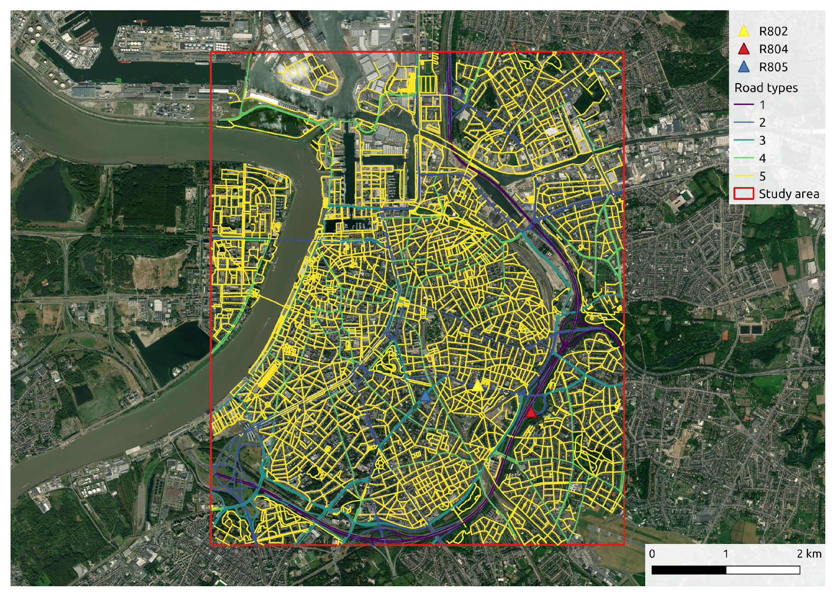
The mobile air quality monitoring campaign was conducted in the city of Antwerp from January 2018 to October 2021. It is the most populous city center in Belgium with a population of 529,417. There is a six-lane high-speed ring road that bypasses most of the city center and crosses urban residential areas, providing connections to other cities. The high traffic volume and daily congestion on the ring road are the main local source of traffic-related air pollutants. We focus on the city center of Antwerp as shown in Figure 1, which has high population density, complex road network structure and diverse microenvironments.

Figure 1.
The location of study area in the city center of Antwerp and the road network in the area of interest. The locations of three stationary regulatory monitoring stations are marked by different colored triangles.
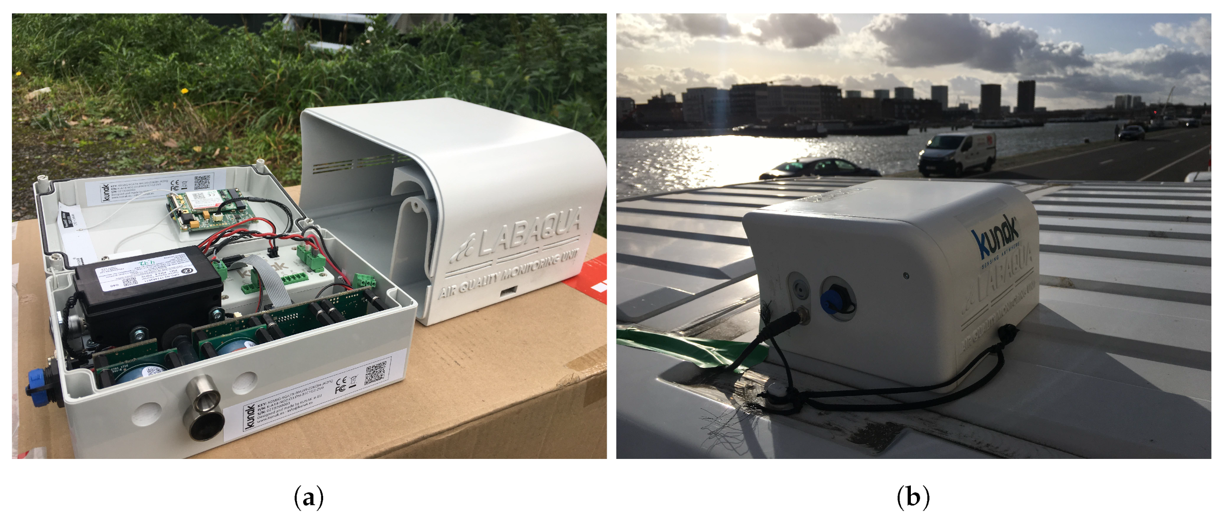
The Kunak AIR mobile sensor boxes were installed on 17 postal vans for opportunistic air quality monitoring in Antwerp (https://www.imeccityofthings.be/en/projecten/bel-air, accessed on 10 April 2022). A Kunak sensor box is equipped with three types of Alphasense sensors for measuring the concentration of particulate matter (PM1, PM2.5, PM10; OPC-N3), nitrogen dioxide (NO2; NO2-B43F) and ozone (O3; OX-B431), in-built sensors for measuring temperature and relative humidity of the environment, as well as a GPS for logging geographical coordinates (see Figure 2a) These sensors are continuously powered by a 12 V power supply from the vehicle battery and are equipped with LTE-M connectivity. The sensors also include a property algorithm to correct for the influence of environmental context and cross-interference between gases [45]. There is mobile housing provided by LABAQUA surrounding each Kunak sensor box to reduce the impact of turbulent airflow on sensors while the vehicle is in motion (see Figure 2b).
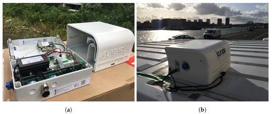
Figure 2.
The Kunak AIR mobile sensor system used in this paper. (a) A Kunak sensor box contains three types of Alphasense sensors for measuring the concentration of PM1, PM2.5, PM10 (OPC-N3), NO2 (NO2-B43F) and O3 (OX-B431), in-built sensors for measuring environmental temperature and relative humidity, as well as a GPS device. (b) The Kunak sensor box with a mobile housing is mounted on the roof of a postal van.
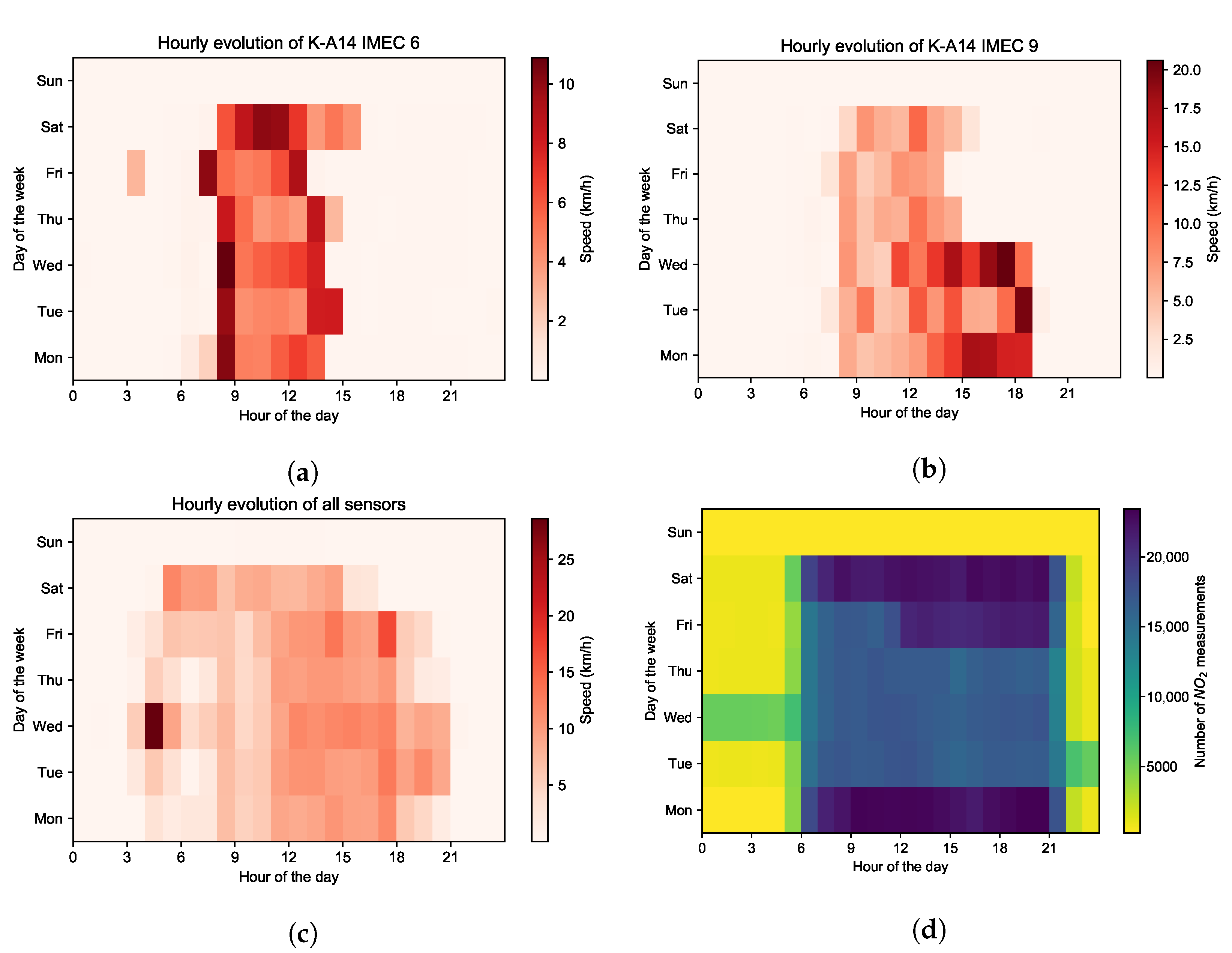
Given the operating characteristics of postal vans, the sampling campaign is generally conducted from 6:00 to 23:00 on weekdays and Saturday (see Figure 3), with relatively random sampling routes. The sampling interval is configured to 10 s during the daytime when the vehicle is operating and 10 min at night when the vehicle is parked, in order to avoid unnecessary power consumption. As a result, air quality data are captured every 10 s as the vehicle travels, including the concentrations of multiple air pollutants (PM1, PM2.5, PM10, NO2 and O3), the ambient temperature and relative humidity, together with the corresponding GPS coordinates and timestamps. The obtained temperature and relative humidity are mainly used to correct the influence of environmental context on sensors and reduce the uncertainty of the sensors.

Figure 3.
(a) The hourly evolution of the speed of mobile sensor K-A14 IMEC 6, (b) mobile sensor K-A14 IMEC 8 and (c) all mobile sensors during each day of the week on May 2021. (d) The hourly evolution of the number of NO2 measurements collected by all mobile sensors during each day of the week on May 2021.
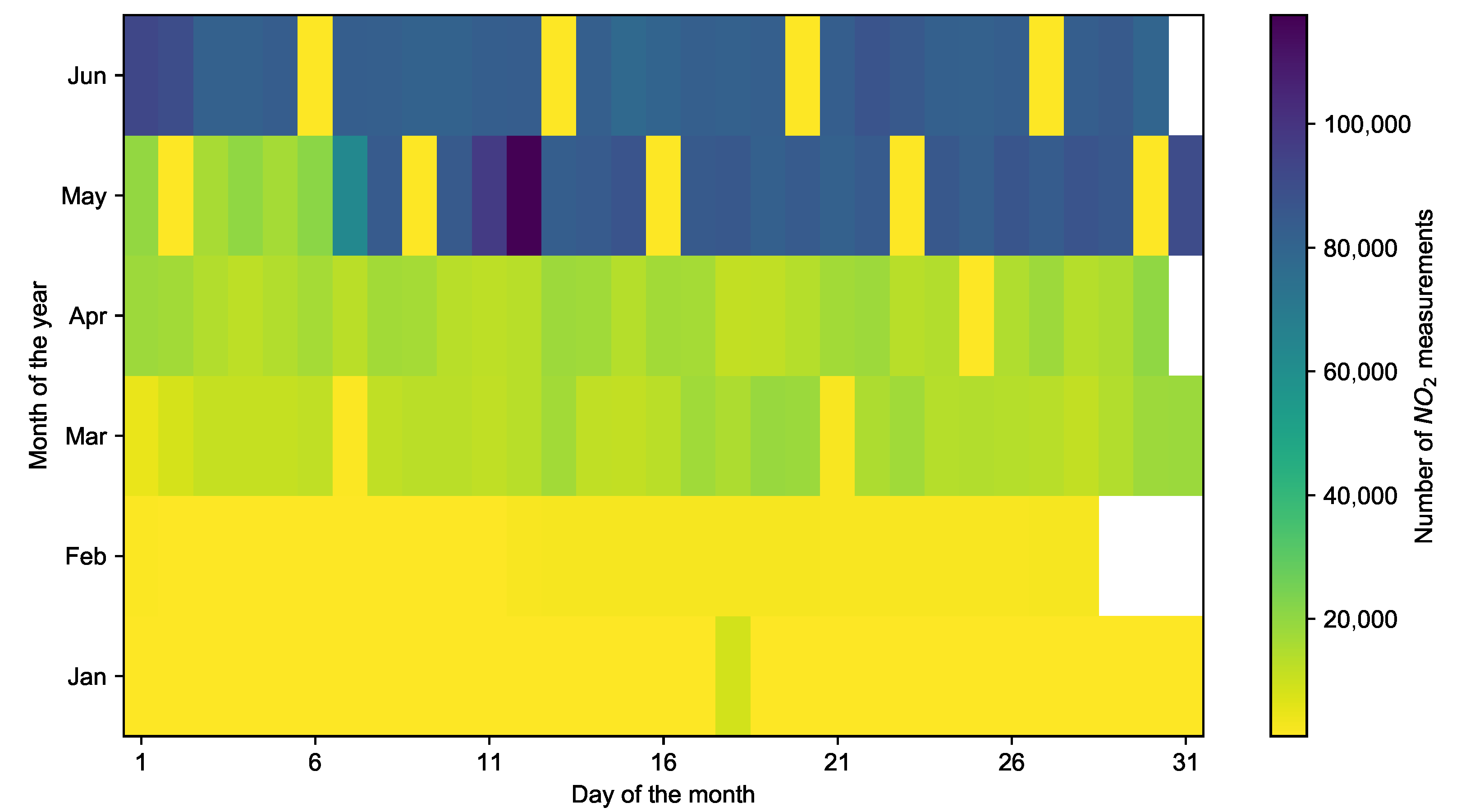
Figure 4 indicates the number of NO2 measurements collected by mobile sensors per day during the mobile monitoring campaign from January to June 2021, from which we can observe a relatively high amount of data collected in May and June. Considering that the company HERE Technologies (https://www.here.com/, accessed on 10 April 2022) only provided traffic flow for a maximum of 30 days, we select data from May and June for the subsequent data processing procedures. Based on the processed data, we then create a dataset by selecting 30 days with the most measurements and highest spatial coverage.
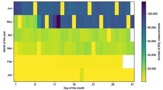
Figure 4.
The number of NO2 measurements collected by all mobile sensors per day from January to June 2021.
2.2. Data Processing
As the first step in data processing, we eliminate measurements that fall outside the study area and measurements collected outside working hours, which are meaningless because the vehicles are simply parked in the parking lot during these hours. In urban environments, the locations determined by GPS are typically slightly off-track due to the reflection of signals from high buildings and the synchronization of the measuring device [46]. Thus, map matching is employed to improve the accuracy of the GPS coordinates. For this, we assume all vehicle samples are taken on roads, and we correct GPS positions by projecting to the nearest road, as long as this correction is less than a threshold τ. Here we set the maximum distance τ as 30 m, referring to [46].
Next we aggregate the data in both time and spatial dimension to construct the air quality inference model and ultimately generate the fine-grained air quality map. Spatially, the road network in the study area is divided into road segments of approximately m in length. We represent each segment by its centroid coordinates; thus we obtain N centroids , where N is the number of road segments. In the time dimension, we quantize the timestamps of the measurements into uniform time slots of duration , resulting in a set of T time slots . Consequently, for a given time slot , all measurements located on the road segment i are allocated to the corresponding segment centroid .
Furthermore, we regard the mean value of these measurements as the measured value at the location in the time slot . To ensure data quality, we calculate the mean value based on at least four 10-s measurements (based on the previously mentioned sampling interval of 10 s), which covers approximately 100 m at an average speed of 2.47 m/s for all mobile sensors. Accordingly, we set to 100 m. In addition, we set to 1 h so that we can compare the inferred measurements with the reference measurements from the fixed monitoring station subsequently.
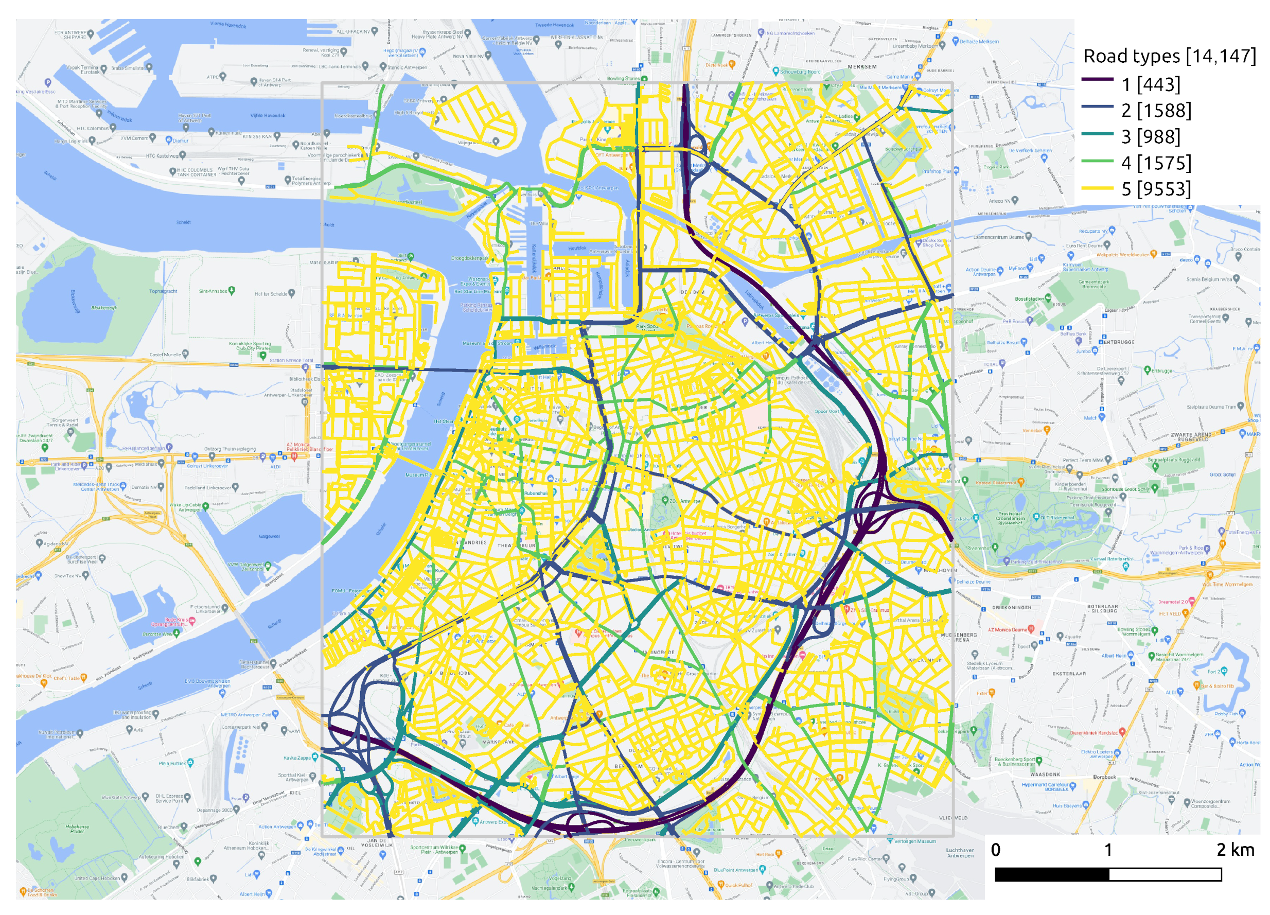
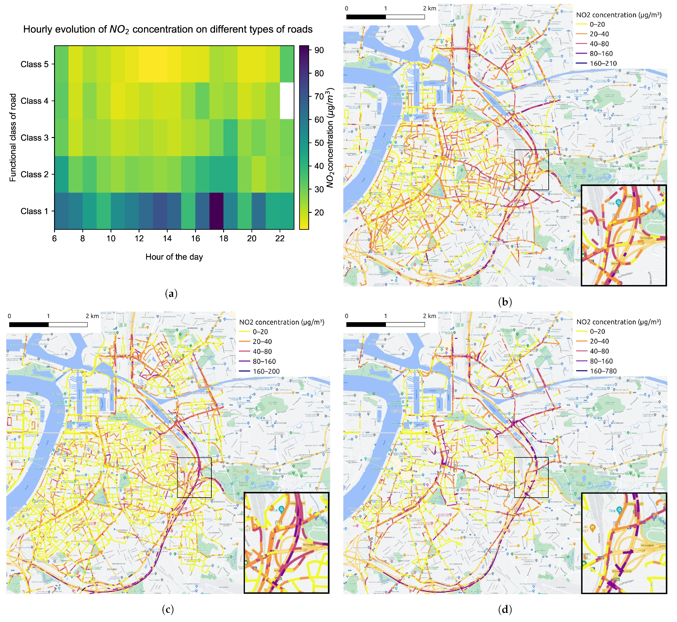
Table 1 shows the number of measurements after data processing procedures. The data aggregation process yields 176,460 measurements at 9550 different locations (from which a spatial coverage of 67.5% can be derived) for 884 working hours in May and June 2021. Some insights into the distribution of NO2 concentration can already be drawn using these aggregated NO2 measurements. Figure 5 categorizes the road segments into five functional classes, with Class 1 representing main roads, Class 2 and Class 3 representing primary roads I and II, Class 4 representing secondary roads, as well as Class 5 representing local roads within neighborhoods. Figure 6 displays the temporal and spatial distribution of NO2 in the city center of Antwerp during May and June 2021. The diurnal pattern of the NO2 distribution can be identified from Figure 6a. Combined with the map of road types given in Figure 5, it can be observed that on all types of roads, except the ring road, the NO2 concentration is relatively high during morning rush hours, falls back during midday and rises again during evening rush hours. It is worth noticing that the morning peak is more concentrated from 6:00 to 9:00 and has a small drop at 7:00, which may correspond to the diverse commuting time. As for the evening peak, it keeps climbing from 16:00 to 19:00, and after a little trough, it goes up slightly at 9:00 and 10:00. These two peaks coincide with the end times of work and entertainment activities, respectively. Figure 6b–d depicts the spatial distribution of NO2 during the morning rush hours, midday hours and evening rush hours, respectively. The daily pattern that NO2 concentration on road network fluctuates up and down over time is illustrated more clearly.

Table 1.
The number of NO2 measurements after each data processing step.
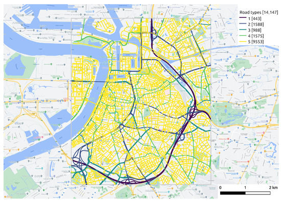
Figure 5.
The distribution of distinct road types. The quantity of different road types of road segments is shown by the numbers marked in brackets.
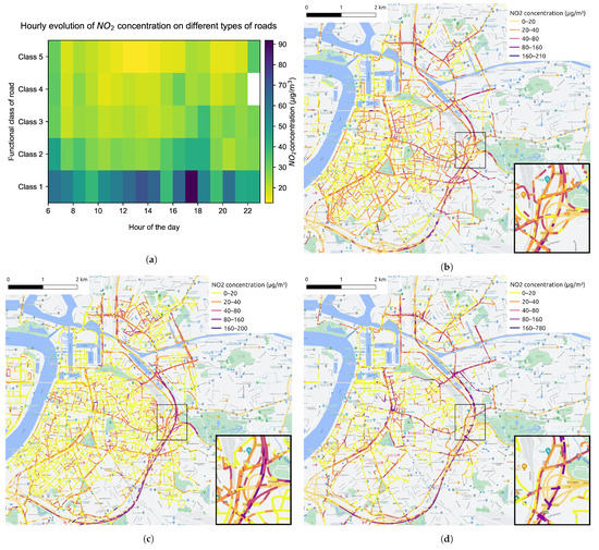
Figure 6.
(a) The hourly evolution of NO2 concentration on different types of roads. The map of average NO2 concentration at 100 m road segments during (b) morning rush hours (6:00∼10:00), (c) midday hours (11:00∼15:00) and (d) evening rush hours (16:00∼20:00), respectively.
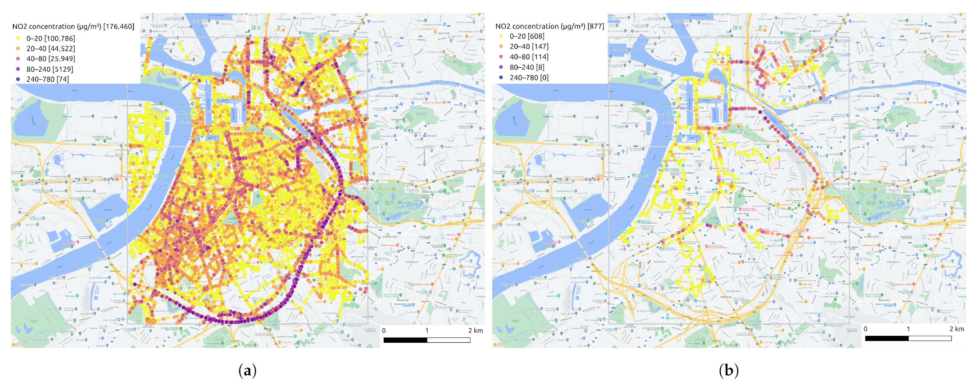
The map of all aggregated NO2 measurements after data processing steps is displayed in Figure 7a. The spatial coverage is high when all two-month measurements are put together. However, even for the hour with the most measurements among the two months (see Figure 7b), it is clear that the collected mobile measurements are still too sparse for fine-grained air quality mapping. For example, the majority of the measurements are located on the main roads, while the other areas have much fewer measurements. To tackle this issue, we develop an air quality inference model in Section 2.3.2 to create a fine-grained air quality map from these sparse measurements.
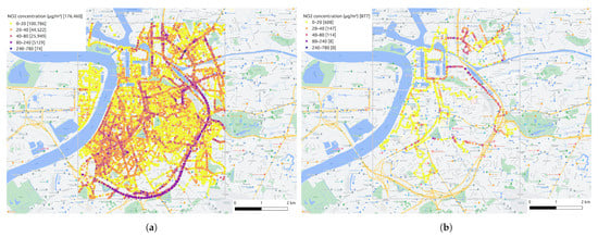
Figure 7.
(a) The map of all aggregated NO2 measurements after data processing procedures. (b) The map of aggregated NO2 measurements at 11:00 on 9 June 2021. The color bar represents various NO2 concentration level and the number followed means the amount of measurements at that level.
2.3. Methodology
2.3.1. Contextual Features
As mentioned earlier, contextual features have the capability of impacting the distribution of NO2 concentration, making contextual features critical information to build an air quality inference model. In general, depending on the type of contextual features, they can be classified into three categories:
- Time variant but space invariant: contextual features change over time but remain constant within a certain region. Meteorology belongs to this category, as it can change instantaneously during a day but can differ slightly across a city. The meteorological features we consider of interest are temperature, relative humidity, wind speed, and wind direction, owing to their important influence on the dispersion and transport processes of air pollutants. We acquired the hourly aggregated meteorological data from a stationary monitoring station (M802) in Antwerp provided by the Flanders Environment Agency (VMM). These data can be downloaded from VMM’s website (https://www.vmm.be/, accessed on 10 April 2022).
- Space variant but time invariant: contextual features change according to geographical location but remain unchanged over a short period of time, such as a road network. Features, such as road type and speed limits, differ from segment to segment, but remain constant for a long time. We extract the road network of study area from OpenStreetMap (OSM) (https://www.openstreetmap.org/, accessed on 10 April 2022). Figure 5 displays the functional classes of road segments defined by the “Flanders Spatial Structure Plan” (Ruimtelijk Structuurplan Vlaanderen). Class 1 represents main roads, connecting between large areas and cities, which are always busy with high traffic volumes and fast speeds. Class 2 denotes primary roads I, serving as a supplement to main roads. Class 3 indicates primary roads II that give access to the city center and limit traffic flow by increasing traffic signals. Class 4 indicates secondary roads that link different small towns. Class 5 represents local roads with access to communities.
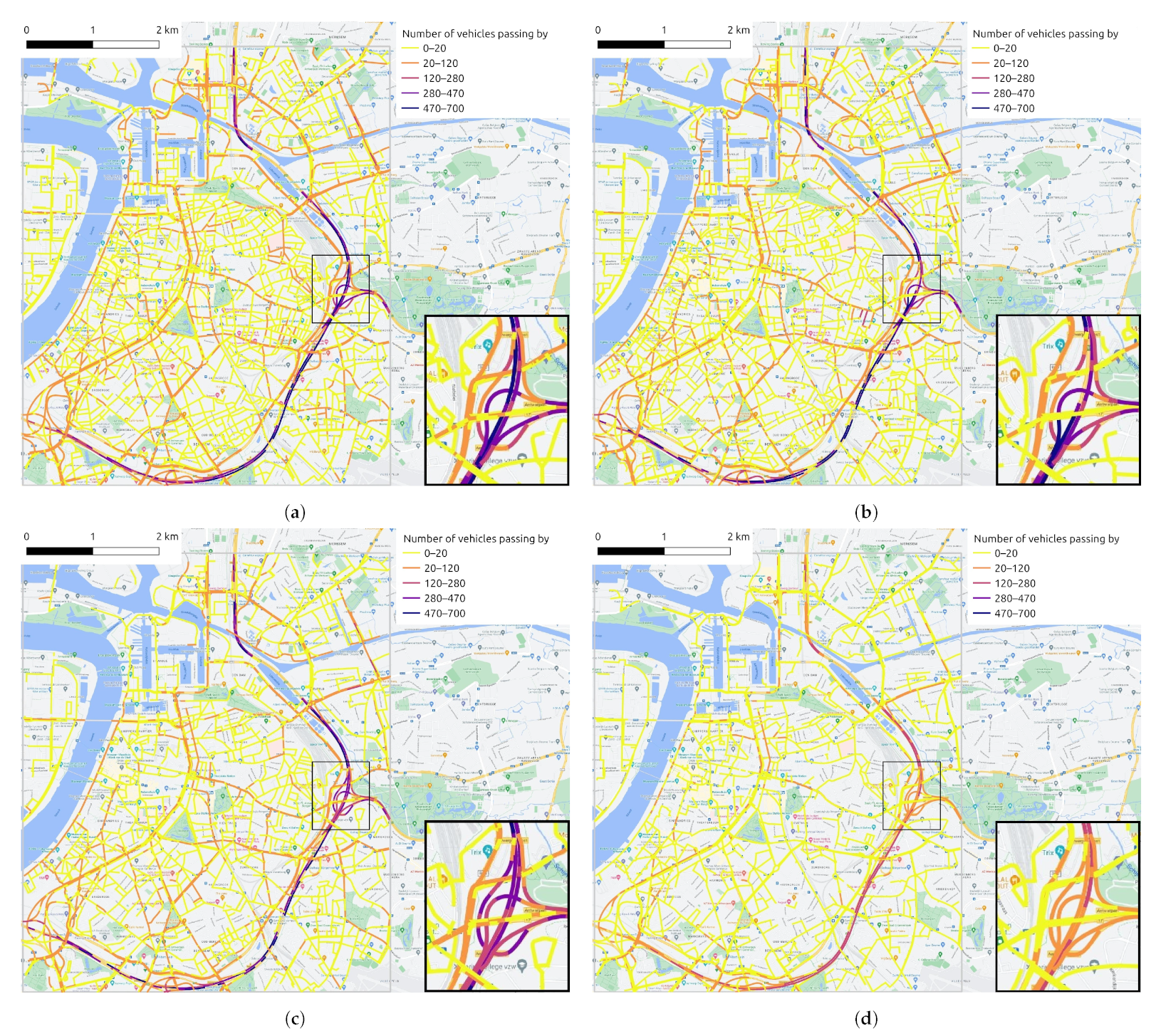
- Time- and space variant: these contextual features change both over time and space. For example, traffic flow can vary considerably by road segment and time slot. The average speed of vehicles on the road and the traffic density are the two traffic features we concern mainly. The traffic flow data used in this study are provided by the company HERE Technologies (https://www.here.com/, accessed on 10 April 2022).As an example, Figure 8 provides the evolution of traffic volumes on the road network at four time points (9:00, 13:00, 17:00 and 21:00) during a given day (10 June 2021). Taking into account road types in Figure 5, it is easy to find the temporal variation and spatial distribution of traffic flow. Due to the capacity and location of roads, it is not surprising that the six-lane highway ring road carries the heaviest traffic flow, followed by main roads with relatively more vehicles, and finally, the smaller traffic volume is on minor roads in some neighborhoods. In addition, as it was a weekday, the morning peak (Figure 8a) and evening peak (Figure 8c) contributed heavily to the traffic flow. The road network was still busy during the midday hour (Figure 8b) but less so than in the morning rush hour, and there was much less traffic volume when night fell (Figure 8d).
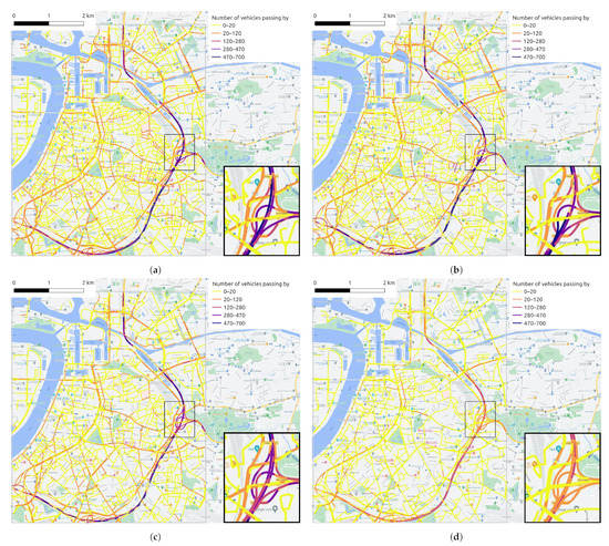 Figure 8. Traffic volume (i.e., the number of vehicles passing per 5 min) on road segments in study area at (a) 9:00, (b) 13:00, (c) 17:00 and (d) 21:00 on 10 June 2021. A small region is enlarged for better visualization in the bottom right corner.
According to the temporal and spatial distribution of NO2 shown in Figure 6 and different functional classes of roads displayed in Figure 5, it can be discovered that the NO2 concentration on the ring road is higher compared with other roads. Outside the morning and evening rush hours, the NO2 concentration on the ring road is still quite high at noon. In addition, the NO2 concentration on primary roads is also higher than that on local roads between neighborhood most of the time, which makes the temporal distribution of NO2 on different types of roads shown as Figure 6a appear as a gradient effect. Combined Figure 6 with Figure 8, it can be recognized that the distribution of the NO2 concentration on road network is generally consistent with the distribution of traffic volume. It is mentioned earlier that automobile emissions on the roadways are the primary and direct source of NOx, so the variation of traffic flow has a direct impact on the NO2 distribution. Furthermore, the functional class of the road is assigned based on its connectivity and accessibility, which can reflect the traffic volume on the road, so the road type has an indirect impact on NO2 distribution.
2.3.2. Creating a Fine-Grained Air Quality Map from Sparse Measurements
Based on the opportunistic mobile monitoring campaign and data processing procedures, we derived a large number of aggregated NO2 measurements. All aggregated NO2 measurements are used to construct a series of NO2 concentration maps , where represents the NO2 concentration map for a certain time slot and consists of NO2 measurements at time slot t. By accumulating all NO2 concentration maps, the collected measurements cover all time slots and majority of road segments as shown in Figure 7a. However, when extracting a NO2 concentration map for a specific time slot, the collected measurements are still relatively sparse (see Figure 7b), because it is difficult for a limited number of mobile sensors to traverse all road segments in the entire region in one hour. Thus, we can only obtain a series of sparse NO2 concentration maps based on the mobile measurements.
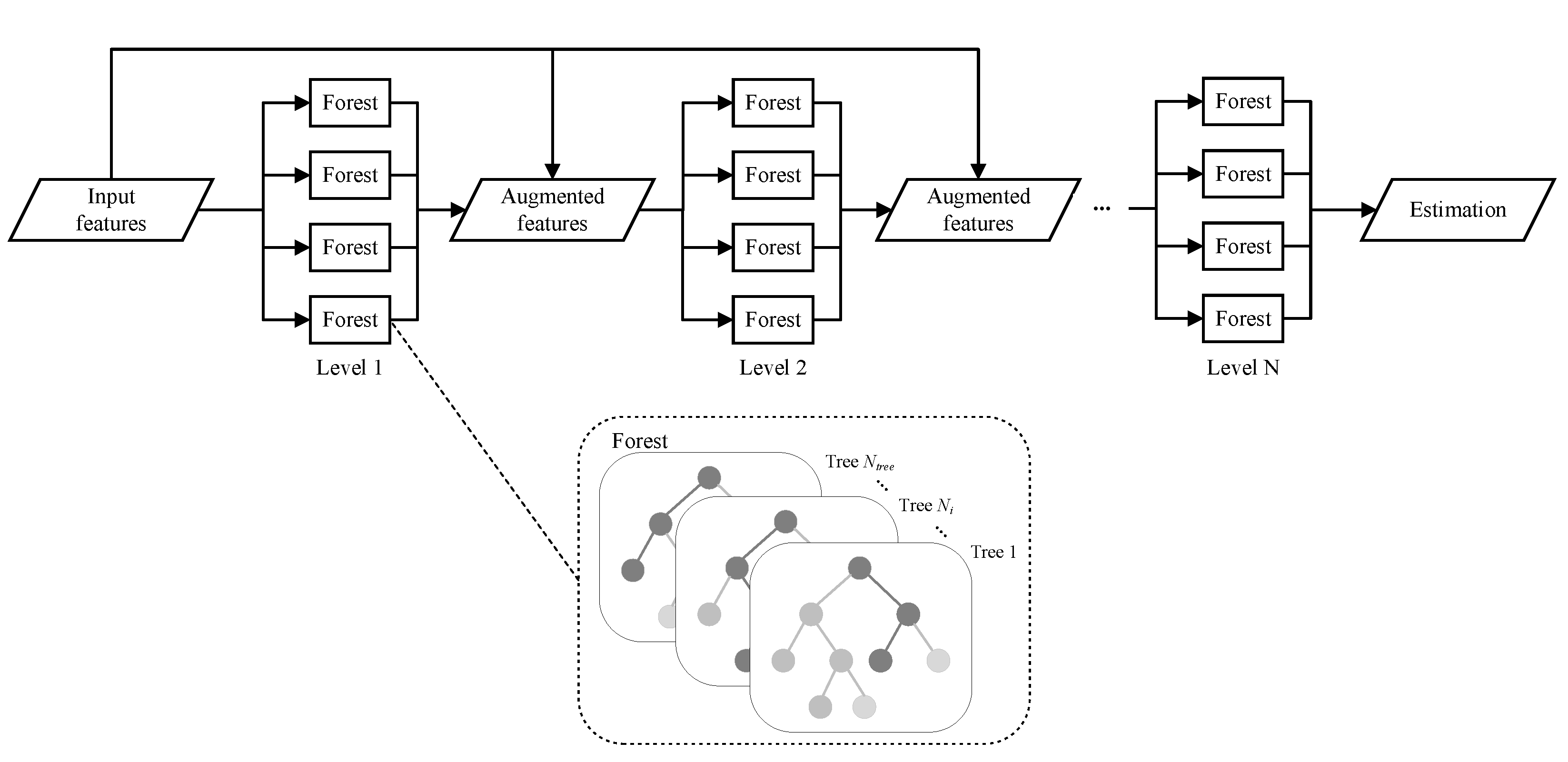
Aiming to generate a complete fine-grained NO2 concentration map from sparse mobile measurements and various contextual features, we propose a context-aware locally adapted deep forest (CLADF) model. As an upgraded and improved version of our previously proposed geographically context-aware random forest (GCRF) model in [37], the CLADF model introduces deep forest (DF) [47], replacing the existing random forest (RF) [48] to construct context-aware local models, enabling representation learning by forests. Figure 9 illustrates the structure of deep forest. The GCRF model simply builds a local model for each measurement, which is prone to redundancy, as well as requires high computational and memory costs. To address these issues, the CLADF model first clusters all measurements according to the similarity of contextual features, and then builds a local model for the measurements within each cluster. Moreover, in terms of contextual features, the CLADF model incorporates traffic flow in addition to the meteorology and road network that have been considered in the GCRF model, due to the important contribution of on-road automobile emissions to NO2 concentrations and the local effect of traffic flow on the spatiotemporal variation of NO2 concentrations. As a result, the CLADF model improves accuracy, reduces redundancy and saves computational costs compared to the GCRF model. Figure 10 displays the workflow of the CLADF model. Overall, the whole process consists of three steps: input feature generation, global/local model construction and final estimation.

Figure 9.
Illustration of the deep forest and its forest structure. Assume that there are N levels in deep forest and each level has 4 forests. The input features are fed into the first level, and each forest in the first level generates the corresponding estimations. These estimations will be concatenated with original features to compose augmented features, which are input to the next level until the final level derives the final outcome. Moreover, the structure of each forest is shown in the dashed box. A random part of input features is selected to build decision trees, and the estimations generated by all trees in the same forest are averaged.
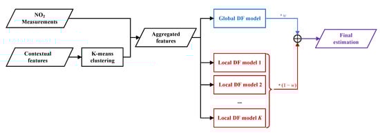
Figure 10.
The workflow of proposed CLADF model.
In the phase of input feature generation, we put all NO2 measurements into a vector and take their corresponding contextual features as a set of vectors , where , N is the total number of measurements and F is the dimension of contextual features. The following contextual features are considered in this study: day of the week, hour of the day, geographical location, temperature, relative humidity, wind speed, wind direction, road type and traffic density. In order to find measurements that have similar contextual features, K-means clustering algorithm is used to classify each measurement into one of clusters based on its contextual features . The objective of K-means algorithm is to find a set of clusters for all measurements based on their contextual features that minimizes the within-cluster sum-of-squares criterion:
where is the mean of contextual features of measurements in the cluster . We need to specify the number of clusters K which determines the number of local models and also affects the performance of the CLADF model. Thus, we build the CLADF models using clusters with different K values and find the optimal K that minimizes the performance metric RMSE mentioned in Section 2.4.2 of the CLADF model. The aggregated features are generated by merging NO2 measurements and their contextual features on the corresponding timestamps and geographical locations. Therefore, the aggregated features fed into the global/local model are represented as a series of vectors , where .
In order to develop the global/local model, there are two branches in parallel. The first branch feeds all aggregated features A into a deep forest to train a global model. The other branch utilizes the aggregated features in each cluster to train a local model k, . To infer the unmeasured NO2 concentration on a certain location at a specific time slot, its corresponding contextual features are used to find the closest cluster in the training set it belongs to. Then, the global model outputs an estimated NO2 concentration by feeding its contextual features , which is derived from all measurements. The local model for the cluster it belongs to produces another NO2 estimation , which is inferred from the measurements sharing similar contextual features with it, such as the NO2 concentration at another location with similar traffic flow during the same time slot. The global estimation reflects the heterogeneity of all measurements, and the local estimation demonstrates the homogeneity of similar measurements.
Finally, we introduce a weighting factor w to combine these two estimations into the final estimation . In this way, the final prediction of the overall CLADF model integrates the advantages of both global and local estimations. For the setting of the weighting factor w, we calculate the performance metric RMSE (see Section 2.4.2) of the CLADF model with different w ranging from 0 to 1 with step 0.1 and choose the optimal w that minimizes the RMSE of the CLADF model.
2.4. Performance Evaluation
2.4.1. Validation Experiments
Given that the company HERE Technologies only shared traffic flow for up to 30 days as mentioned in Section 2.1, we select 30 days with the most measurements and highest spatial coverage among May and June 2021, and create a dataset accordingly. The dataset that consists of hourly aggregated NO2 measurements from these 30 days combined with their corresponding contextual features (including day of the week, hour of the day, geographical location, temperature, relative humidity, wind speed, wind direction, road type and traffic density) is used for the validation experiments of the CLADF model and different baseline models.
In our study area, there are six stationary monitoring stations provided by VMM. They can be divided into three types of microenvironments according to their locations in the road network, namely, roadside, street canyon and highway. Removing stations close to each other, we consider three typical fixed-location monitoring stations located at roadside (R802), street canyon (R805) and highway (R804) respectively in the leave-one-station-out validation experiments, to compare the performance of various air quality inference models in different microenvironments. First, hourly measurements from these three stationary monitoring stations are concatenated with hourly aggregated measurements from mobile sensors. Next, for each stationary monitoring station, the measurements from this station and the mobile measurements at the same location are eliminated, and the remaining measurements located at other locations are used to train the model. Finally, the estimated values inferred from the model are compared with the ground-truth values from this reference station to calculate various performance metrics. This leave-one-station-out validation experiment is repeated for each of three reference stations. For each reference station, the number of NO2 measurements in training set and test set is shown in Table 2.
Table 2.
The number of NO2 measurements in training set and test set for each validation experiment.
With the aim of evaluating the effect of contextual features on the performance of the model and comparing the inference ability of the model under different scenarios, 5-fold cross validation experiments based on road functional class were conducted. All hourly aggregated measurements are split into five groups according to road functional class. In each group, we randomly select 75% of measurements as the training set, with the remaining 25% of measurements as the test set. This cross validation experiment is iterated for each group from Functional Class 1 through 5. Table 2 presents the number of NO2 measurements in the training set and test set for each class.
2.4.2. Performance Metrics
The results of the validation experiments are evaluated by the following performance metrics: root mean squared error (RMSE), mean absolute error (MAE), index of agreement (IA), accuracy, correlation coefficient (r), normalized mean bias (NMB) and normalized mean standard deviation (NMSD), which are calculated as follows:
where is the measured value, is an estimated value, and are the mean of measured values and the mean of estimated values, and and are the standard deviation of measured values and the standard deviation of estimated values. RMSE and MAE represent the difference between the estimated and measured values for measuring the errors in air quality inference, so the smaller these two metrics, the better. IA and accuracy indicate the similarly between the estimated and measured values ranging from 0 to 1, where 1 represents perfect agreement. Correlation coefficient r reflects the linear correlation between the estimated and measured values and ranges in [−1, 1], where 0 means no correlation and 1 (or −1) means the perfect linear (anti) correlation. IA and accuracy are independent of the relationship between variables while r only represents the linear relationship, and hence we consider IA and accuracy in preference to r. NMB denotes the normalized bias of mean estimated values compared to mean measured values, and NMSD denotes the normalized difference between standard deviation of estimated values and standard deviation of measured values. The positive and negative of both metrics show whether the model is over- or underestimated.
Although the above statistical performance metrics can generally provide an insight into the performance of a model, they cannot indicate whether the model has reached a level of quality that can be applied. Here, the model quality indicator (MQI) introduced by [49] determines whether a model meets the minimum level of quality for policy use. The calculation is as follows:
where is 0.24, is 200 g/m and is 0.2 for NO2 according to their recommended settings. The proportionality coefficient is set to 2, which means that the deviation between the estimated values and measured values is allowed to be as large as twice the measurement uncertainty . MQI is the main performance indicator, and when , the quality of the model is able to achieve the objective.
3. Results and Discussion
3.1. Model Performance
In the experiments of this study, the benchmark methods used for performance comparison with the proposed CLADF model are support vector regression, extreme gradient boosting, random forest and deep forest. Support vector regression (SVR) [50] is an extension of the support vector machine (SVM) applied to regression problems. The extreme gradient boosting (XGBoost) [51] is based on gradient boosting decision tree (GBDT) but with some optimization to make it efficient, flexible and portable. GBDT is a boosting ensemble algorithm that incorporates multiple weak learners into a single strong learner. In general, GBDT is an additive model that can be considered a linear addition of many base methods (i.e., CART regression trees). XGBoost has been reported as a state-of-the-art machine learning method to derive urban air quality maps [34]. Random forest (RF) [48] combines the ensemble learning method with the decision tree framework to create a number of decision trees from the data, averaging the results to output a new result that often leads to strong predictions. Deep forest (DF) [47] is a decision tree ensemble algorithm with a cascade structure that enables representation learning through forests. Meanwhile, multi-granularity scanning can strengthen its representation learning capability, potentially making deep forest context aware. Its hyperparameters are much fewer than deep neural networks, and its complexity can be auto-determined based on the data.
The hyper-parameters of different methods for optimizing the performance metrics are set as follows:
- SVR model: radial basis kernel function (rbf) with kernel coefficient and regularization parameter C = 1.
- XGBoost model: number of gradient boosted trees = 200.
- RF model: number of trees in the forest = 200.
- DF model: maximum number of cascade layers = 20, number of estimator in each cascade layer = 4, number of trees in each estimator = 200.
- Proposed CLADF model: number of estimator in each cascade layer = 4, number of trees in each estimator = 200, weighting factor , number of clusters K = 120, 200, 40 for R802, R804, R805 respectively in leave-one-station-out validation experiments and K = 5, 20, 10, 10, 40 for Class 1 to 5 in the five-fold cross validation experiments based on road type.
The results of leave-one-station-out validation experiments are illustrated in Table 3. For all three reference stations, the proposed CLADF model stands out among all compared methods. In general, the CLADF model decreases RMSE from 20.12 to 15.95 μg/m3, increases Acc. from 0.52 to 0.61 with respect to accuracy, and improves both IA (0.54 → 0.6) and r (0.36 → 0.45) in terms of correlation. Additionally, it fulfills the quality criterion required for policy purposes, i.e., that MQI ≤ 1 [49]. It is worth noting that the XGBoost model performs relatively well on most metrics (only worse than CLADF model) for R802 and R805; however, it performs worse (only better than RF model) at R804.
Table 3.
Comparison of performance metrics of methods at three different reference stations.
As shown in Figure 1, these reference stations correspond to different microenvironments: roadside (R802), street canyon (R805) and highway (R804), respectively, so by comparing the performance of various methods at different stations, we can observe the impact of training data on model performance. All methods misplay at R804 and give the worst results of three experiments. Station R804 poses a challenge for all methods since the limited number of measurements from mobile sensors are collected from the ring road and due to the far distance (40 m) from the nearest road segment compared to the other two reference stations located close to roads (12 m for R802 and 6 m for R805). Moreover, the contextual features of measurements on the ring road are special and less similar to other measurements. Nevertheless, the proposed CLADF model outperforms other methods on all metrics, and even improves many metrics more obviously (reducing RMSE by ~29% from 32.85 to 23.28 and enhancing Acc. by 50% from 0.36 to 0.54) than at the other two stations. Consequently, our proposed model not only performs well on datasets with abundant training data, but also performs excellently on datasets with limited training data.
Table 4 demonstrates the comparison of performance metrics of different methods in 5-fold cross-validation experiments based on road type. The five sub-datasets divided by the road functional class represent five diverse scenarios. The functional class of the road is defined in the “Flanders Spatial Structure Plan” (Ruimtelijk Structuurplan Vlaanderen). Class 1 indicates main roads (i.e., the ring road in this case), which link large regions and cities with high traffic flow, big traffic capacity and numerous heavy-duty vehicles, such as coaches and trucks. Class 2 indicates primary roads I, which complement the connection function of main roads. Class 3 indicates primary roads II, which provide access to central urban areas and have increased traffic signals. Class 4 indicates secondary roads, which mainly connect small towns and allow mixed traffic. Class 5 indicates local roads, which are accessible to communities and have lower traffic speeds. Overall, the CLADF model shows better performance than the other methods on all metrics in all scenarios. The DF and RF model are the next best and perform more comparably, while the SVR model has the worst performance.
Table 4.
Comparison of performance metrics of models on five different types of roads.
As illustrated in Table 2, the number of measurements in Class 1 is much smaller than in Class 5. Due to the fact that there is a discrepancy in the number of different types of roads, most measurements from mobile sensors were collected from local roads and secondary roads, with a minority from primary roads and very few from highways. It is evident from Table 4 that maximum RMSE (21.8∼37.33 μg/m3) and MAE (15.4∼27.91 μg/m3) are observed in Class 1 as there are fewest measurements, while IA, Acc. and r are generally high, owing to the homogeneity of measurements in highways. In contrast, Class 5 indicates small roads between neighborhood, which is of a big amount but widely scattered, leading to the minimum RMSE (12.39∼17.09 μg/m3 and MAE (7.98∼11.29 μg/m3), but not the highest IA, Acc. and r of all classes. The most obvious enhancement of the CLADF model for RMSE and MAE is observed in Class 1 with decreases of 5% and 6.7%, respectively. This validation experiment demonstrates that the CLADF model can be applied not only to scenarios with sufficient data, but also to those with sparse data.
In order to validate the necessity of the local model, the weighting factor w is set to 1. In this case, the CLADF model degrades to the global model (i.e., DF model) without considering the local model. It is evident that all performance metrics of the CLADF model are superior to the global model in all scenarios as shown in Table 3 and Table 4.
4. Conclusions
In this study, based on NO2 measurements collected from an opportunistic mobile monitoring campaign in Antwerp and three categories of contextual features including meteorology, road network and traffic flow, we propose an air quality inference model named CLADF to create fine-grained air quality maps. The CLADF model utilizes deep forest to construct a local model for each cluster that members have similar contextual features, as well as emphasizing the role of traffic flow as a contextual feature. A variety of validation experiments demonstrate that the CLADF model outperforms various baseline methods in all performance metrics.
Author Contributions
Methodology, Research and writing: X.Q.; Research supervision: W.P., N.D. and V.P.L.M.; Data processing: X.Q., T.H.D. and E.R.B.; Critical review: J.H., T.H.D. and E.R.B. All authors have read and agreed to the published version of the manuscript.
Funding
This research was funded by imec Belgium through AAA funding, by the Internet of Things (IoT) team of imec-Netherlands under the project EI2 and by the Flemish Government (AI Research Program).
Data Availability Statement
Not applicable.
Conflicts of Interest
The authors declare no conflict of interest.
References
- World Health Organization. WHO Global Air Quality Guidelines: Particulate Matter (PM2.5 and PM10), Ozone, Nitrogen Dioxide, Sulfur Dioxide and Carbon Monoxide; World Health Organization: Geneva, Switzerland, 2021. [Google Scholar]
- World Bank and Institute for Health Metrics and Evaluation. The Cost of Air Pollution: Strengthening the Economic Case for Action; World Bank: Washington, DC, USA, 2016. [Google Scholar] [CrossRef]
- Samoli, E.; Peng, R.; Ramsay, T.; Pipikou, M.; Touloumi, G.; Dominici, F.; Burnett, R.; Cohen, A.; Krewski, D.; Samet, J.; et al. Acute Effects of Ambient Particulate Matter on Mortality in Europe and North America: Results from the APHENA Study. Environ. Health Perspect. 2008, 116, 1480–1486. [Google Scholar] [CrossRef] [PubMed] [Green Version]
- Beelen, R.; Raaschou-Nielsen, O.; Stafoggia, M.; Andersen, Z.J.; Weinmayr, G.; Hoffmann, B.; Wolf, K.; Samoli, E.; Fischer, P.; Nieuwenhuijsen, M.; et al. Effects of Long-term Exposure to Air Pollution on Natural-Cause Mortality: An Analysis of 22 European Cohorts within the Multicentre ESCAPE Project. Lancet 2014, 383, 785–795. [Google Scholar] [CrossRef]
- Burnett, R.; Chen, H.; Szyszkowicz, M.; Fann, N.; Hubbell, B.; Pope, C.A.; Apte, J.S.; Brauer, M.; Cohen, A.; Weichenthal, S.; et al. Global estimates of mortality associated with long-term exposure to outdoor fine particulate matter. Proc. Natl. Acad. Sci. USA 2018, 115, 9592–9597. [Google Scholar] [CrossRef] [PubMed] [Green Version]
- Chen, K.; Breitner, S.; Wolf, K.; Stafoggia, M.; Sera, F.; Vicedo-Cabrera, A.M.; Guo, Y.; Tong, S.; Lavigne, E.; Matus, P.; et al. Ambient carbon monoxide and daily mortality: A global time-series study in 337 cities. Lancet Planet. Health 2021, 5, e191–e199. [Google Scholar] [CrossRef]
- Carvalho, H. The air we breathe: Differentials in global air quality monitoring. Lancet Respir. Med. 2016, 4, 603–605. [Google Scholar] [CrossRef]
- Karner, A.A.; Eisinger, D.S.; Niemeier, D.A. Near-Roadway Air Quality: Synthesizing the Findings from Real-World Data. Environ. Sci. Technol. 2010, 44, 5334–5344. [Google Scholar] [CrossRef]
- Marshall, J.D.; Nethery, E.; Brauer, M. Within-Urban Variability in Ambient Air Pollution: Comparison of Estimation Methods. Atmos. Environ. 2008, 42, 1359–1369. [Google Scholar] [CrossRef]
- Tang, H.; Apon, F. Integrative Air Quality Management Airshed by Using Multigas Passive Sampling Technology in Canada. WIT Trans. Ecol. Environ. 2012, 162, 517–528. [Google Scholar]
- Rosario, L.; Pietro, M.; Francesco, S.P. Comparative Analyses of Urban Air Quality Monitoring Systems: Passive Sampling and Continuous Monitoring Stations. Energy Procedia 2016, 101, 321–328. [Google Scholar] [CrossRef]
- Zou, B.; Li, S.; Zheng, Z.; Zhan, B.F.; Yang, Z.; Wan, N. Healthier Routes Planning: A New Method and Online Implementation for Minimizing Air Pollution Exposure Risk. Comput. Environ. Urban Syst. 2020, 80, 101456. [Google Scholar] [CrossRef]
- Luo, J.; Boriboonsomsin, K.; Barth, M. Consideration of Exposure to Traffic-related Air Pollution in Bicycle Route Planning. J. Transp. Health 2020, 16, 100792. [Google Scholar] [CrossRef]
- Apparicio, P.; Gelb, J.; Carrier, M.; Mathieu, M.È.; Kingham, S. Exposure to Noise and Air Pollution by Mode of Transportation during Rush Hours in Montreal. J. Transp. Geogr. 2018, 70, 182–192. [Google Scholar] [CrossRef]
- Isakov, V.; Touma, J.S.; Khlystov, A. A method of assessing air toxics concentrations in urban areas using mobile platform measurements. J. Air Waste Manag. Assoc. 2007, 57, 1286–1295. [Google Scholar] [CrossRef] [PubMed] [Green Version]
- Apte, J.S.; Messier, K.P.; Gani, S.; Brauer, M.; Kirchstetter, T.W.; Lunden, M.M.; Marshall, J.D.; Portier, C.J.; Vermeulen, R.C.; Hamburg, S.P. High-resolution air pollution mapping with Google street view cars: Exploiting big data. Environ. Sci. Technol. 2017, 51, 6999–7008. [Google Scholar] [CrossRef]
- Mueller, M.D.; Hasenfratz, D.; Saukh, O.; Fierz, M.; Hueglin, C. Statistical modelling of particle number concentration in Zurich at high spatio-temporal resolution utilizing data from a mobile sensor network. Atmos. Environ. 2016, 126, 171–181. [Google Scholar] [CrossRef]
- Kaivonen, S.; Ngai, E.C.H. Real-time air pollution monitoring with sensors on city bus. Digit. Commun. Netw. 2020, 6, 23–30. [Google Scholar] [CrossRef]
- Elen, B.; Peters, J.; Poppel, M.V.; Bleux, N.; Theunis, J.; Reggente, M.; Standaert, A. The Aeroflex: A Bicycle for Mobile Air Quality Measurements. Sensors 2013, 13, 221–240. [Google Scholar] [CrossRef]
- Franco, J.F.; Segura, J.F.; Mura, I. Air Pollution alongside Bike-Paths in Bogotá-colombia. Front. Environ. Sci. 2016, 4, 77. [Google Scholar] [CrossRef] [Green Version]
- McKercher, G.R.; Vanos, J.K. Low-Cost Mobile Air Pollution Monitoring in Urban Environments: A Pilot Study in Lubbock, Texas. Environ. Technol. 2018, 39, 1505–1514. [Google Scholar] [CrossRef]
- Hofman, J.; Samson, R.; Joosen, S.; Blust, R.; Lenaerts, S. Cyclist Exposure to Black Carbon, Ultrafine Particles and Heavy Metals: An Experimental Study along Two Commuting Routes near Antwerp, Belgium. Environ. Res. 2018, 164, 530–538. [Google Scholar] [CrossRef]
- Mead, M.; Popoola, O.; Stewart, G.; Landshoff, P.; Calleja, M.; Hayes, M.; Baldovi, J.; McLeod, M.; Hodgson, T.; Dicks, J.; et al. The Use of Electrochemical Sensors for Monitoring Urban Air Quality in Low-Cost, High-Density Networks. Atmos. Environ. 2013, 70, 186–203. [Google Scholar] [CrossRef] [Green Version]
- SM, S.N.; Yasa, P.R.; Narayana, M.; Khadirnaikar, S.; Rani, P. Mobile Monitoring of Air Pollution Using Low Cost Sensors to Visualize Spatio-Temporal Variation of Pollutants at Urban Hotspots. Sustain. Cities Soc. 2019, 44, 520–535. [Google Scholar] [CrossRef]
- Chen, G.; Knibbs, L.D.; Zhang, W.; Li, S.; Cao, W.; Guo, J.; Ren, H.; Wang, B.; Wang, H.; Williams, G.; et al. Estimating Spatiotemporal Distribution of PM1 Concentrations in China with Satellite Remote Sensing, Meteorology, and Land Use Information. Environ. Pollut. 2018, 233, 1086–1094. [Google Scholar] [CrossRef] [PubMed]
- Lin, C.; Labzovskii, L.D.; Mak, H.W.L.; Fung, J.C.; Lau, A.K.; Kenea, S.T.; Bilal, M.; Hey, J.D.V.; Lu, X.; Ma, J. Observation of PM2.5 Using a Combination of Satellite Remote Sensing and Low-Cost Sensor Network in Siberian Urban Areas with Limited Reference Monitoring. Atmos. Environ. 2020, 227, 117410. [Google Scholar] [CrossRef]
- Guttikunda, S.K.; Nishadh, K.; Jawahar, P. Air Pollution Knowledge Assessments (APnA) for 20 Indian Cities. Urban Clim. 2019, 27, 124–141. [Google Scholar] [CrossRef]
- Giani, P.; Castruccio, S.; Anav, A.; Howard, D.; Hu, W.; Crippa, P. Short-Term and Long-Term Health Impacts of Air Pollution Reductions from COVID-19 Lockdowns in China and Europe: A Modelling Study. Lancet Planet. Health 2020, 4, e474–e482. [Google Scholar] [CrossRef]
- Lim, C.C.; Kim, H.; Vilcassim, M.R.; Thurston, G.D.; Gordon, T.; Chen, L.C.; Lee, K.; Heimbinder, M.; Kim, S.Y. Mapping Urban Air Quality Using Mobile Sampling with Low-Cost Sensors and Machine Learning in Seoul, South Korea. Environ. Int. 2019, 131, 105022. [Google Scholar] [CrossRef]
- Mo, Y.; Booker, D.; Zhao, S.; Tang, J.; Jiang, H.; Shen, J.; Chen, D.; Li, J.; Jones, K.C.; Zhang, G. The Application of Land Use Regression Model to Investigate Spatiotemporal Variations of PM2.5 in Guangzhou, China: Implications for the Public Health Benefits of PM2.5 Reduction. Sci. Total Environ. 2021, 778, 146305. [Google Scholar] [CrossRef]
- Christopher, S.A.; Gupta, P. Satellite Remote Sensing of Particulate Matter Air Quality: The Cloud-Cover Problem. J. Air Waste Manag. Assoc. 2010, 60, 596–602. [Google Scholar] [CrossRef]
- Mogollón-Sotelo, C.; Casallas, A.; Vidal, S.; Celis, N.; Ferro, C.; Belalcazar, L. A Support Vector Machine Model to Forecast Ground-Level PM2.5 in a Highly Populated City with a Complex Terrain. Air Qual. Atmos. Health 2021, 14, 399–409. [Google Scholar] [CrossRef]
- Araki, S.; Shima, M.; Yamamoto, K. Spatiotemporal Land Use Random Forest Model for Estimating Metropolitan NO2 Exposure in Japan. Sci. Total Environ. 2018, 634, 1269–1277. [Google Scholar] [CrossRef] [PubMed]
- Zhao, B.; Yu, L.; Wang, C.; Shuai, C.; Zhu, J.; Qu, S.; Taiebat, M.; Xu, M. Urban Air Pollution Mapping Using Fleet Vehicles as Mobile Monitors and Machine Learning. Environ. Sci. Technol. 2021, 55, 5579–5588. [Google Scholar] [CrossRef] [PubMed]
- Do, T.H.; Tsiligianni, E.; Qin, X.; Hofman, J.; La Manna, V.P.; Philips, W.; Deligiannis, N. Graph-deep-learning-based inference of fine-grained air quality from mobile IoT sensors. IEEE Internet Things J. 2020, 7, 8943–8955. [Google Scholar] [CrossRef]
- Do, T.H.; Nguyen, D.M.; Tsiligianni, E.; Aguirre, A.L.; La Manna, V.P.; Pasveer, F.; Philips, W.; Deligiannis, N. Matrix Completion with Variational Graph Autoencoders: Application in Hyperlocal Air Quality Inference. In Proceedings of the ICASSP 2019—2019 IEEE International Conference on Acoustics, Speech and Signal Processing (ICASSP), Brighton, UK, 12–17 May 2019; pp. 7535–7539. [Google Scholar]
- Qin, X.; Do, T.H.; Hofman, J.; Rodrigo, E.; Panzica, V.L.M.; Deligiannis, N.; Philips, W. Street-Level Air Quality Inference Based on Geographically Context-Aware Random Forest Using Opportunistic Mobile Sensor Network. In Proceedings of the 2021 the 5th International Conference on Innovation in Artificial Intelligence, Xiamen, China, 5–8 March 2021; pp. 221–227. [Google Scholar]
- Cogliani, E. Air Pollution Forecast in Cities by an Air Pollution Index Highly Correlated with Meteorological Variables. Atmos. Environ. 2001, 35, 2871–2877. [Google Scholar] [CrossRef]
- Kovač-Andrić, E.; Brana, J.; Gvozdić, V. Impact of Meteorological Factors on Ozone Concentrations Modelled by Time Series Analysis and Multivariate Statistical Methods. Ecol. Inform. 2009, 4, 117–122. [Google Scholar] [CrossRef]
- Banerjee, T.; Srivastava, R.K. Evaluation of Environmental Impacts of Integrated Industrial Estate—pantnagar through Application of Air and Water Quality Indices. Environ. Monit. Assess. 2011, 172, 547–560. [Google Scholar] [CrossRef] [PubMed]
- Shekarrizfard, M.; Faghih-Imani, A.; Tétreault, L.F.; Yasmin, S.; Reynaud, F.; Morency, P.; Plante, C.; Drouin, L.; Smargiassi, A.; Eluru, N.; et al. Regional Assessment of Exposure to Traffic-Related Air Pollution: Impacts of Individual Mobility and Transit Investment Scenarios. Sustain. Cities Soc. 2017, 29, 68–76. [Google Scholar] [CrossRef]
- Ho, C.C.; Chan, C.C.; Cho, C.W.; Lin, H.I.; Lee, J.H.; Wu, C.F. Land Use Regression Modeling with Vertical Distribution Measurements for Fine Particulate Matter and Elements in an Urban Area. Atmos. Environ. 2015, 104, 256–263. [Google Scholar] [CrossRef]
- Ito, K.; Johnson, S.; Kheirbek, I.; Clougherty, J.; Pezeshki, G.; Ross, Z.; Eisl, H.; Matte, T.D. Intraurban Variation of Fine Particle Elemental Concentrations in New York City. Environ. Sci. Technol. 2016, 50, 7517–7526. [Google Scholar] [CrossRef]
- Brokamp, C.; Jandarov, R.; Rao, M.; LeMasters, G.; Ryan, P. Exposure Assessment Models for Elemental Components of Particulate Matter in an Urban Environment: A Comparison of Regression and Random Forest Approaches. Atmos. Environ. 2017, 151, 1–11. [Google Scholar] [CrossRef] [Green Version]
- Hofman, J.; Do, T.H.; Qin, X.; Bonet, E.R.; Philips, W.; Deligiannis, N.; La Manna, V.P. Spatiotemporal Air Quality Inference of Low-Cost Sensor Data: Evidence from Multiple Sensor Testbeds. Environ. Model. Softw. 2022, 149, 105306. [Google Scholar] [CrossRef]
- Van den Bossche, J.; Theunis, J.; Elen, B.; Peters, J.; Botteldooren, D.; De Baets, B. Opportunistic Mobile Air Pollution Monitoring: A Case Study with City Wardens in Antwerp. Atmos. Environ. 2016, 141, 408–421. [Google Scholar] [CrossRef] [Green Version]
- Zhou, Z.H.; Feng, J. Deep Forest. Natl. Sci. Rev. 2019, 6, 74–86. [Google Scholar] [CrossRef] [PubMed]
- Breiman, L. Random Forests. Mach. Learn. 2001, 45, 5–32. [Google Scholar] [CrossRef] [Green Version]
- Janssen, S.; Thunis, P.; Carnevale, C.; Cuvelier, C.; Durka, P.; Georgieva, E.; Guerreiro, C.; Malherbe, L.; Maiheu, B.; Meleux, F.; et al. FAIRMODE Guidance Document on Modelling Quality Objectives and Benchmarking; The Forum for Air quality Modeling in Europe: Athens, Greece, 2017. [Google Scholar]
- Lu, W.Z.; Wang, W.J. Potential Assessment of the “Support Vector Machine” Method in Forecasting Ambient Air Pollutant Trends. Chemosphere 2005, 59, 693–701. [Google Scholar] [CrossRef]
- Chen, T.; Guestrin, C. Xgboost: A Scalable Tree Boosting System. In Proceedings of the 22nd Acm Sigkdd International Conference on Knowledge Discovery and Data Mining, San Francisco, CA, USA, 13–17 August 2016; pp. 785–794. [Google Scholar]

Publisher’s Note: MDPI stays neutral with regard to jurisdictional claims in published maps and institutional affiliations. |
© 2022 by the authors. Licensee MDPI, Basel, Switzerland. This article is an open access article distributed under the terms and conditions of the Creative Commons Attribution (CC BY) license (https://creativecommons.org/licenses/by/4.0/).