KdO-Net: Towards Improving the Efficiency of Deep Convolutional Neural Networks Applied in the 3D Pairwise Point Feature Matching

Abstract

In this work, we construct a Kd–Octree hybrid index structure to organize the point cloud and generate patch-based feature descriptors at its leaf nodes. We propose a simple yet effective convolutional neural network, termed KdO-Net, with Kd–Octree based descriptors as input for 3D pairwise point cloud matching. The classic pipeline of 3D point cloud registration involves two steps, viz., the point feature matching and the globally consistent refinement. We focus on the first step that can be further divided into three parts, viz., the key point detection, feature descriptor extraction, and pairwise-point correspondence estimation. In practical applications, the point feature matching is ambiguous and challenging owing to the low overlap of multiple scans, inconsistency of point density, and unstructured properties. To solve these issues, we propose the KdO-Net for 3D pairwise point feature matching and present a novel nearest neighbor searching strategy to address the computation problem. Thereafter, our method is evaluated with respect to an indoor BundleFusion benchmark, and generalized to a challenging outdoor ETH dataset. Further, we have extended our method over our complicated and low-overlapped TUM-lab dataset. The empirical results graphically demonstrate that our method achieves a superior precision and a comparable feature matching recall to the prior state-of-the-art deep learning-based methods, despite the overlap being less than 30 percent. Finally, we implement quantitative and qualitative ablated experiments and visualization interpretations for illustrating the insights and behavior of our network.

1. Introduction

Precise point cloud matching of adjacent fragments has been a favored research field in surveying and remote sensing, besides being a prerequisite and an important foundation for various applications such as landslide surveillance [1], three-dimensional model reconstruction [2], and cultural heritage conservation [3,4]. These applications require feature matching to ensure a complete coverage of the entire area [5,6]. The traditional methods based on the geometry constraints and hand-crafted features have been extensively applied in coarse registration. Nevertheless, this type of approach has the following major limitations. First, the methods based on geometry constraints can obtain appreciable performance in urban environments with man-made and structured artifacts, but are less effective in wild landscapes with fewer structural characteristics [5]. Second, the feature point-based methods for detecting and describing the key points are vulnerable to alterations in the point density and noise [7]. Third, the hand-crafted features are easily affected by the experience of their designers and the capacity for parameter adjustment [5]. Compared to the traditional methods, the deep learning-based feature matching methods apparently have better generalization, robustness, repeatability, and distinctiveness. Therefore, the study of learning-based 3D point matching has recently become one of the mainstream research topics.

Owing to the boom in deep learning and the requirement of the dense Lidar point clouds to meet the intensive data needs of deep learning, more point cloud researchers with expertise in deep learning have applied it as an implicit general model to tackle the unprecedented, large-scale, and influential challenges [8]. Recent works on the pairwise 3D point cloud matching has gradually followed the trend in computer vision and shifted to the learning-based methods, particularly the deep Convolutional Neural Networks (CNNs). The core tasks of the 3D point cloud matching primarily consist of two modules, viz., the design of feature descriptors [2,5] and the construction of 3D deep neural network models [9,10,11,12].

Recent works on the learning-based 3D point cloud matching have primarily focused on the 3D feature descriptors, including the learned 3D global feature descriptors [13,14], learned 3D local feature descriptors [9,12,15,16,17,18,19,20,21], and weakly supervised feature descriptors [20,22]. For example, 3DMatch [12], one of the pioneer works with respect to the learning of 3D local descriptors, has been converted from its original point cloud into a volumetric 30 ∗ 30 ∗ 30 voxel grid of the Truncated Distance Function (TDF) values. 3DSmoothNet [11], the second example, has encoded the unstructured 3D point clouds as a voxelized Smoothed Density Value (SDV) representation that served as the feature descriptors. The third classic example is the cylindrical volume descriptor, which is proposed in SpinNet [9]. This has transformed the point clouds to cylindrical volumes by a spatial point transformer, which further ensures the rotation invariance. Although the learning-based 3D feature descriptors have achieved great success, the network architecture that is used for the feature extraction has not been the focus in previous studies. For example, Li et al. [20] proposed a Multi-Statistics Histogram Descriptor (MSHD) that combines normal, curvature, and distribution density attribute features, but the extraction of the corresponding key points is only performed using a BP network. Owing to the difficulty in the acquisition of the ground-truth data and the application of deep learning in point cloud registration, besides the lack of a detailed presentation of the network structures and training strategies, higher performance methods for the application of the deep learning to the alignment are still being explored.

In all the above-mentioned works, the network models have been illustrated and described briefly. However, only the matching results for different benchmark datasets have been listed using the metrics such as recall, without presenting the intermediate results of the network training. Therefore, we ponder over the actual role of the network model in the 3D point cloud matching that pertains to the superiority of the results of the network training, besides investigating the trend of the training accuracy of the deep neural network and the final performance of the matching. These hints motivate us to investigate the methods for the pairwise 3D point cloud matching. Following this method, we will promote a balanced development of the two main modules of the 3D point cloud matching, which would further improve the matching accuracy and facilitate their application in the large-scale and real-world scenarios.

We draw inspiration from 3DSmoothNet [11] for encoding unstructured 3D point clouds as SDV grids that are amenable to the standard convolutional operation. However, such voxelized representations mandates heavy computation. In our work, apart from 3DSmoothNet, (i) we adopt Kd–Octree, i.e., one hybrid data structure, to organize the voxels to effectively address the computation problem. (ii) We also design a different network, particularly by adding compressor units, to avoid a sharp reduction in the number of channels from 128 in the penultimate layer to 32/16 in the last layer. Further, (iii) we propose a novel batch-hard based loss function to enhance the descriptiveness of our network. We also propose certain adjustment strategies for the learning rate (cosine decay restarts) and the choice of the optimizer (Adadelta). Thus, our contributions are threefold, as follows.

(1) We propose a Kd–Octree based voxel grid descriptor for the point feature matching. The feature descriptors produced in the leaf nodes of Kd–Octree are input into the network for training.

(2) We design a Kd–Octree based network of Extender and Compressor structures, intending to speed up the feature extraction and, more importantly, to preserve the maximum possible local features.

(3) We propose a novel batch-hard based hybrid loss function, which joins Huber loss (sigmoid) and Cross Entropy loss (log), guided by the on-the-fly feature matching results obtained during the training.

Implementation of these proposals will encourage the fast nearest neighbor searching, and achieve high training accuracy and accurate pairwise point cloud matching. We demonstrate that our Kd–Octree based voxel descriptor effectively addresses the issue of the computational efficiency and improves the final feature matching efficiency.

2. Related Works

The review of the existing deep learning-based 3D point cloud feature descriptors can be found in [9,11,12,23], whereas the more challenging module of the deep neural networks has been largely neglected. Inspired by this situation, we review the recent advances in the design of deep neural networks themselves for the 3D point cloud feature matching. Further, we analyze the challenges by beginning from the network architecture, training accuracy, and learning rate to the loss function, whereas other literature has focused on a single task, for example, the feature descriptor extraction [11,24,25,26,27] or point correspondence estimation [15,28,29].

2.1. Network Architecture

Recently, owing to the development of deep learning-based 3D point cloud descriptors, more researchers have adopted the deep neural networks to extract certain point cloud features to tackle the 3D matching tasks. Recently published representative approaches for the point cloud matching can be divided into two categories according to the type of modality, viz., the cross-modality point cloud matching and the point cloud-to-point cloud matching.

Cross-modality matching. 2D3D-MatchNet [30] is one earlier work on the learning-based image-to-point cloud registration. This learns to match the image-based SIFT [31] key points to the point cloud-based ISS [32] key points by feeding them into each branch of a Siamese-like network and then training with triplet loss to extract the cross-modal descriptors. However, this method suffers a low inlier rate owing to the drastic dissimilarity between the two completely different features across the two modalities. Similarly, Lei Li et al. [33] have proposed a framework for learning the local multi-view descriptors of the 3D point clouds from the multi-view images by integrating the multi-view rendering into the neural networks with a differentiable renderer. The challenge facing this method is that an effective fusion operation is required to integrate the features from multiple views into a single compact descriptor. PointNetLK [13] combines the Lucas and Kanade (LK) algorithm [34] with PointNet [35] for the 3D point cloud matching between the 3D model and the 2.5D scan. However, this iterative algorithm involves a looping computation of the optimal twist parameters. Furthermore, according to Christopher Choy et al. [28], PointNetLK fails to capture the complex scenarios such as 3DMatch. Another two typical cross-modality registration networks are DeepI2P [36], which has circumvented the difficulty by converting the registration problem into a classification and inverse camera projection optimization problem, and unsupervised R&R [37], which learns the point cloud registration from the two RGB-D images of the scene. Those methods depend on the transformation matrix between the point cloud coordinates and a camera coordinate frame, which result in certain errors and loss of the 3D spatial information.

Point cloud-to-point cloud matching. This type of approach has been used extensively for the point cloud matching, as the data of the same modality maintain the consistency of the data characteristics and effectively avoid the information loss caused by the type conversion of the data between different modalities. For example, the PPFNET [17] architecture comprises a group of mini-PointNet, which has been utilized to extract the globally informed 3D local features and find correspondences in the 3D fragment pairs. Ref. [38] proposed an end-to-end, learnable, multiview point cloud registration network which employs two-point clouds as the input. It first extracts the FCGF [39] features and inputs them into the registration block to compute the initial matches, and thereafter a registration refinement block is used to globally refine the transformation parameters. Concomitantly, DCP [19] is an ICP-based network from a deep learning perspective to address the local optima and other difficulties in the ICP algorithm. However, as the variant of ICP, it is difficult for DCP to prevent the algorithm falling into the local optimum and incorrect closest-point correspondences simultaneously in the matching process. According to Christopher Choy et al. [28], DCP fails in matching the 3D pair. DGR [28] is an end-to-end framework that successfully match a challenging 3D pair on the 3DMatch dataset. Unfortunately, there is no description available on its generalization capability. D3Feat [10] is a fully convolutional network based on Kernel Point Convolution (KPConv) [40], though it has poor generalization capabilities on the unknown datasets. NgeNet [41] is a neighborhood-aware geometric encoding network that also uses KPConv as a backbone, but the perception range of the neighborhood points for each point feature is limited. Li et al. [42] proposed two networks to extract local features, but they were only validated with a synthetic component dataset, not applied on the real scenario.

These methods achieve good performance at small-scale indoor point cloud matching, though they are constrained by the number of samples and the capability to extract features from the model, and they are poorly generalizable to outdoor scenes. Only a few learning-based architectures can generalize the point cloud matching of the outdoor scenes. For example, DeepICP [29] has utilized the generalization capability of CNNs in the similarity learning. However, it has been constrained by the initial positional accuracy of the source and the target point cloud. 3DFeat-Net [27] has detected the key-points and extracted the feature descriptors in a weakly supervised fashion before applying the nearest neighbor matching on the obtained key-points and descriptors. To address the generalization of the model across the modalities and scenarios, 3DSmoothNet [11] has leveraged the local reference frame (LRF) to orient the input patches and proposed the SDV to reduce the sparsity of the input patches. Following the success of 3DSmoothNet, SpinNet [9], inspired by a cylindrical convolutional network [43], has learned the general features from the points within the cylindrical voxels. However, both 3DSmoothNet and SpinNet are patch-based methods. Even if they are rotation invariant and have good generalization abilities, the training process is time-consuming as each of the patches are treated individually. In 2022, Pranav Kadam et al. [44] proposed a green solution in terms of a smaller model size and training/inference time. Nevertheless, it is currently only applicable to small-scale point clouds and indoor registration. The recall on 3DMatch dataset is lower than that of 3DSmoothNet. Moreover, their proposed eight partitioning operation failed to encode better local structure information.

To reduce the computational cost of the patch-based methods, Riegler et al. [45] proposed a set of unbalanced octrees to store the feature representation. Peng-Shuai Wang et al. [46] limited the 3D CNN to the octants of the 3D shape boundaries and leveraged the octree for the O-CNN training. Souza Neto et al. [47] combined a uniaxial partitioning strategy with kd-tree to reduce the correspondence search. Jianwei Li et al. [48] used an octree to quickly divide the point clouds and index points for fine verification of transformation matrix. In this paper, we build a hybrid index structure Kd–Octree, which combines the global Kd tree with the local Octree to store the point cloud patches in the leaf nodes and produce the Kd–Octree based feature descriptors.

2.2. Comparisons among the State-of-the-Arts

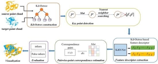
Training process: To compare and analyze the performance of 3DSmoothNet, D3Feat, and SpinNet, this section describes their training processes in detail.

3DSmoothNet [11] has adopted the nearest neighboring algorithm to search the matching points, where the searching radius has been set to 0.1. Then, the accuracy is calculated as

$$accuracy=\sum _{i=1}^K(P_i/K)$$

(1)

where K is the total num of points and $P_i$ is the number of neighboring points that match the i-th key point. In our experiments, the training dataset we have used is BundleFusion [49], which is a subset of 3DMatch and includes 19 files with a size of 51.7 GB.

Instead of performing a neighboring search, D3Feat [10] first computes the difference between the furthest positive sample and the closest negative sample, and then counts the number of points where the difference is less than 0. Suppose ($A_i$, $B_i$) is a corresponding pair and the two points have their corresponding descriptors, $D_{\alpha ,p}\left(i\right)={∥d_{A_i}-d_{B_i}∥}_2$, whereas the distance between a negative pair is $D_{\alpha ,n}\left(i\right)=min\left\{{∥d_{A_i}-d_{B_i}∥}_2\right\}{s}_{·}{t}_{·}{∥B_j-B_i∥}_2>R$, where R is the safe radius and $B_j$ is the hardest negative sample that lies outside the safe radius of the true correspondences. Based on these basic definitions, the furthest positive and the closest negative refers to the maximum value of $D_{a,p}$ and the minimum value of $D_{a,n}$, respectively. The accuracy is computed as

$$accuracy=(\sum _{i=1}^K{\mathrm{\Omega }}_{max\left(D_{a,p}\left(i\right)\right)}\le \underset{min\left(D_{a,n}\left(i\right)\right)}{min})/K$$

(2)

where $\mathrm{\Omega }$ is the number of key points wherein $D_{a,p}\left(i\right)$ is less than $D_{a,n}\left(i\right)$ and K is the number of key points. However, the network model suffers from network collapse issues during the training process owing to the loss function. According to Figure 5, the network collapses at epoch of 140, which is caused by the inherent defect of the unsupervised contrastive loss function [50]. We have replicated the network repeatedly and the resultant maximum training accuracy is 47.13%. We have adopted the model with the best training effect to extract the descriptor feature for each point, and the final feature recall is 90.33%, as listed in Table 3. Taking the training process and experimental results, we strongly argue that such high feature matching recall of D3Feat should be attributed to the dense feature descriptor instead of the network structure itself.

Thereafter, SpinNet [9] has also adopted Formula (2) to compute the accuracy, where the number of key points is identical to the value of the batch size with the default value of 76. We have reset that to 14 owing to the high computational and memory cost. Following SpinNet, the training dataset we have used is SUN3D [51] and 7-Scenes [52], besides the two subsets of 3DMatch. This includes a total of 19 files, and the size is 34.7 GB. According to Formula (2), we assume that the anchor point and the positive point will be matched when the distance of each of the valid anchor positive pair is less than that of the anchor negative pair. The experimental results show that the training process is instable, with large up and down fluctuations falling in the range of [35.7%, 100%]. For a comparison, we have adopted the same computing method of the training accuracy with 3DSmoothNet to re-train SpinNet. The training runs 50,424 steps, whereas other parameter settings are kept the same as in the previous experiments. The average training accuracies of the two epochs are 71.43% and 82.38%, respectively.

Learning rate: For the setting of the learning rate, the current practice is to use a dynamic strategy to adjust the learning rate during the training process. For example, 3DSmoothNet [11] and D3Feat [10] have adopted the exponential decay method to dynamically set the learning rate, as in Formula (3). For 3DSmoothNet network, the learning_rate, decay_rate, and decay_step values are 0.001, 0.95, and 5000, respectively. Nevertheless, SpinNet has employed another exponential decay method to adjust the learning rate, as given in Formula (4), which implies that the learning rate has changed once per epoch ($\gamma$ = 0.5).

$$decayed\_learning\_rate=learning\_rate\ast decay\_rat{e}^{global\_step/decay\_step}$$

(3)

$$new\_learning\_rate=learning\_rate\ast {\gamma }^{epoch}$$

(4)

Loss function: For the design of the loss functions, 3DSmoothNet [11] intends to minimize the soft margin batch hard loss during the training. D3Feat [10] has utilized the ordinary contrastive loss [50], as the contrastive learning is popular in Siamese networks and they have been experimentally found to give better convergence performance. Following D3Feat, SpinNet [9] has adopted the existing contrastive loss for end-to-end optimization. However, there exists a uniformity–tolerance dilemma in the contrastive learning, which is a problem not addressed to date. To further explore the effect of the loss functions on the 3D point cloud registration, we first formulate the three loss functions and perform certain experiments with the same network architecture to compare their effectiveness and efficiency. The loss functions are triplet loss, batch hard loss, and soft margin batch hard loss, in which batch hard loss is the improvement of triplet loss, and soft margin batch hard loss is a special case of batch hard loss.

Triplet loss, proposed by FaceNet [53], is a favored method for training the Siamese network. This loss function includes an anchor point $x^a$, a positive point $x^p$, and a negative point $x^n$. When these three points are input into a Siamese network to extract the features, we can obtain their corresponding feature vectors $f_{\theta }\left(x^a\right)$, $f_{\theta }\left(x^p\right)$, and $f_{\theta }\left(x^n\right)$, where $f_{\theta }$ is a function parameterized by $\theta$, which can be anything ranging from a linear transformation to non-linear mappings. Based on the three feature vectors, we can calculate the distance $D_{a,p}$ between the vectors $f_{\theta }\left(x^a\right)$ and the $f_{\theta }\left(x^p\right)$, and the distance $D_{a,n}$ between the vectors $f_{\theta }\left(x^a\right)$ and the $f_{\theta }\left(x^n\right)$. Following the training, a neural network should have the property that the feature vectors of the same category are clustered together, whereas the feature vectors of different categories are clearly separated. As shown in Figure 1, in the feature space, $D_{a,n}$ should be much larger than $D_{a,p}$, by a minimum margin m. If $D_{a,n}$≫$D_{a,p}$ + m, then there is no loss. Otherwise, the loss should be $D_{a,p}+m-D_{a,n}$. Hence, the triplet loss is defined as

$$\begin{array}{cc}\hfill L_{trip}(\theta ,x)& =max(0,{\displaystyle \frac{1}{\left|x\right|}}\sum _{a,p,n,y_a=y_p\ne y_n}[m+D_{a,p}-D_{a,n}])\hfill \\ \hfill D_{a,p}& =\parallel f_{\theta }\left(x^p\right)-f_{\theta }\left(x^a\right){\parallel }_2\hfill \\ \hfill D_{a,n}& =\parallel f_{\theta }\left(x^a\right)-f_{\theta }\left(x^n\right){\parallel }_2\hfill \end{array}$$

(5)

where $y_a$, $y_p$, and $y_n$ indicate the type to which the anchor point, positive sample, and negative sample belong, and indicates a mini-batch.

Batch Hard (BH) loss function [54] is a variant of triplet loss. The objective of the training is to make the distance between a positive sample and an anchor point to the minimum, whereas the distance between a negative sample and an anchor point should be the maximum. Hence, for each sample in a batch, Hermans et al. [54] selected the furthest positive and the closest negative samples within the batch while forming the triplets for computing the loss, which is called Batch Hard.

$$\begin{array}{c}\hfill L_{BH}(\theta ;x)={\displaystyle \frac{1}{x}}\sum _{i,j=1}^x[m+\stackrel{furthestpoisitive}{\overbrace{maxD(f_{\theta }\left(x_i^a\right),f_{\theta }\left(x_i^p\right))}}-\stackrel{closestnegative}{\overbrace{{min}_{j\ne i}D(f_{\theta }\left(x_i^a\right),f_{\theta }\left(x_i^n\right))}}]\end{array}$$

(6)

Soft Margin Batch Hard (SMBH) is the soft margin version of BH. SMBH replaces the hinge $loss[m+•]$ in Formula (6) by a smooth approximation using the soft-plus function, $ln(1+exp(•\left)\right)$, as the $log$ function generally produces stable implementations. Compared with BH, SMBH decays exponentially instead of having a cut-off, and it is referred as the soft margin loss function, defined as

$$\begin{array}{cc}\hfill L_{SMBH}(\theta ;x)& ={\displaystyle \frac{1}{x}}\sum _{i,j=1}^{x}ln(1+exp[\underset{i=i,\dots ,x}{max}{D}_{a,p}\hfill \\ \hfill & -\underset{j=1,\dots ,x,j\ne i}{min}{D}_{a,n}\left]\right)\hfill \\ \hfill & ={\displaystyle \frac{1}{x}}\sum _{i,j=1}^{x}ln(1+exp[\underset{i=i,\dots ,x}{max}{\parallel f_{\theta }\left(x_i^a\right)-f_{\theta }\left(x_i^p\right)\parallel }_2\hfill \\ \hfill & -\underset{j=1,\dots ,x,j\ne i}{min}\parallel f_{\theta }\left(x_i^a\right)-f_{\theta }\left(x_i^n\right){\parallel }_2\left]\right)\hfill \end{array}$$

(7)

3. Our Approach

Our end-to-end workflow is as follows. (i) We build a Kd–Octree to organize the massive point clouds and represent the input points as voxel grids in the leaf nodes of Kd–Octree, centered on the interest points and aligned with the Local Reference Frame (LRF). (ii) We feed the Kd–Octree based voxel grids to our KdO-Net to produce the unit length feature descriptors. (iii) We establish the pairwise-point correspondence by applying mutually nearest neighbor search in feature space, and (iv) match the pairwise point cloud fragments in an iterative fashion, evaluate the performance of our KdO-Net for the correspondence search on the indoor and outdoor real-world point cloud datasets, and visualize the final point cloud matching result of the two fragments, as shown in Figure 2.

3.1. Kd–Octree Based Voxelization Descriptor

3.1.1. Kd–Octree Construction

In our previous work on ground point filtering based on the vehicle LiDAR point cloud, a hybrid index structure combining the global Kd-tree and local octree, called Kd–OcTree index [55], has been proposed to improve the efficiency of the data organization and management. We construct a similar spatial index structure to speed up the nearest neighbor search, though with a different corresponding point search strategy, and generalize across multiple sensor modalities (from vehicle to terrestrial laser scanners) and from outdoor to indoor scenes.

Logical structure of Kd–Octree. While constructing the global Kd tree, each layer node is divided on a dimension $D_i$ ($i=x,y,z$) determined by the current layer discriminator, and the median of all points on the current Di is taken as the segmentation plane. To improve the efficiency of the overall Kd tree construction, the threshold of the number of points on Kd tree leaf nodes is set to 80,000, and when the number of points included in the node is less than this threshold, the division of the current node is terminated and this node is marked as a leaf node. In the 3DMatch dataset, the constructed global Kd tree consists of three layers, which are divided by the x, y, and z axes.

To save the storage space, the real point clouds are stored in the leaf nodes directly, instead of the root and intermediate nodes of the global Kd tree. This storage method compresses the amount of data storage and enables a fast retrieval by quickly locating each leaf node from the root node according to the pointers. Each leaf node of the Kd tree is reorganized according to the data organization of an octree. The construction of the entire hybrid index is complete after the construction of the local octrees in all leaf nodes in the Kd tree.

Data structure of the Kd–Octree: The data structure of the Kd–Octree hybrid index consists of five data objects, of which KdTree represents a Kd tree structure type, and KdNode is a Kd tree node structure type, Stack is a stack structure type, LinkStack a chain stack structure type, and Octree an octree type. Unlike the recursive method and fixed-length array data structure generally employed to construct the index structure, this work constructs the stack data structure in a cyclic way. The stack data structure is a dynamic allocation storage method, which allocates the maximum storage for use and releases the storage space immediately after the data leaves the stack. The memory occupation rate is greatly reduced by storing only the pointers to the nodes in the stack while building the Kd–Octree hybrid index, instead of the real point cloud.

The advantage of Kd–Octree is twofold. Global Kd-tree reconstructs the spatial neighborhood relations through defining the segmenting dimension and segmenting planes, which ensures the balance of the whole index. Then the local octree is constructed in the leaves of the Kd tree, which can avoid certain shortcomings, such as the imbalance of the point clouds distribution, deeper octree, and large amount of non-point space. The results show that the Kd–Octree index can speed the neighborhood searching (Section 4.1) and improve the efficiency of feature matching (Section 5.2).

3.1.2. Nearest Neighbor Searching Strategy

The search starts from the first node of the query and obtains the point cloud information stored in the corresponding node. When the leaf nodes satisfy the nearest neighbor condition, a hierarchical traversal is applied, and the search strategy employed for each node to be checked is depicted in Algorithm 1.

Algorithm 1: Nearest Neighbor Searching Strategy

0: kdtree.push(root) 1: while$kdq$ is not null do 2:   top=$kdq$.pop() 3:   if top->lchild != null and top->rchild != null then 4:     if abs(top->$kd\_cuttingCoordinate$[top->$kd\_cuttingDim$] -     $query\_point$[top-$>kd\_cuttingDim$]) <= R then 5:       $kdq$.push(top->lchild) 6:       $kdq$.push(top->rchild) 7:     else 8:       if $query\_point$[top->$kd\_cuttingDim$]<=       top->$kd\_cuttingCoordinate$[top->$kd\_cuttingDim$] then 9:         $kdq$.push(top->lchild) 10:       else 11:         $kdq$.push(top->rchild) 12:       end if 13:     end if 14:   else 15:     $resq$.push(top->thisOctree) 16:   end if 17: end while

In Algorithm 1, kdq represents the Kd tree queue, which stores the number of Kd tree nodes traversed, whereas resq represents the octree node queue, which stores the final searched octree leaf node information. R is the radius of nearest neighbor search and query_point is the key point, i.e., the one to search its neighboring points. kd_cuttingCoordinate indicates the splitting coordinates, whereas kd_cuttingDim indicates the splitting dimension. While performing a neighborhood search, we use the absolute value of the difference between the corresponding point and the key point in the current splitting dimension to represent the distance between them. If this distance is less than the searching radius R, then the neighborhood search is performed in the left and right subtrees in a hierarchical traversal manner. Otherwise, it is sufficient to search in only one branch.

Unlike 3DSmoothNet, which encodes the unstructured 3D point clouds as the SDV grids directly, our method first constructs a Kd–Octree data structure, computes the LRF around interest points in the leaf nodes of Kd–Octree with the hierarchical traversal strategy, and then produces the point cloud patches that transform them into SDV voxel grids and feed them to the network.

3.2. Feature Descriptor Extraction

3.2.1. KdO-Net Architecture

Figure 2 shows the network architecture of our KdO-Net which learns to distinguish between the matching pairs with a two-branch Siamese architecture [24,27,56,57]. Inspired by (but different from) 3DSmoothNet, (i) we built upon the Kd–Octree representation, and our network takes Kd–Octree based voxelized patches computed at the leaf nodes as input. Further, (ii) our network includes two basic modules in each branch, viz., Extender and Compressor, as shown in Figure 3. The Extender is employed to preserve the rich local geometric information when the resolution of point clouds is reduced during training, whereas the Compressor aims to obtain a smaller descriptor to reduce the computational cost and speed up the feature extraction without compromising the performance. Hence, KdO-Net architecture is a simple yet effective network which consists of 12 convolutional layers. The first 11 convolutional layers are followed by the batch normalization and the ReLu activation function, whereas the last convolutional layer is followed by $l_2$-normalization to normalize the output. KdO-Net applies the stride of 2 in the 4th layer and valid padding in the 11th and 12th layers (instead of pooling) to down-sample the voxel grid.

According to the above description, we find that KdO-Net architecture is a well-structured, simple, and straightforward network. Extensive experimental results in Section 4.3 and Section 5 will demonstrate the feasibility, effectivity, and practicality of our network.

3.2.2. Network Training

Considering the SGDR learning rate, to tackle the problem of the fast dropping of exponential decay, according to Figure 4a, we have adopted a warm restart technique, viz., Stochastic Gradient Descent with Warm Restarts (SGDR) [58], to adjust the learning rate, which is common in gradient-free optimization. Further, it gradually becomes popular in the gradient-based optimization to avoid being trapped in a local optimum and speed up convergence. We employ cosine decay restarts, where we only simulate a warm restart once another epoch is performed, as given below

$$decayed\_lr=l{r}_{min}^i+{\displaystyle \frac{1}{2}}(l{r}_{max}^i-l{r}_{min}^i)(1+cos\left({\displaystyle \frac{T_{cur}}{T_i}}\pi \right))$$

(8)

where $l{r}_{min}^i$ and $l{r}_{max}^i$ are the range for the learning rate, $T_i$ the number of epochs, $T_{cur}$ the number of epochs that have been performed since the last restart, and i the index of iteration. The restart implies that the learning rate is updated to the initial value, by not performing the training from scratch. Figure 4b demonstrates the adjustment of the learning rate with cosine decay restarts.

Huber and Cross Entropy loss. Based on the mathematical analysis and experimental results of triplet loss, batch hard loss, and soft margin batch hard loss, introduced in Section 2.2, the calculation of loss in [11] employs the result of the difference between the furthest positive points ($D_{a,p}$) and the closest negative points ($D_{a,n}$). To highlight the difference between $D_{a,p}$ and $D_{a,n}$ for minimizing, $D_{a,p}$ and $-D_{a,n}$ are set to be non-linearized to enhance the descriptiveness of the network model. Our calculation is shown below

$$\begin{array}{cc}\hfill L_{HCE}& =(\underset{i=1,\dots ,x}{max}{D}_{a,p}+\underset{j=1,\dots ,x,j\ne i}{min}(-D_{a,n}))/2\hfill \\ \hfill D_{a,p}& ={\displaystyle \frac{1}{x}}\sum _{i=1}^x{(f_{\theta }(x_i^a)-f_{\theta }(x_i^p))}^2\hfill \\ \hfill -D_{a,p}& ={\displaystyle \frac{1}{x}}\sum _{i,j=1;j\ne i}^{x}ln(1+e^{-|f_{\theta }\left(x_i^a\right)-f_{\theta }(x_i^n)|})\hfill \end{array}$$

(9)

where the Huber loss function is applied to compute the loss of the furthest positive points and the Cross Entropy is used for the closest negative points. Therefore, this loss algorithm is termed as Huber and Cross Entropy (HCE) loss function in this work.

3.3. Pairwise-Point Correspondence Establishment

For each pair of corresponding fragments S and T, we establish the correspondence by the following steps. First, we find the mutually closest point pairs in feature space based on the source descriptor and target descriptor obtained from our KdO-Net model. Then, we search the ground truth transformation matrix to make sure whether there is the transformation matrix $Ma{t}_{s\_t}$ between S and T. If it exists, the $Ma{t}_{s\_t}$ can be obtained directly, otherwise the transformation matrix between the two is calculated indirectly in a circular fashion. For example, if the transformation matrix $Ma{t}_{s\_p}$ between S and P and the transformation matrix $Ma{t}_{p\_t}$ between P and T are known, then the transformation matrix between S and T can be derived by performing matrix multiplication

$$Ma{t}_{s\_t}^{{}^{\prime }}=Ma{t}_{s\_p}\ast Ma{t}_{p\_t},$$

(10)

where $Ma{t}_{s\_t}^{{}^{\prime }}$ represents a complement to $Ma{t}_{s\_t}$. Next, the source point cloud P and the target point cloud Q, belonging to the two fragments S and T, respectively, are converted to the same coordinate system by applying the transformation matrix $Ma{t}_{s\_t}$, i.e., we transform the target point cloud to the coordinate system of source point cloud

$$Q_i^{{}^{\prime }}=Ma{t}_{s\_t}\ast Q_i,$$

(11)

where $Q_i^{{}^{\prime }}$ is the target point cloud after transformation. Thus far, we have obtained the corresponding pairs ($P_i$,$Q_i^{{}^{\prime }}$) between the two fragments S and T.

3.4. Pairwise-Point Feature Matching

Suppose two points have their corresponding descriptors $d_{P_i}$ and $d_{Q_i}^{{}^{\prime }}$. The distance between the correspondence pair is defined as the Euclidean distance between their descriptors as follows

$$di{s}_i=\parallel d_{P_i}-d_{Q_i}^{{}^{\prime }}{)\parallel }_2.$$

(12)

Following the setting of [12], the correspondence are seen as inliers when the distance $di{s}_i$ is less than the inlier distance threshold ${\tau }_1$ = 10 cm. The fragment pairs which have more than ${\tau }_2$ = 5% inlier correspondences will be counted as one match, where ${\tau }_2$ is the inlier ratio threshold. It should be noted that the match obtained with $Ma{t}_{s\_t}$ is correct feature matching, while the match obtained with $Ma{t}_{s\_t}$ denotes the correct match that would have been skipped if based only on the $Ma{t}_{s\_t}$. According the feature matching metrics introduced in Section 4.2.2, we can evaluate the efficiency and robustness of our approach, with specific validation results presented in Section 4.3.

4. Results

Our approach is implemented in Python using TensorFlow, including the feature descriptor extraction and feature matching of point clouds between every two fragments. Our network is only trained with the BundleFusion [49], a small part of indoor 3DMatch [12]. Further, we evaluate its generalization on the challenging outdoor ETH [59] and apply it to our own TUM-lab dataset. Lastly, we have conducted an extensive ablation experiment on BundleFusion to study the efficiency of each component of KdO-Net.

4.1. Implementation

Owing to the unstructured and sparse nature of 3D point cloud, it is crucial to adopt a reasonable representation of the data before feeding the network. Similar to [11], this paper encodes an unstructured raw point clouds as the structured SDV grids amenable to the convolutional layers of the standard deep learning libraries. Alternatively, this representation of SDV reduces the sparsity of the input voxel grid and reduces the boundary effects. Further, it smooths out small misalignments owing to the errors in the estimation of the LRF and improves the generalization ability of the network, as explained in the original paper [11]. For the size of SDV voxel grids, we use 0.3 m and 1 m for 3DMatch and ETH datasets, respectively, as the point clouds of ETH are sparser by comparing with 3DMatch.

To generate the training examples, we follow the methods of [9,10,11,12] to randomly sample 300 anchor points $p^a$ from more than 30% overlap of two fragments, $F_i$ and $F_j$. The positive example $p^p$ is the potential matching point that represents the nearest-neighbor $p^p=:nn\left(p^a\right)\in T_j\left(F_j\right)$, where nn() denotes the nearest neighbor search in the Euclidean space based on the l2 distance. Instead, the negative example $p^n$ is the non-matching point that has been sampled on the fly from all the positive examples of the mini-batch. How to distinguish the positive and negative points is a question. We define positive points as point clouds whose distance from the anchor point are below a threshold, $\mathrm{dis}(\mathrm{anchor},\mathrm{positive})<{\tau }_p$, whereas the negative points are point clouds whose distance from the anchor point are greater than a threshold, $dis\left(\mathrm{anchor},\mathrm{positive}\right)>{\tau }_n$ [24,26].

For a comparison, we keep the same setting for all the experiments and adopt the same algorithms and metrics to evaluate their performance. All experiments are conducted on the platform with Intel Xeon CPU @3.60 GHz and NVIDIA Quadro RTX 4000 GPU. During the training, we test different batch sizes, compare the efficiency of the descriptor learning and final feature matching performance with the metrics introduced in Section 4.2.2, and eventually use the batch size of 128 on BundleFusion to train our network KdO-Net. Despite the fact that the network with a batch size of 128 is not the best-performing model on the training and evaluation datasets, it keeps the consistency between the training effectiveness and the final feature matching performance. We then optimize the network using Adadelta optimizer with an initial learning rate of 1.0, and the cosine decay restarts adjustment strategy with 40,000 steps per epoch. The network needs only 80,000 steps and normally converges within 2 epochs.

4.2. Evaluation Metrics

4.2.1. Nearest Neighbor Searching and Network Training

For the corresponding search, the time complexity has been reduced to $O\left(NlogN\right)$ using the Kd–Octree based method, where N denotes the number of points. To evaluate the efficiency of the Kd–Octree based nearest neighbor searching, we perform the supplementary trial and compare with 3DSmoothNet [11] in terms of the average nearest neighbor searching time of per key point on BundleFusion training set in

Table 1. Average nearest neighbor searching time per interest point on each scene of BundleFusion training set (ms).

Model	Apt0	Apt1	Apt2	Copyroom	Office0	Office1	Office2	Office3	Avg
3DSmoothNet	1.09	1.01	1.24	0.94	1.08	1.11	1.06	1.07	1.07
KdO-Net	0.37	0.36	0.44	0.32	0.36	0.39	0.36	0.37	0.37

, and the comparison on 3DMatch test set is presented in

Table 2. Average nearest neighbor searching time per interest point on each scene of 3DMatch test set (ms).

Model	Kitchen	Home1	Home2	Hotel1	Hotel2	Hotel3	Study	MIT Lab	Avg
3DSmoothNet	0.99	1.12	1.04	1.31	1.26	1.30	1.70	1.58	1.29
KdO-Net	0.34	0.37	0.34	0.42	0.41	0.40	0.51	0.47	0.37

, while running on the same PC with Intel Xeon CPU E5-2620 and 16G RAM. On both datasets, the average nearest neighbor searching time of our method is significantly reduced, e.g., 0.37 ms vs. 1.29 ms, which is shorter by 70%.

Furthermore, the training accuracy is an efficient metric used to measure the learning ability of a network. It is a metric that decides the accuracy of a model prediction, compared to the ground truth. In our experiments, the accuracy is calculated by every 100 steps.

4.2.2. Feature Matching Metrics

The performance of the feature matching is quantitatively assessed using the following evaluation metrics, inlier ratio (IR), mean recall (mR), standard deviation of mR (STD_mR), mean precision (mPR), and standard deviation of mPR (STD_mPR). IR measures the fraction of the inlier correspondences, given as the input for a set of putative correspondences built in the descriptor space for two fragments [36]. Recall and precision are mutually exclusive and often used in conjunction to provide a more comprehensive assessment of the effectiveness of the feature matching. The mR is defined as

$$\begin{array}{cc}\hfill mR& ={\displaystyle \frac{1}{\left|F\right|}}\sum _{f=1}^{\left|F\right|}(IR>{\tau }_2)\hfill \\ \hfill IR& ={\displaystyle \frac{1}{|C_f|}}\sum _{i,j\in C}(\parallel p_i-T_f\left(q_j\right){\parallel }_2<{\tau }_1)\hfill \end{array}$$

(13)

where $\left|F\right|$ is the number of scenes and ${\tau }_2$ is a threshold on the inlier ratio. This implies that, if the inlier ratio of the two fragments is not greater than ${\tau }_2$, the two fragments cannot be matched. For the computing of IR, ${∥p_i-T_f\left(q_j\right)∥}_2$ denotes the $l_2$-normalization, $\left|C_f\right|$ the number of fragment pairs in a scene, ${\tau }_1$ the threshold on the Euclidean distance between the correspondence pair (i, j), and $T_f$ denotes the ground-truth transformation alignment of the fragment pair $f\in F$. For a pairwise matching, the matching recall refer to the percentage of the successful matching whose IR is above certain threshold (i.e., ${\tau }_2$ = 5%), which measures the matching quality [10,11,15]. Based on the IR, the STD_mR is computed as

$$STD\_mR=\sqrt{{\displaystyle \frac{1}{\left|F\right|-1}}\sum _{f=1}^{\left|F\right|}{(I{R}_f-\overline{IR})}^2}$$

(14)

Following [55], the mPR is defined as

$$\begin{array}{c}\hfill mPR=\frac{1}{\left|F\right|}\sum _{f=1}^{\left|F\right|}PR\\ \hfill PR=\frac{TP}{TP+FP}\end{array}$$

(15)

where TP and FP are the numbers of the true and false positives, respectively. Similar to STD_mR, the STD_mPR is calculated as

$$STD\_mPR=\sqrt{\frac{1}{\left|F\right|-1}\sum _{f=1}^{\left|F\right|}{\left(P{R}_f-\overline{PR}\right)}^2}$$

(16)

4.3. Evaluation

4.3.1. Evaluation on the Indoor 3DMatch Dataset

Dataset: 3DMatch benchmark [12] is an RGB-D reconstruction dataset consisting of 62 real-world indoor scenes, collected from SUN3D [51], 7-Scenes [52], RGB-D Scenes v2 [60], BundleFusion [49], and Analysis by Synthesis [61]. Zeng et al. [12] have converted these datasets into a unified file structure and format, with 54 scenes for training and 8 scenes for testing. The size of the total dataset is 145 GB (328 files altogether). In our implementation, only BundleFusion set is chosen as the training set, which includes 19 files that are collected from eight other indoor scenes. Concerning the testing, we adopt the test set from 3DMatch by following the set of [12].

Training: For producing the Kd–Octree based descriptors, we generate the training set from the original BundleFusion. Consider a pair of fragments S and T, chosen from the overlapping region. To generate the training samples, we randomly sample 300 anchor points $P^a$ from S, and then apply the ground truth transformation matrix $Mat$ to determine the corresponding points $P^c$ in T. Next, we perform the Kd–Octree based nearest neighbor searching of $P^c$ to find the positive samples $P^p$, where the searching radius r = 0.7 m. Finally, we combine $P^a$ and $P^p$ to obtain the sample pairs [$P^a$, $P^p$] for training.

Figure 5 presents the training accuracies and the feature matching results of different models on the BundleFusion dataset. We experimentally find that our KdO-Net model has achieved good training accuracy, and the maximum and average values are the highest, but there is a little fluctuation and less stability due to the smaller training set. The mR and PR have already reached 91.66% and 97.63% respectively.

To explore the influence of different batch sizes on model training, we adjust the batch size from 16, 32, 64, and 128 to 256, and the corresponding feature matching results of KdO-Net are presented in Figure 6, which shows the performance of our network on 3DMatch test set is only a marginal improvement when we increase the batch size, whilst the precision is gradually decreasing. We find that the model is most stable when the batch size is equal to 128, and a trade-off between recall and precision is achieved.

For a comparison, the detailed experimental results of different models on the BundleFusion benchmark are summarized in

Table 3. Quantitative comparisons with the state-of-the-arts, training on BundleFusion and feature matching on 3DMatch test set. All results are reproduced on the same platform by ourselves. The best performance is shown in bold, and “–” denotes the value is unavailable.

Model	Convolution-Based Network				Feature Matching
	Batch Size	Training Accuracy	Validation Accuracy	Loss	mR	STD_mR	mPR	STD_mPR
3DSmoothNet	128	67.2	60.14	0.57	93.22	3.60	96.23	2.49
D3Feat(pred)	1	47.13	40.1	1.18	90.33	5.71	94.25	4.03
SpinNet	14	74.48	–	1.29	86.2	5.92	97.25	1.30
KdO-Net	128	78.4	63.08	0.49	91.66	5.46	97.63	1.30

, which involves the network evaluation and feature matching evaluation with the metrics introduced in Section 4.2.2. These are the maximal training and validation accuracy (in percent), the minimal loss, mR, STD_mR, mPR, and STD_mPR in percent. The experimental results show that our KdO-Net outperforms the alternative approach by a significant margin in terms of the network training. The detailed quantitative results of the precision of the different methods on each scene of the 3DMatch benchmark are listed in

Table 4. Precision (%) of different reproduced models on each scene of BundleFusion, a subset of 3DMatch, with ${\tau }_1$ = 10 cm and ${\tau }_2$ = 0.05. The best performance is shown in bold.

Scene	3DSmoothNet	D3Feat(pred)	SpinNet	KdO-Net
Kitchen	96.99	97.56	97.49	97.34
Home1	96.77	93.24	96.53	96.67
Home2	95.36	93.57	96.02	96.2
Hotel1	98.19	97.26	99.05	98.63
Hotel2	98.94	98.91	98.91	98.96
Hotel3	98.15	96.23	98.11	100
Study	94.77	91.67	95.14	96.51
MIT Lab	90.67	85.54	96.77	96.77
mPR	96.23	94.25	97.25	97.63
STD_mPR	2.49	4.03	1.30	1.30

, which shows that our KdO-Net outperforms all the state-of-the-art feature matching networks for most of the scenes.

Additionally, we demonstrate how precise feature matching can be obtained with our KdO-Net model under different inlier ratios (${\tau }_2$) and inlier distance (${\tau }_1$) threshold (originally ${\tau }_2$ = 0.05 and ${\tau }_1$ = 10 cm). As shown in Figure 7, the descriptor learned with our KdO-Net outperforms all other models under different thresholds. More importantly, our model still outperforms other methods even with a strict inlier ratio threshold (e.g., ${\tau }_2$ = 0.2). With the increase in the inlier distance threshold, the precision inevitably decreases. The precision of our model achieves 91%, while 3DSmoothNet, SpinNet, and D3Feat drop to 89.6%, 89.1%, and 88.1%, respectively.

4.3.2. Generalization from BundleFusion to ETH Dataset

To evaluate the generalization ability of our proposed KdO-Net, we have conducted a series of experiments on four outdoor laser scanner datasets, viz., Gazebo-Summer, Gazebo-Winner, Wood-Summer, and Wood-Autumn, from the ETH dataset (Pomerleau et al., 2012), with the model trained on BundleFusion. We have followed the protocols defined in (Gojcic et al., 2019), where the voxel size equals 6.25 cm (16 voxels per 1 m, corresponding to 16 voxels per 0.3 m on the 3DMatch dataset) owing to the lower resolution of the point clouds in the ETH dataset. According to

Table 5. Quantitative results on ETH dataset at ${\tau }_1$ = 10 cm, ${\tau }_2$ = 5%, and $size\_of\_voxel\_grid$ = 1 m are compared.

Model	Gazebo		Wood		mR	STD_mR	mPR
	Summer	Winter	Summer	Winter
3DSmoothNet	82.61	64.36	57.39	63.2	66.89	9.45	100
KdO-Net	84.24	70.93	62.61	68.0	71.45	7.96	100

, our KdO-Net outperforms 3DSmoothNet on all scenes with the Kd–Octree based descriptors.

5. Discussion

5.1. Application

To evaluate the efficiency and practicality of our KdO-Net, we apply it to a substantial point cloud registration task. Our test scenery shows a laboratory in the basement of the Chair of Geodesy, Technical University of Munich, partly used as a storage facility, containing different geodetic measurement equipment and facilities, old technical equipment such as an industrial robot, and stored furniture. The measured room has an approximate dimension of 18.2 m ∗ 11.5 m ∗ 2.3 m.

The dataset consists of three sites of point cloud, captured with a terrestrial laser scanner Leica RTC360 from three different stations. The three point clouds are registered precisely with the manufacturers’ software Cyclone. Following the registration, the point clouds are subsampled to a mean point spacing of 4mm to be comparable with the 3DMatch dataset. To generate a higher number of fragments, the registered point cloud of each station is partitioned into 16 parts, depending on its horizontal angle. These sub-fragments are cyclically composed to sets of four, forming the 15 final point cloud fragments with an approximate overlap between 75% and 15%. The coordinates corresponding to each fragment are transformed by the inverse of the randomly generated homogeneous transformation matrix. The resulting fragments contain between 1.5 and 4.4 million individual points, depending on the objects in the scenery.

We evaluate our approach through extensive applications and visual interpretations, shown in Figure 8. The left column represents two fragments before registration, and the right column shows the corresponding registration results. The overlapping area of the first row is 31.5%, whereas the overlapping area of the second and third rows is only 17.6% and 11.2%, respectively. To quantitatively evaluate the alignment accuracy, we employ the root mean square error (RMSE) of the distance between a point cloud and its reference point cloud as a measure. When RMSE is below 0.2 m, it indicates that the final performance for the practical use is good [10]. Following [11,12], we use the RANSAC algorithm to estimate the rigid transformation between the two point clouds, and then calculate the RMSE of the ground truth correspondence under the estimated transformation [10]. The RMSE of the three examples is 3.28 cm, 3.36 cm, and 3.31 cm, which further demonstrate that the feature descriptors extracted with our network are discriminative and powerful, even for challenging tasks.

5.2. Ablation Study

In this section, we conduct extensive ablation studies on BundleFusion dataset to systematically evaluate the effectiveness of the separate components in our KdO-Net, including the SGDR learning rate, HCE loss function, compressor module, network architecture, and Kd–Octree.

Table 6. The score of network training and feature matching of all ablated experiments on the Bundlefusion dataset (a subset of 3DMatch) at ${\tau }_1$ = 10 cm and ${\tau }_2$ = 0.05.

Component	Training Accuracy	Loss	mR	mPR
w/o SGDR	10.96	0.50	3.89	-
w/o HCE	71.89	−0.26	94.07	95.61
w/o compressor	73.05	−0.26	90.53	97.40
simplify SCS-Net	67.06	0.50	87.28	97.50
w/o Kd–Octree	71.09	0.49	89.82	97.63
the full method	78.4	0.49	90.23	97.74

demonstrates the experimental results.

Replacing SGDR learning rate with exponential decay: Instead of adopting the cosine decay restarts strategy, we employ a commonly used exponential decay method to adjust the learning rate. The initial learning rate is 0.001, and the rate of exponential learning rate decaying is 0.95. The training step is 80,000, and the frequency of exponential learning rate decaying is 20. The results show that the training accuracy drops to 10.96%, which implies that the network cannot converge. Consequently, the average feature matching recall is as low as 3.89.

Replacing HCE loss with BH loss: For the pairwise point feature matching, the key is to highlight the difference between the furthest positive points and the closest negative points to minimize the loss. To validate the effectiveness of our proposed HCE loss function, we have replaced it with the popular batch hard loss. Our method brings a significant improvement in the precision.

Remove the Compressor: To evaluate the function of the Compressor, we have removed it directly and concatenated the last layer of the Extender with the output layer. We find that the precision decreases, though the training accuracy and mean recall increase owing to the sparsity of the point clouds on BundleFusion.

Simplify KdO-Net architecture with a Siamese Network: To evaluate the efficiency of our network structure, we have replaced it with a simplified Siamese network, which includes five convolutional layers and the channel list [1, 32, 64, 128, 64, 32, 32]. We remove the convolutional blocks with the same channel in the Encoder component and replace them with an individual convolutional layer. According to Table 6, the learning performance of the network drops to 11%, and the mean feature matching recall and average precision drop by 2.95% and 0.24%, respectively. If a MLP is used directly, there would be a sharp decrease in the learning effect.

Remove Kd–Octree data structure: To evaluate the effect of Kd–Octree on the point cloud feature matching, we have removed the data structure directly and produced the descriptor with the original method. The experimental results demonstrate that the effect of the feature matching has been reduced.

6. Conclusions

We propose a Kd–Octree based convolutional network, KdO-Net, which takes the advantages of the global Kd-tree and local Octree to enable the balance of the data structure and fast computation. We have found that, experimentally, this hybrid index achieves better performance in the search for the nearest neighbors, and the ablation experiments have proven that it also facilitates the final effect of the feature matching. KdO-Net includes two modules, viz., Extender and Compressor. Further, it incorporates Huber and Cross Entropy loss, connecting the adjustment strategy of Stochastic Gradient Descent with a warm Restart, to ensure that our network can converge in the correct direction. Besides training on BundleFusion and generalizing to ETH, we also validate the efficiency and practicality by using the TUM-lab dataset, captured in the cluttered indoor scenes with an overlap of 15% using a terrestrial laser scanner. We expect that KdO-Net will stimulate more on the learning-based point feature matching. Future research includes the optimization of the data structure and designing the adaptive network to learn the 3D descriptors.

References

1. Huang, R.; Ye, Z.; Boerner, R.; Yao, W.; Xu, Y.; Stilla, U. Fast pairwise coarse registration between point clouds of construction sites using 2D projection based phase correlation. Int. Arch. Photogramm. Remote Sens. Spat. Inf. Sci. 2019, 42, 1015–1020. [Google Scholar] [CrossRef] [Green Version]
2. Dong, Z.; Yang, B.; Liang, F.; Huang, R.; Scherer, S. Hierarchical registration of unordered TLS point clouds based on binary shape context descriptor. ISPRS J. Photogramm. Remote Sens. 2018, 144, 61–79. [Google Scholar] [CrossRef]
3. Montuori, A.; Luzi, G.; Stramondo, S.; Casula, G.; Bignami, C.; Bonali, E.; Bianchi, M.G.; Crosetto, M. Combined use of ground-based systems for Cultural Heritage conservation monitoring. In Proceedings of the 2014 IEEE Geoscience and Remote Sensing Symposium, Quebec City, QC, Canada, 13–18 July 2014; IEEE: Piscataway, NJ, USA, 2014; pp. 4086–4089. [Google Scholar]
4. Davis, A.; Belton, D.; Helmholz, P.; Bourke, P.; McDonald, J. Pilbara rock art: Laser scanning, photogrammetry and 3D photographic reconstruction as heritage management tools. Herit. Sci. 2017, 5, 25. [Google Scholar] [CrossRef] [Green Version]
5. Dong, Z.; Liang, F.; Yang, B.; Xu, Y.; Zang, Y.; Li, J.; Wang, Y.; Dai, W.; Fan, H.; Hyyppä, J. Registration of large-scale terrestrial laser scanner point clouds: A review and benchmark. ISPRS J. Photogramm. Remote Sens. 2020, 163, 327–342. [Google Scholar] [CrossRef]
6. Xu, Y.; Boerner, R.; Yao, W.; Hoegner, L.; Uwe, S. Pairwise coarse registration of point clouds in urban scenes using voxel-based 4-planes congruent sets. ISPRS J. Photogramm. Remote Sens. 2019, 151, 106–123. [Google Scholar] [CrossRef]
7. Guo, Y.; Sohel, F.; Bennamoun, M.; Wan, J.; Lu, M. An Accurate and Robust Range Image Registration Algorithm for 3D Object Modeling. IEEE Trans. Multimed. 2014, 16, 1377–1390. [Google Scholar] [CrossRef]
8. Zhu, X.X.; Tuia, D.; Mou, L.; Xia, G.S.; Zhang, L.; Xu, F.; Fraundorfer, F. Deep learning in remote sensing: A comprehensive review and list of resources. IEEE Geosci. Remote Sens. Mag. 2017, 5, 8–36. [Google Scholar] [CrossRef] [Green Version]
9. Ao, S.; Hu, Q.; Yang, B.; Markham, A.; Guo, Y. SpinNet: Learning a General Surface Descriptor for 3D Point Cloud Registration. In Proceedings of the IEEE/CVF Conference on Computer Vision and Pattern Recognition, Nashville, TN, USA, 20–25 June 2021; pp. 11753–11762. [Google Scholar]
10. Bai, X.; Luo, Z.; Zhou, L.; Fu, H.; Quan, L.; Tai, C.L. D3feat: Joint learning of dense detection and description of 3d local features. In Proceedings of the IEEE/CVF Conference on Computer Vision and Pattern Recognition, Seattle, WA, USA, 13–19 June 2020; pp. 6359–6367. [Google Scholar]
11. Gojcic, Z.; Zhou, C.; Wegner, J.D.; Wieser, A. The perfect match: 3d point cloud matching with smoothed densities. In Proceedings of the IEEE/CVF Conference on Computer Vision and Pattern Recognition, Long Beach, CA, USA, 15–20 June 2019; pp. 5545–5554. [Google Scholar]
12. Zeng, A.; Song, S.; Nießner, M.; Fisher, M.; Xiao, J.; Funkhouser, T. 3dmatch: Learning local geometric descriptors from rgb-d reconstructions. In Proceedings of the IEEE Conference on Computer Vision and Pattern Recognition, Honolulu, HI, USA, 21–26 July 2017; pp. 1802–1811. [Google Scholar]
13. Aoki, Y.; Goforth, H.; Srivatsan, R.A.; Lucey, S. Pointnetlk: Robust & efficient point cloud registration using pointnet. In Proceedings of the IEEE/CVF Conference on Computer Vision and Pattern Recognition, Long Beach, CA, USA, 15–20 June 2019; pp. 7163–7172. [Google Scholar]
14. Fang, Y.; Xie, J.; Dai, G.; Wang, M.; Zhu, F.; Xu, T.; Wong, E. 3d deep shape descriptor. In Proceedings of the IEEE Conference on Computer Vision and Pattern Recognition, Boston, MA, USA, 7–12 June 2015; pp. 2319–2328. [Google Scholar]
15. Deng, H.; Birdal, T.; Ilic, S. Ppf-foldnet: Unsupervised learning of rotation invariant 3d local descriptors. In Proceedings of the European Conference on Computer Vision (ECCV), Munich, Germany, 8–14 September 2018; pp. 602–618. [Google Scholar]
16. Elbaz, G.; Avraham, T.; Fischer, A. 3D point cloud registration for localization using a deep neural network auto-encoder. In Proceedings of the IEEE Conference on Computer Vision and Pattern Recognition, Honolulu, HI, USA, 21–26 July 2017; pp. 4631–4640. [Google Scholar]
17. Deng, H.; Birdal, T.; Ilic, S. Ppfnet: Global context aware local features for robust 3d point matching. In Proceedings of the IEEE Conference on Computer Vision and Pattern Recognition, Salt Lake City, UT, USA, 18–22 June 2018; pp. 195–205. [Google Scholar]
18. Poiesi, F.; Boscaini, D. Generalisable and distinctive 3D local deep descriptors for point cloud registration. arXiv 2021, arXiv:2105.10382. [Google Scholar]
19. Wang, Y.; Solomon, J.M. Deep closest point: Learning representations for point cloud registration. In Proceedings of the IEEE/CVF International Conference on Computer Vision, Seoul, Korea, 27 October–2 November 2019; pp. 3523–3532. [Google Scholar]
20. Li, J.; Chen, B.; Yuan, M.; Zhao, Q.; Luo, L.; Gao, X. Matching Algorithm for 3D Point Cloud Recognition and Registration Based on Multi-Statistics Histogram Descriptors. Sensors 2022, 22, 417. [Google Scholar] [CrossRef]
21. Yue, X.; Liu, Z.; Zhu, J.; Gao, X.; Yang, B.; Tian, Y. Coarse-fine point cloud registration based on local point-pair features and the iterative closest point algorithm. Appl. Intell. 2022, 1–15. [Google Scholar] [CrossRef]
22. Sun, L.; Zhang, Z.; Zhong, R.; Chen, D.; Zhang, L.; Zhu, L.; Wang, Q.; Wangb, G.; Zou, J.; Wangc, Y. A Weakly Supervised Graph Deep Learning Framework for Point Cloud Registration. IEEE Trans. Geosci. Remote Sens. 2022, 60, 5702012. [Google Scholar] [CrossRef]
23. Hana, X.F.; Jin, J.S.; Xie, J.; Wang, M.J.; Jiang, W. A comprehensive review of 3D point cloud descriptors. arXiv 2018, arXiv:1802.02297. [Google Scholar]
24. Poiesi, F.; Boscaini, D. Distinctive 3D local deep descriptors. In Proceedings of the 2020 25th International Conference on Pattern Recognition (ICPR), Milan, Italy, 10–15 January 2021. [Google Scholar]
25. Spezialetti, R.; Salti, S.; Stefano, L.D. Learning an effective equivariant 3d descriptor without supervision. In Proceedings of the IEEE/CVF International Conference on Computer Vision, Seoul, Korea, 27 October–2 November 2019; pp. 6401–6410. [Google Scholar]
26. Tian, Y.; Fan, B.; Wu, F. L2-net: Deep learning of discriminative patch descriptor in euclidean space. In Proceedings of the IEEE Conference on Computer Vision and Pattern Recognition, Honolulu, HI, USA, 21–26 July 2017; pp. 661–669. [Google Scholar]
27. Yew, Z.J.; Lee, G.H. 3dfeat-net: Weakly supervised local 3d features for point cloud registration. In Proceedings of the European Conference on Computer Vision (ECCV), Munich, Germany, 8–14 September 2018; pp. 607–623. [Google Scholar]
28. Choy, C.; Dong, W.; Koltun, V. Deep global registration. In Proceedings of the IEEE/CVF Conference on Computer Vision and Pattern Recognition, Seattle, WA, USA, 14–19 June 2020; pp. 2514–2523. [Google Scholar]
29. Lu, W.; Wan, G.; Zhou, Y.; Fu, X.; Yuan, P.; Song, S. DeepICP: An end-to-end deep neural network for point cloud registration. In Proceedings of the IEEE/CVF International Conference on Computer Vision, Seoul, Korea, 27 October–2 November 2019; pp. 12–21. [Google Scholar]
30. Feng, M.; Hu, S.; Ang, M.H.; Lee, G.H. 2d3d-matchnet: Learning to match keypoints across 2d image and 3d point cloud. In Proceedings of the 2019 International Conference on Robotics and Automation (ICRA), Montreal, QC, Canada, 20–24 May 2019; IEEE: Piscataway, NJ, USA, 2019; pp. 4790–4796. [Google Scholar]
31. Lowe, D.G. Object recognition from local scale-invariant features. In Proceedings of the Seventh IEEE International Conference on Computer Vision, Kerkyra, Greece, 20–27 September 1999; IEEE: Piscataway, NJ, USA, 1999; Volume 2, pp. 1150–1157. [Google Scholar]
32. Zhong, Y. Intrinsic shape signatures: A shape descriptor for 3d object recognition. In Proceedings of the 2009 IEEE 12th International Conference on Computer Vision Workshops, ICCV Workshops, Kyoto, Japan, 27 September–4 October 2009; IEEE: Piscataway, NJ, USA; pp. 689–696. [Google Scholar]
33. Li, L.; Zhu, S.; Fu, H.; Tan, P.; Tai, C.L. End-to-end learning local multi-view descriptors for 3d point clouds. In Proceedings of the IEEE/CVF Conference on Computer Vision and Pattern Recognition, Seattle, WA, USA, 13–19 June 2020; pp. 1919–1928. [Google Scholar]
34. Lucas, B.D.; Kanade, T. An Iterative Image Registration Technique with an Application toStereo Vision. In Proceedings of the 7th International Joint Conference on ArtificialIntelligence, Nagoya, Japan, 23–29 August 1997. [Google Scholar]
35. Qi, C.R.; Su, H.; Mo, K.; Guibas, L.J. PointNet: Deep learning on point sets for 3D classification and segmentation. In Proceedings of the 30th IEEE Conference on Computer Vision and Pattern Recognition, Honolulu, HI, USA, 21–26 July 2016; Institute of Electrical and Electronics Engineers Inc.: Piscataway, NJ, USA, 2017; Volume 2017, pp. 77–85. [Google Scholar]
36. Li, J.; Lee, G.H. DeepI2P: Image-to-Point Cloud Registration via Deep Classification. In Proceedings of the IEEE/CVF Conference on Computer Vision and Pattern Recognition, Nashville, TN, USA, 20–25 June 2021; pp. 15960–15969. [Google Scholar]
37. El Banani, M.; Gao, L.; Johnson, J. Unsupervised R & R: Unsupervised point cloud registration via differentiable rendering. In Proceedings of the IEEE/CVF Conference on Computer Vision and Pattern Recognition, Nashville, TN, USA, 20–25 June 2021; pp. 7129–7139. [Google Scholar]
38. Gojcic, Z.; Zhou, C.; Wegner, J.D.; Guibas, L.J.; Birdal, T. Learning multiview 3d point cloud registration. In Proceedings of the IEEE/CVF Conference on Computer Vision and Pattern Recognition, Seattle, WA, USA, 14–19 June 2020; pp. 1759–1769. [Google Scholar]
39. Choy, C.; Park, J.; Koltun, V. Fully Convolutional Geometric Features. In Proceedings of the 2019 IEEE/CVF International Conference on Computer Vision (ICCV), Seoul, Korea, 27 October–2 November 2019. [Google Scholar]
40. Thomas, H.; Qi, C.R.; Deschaud, J.E.; Marcotegui, B.; Goulette, F.; Guibas, L.J. Kpconv: Flexible and deformable convolution for point clouds. In Proceedings of the IEEE/CVF International Conference on Computer Vision, Seoul, Korea, 27 October–2 November 2019; pp. 6411–6420. [Google Scholar]
41. Zhu, L.; Guan, H.; Lin, C.; Han, R. Neighborhood-aware Geometric Encoding Network for Point Cloud Registration. arXiv 2022, arXiv:2201.12094. [Google Scholar]
42. Li, D.; He, K.; Wang, L.; Zhang, D. Local feature extraction network with high correspondences for 3d point cloud registration. Appl. Intell. 2022, 2022, 1–12. [Google Scholar] [CrossRef]
43. Joung, S.; Kim, S.; Kim, H.; Kim, M.; Kim, I.J.; Cho, J.; Sohn, K. Cylindrical convolutional networks for joint object detection and viewpoint estimation. In Proceedings of the IEEE/CVF Conference on Computer Vision and Pattern Recognition, Seattle, WA, USA, 13–19 June 2020; pp. 14163–14172. [Google Scholar]
44. Kadam, P.; Zhang, M.; Liu, S.; Kuo, C.C.J. R-PointHop: A Green, Accurate, and Unsupervised Point Cloud Registration Method. IEEE Trans. Image Process. 2022, 31, 2710–2725. [Google Scholar] [CrossRef]
45. Riegler, G.; Osman Ulusoy, A.; Geiger, A. Octnet: Learning deep 3d representations at high resolutions. In Proceedings of the IEEE Conference on Computer Vision and Pattern Recognition, Honolulu, HI, USA, 21–26 July 2017; pp. 3577–3586. [Google Scholar]
46. Wang, P.S.; Liu, Y.; Guo, Y.X.; Sun, C.Y.; Tong, X. O-cnn: Octree-based convolutional neural networks for 3d shape analysis. ACM Trans. Graph. 2017, 36, 1–11. [Google Scholar] [CrossRef]
47. Souza Neto, P.; Marques Soares, J.; Pereira Thé, G.A. Uniaxial Partitioning Strategy for Efficient Point Cloud Registration. Sensors 2022, 22, 2887. [Google Scholar] [CrossRef]
48. Li, J.; Zhan, J.; Zhou, T.; Bento, V.A.; Wang, Q. Point cloud registration and localization based on voxel plane features. ISPRS J. Photogramm. Remote Sens. 2022, 188, 363–379. [Google Scholar] [CrossRef]
49. Dai, A.; Nießner, M.; Zollhöfer, M.; Izadi, S.; Theobalt, C. Bundlefusion: Real-time globally consistent 3d reconstruction using on-the-fly surface reintegration. ACM Trans. Graph. 2017, 36, 1. [Google Scholar] [CrossRef]
50. Hadsell, R.; Chopra, S.; LeCun, Y. Dimensionality reduction by learning an invariant mapping. In Proceedings of the 2006 IEEE Computer Society Conference on Computer Vision and Pattern Recognition (CVPR’06), New York, NY, USA, 17–22 June 2006; IEEE: Piscataway, NJ, USA, 2006; Volume 2, pp. 1735–1742. [Google Scholar]
51. Xiao, J.; Owens, A.; Torralba, A. Sun3d: A database of big spaces reconstructed using sfm and object labels. In Proceedings of the IEEE International Conference on Computer Vision, Sydney, Australia, 2–8 December 2013; pp. 1625–1632. [Google Scholar]
52. Shotton, J.; Glocker, B.; Zach, C.; Izadi, S.; Criminisi, A.; Fitzgibbon, A. Scene coordinate regression forests for camera relocalization in RGB-D images. In Proceedings of the IEEE Conference on Computer Vision and Pattern Recognition, Portland, OR, USA, 23–28 June 2013; pp. 2930–2937. [Google Scholar]
53. Schroff, F.; Kalenichenko, D.; Philbin, J. Facenet: A unified embedding for face recognition and clustering. In Proceedings of the IEEE Conference on Computer Vision and Pattern Recognition, Boston, MA, USA, 7–12 June 2015; pp. 815–823. [Google Scholar]
54. Hermans, A.; Beyer, L.; Leibe, B. In defense of the triplet loss for person re-identification. arXiv 2017, arXiv:1703.07737. [Google Scholar]
55. Zhang, R.; Li, G.; Li, M.; Wang, L. Fusion of images and point clouds for the semantic segmentation of large-scale 3D scenes based on deep learning. ISPRS J. Photogramm. Remote Sens. 2018, 143, 85–96. [Google Scholar] [CrossRef]
56. Zhang, Z.; Sun, J.; Dai, Y.; Zhou, D.; Song, X.; He, M. Self-supervised Rigid Transformation Equivariance for Accurate 3D Point Cloud Registration. Pattern Recognit. 2022, 130, 108784. [Google Scholar] [CrossRef]
57. Vkb, G.; Carneiro, G.; Reid, I. Learning Local Image Descriptors with Deep Siamese and Triplet Convolutional Networks by Minimising Global Loss Functions. In Proceedings of the IEEE Conference on Computer Vision and Pattern Recognition (CVPR), Las Vegas, NV, USA, 27–30 June 2016. [Google Scholar]
58. Loshchilov, I.; Hutter, F. Sgdr: Stochastic gradient descent with warm restarts. arXiv 2016, arXiv:1608.03983. [Google Scholar]
59. Pomerleau, F.; Liu, M.; Colas, F.; Siegwart, R. Challenging data sets for point cloud registration algorithms. Int. J. Robot. Res. 2012, 31, 1705–1711. [Google Scholar] [CrossRef] [Green Version]
60. Lai, K.; Bo, L.; Fox, D. Unsupervised feature learning for 3d scene labeling. In Proceedings of the 2014 IEEE International Conference on Robotics and Automation (ICRA), Hong Kong, China, 31 May–7 June 2014; IEEE: Piscataway, NJ, USA, 2014; pp. 3050–3057. [Google Scholar]
61. Valentin, J.; Dai, A.; Nießner, M.; Kohli, P.; Torr, P.; Izadi, S.; Keskin, C. Learning to navigate the energy landscape. In Proceedings of the 2016 Fourth International Conference on 3D Vision (3DV), Stanford, CA, USA, 25–28 October 2016; IEEE: Piscataway, NJ, USA, 2016; pp. 323–332. [Google Scholar]
Figure 1. This is an example figure.
Remotesensing 14 02883 g001
Figure 2. The processing diagram of our proposed KdO-Net method, which consists four modules: (1) Kd–Octree construction, (2) feature descriptor extraction, (3) pairwise-point correspondence estimation, and (4) pairwise-point feature matching.
Remotesensing 14 02883 g002
Figure 3. The network structure hierarchy diagram of KdO-Net. Each convolutional layer is followed by batch normalization and ReLu except for the last convolutional layer. The numbers in the bracket denote the size and depth of the feature descriptor extracted through convolutional layers.
Remotesensing 14 02883 g003
Figure 4. Training of KdO-Net on BundleFusion with different learning rate strategies. (a) Learning rate with exponential decay. (b) Learning rate with cosine decay restarts.
Remotesensing 14 02883 g004
Figure 5. Comparison of training accuracy on BundleFusion. (a) 3DSmoothNet, (b) D3Feat, (c) SpinNet, and (d) KdO-Net.
Remotesensing 14 02883 g005
Figure 6. Feature point matching effect versus batch size on BundleFusion set.
Remotesensing 14 02883 g006
Figure 7. Feature matching precision on 3DMatch test set under different inlier ratio threshold (left) and inlier distance threshold (right).
Remotesensing 14 02883 g007
Figure 8. Registration results of SCS-Net for a realistic application. (Left): before registration, (middle): ground truth, and (right): after registration.
Remotesensing 14 02883 g008