Forest Height Estimation Approach Combining P-Band and X-Band Interferometric SAR Data

Abstract

Forest height is an essential parameter used to derive important information about forest ecosystems, such as forest above-ground biomass. In this article, a forest height estimation approach combining P-band and X-band interferometric synthetic aperture radar (InSAR) was introduced. The forest height was estimated using the difference in the penetration of long- and short-wavelength radars to the forest. That is, the P-band and X-band InSAR data were used to extract the digital terrain model (DTM) and digital surface model (DSM), respectively. For the DTM, an improved time-frequency (TF) analysis method was used to reduce the effect of forest scatterers on the extraction of a pure understory terrain phase based on P-band InSAR. For the DSM, a novel compensation algorithm based on a multi-layer model (MLM) was proposed to remove the penetration bias of the X-band. Compared to the existing method based on the infinitely deep uniform volumes (IDUV) model, the MLM-based method is more in line with the characteristics of forest structure and the scattering mechanism for X-band InSAR. The airborne P-band repeat-pass InSAR and spaceborne X-band (TanDEM-X) single-pass InSAR data were used to verify the proposed method over the study area in the Saihanba Forest Farm in Hebei, China. The results demonstrated that the improved TF method can achieve high-precision DTM extraction based on P-band InSAR data, and the root mean square error (RMSE) was 0.94 m. The proposed MLM-based compensation method of the DSM achieved a smaller error (RMSE: 1.67 m) compared to the IDUV-based method (RMSE: 3.01 m). Under the same DTM extracted by P-band InSAR, the estimation accuracy of forest height based on the MLM method was 86.58% (RMSE: 1.81 m), which was 8.49% higher than that of the IDUV-based method (RMSE: 2.98 m).

1. Introduction

The estimation of forest height is a timely and important research topic for improving forest management activities and studying the role of forests as a sink or a source of carbon in the global carbon cycle [1]. Synthetic aperture radar (SAR) and light detection and ranging (LiDAR), which have better penetration ability in forests, are important remote sensing technologies for forest height estimation. Usually, LiDAR, especially airborne LiDAR, can achieve high accuracy in the retrieval of forest height [2]. However, the technique is mainly applied for small spatial coverage areas because of its low sampling efficiency [3]. In contrast to LiDAR, SAR can obtain wall-to-wall data on a large area, especially spaceborne systems such as the SRTM and TanDEM-X mission, which can provide global-scale elevation products. For SAR, the estimation of forest height mainly relies on interferometric SAR (InSAR) technology, including current research hotspots such as tomographic SAR (TomoSAR) and Polarimetric SAR interferometry (PolInSAR) techniques. Among them, TomoSAR technology enhances the resolution of SAR in the vertical direction using multi-baseline InSAR joint observations [4]. However, the high cost (time and money) of data acquisition and complex 3D imaging algorithms discourage the use of TomoSAR for forest height estimation in large areas. PolInSAR technology mainly estimates forest height by using the penetration differences of different polarization channels [5]. However, this difference in penetration between polarization channels is limited by specific wavelengths, making it difficult to apply to diverse forest-type covers. In view of this, a more robust option may be to make full use of the penetration differences of different SAR wavelength technologies to estimate forest height.

Since forest height is normally defined as the difference between the forest surface height and the underlying surface [6], the basic idea of estimating forest height using SAR with different wavelengths is clear, as shown in Figure 1. First, the long-wavelength (e.g., P-band, L-band) InSAR with better penetrating ability to the forest is used to extract the underlying topography, that is, the digital terrain model (DTM). Second, the short-wavelength (e.g., X-band, Ka-band) InSAR with limited penetrating ability to the forest is used to extract the forest surface height, that is, the digital surface model (DSM). The difference between the DSM and DTM is called the canopy height model (CHM), which directly reflects the forest height information in forested areas.

Several studies have verified the feasibility of estimating forest height based on dual-frequency InSAR data from two different covers. Among them, the most used dual-frequency InSAR combination is P-band and X-band [2,7,8,9], followed by L-band and X-band [10,11]. The above research results have shown that there is a stable correlation between the height obtained by long- and short-wavelength SAR interferometric difference and the forest height, but the forest height is usually underestimated. The main reason is that the phase center of short-wavelength InSAR is lower than the real DSM because of the limited—but not negligible—penetration ability. For instance, Kugler et al. [12] found a penetration of up to 12 m in the boreal forest with TanDEM-X data (X-band). On the other hand, the phase center of long-wavelength InSAR is higher than the real DTM owing to the influence of forest scatterers [13]. For example, one study [14] observed an overestimation bias of about 5 m in understory terrain inversion based on L-band InSAR data. To solve this problem, empirical models were established based on LiDAR or ground-measured forest height data to correct the underestimation bias [2,7]. The common disadvantage of empirical models is that external data are necessary, and, in most cases, the established models are applicable only for the study area where the external data are collected [2,7]. This empirical approach limits the applicability and robustness of forest height estimation methods. Therefore, how to compensate for the deviation between the phase center of long/short-wavelength InSAR and the DTM/DSM is the key to improving the accuracy of forest height estimation based on dual-frequency InSAR. Fortunately, in recent years, several methods have been developed for accurate extraction of the DTM and DSM based on InSAR data of suitable wavelengths.

For accurate extraction of the DTM based on long-wavelength InSAR data, the methods based on random volume over ground (RVoG) and time-frequency (TF) analysis are the two most used approaches [13]. The former mainly relies on the RVoG model and PolInSAR data, and the DTM is usually a by-product of the forest height inversion process [5,15,16]. This type of method has already been used in the forest height estimation combining dual-frequency InSAR data [9]. However, the main problem is that the RVoG model assumes that the forest is a uniformly distributed scatterer, but this assumption does not apply to InSAR with long wavelengths, such as the P-band. For P-band SAR, the main scatterers of the forest are trunks and thick branches, which are clearly heterogeneous. In view of this, some scholars have proposed a TF analysis method based on subaperture decomposition [17,18]. This type of method reduces the influence of forest scatterers on InSAR signals by extracting subaperture images for interferometric processing. With this method, the phase center of the underlying topography can be directly separated from the total InSAR signal without relying on any physical model assumption. This feature improves the applicability of the DTM extraction method for diverse forests.

For the extraction of the DSM based on short-wavelength InSAR, there is a certain consensus that the penetration ability of short-wavelength InSAR will still cause deviations that cannot be ignored [19,20,21], and the penetration bias can be affected by forest structures [22,23]. At present, two types of compensation methods of penetration bias have been proposed: empirical methods and physical model methods. The empirical methods construct a statistical model to correct the bias of the InSAR DSM based on prior knowledge of forest height, leaf area index and forest canopy closure obtained from ground survey or LiDAR sample data [19,20,24]. In contrast, the compensation methods based on the physical model do not rely on (or rely on relatively little) prior knowledge. For the first time, Dall proposed a compensation method based on a physical model for the elevation deviation of InSAR measurements [25]. In Dall’s approach, forests were assumed to be infinitely deep uniform volumes (IDUV). On this basis, the relationship between InSAR coherence and elevation measurement bias was established. Subsequently, Schlund et al. applied the IDUV model to the bias compensation of the DSM measured by X-band InSAR and obtained a good compensation effect [21]. However, the physical assumptions of the IDUV model about forests do not actually apply to short-wavelength InSAR. For short-wavelength SAR, such as the X-band (approximately 3 cm), the dielectric penetration distance of the SAR signal in the forest canopy is very short, and the SAR signal is more likely to penetrate the forest stand through canopy gaps [26]. Soja et al. considered this characteristic of the X-band and proposed a two-level model (TLM) [27]. Moreover, Zhao et al. proposed a more generalized multi-level model (MLM) [28]. The TLM and MLM models have been used for forest height retrieval or forest biomass estimation based on X-band InSAR [27,28,29,30]. The related research results indicated that the gap penetration model represented by the TLM and MLM conforms to the scattering mechanism characteristics of X-band InSAR. However, such gap penetration models have not been applied to the bias compensation of the DSM extraction based on short-wavelength InSAR.

In summary, in considering the bibliographic references and studies already carried out, the combination of P-band and X-band InSAR is an important means to achieve a robust estimation of forest height, and the key to improving the accuracy of forest height estimation is to achieve unbiased extraction of the DTM and DSM. In this regard, the existing methods are mainly based on the dielectric penetration model represented by RVoG and IDUV to achieve accurate extraction of the DTM or DSM. However, the homogeneous and isotropic assumptions of the dielectric penetration model for forests do not apply to very long (e.g., P-band) and very short (e.g., X-band) wavelengths. In order to reduce the uncertainty caused by the inapplicability of the model, for the extraction of the DTM based on the P-band InSAR, the TF analysis method based on subaperture decomposition should be a better choice, and for the extraction of the DSM based on the X-band InSAR, it is necessary to develop new bias compensation algorithm based on the gap penetration model (e.g., MLM). In fact, the DTM extraction based on the TF method and the DSM compensation based on the gap penetration model have similarities, that is, to utilize the gap penetration capability of SAR. For a long time, the gap penetration ability of SAR has been neglected, and scholars generally focus on the dielectric penetration mechanism with the extinction process of SAR. However, gap penetration is actually a fundamental capability of SAR that cannot be ignored. In recent years, the inversion of forest structure parameters based on the gap penetration scattering mechanism has gradually increased [18,26,28,29,31].

In this study, we provide a new approach to forest height estimation combining P-band and X-band InSAR data. First, an improved TF analysis method was used for the DTM extraction of P-band InSAR data. Second, a novel bias compensation algorithm was developed for the DSM extraction of X-band InSAR based on the MLM. The article is structured as follows. The methodology of the DTM extraction method based on TF analysis and the DSM extraction and compensation method is given in Section 2. The study area and experimental data are presented in Section 3. In the Section 4, the details of data processes are presented. Section 5 shows the extracted InSAR elevations and the estimation results of forest height. Finally, the discussion and conclusion are presented in Section 5 and Section 6.

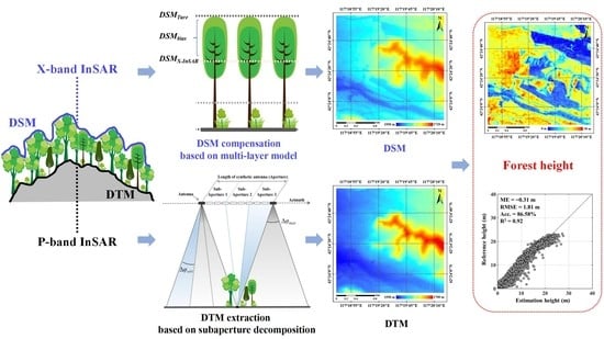
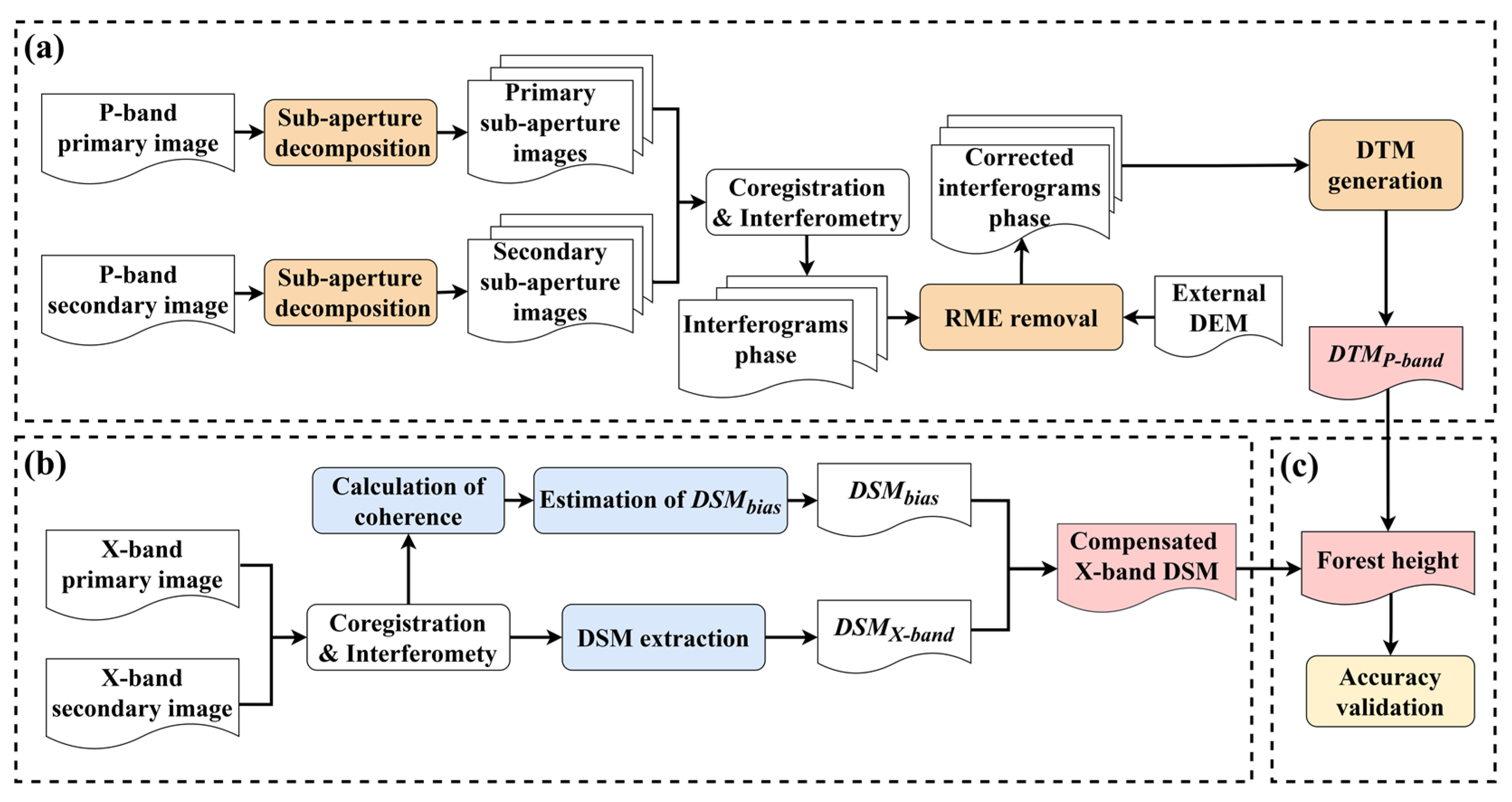
2. Methods

The proposed forest height estimation method mainly includes three steps, which are DTM extraction based on P-band InSAR, DSM extraction and compensation based on X-band InSAR and accuracy validation. The flowchart of the processing steps is given in Figure 2.

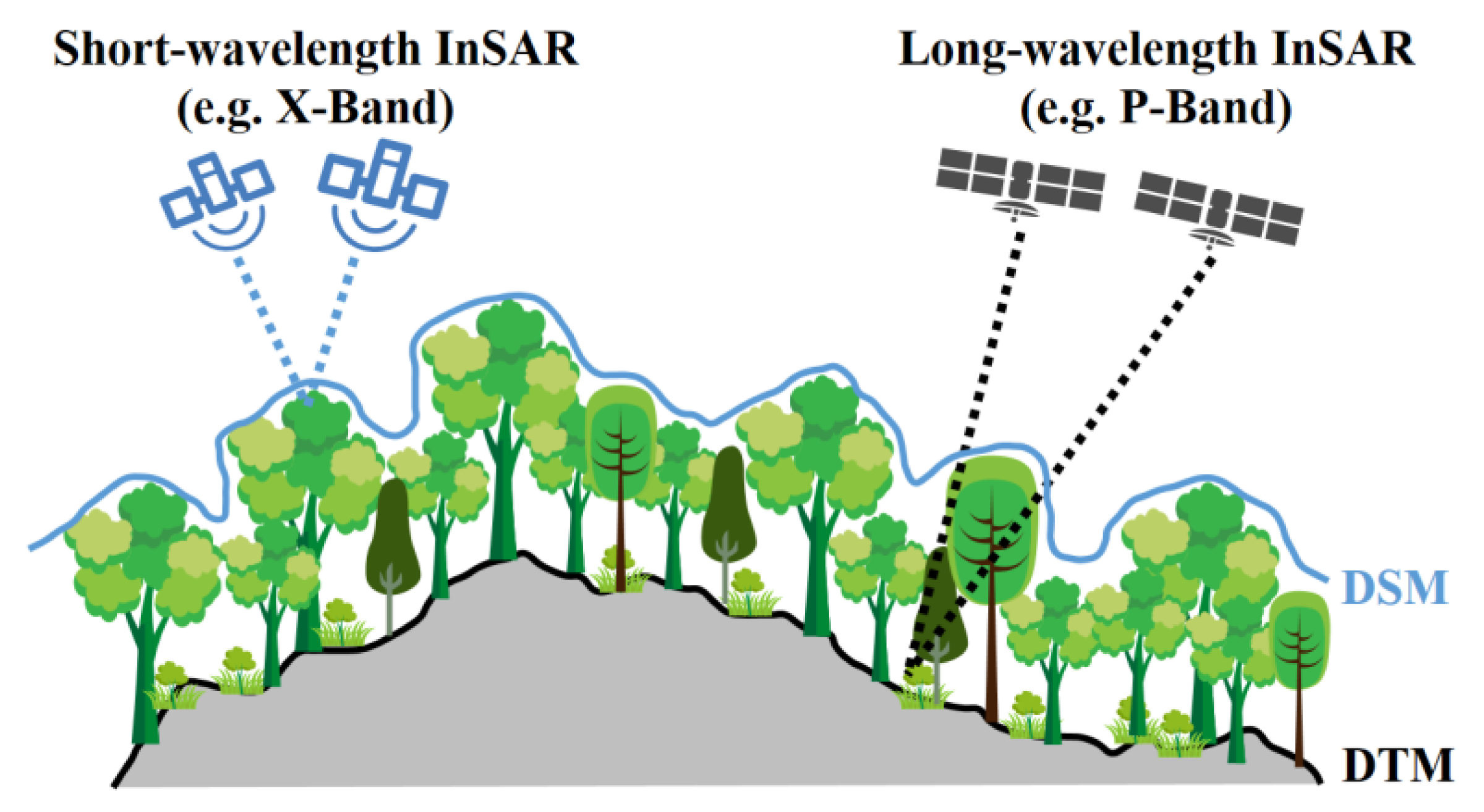
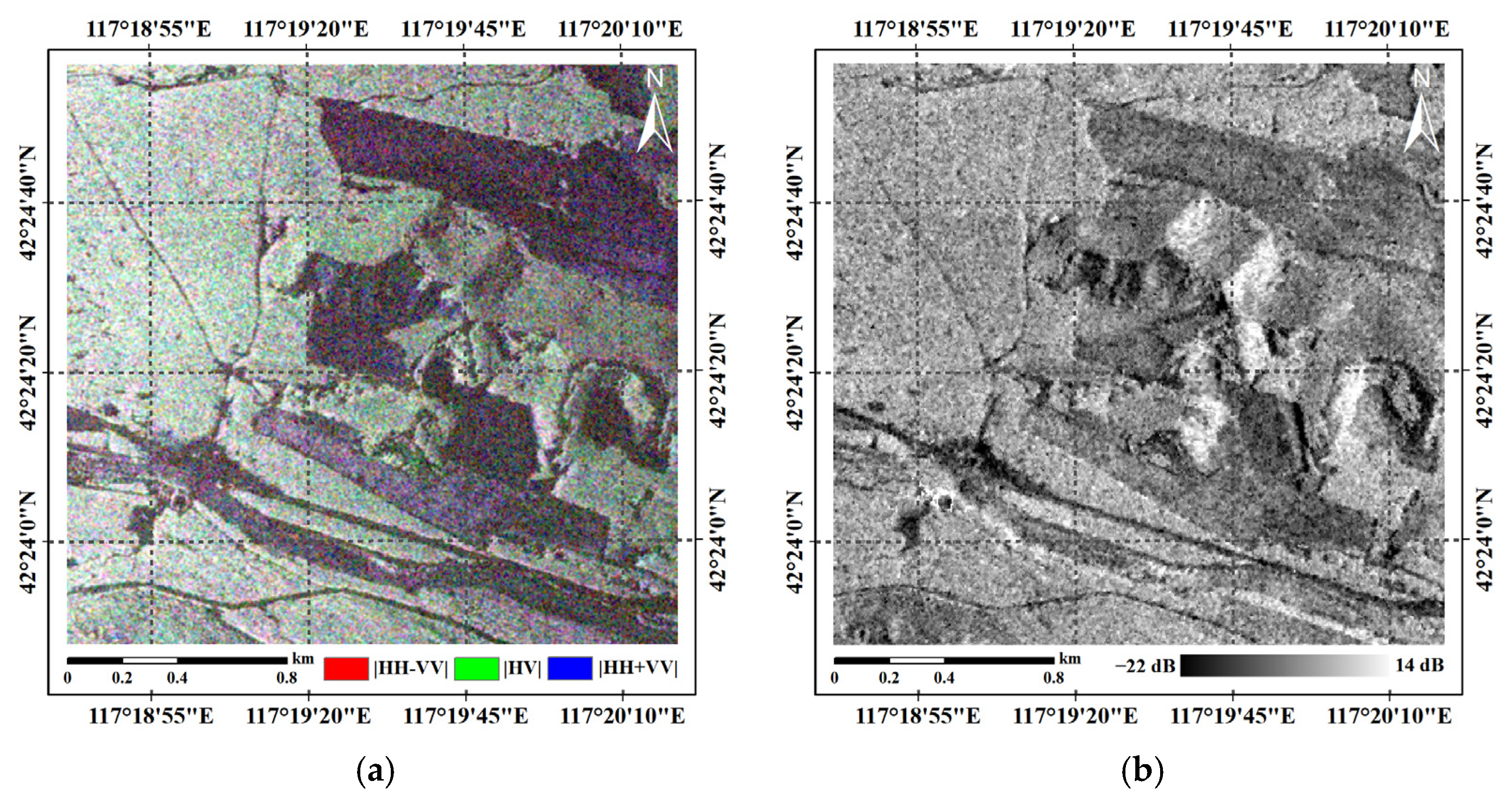
2.1. DTM Extraction Based on P-Band InSAR

2.1.1. Basic Idea of the TF Analysis Approach

For SAR, the method adopted to achieve high-resolution imaging in the azimuth direction is to synthesize an apparently long antenna by making use of the forward linear motion of a short antenna. Therefore, a target in a resolution cell is observed by a SAR sensor with a time-varying observation angle (φ) during the azimuthal integration. Furthermore, the amount of change (Δφ) in the observation angle has the following relationship with the resolution in the azimuth direction (δ_az) and the wavelength (λ) of SAR [17,18].

$$\Delta \phi =\frac{\lambda }{2{\delta }_{az}}$$

(1)

Based on Equation (1), it can be determined that high-resolution P-band SAR has a larger Δφ compared with short-wavelength SAR with the equivalent resolution. For example, if the λ is 66.70 cm and the δ_az is 1.00 m, then Δφ is easily calculated to be 0.33, which is close to 20°. For such a large observation angle range, the likelihood of the SAR sensor “seeing” the pure ground surface is low in a forest scene. In other words, the signal of the high-resolution P-band SAR contains more contributions from forest scatterers owing to the longer synthetic aperture. Therefore, the average phase center of the SAR signal is higher than the underlying surface. In order to extract the pure underlying ground phase, Garestier et al. proposed a TF analysis approach that obtains the subaperture images with the pure ground scattering contribution by changing the observation angle in the azimuth direction [17,32].

As shown in Figure 3, the subaperture has a smaller viewing angle (Δφ_sub2/3), so it is easier to “see” the pure ground surface than the full aperture (Δφ_max). Moreover, for different forest scenes, the difference in the viewing angle of different subapertures can also play a flexible role. However, the reduction of the aperture length also raises the problem of reduced resolution and more susceptibility to the residual motion error (RME) of the platform [18]. For the former, the influence can be reduced by flexibly setting the length of the subapertures. For the latter, Fu et al. proposed an improved TF analysis method, which can be used for the DTM extraction of P-band InSAR [18]. In general, DTM extraction based on the improved TF analysis method is divided into three steps: subaperture decomposition, RME removal and DTM generation.

2.1.2. Subaperture Decomposition

The subaperture decomposition is realized by a band-pass filter of the original single-look complex (SLC) image in the azimuth frequency domain and can be summed up as follows [33,34]:

$$S=FF{T}_{az}^{-1}[\omega (n)\times FF{T}_{az}(SLC)]$$

(2)

where S is the subaperture image, FFT_az and ${\mathit{FFT}}_{az}^{-1}$ represent the one-dimensional Fourier transform and the one-dimensional inverse Fourier transform in the azimuth direction, respectively. ω(n) represents the band-pass filter with a Hamming window and is designed as follows [35]:

$$\omega (n)=\begin{array}{ll}0.54-0.46\cos (2\pi \frac{n}{N-1})\hfill & 0\le n\le N\hfill \end{array}-1$$

(3)

where N is the window length of the Hamming window, and it is related to the number of extracted subapertures and the overlap ratio of the subapertures to the full aperture [33]. The specific implementation of subaperture decomposition refers to the program in the PolSARpro software (version: 6.0; Eric Pottier et al.; Rennes, France; https://earth.esa.int/eogateway/tools/polsarpro, accessed on 20 June 2022). In addition, unlike the nonoverlapping subapertures shown in Figure 3, the method of extracting subaperture images with certain overlap can enrich the observation angle variation and maintain an acceptable resolution.

2.1.3. RME Removal

Through subaperture decomposition, the ground can be “seen” more or less directly by the SAR sensor. However, it should be noted that different subapertures are affected differently by the local RME of the platform. Therefore, in the interferometric processing based on subaperture SAR images, the influence of the RME should be removed first. For the subaperture interferogram, the interferometric phase (φ_int) is composed of

$${\phi }_{int}={\phi }_{flat}+{\phi }_{topo}+{\phi }_{forest}+{\phi }_{noise}+{\phi }_{RME}$$

(4)

where φ_flat and φ_topo are the flat-earth phase and topographic phase, respectively. φ_forest is the phase caused by the forest components, and φ_noise is the random error phase. φ_RME is the phase caused by the motion error.

Firstly, φ_flat and φ_topo can be removed based on the globally shared digital elevation model (DEM) data, such as the SRTM DEM, ASTER DEM, etc. [36]. In this step, there is also a topographical residual phase (Δφ_topo) in φ_int owing to the error of the input DEM. Secondly, it is recommended to use wavelet decomposition to remove some components of Δφ_topo, φ_forest and φ_noise, which are high frequency components in the interferogram compared to φ_RME [18]. The process also reduces the influence of vertical precision for the SRTM DEM or the ASTER DEM used in the previous step. After the above two steps, the phase information in the interferogram is mainly φ_RME. Then, for each row datum of azimuth direction, the one-dimensional polynomial fitting in the range direction is used to reduce the influence of the phase error caused by the baseline error in the range direction [18]:

$${\phi }_{RME}x,y={\displaystyle {\sum }_{i=0}^n{a}_i\cdot y^i}+b\cdot h$$

(5)

where x, y are the azimuth and slant range coordinates, respectively. n is the order of the polynomial. a_i and b are the unknown coefficients, and h is the elevation information obtained by the input DEM. Finally, the relatively pure φ_RME is obtained and can be easily removed from the subaperture interferograms by complex conjugate multiplication. Specifically, first, φ_RME can be converted into a complex form based on Euler’s formula [37]. Then, φ_RME can be removed by complex conjugate multiplication between subaperture interferograms and φ_RME in complex form [37].

2.1.4. DTM Generation

After the above processing steps, each pixel of the SAR data contains several interferometric phases corresponding to different subapertures. We then need to determine which subaperture corresponds to the interferometric phase that is the optimal ground phase. Here, we selected the subaperture whose interferometric phase had the largest difference from the interferometric phase of the volume-dominated polarization channel of the full aperture data. Subsequently, the extraction of the DTM is the same as that of the conventional InSAR measurement of the DEM, that is, it includes steps such as filtering, phase unwrapping, and phase-height conversion [18].

2.2. DSM Extraction and Compensation Based on X-Band InSAR

2.2.1. Bias of DSM Extraction Based on X-Band InSAR

Based on conventional interferometric processing (i.e., registration, filtering, unwrapping, phase-height conversion, etc.), the initial version of the DSM can be extracted based on X-band InSAR data, denoted as DSM_X-InSAR. As shown in Figure 4a, because of the radar signal penetration, there is a bias (DSM_bias) between the DSM_X-InSAR and the true values of DSM (DSM_True), that is:

$$DS{M}_{True}=DS{M}_{\text{X-InSAR}}+DS{M}_{bias}$$

(6)

Therefore, the accurate estimation of DSM_bias is the critical step for obtaining an accurate DSM and subsequently extracting the forest height by the difference based on the DTM extracted by P-band InSAR.

In order to estimate the DSM_bias, it is first necessary to model the forest stand and the scattering behavior of X-band InSAR in the forest area. Then, the inversion of DSM_bias is completed by establishing a mathematical relationship between DSM_bias and the interferometric coherence (γ). In the following, two estimation methods of DSM_bias will be introduced: one is the published method based on the IDUV model [21], and the other is the method based on the MLM model proposed in this paper.

2.2.2. Estimation Method of Bias Based on IDUV

Estimation Model

As shown in Figure 4b, the IDUV model is similar to the RVoG model, which assumes that the forest is a layer of uniform density without gaps. The scattering mechanism of X-band is a dielectric penetration process characterized by the mean extinction coefficient (κ). The thickness of the vegetation layer is also the maximum penetration depth and is denoted as D_max. Clearly, the vegetation layer shown in Figure 4b is still a finite depth uniform volume. When D_max tends toward positive infinity (D_max → +∞), the IDUV model can be derived and written as [21,25]:

$$\gamma =\frac{1}{2}+\frac{1}{2}\frac{1-j2\pi d_2/HoA}{1+j2\pi d_2/HoA},d_2=\frac{\cos \theta }{2\kappa }$$

(7)

where d₂ is the two-way penetration depth, θ is the incidence angle, and HoA is the height of ambiguity, which is defined as

$$HoA=2\pi /k_z$$

(8)

where k_z is the vertical wavenumber, which for a single-pass InSAR system is

$$k_z=2\pi B_n/\lambda R\sin \theta$$

(9)

where B_n is the perpendicular baseline, λ is the wavelength, R is the slant range.

Based on the geometric relationship of the IDUV model in the complex plane, the normalized interferometric phase (∠γ) corresponding to DSM_bias can be obtained through certain analysis and derivation [25]:

$$\angle \gamma =\mathrm{sgn}\left(HoA\right)\arctan \left(\sqrt{{\left|\gamma \right|}^{-2}-1}\right)$$

(10)

where sgn() is the sign function that returns the symbol of the input number.

Therefore, DSM_bias can be obtained as follows:

$$DS{M}_{bias}=\frac{\angle \gamma }{k_z}=\frac{\left|HoA\right|}{2\pi }\arctan \left(\sqrt{{\left|\gamma \right|}^{-2}-1}\right)$$

(11)

Based on Equation (11), it can be determined that the upper limit of DSM_bias estimated based on the IDUV model is equal to one-fourth of the HoA. Obviously, this is not a reasonable limit for diverse forests.

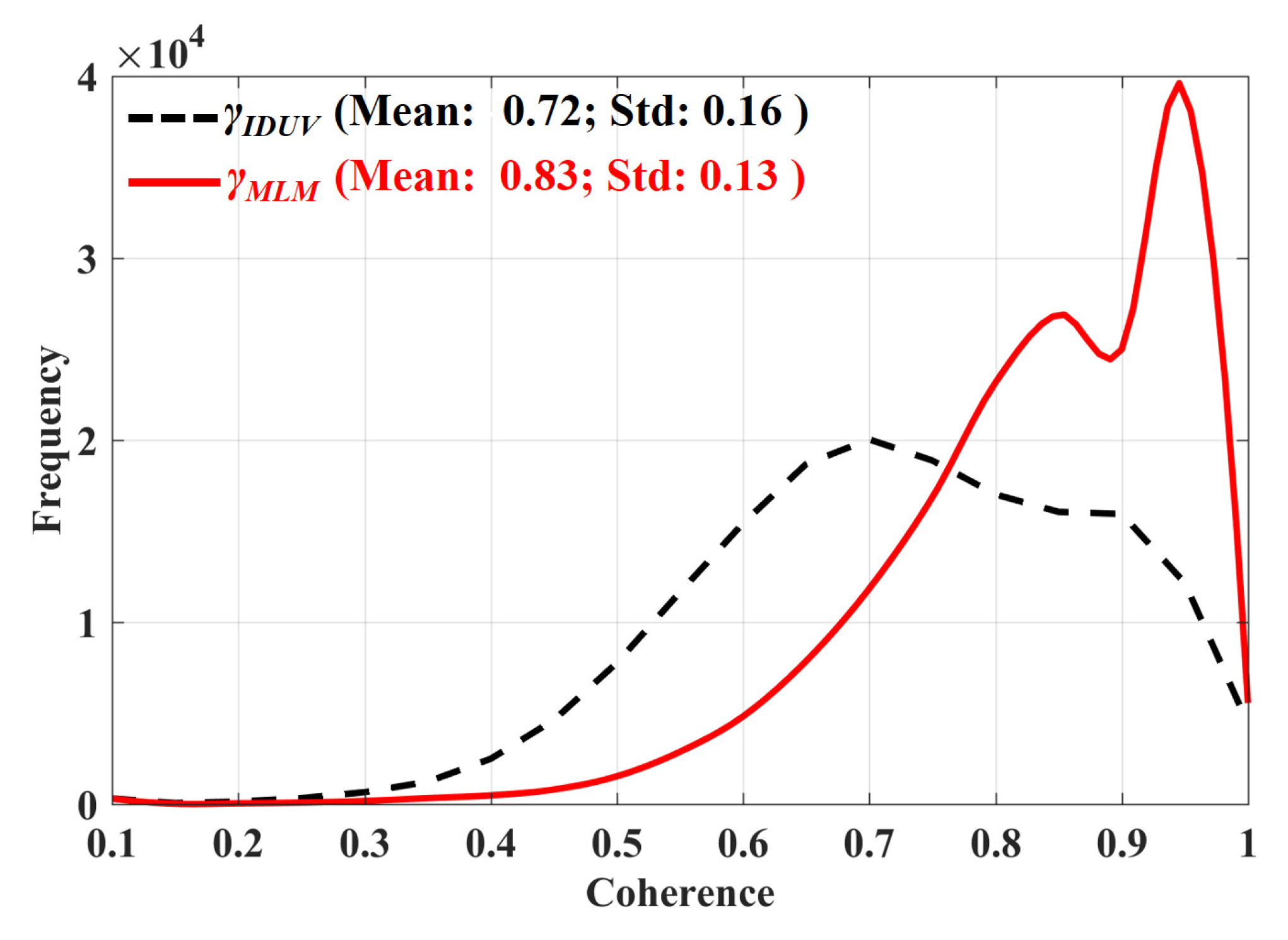
Calculation of Coherence for IDUV

Based on Equation (11), DSM_bias can be easily calculated using the coherence obtained from X-InSAR data. For the IDUV model, the observed coherence (γ_IDUV) is calculated using the following formula:

$${\gamma }_{IDUV}=\left|{\displaystyle \sum _{i=1}^N\sqrt{s_{1,i}{s}_{2,i}}\cdot e^{j{\phi }_{int,i}}\cdot e^{-j{\phi }_{flat,i}}\cdot e^{-j{\phi }_{topo,i}}}\right|/\sqrt{{\displaystyle \sum _{i=1}^N{s}_{1,i}\cdot {\displaystyle \sum _{i=1}^N{s}_{2,i}}}}$$

(12)

where N is the number of pixels of the estimated window, s₁ and s₂ represent the backscattering coefficients of the primary and secondary images, respectively. As shown in Equation (12), combined flat-earth and topographic phase removal should be performed prior to coherence estimation.

In addition, it should be noted that the input coherence for the IDUV model is the decorrelation from volume scattering, therefore, other decoherence factors need to be removed, such as decorrelation from the signal-to-noise ratio (SNR) [21].

2.2.3. Estimation Method of Bias Based on the MLM

General Estimation Method

The MLM is a theoretical model of coherence with generalized properties that only considers the gap penetration of radar signals. In the model, forest is assumed as multi-layers of negligible thickness without dielectric penetration (Figure 4c). Originally, the MLM was proposed for the inversion of forest height [28]. In this case, it was assumed that the radar signal of X-band InSAR penetrates the forest and reaches the ground surface, that is, it was assumed that D_max in Figure 4c is equal to the forest height. In this paper, we will further expand the application scope of the MLM, that is, D_max can be less than or equal to the forest height, so that it can be used for DSM_bias estimation of diverse forests.

The original MLM model is derived from the maximum likelihood estimator of coherence based on the following three assumptions [28]:

Assumption 1.

The backscattering coefficients of the primary and secondary images are equal.

Assumption 2.

A combined flat-earth and topographic phase removal prior to the coherence estimation is performed.

Assumption 3.

The backscattering coefficients of the pixels at same heights are equal.

First, we need to replace the forest height (H) in the original MLM model with the maximum penetration depth (D_max), namely:

$$\gamma =\frac{\left|{\displaystyle {\int }_0^{D_{max}}f(x)\sigma (x)e^{j{k}_{z}x}dx}\right|}{{\displaystyle {\int }_0^{D_{max}}f(x)\sigma (x)dx}}$$

(13)

where f(x) is a continuous probability density function (PDF) with the interval (0, D_max), which reflects the location distribution of scatter in the vertical direction. σ(x) represents the backscattering coefficient of scatterers at different penetration depths. Then, to further simplify Equation (13), we assumed that σ(x) is a constant. That is, the fourth assumption:

Assumption 4.

The backscattering coefficients of the pixels at different heights are equal.

Then, Equation (13) can be simplified as

$$\gamma =\left|{\displaystyle {\int }_0^{D_{max}}f(x)e^{j{k}_{z}x}dx}\right|$$

(14)

For Equation (14), when f(x) is a known definite PDF, D_max can be obtained by further model simplification or iterative search [28]. After the inversion of D_max, it is further necessary to determine the average penetration depth (D_mean, in Figure 4c) of the X-band SAR signal over the interval (0, D_max). The D_mean is actually equal to the mathematical expectation of the depths of the scatterers at different levels, that is,

$$D_{mean}={\displaystyle {\int }_0^{D_{max}}xf(x)dx}$$

(15)

Based on Equations (14) and Equation (15), the estimation of D_mean can be achieved, and DSM_bias is numerically equal to D_mean. Obviously, choosing a suitable f(x) is critical for estimating DSM_bias based on the MLM model.

Special Case Based on Uniform Distribution

If we assume that f(x) is the PDF of a uniform distribution with the interval (0, D_max), it is defined as

$$f\left(x\right)=\frac{1}{D_{max}},x\in \left(0,D_{max}\right)$$

(16)

Then, inserting Equation (16) into Equation (14) yields

$$\gamma =\frac{\sin \left(k_z{D}_{max}/2\right)}{k_z{D}_{max}/2}{e}^{j{k}_z{D}_{max}/2}$$

(17)

Furthermore, the inversion model of D_max can be obtained [5,28]:

$$D_{max}=\frac{2\pi }{\left|k_z\right|}\left(1-\frac{2}{\pi }{\sin }^{-1}\left[{\left|\gamma \right|}^{0.8}\right]\right)$$

(18)

Furthermore, inserting Equation (16) into Equation (15) yields

$$D_{mean}=\frac{1}{D_{max}}\cdot \frac{1}{2}{x^2|}_0^{D_{max}}=\frac{1}{2}{D}_{max}$$

(19)

Therefore, we get the estimated formula for DSM_bias:

$$DS{M}_{bias}=D_{mean}=\frac{\pi }{\left|k_z\right|}\left(1-\frac{2}{\pi }{\sin }^{-1}\left[{\left|\gamma \right|}^{0.8}\right]\right)$$

(20)

Calculation of Coherence for the MLM

As opposed to traditional models such as IDUV and RVoG, the coherence in the MLM model does not mean the pure volume scattering decorrelation. In MLM-based parameter inversion, the priority is not to remove other decorrelation factors, but to emphasize that the calculation of coherence need to meet the assumptions of the theoretical model of coherence as much as possible. Based on this consideration, Zhao et al. proposed a coherence calculation method suitable for the MLM model [28], that is,

$${\gamma }_{MLM}=\left|\frac{1}{N}{\displaystyle \sum _{i=1}^N{e}^{j{\phi }_{int,i}}\cdot e^{-j{\phi }_{flat,i}}\cdot e^{-j{\phi }_{topo,i}}}\right|$$

(21)

γ_MLM satisfies the four Assumptions 1–4 in the derivation of the MLM simplified model. It was proven in [28] that in the forest height inversion based on the MLM model the γ_MLM can achieve better accuracy than the traditional coherence calculation method (γ_IDUV). Predictably, γ_MLM should have the same effect on the estimation of DSM_bias based on the MLM.

2.3. Accuracy Validation

To comprehensively evaluate the accuracy of the proposed approach, four evaluation indicators were selected in this paper. As

Table 1. The evaluation index used in this paper *.

Evaluation Index	Symbol	Formula	Ideal Value
Mean Error	ME	$\frac{1}{n}{\displaystyle \sum _{i=1}^n\left(x_i-y_i\right)}$	0
Root Mean Square Error	RMSE	$\sqrt{\frac{1}{n}{\displaystyle \sum _{i=1}^n{\left(x_i-y_i\right)}^2}}$	0
Accuracy	Acc.	$\left(1-\frac{\mathrm{RMSE}}{E\left(y_i\right)}\right)\cdot 100\%$	100%
Coefficient of Determination	R2	$1-{\displaystyle \sum _{i=1}^n{\left(x_i-y_i\right)}^2}/{\displaystyle \sum _{i=1}^n{\left(E(y_i)-y_i\right)}^2}$	1

* x_i and y_i are the estimation value and reference value, respectively. n is the number of samples. E() denotes mathematical expectation.

shows, these indicators are the mean error (ME), root mean square error (RMSE), accuracy (Acc.) and coefficient of determination (R²).

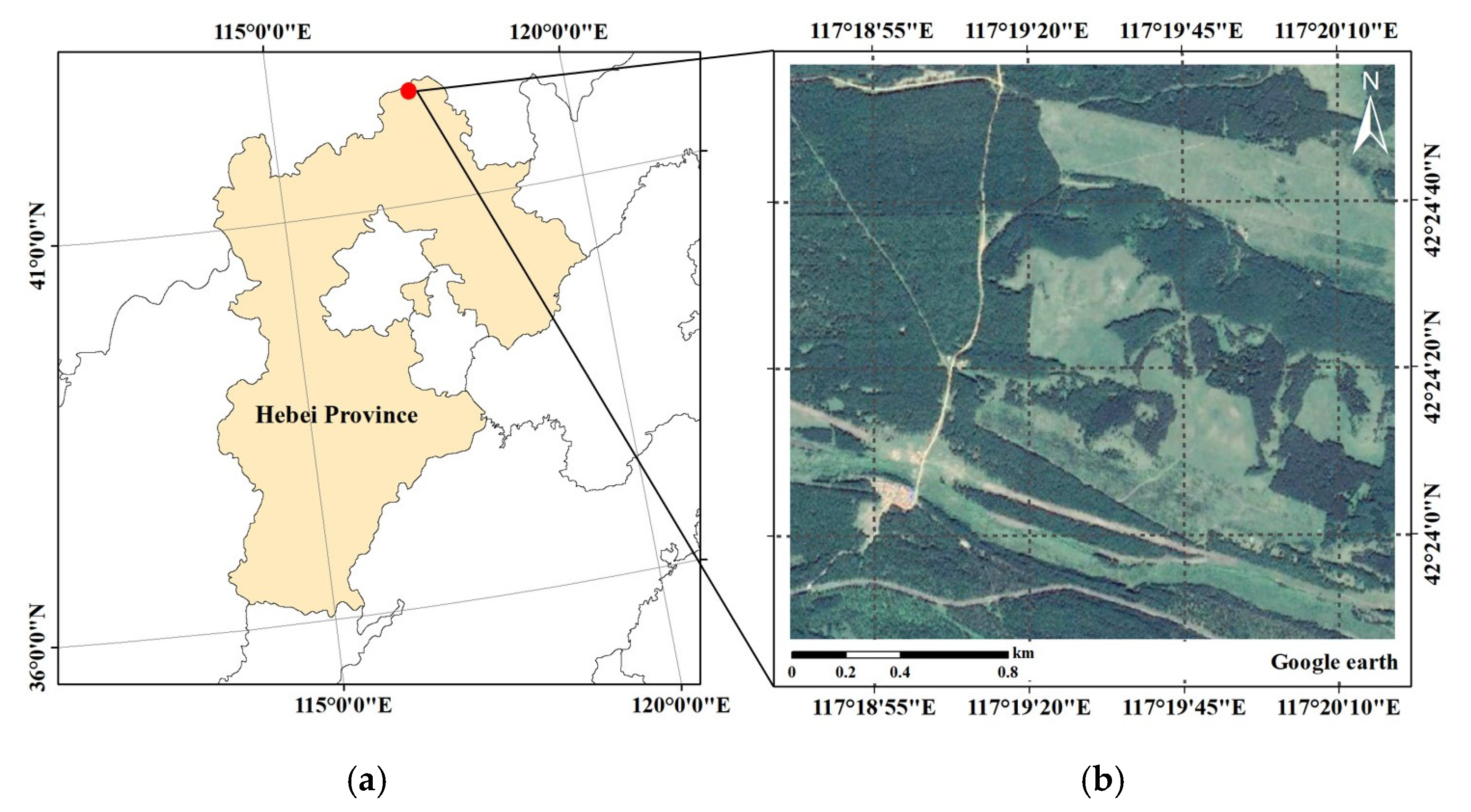
3. Study Area and Data

3.1. Study Area

The study was conducted at Saihanba Forest Farm located in the north of Hebei Province, China. As shown in Figure 5, the geographical location of the study area is 117°18′45″E to 117°20′20″E and 42°23′48″N to 42°24′55″N. The width (east–west) of the area is about 2.2 km and length (north–south) is about 2.1 km. It lies in the junction of the northern Hebei Province mountainous areas and the Inner Mongolian plateau, with altitudes ranging from 1550 to 1700 m. Both coniferous forest and broad-leaved forest are distributed in the area and predominant tree species of the forests are Pinus sylvestris var. mongolica Litv., Betula platyphylla Suk., and Larix gmelinii (Rupr.) Kuzen.

3.2. InSAR Data

In the study area, the InSAR data of P-band and X-band were acquired. The P-band InSAR data were acquired on 29 October 2019, based on the airborne SAR system using the repeat-pass mode. The P-band airborne SAR system was independently developed by the Aerospace Information Research Institute, Chinese Academy of Science. The speed of the airborne platform was about 80 m/s with the flying height about 4000 m. The acquisition time difference between the primary image and the secondary image of P-band InSAR was about 30 min. In addition, the X-band single-pass InSAR data were acquired on 29 December 2018, based on the TanDEM-X system, which is a well-known European spaceborne InSAR system. The details of the acquired P-band and X-band InSAR data are presented in

Table 2. Parameters of acquired P-band and X-band InSAR data *.

Parameters	P-Band	X-Band
Frequency	0.45 GHz	9.65 GHz
Polarization	HH/HV/VH/VV	HH
Center Incidence Angle	63°	43°
Spatial baseline	60.25 m	332.77 m
HoA (mean)	81 m	44 m
SLC Resolution (a × r)	1.45 m × 1.50 m	2.21 m × 1.36 m

* HoA, height of ambiguity; SLC, single-look complex.

.

The Pauli RGB of the P-band primary image over the study area is shown in Figure 6a. Figure 6b presents the intensity information of the X-band primary image.

3.3. LiDAR Data

Airborne LiDAR data were acquired from the study area with the full waveform laser scanner (LMS-Q680i, Riegl, Horn, Austria) of the CAF-LiCHY (Chinese Academy of Forestry-LiDAR, CCD and Hyperspectral) system around September 2018 [38,39]. Subsequently, LiDAR products, including the DTM, DSM and canopy height model (CHM) were obtained from the LiDAR point cloud data. The LiDAR DTM, DSM, and CHM are shown in Figure 6a–c. The spatial resolution of the above LiDAR product was 2 m, which was similar to the SLC resolution of the P-band and X-band InSAR data (Table 2). It should be noted that both P-band and X-band InSAR data involve some down-resolution processing steps such as multi-look, filtering, etc. Therefore, for the final accuracy assessment of forest height, the 100th percentile heights (H₁₀₀) data with a suitable filtering window size should be extracted based on LiDAR CHM data. The H₁₀₀ data of the study area were obtained using the maximum filtering method with the 18 m × 18 m filter window, as shown in Figure 7d. That is, it corresponded to the 3 × 3 multi-look window and the 3 × 3 filtering window of the SAR data process. It should be noted that the pixel size of H₁₀₀ remained the same as the above LiDAR product, that is, 2 m.

4. Data Processing

4.1. DTM Extraction Process

The DTM extraction process began with SLC images of P-band InSAR data, and as mentioned before, mainly included three steps: subaperture decomposition, RME removal and DTM generation.

For P-band polarimetric InSAR data used in this paper, we first needed to select a polarization channel with the strongest penetration ability into the forest, and previous studies have shown that HH polarization is the better choice [17]. Then, based on P-band InSAR data of HH polarization, five subaperture images of equivalent resolution with 50% overlap (each subaperture was a third of the full aperture) were generated for both primary and secondary images. Subsequently, the co-registrations between the primary and secondary images of the same subaperture were completed with the accuracy of 0.02~0.03 pixels in range and 0.05~0.06 pixels in azimuth. Then, the interferograms of the subaperture InSAR pairs were completed with a 3 × 3 multi-look window size.

In the RME removal, φ_flat and φ_topo were generated and removed from the interference phase of each subaperture based on the image parameters (interferometric baseline, slant range and incidence angle) of the InSAR system and SRTM DEM data [36]. Then, the level 1 wavelet decomposition with Haar wavelet basis was performed for removing Δφ_topo, φ_forest and φ_noise. Subsequently, φ_RME was fitted according to a three-order (n = 3) polynomial based on Equation (5). Finally, the effect of RME was removed by multiplying φ_RME by the complex conjugate of the original subaperture interferograms.

For the DTM generation, the subaperture whose interferometric phase had the largest difference with the interferometric phase of the HV polarization in the full aperture data was selected as the optimal ground phase for every pixel. Then, to reduce the phase noise, the optimal ground phase was filtered with a modified Goldstein filter with a 3 × 3 window size [40]. Next, the filtered phase was unwrapped using the minimum cost flow (MCF) method [41]. Finally, the P-band DTM (DTM_P-band) was obtained by linear function of phase-height conversion [36].

In terms of the noise level of the P-band SAR data used, the equivalent number of looks (ENL) for the SLC level was 0.90, and the ENL after multi-looking and filtering was 13.51.

4.2. DSM Extraction and Compensation Process

The processing of DSM extraction and compensation was mainly divided into two steps, which were the extraction of the initial DSM version (DSM_X-InSAR) and the estimation of DSM_bias.

For the extraction of DSM_X-InSAR, the first step was co-registration. Since the InSAR data of the TanDEM-X system undergo co-registration before they are provided to users, the step can be skipped and the extraction processing begun with interferogram generation using the SLC images of TanDEM-X InSAR data. The interferogram was completed with a 3 × 3 multi-look window size. Then, the flat-earth phase was calculated and removed based on the image parameters of the InSAR system [36]. Subsequently, the flattened InSAR phase was filtered with the Goldstein filter with a 3 × 3 window size reducing the phase noise [40]. Next, the MCF algorithm was used for phase unwrapping [41]. Finally, DSM_X-InSAR was extracted by linear function of phase-height conversion based on the unwrapped phase [36].

For the estimation of DSM_bias, the first step was the calculation of coherence. Before the calculation, the combined flat-earth and topographic phase was calculated and removed according to the image parameters of the InSAR system and the DTM_P-band previously extracted [36]. Then, γ_IDUV and γ_MLM were estimated according to Equation (12) and Equation (21), respectively. The estimated window size of both estimations was 3 × 3. Since the main decoherence factors of the TanDEM-X InSAR data were the SNR ratio and volume scattering [12,42], the influence of SNR was removed by dividing γ_IDUV by the SNR decorrelation, which was computed based on the backscattering intensity and noise equivalent sigma zero (NESZ) provided as the image parameters for every TanDEM-X acquisition [42].

For the IDUV model, DSM_bias was estimated according to Equation (11) based on γ_IDUV, and the compensated DSM based on IDUV (DSM_X-IIDUV) was obtained by adding DSM_bias to DSM_X-InSAR. Similarly, for the MLM, the compensated DSM based on the MLM (DSM_X-MLM) was formed by adding the DSM_bias of the MLM to DSM_X-InSAR. The DSM_bias of the MLM in the special uniform distribution case was estimated according to Equation (20), based on γ_MLM.

In terms of the noise level of the X-band SAR data used, the ENL for the SLC level was 0.84, and the ENL after multi-looking and filtering was 19.64.

4.3. Forest Height Estimation and Accuracy Validation

The final forest height estimation results were completed by subtracting DTM_P-band from different X-InSAR DSMs. The pixel size of P-band and X-band InSAR products was 6 m × 6 m (coordinate: UTM zone 50N), which was decided according to the pixel size of InSAR SLC data (about 2 m) and the parameters of the multi-looking process (3 × 3 window size).

The accuracy verification was based on the InSAR product with a 6 m × 6 m pixel size and the LiDAR product with a 2 m × 2 m pixel size. For each pixel of the InSAR product to be evaluated, we first found the LiDAR pixel located at the center of the pixel of InSAR product. Then, taking this LiDAR pixel as the center, all LiDAR pixels within the actual range corresponding to the pixel of InSAR product were used for verification. Since there are 3 × 3 window size multi-look and 3 × 3 window size filtering involved in the InSAR procedures, each pixel of InSAR products contained the information corresponding to an area of about 18 m × 18 m. Therefore, although the pixel size of the InSAR product was 6 m × 6 m, the LiDAR-based verification value was calculated based on all LiDAR pixels within 18 m × 18 m. For the validation of the DTM, the validation value was the mean of all LiDAR DTM pixels within the 18 m × 18 m. For the validation of forest height, the validation value was the maximum value of all LiDAR CHM pixels within the 18 m × 18 m, as displayed by Figure 7d in the previous section. For the validation of the DSM, the verification value was the sum of the above two values.

For the validation of forest height estimation results, a total of 2631 samples were extracted systemically with 42 m intervals. In fact, at 42 m intervals, a total of 2754 samples could be extracted, and 123 samples from non-vegetated areas (H₁₀₀ < 0.5 m) were removed, and the remaining 2631 samples were evenly distributed in the study area.

The above steps were completed using GAMMA software (version: 2012; GAMMA Remote Sensing corporation, Gumligen, Switzerland; https://www.gamma-rs.com/, accessed on 20 June 2022), PolSARpro software and our own program. The software and program were run on a computer with AMD Ryzen 7 5800H CPU and NVIDIA GeForce RTX 3060 GPU.

5. Results

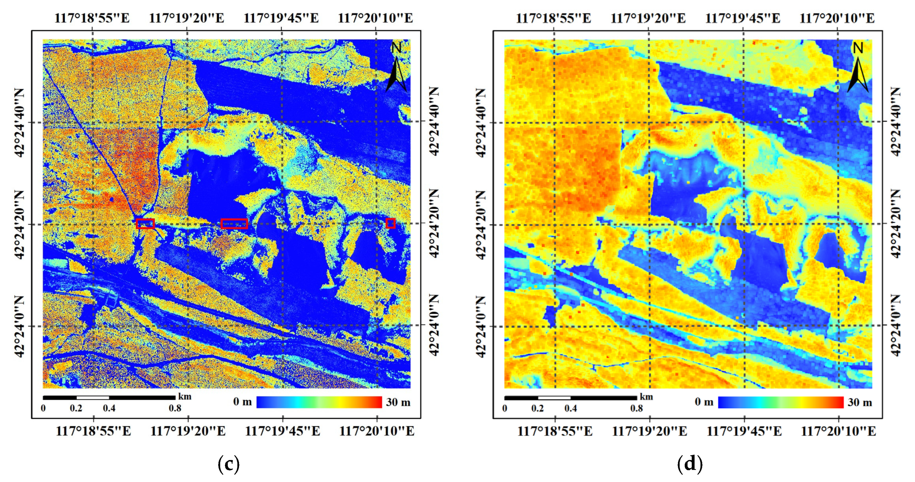
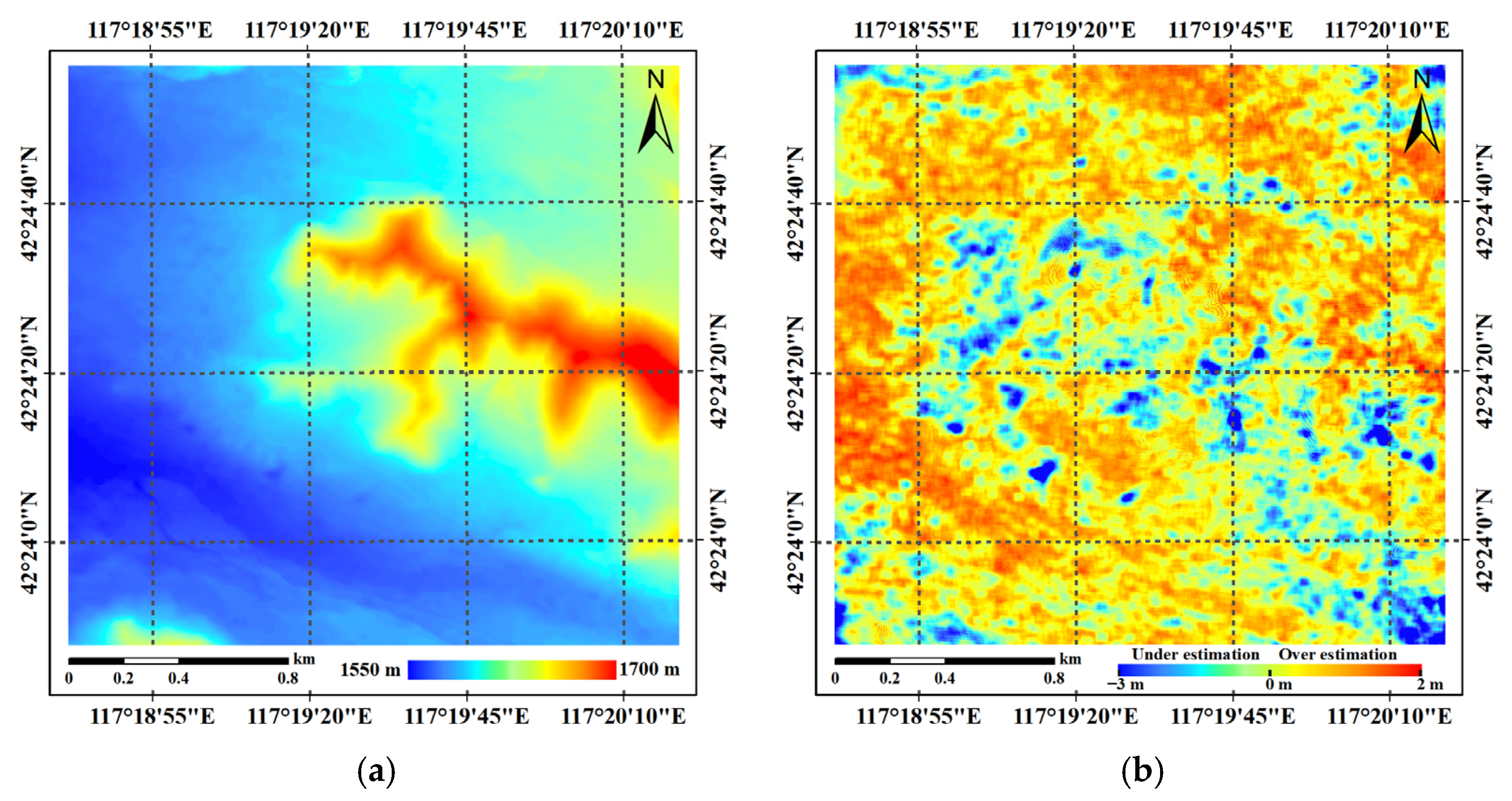
5.1. DTM Extraction from P-Band InSAR Data

The final DTM_P-band is displayed in Figure 8a. It can be seen that DTM_P-band and DTM_LiDAR (Figure 7a) presented similar patterns, with elevation ranging from 1550 to 1700 m. Figure 8b shows the difference between DTM_P-band and DTM_LiDAR. Figure 9 shows the histogram of the difference. It can be observed that the differences were mainly distributed between −3 and 2 m. There was no obvious relation between the areas of large differences with their land-cover type, vegetation height, altitude or other factors. In our opinion, the main reason behind the differences was the effect of random errors in the overall process, such as the residual phase error of RME. The ME of DTM_P-band was 0.14 m, and the RMSE was 0.94 m. According to H₁₀₀ (Figure 7d), the forest height in the study area was about 10 to 30 m. This suggested that the accuracy of the extracted DTM was sufficient for the forest height estimation. In addition, a study [18] achieved DTM extraction accuracy with an RMSE of 2.01 m based on the same TF method.

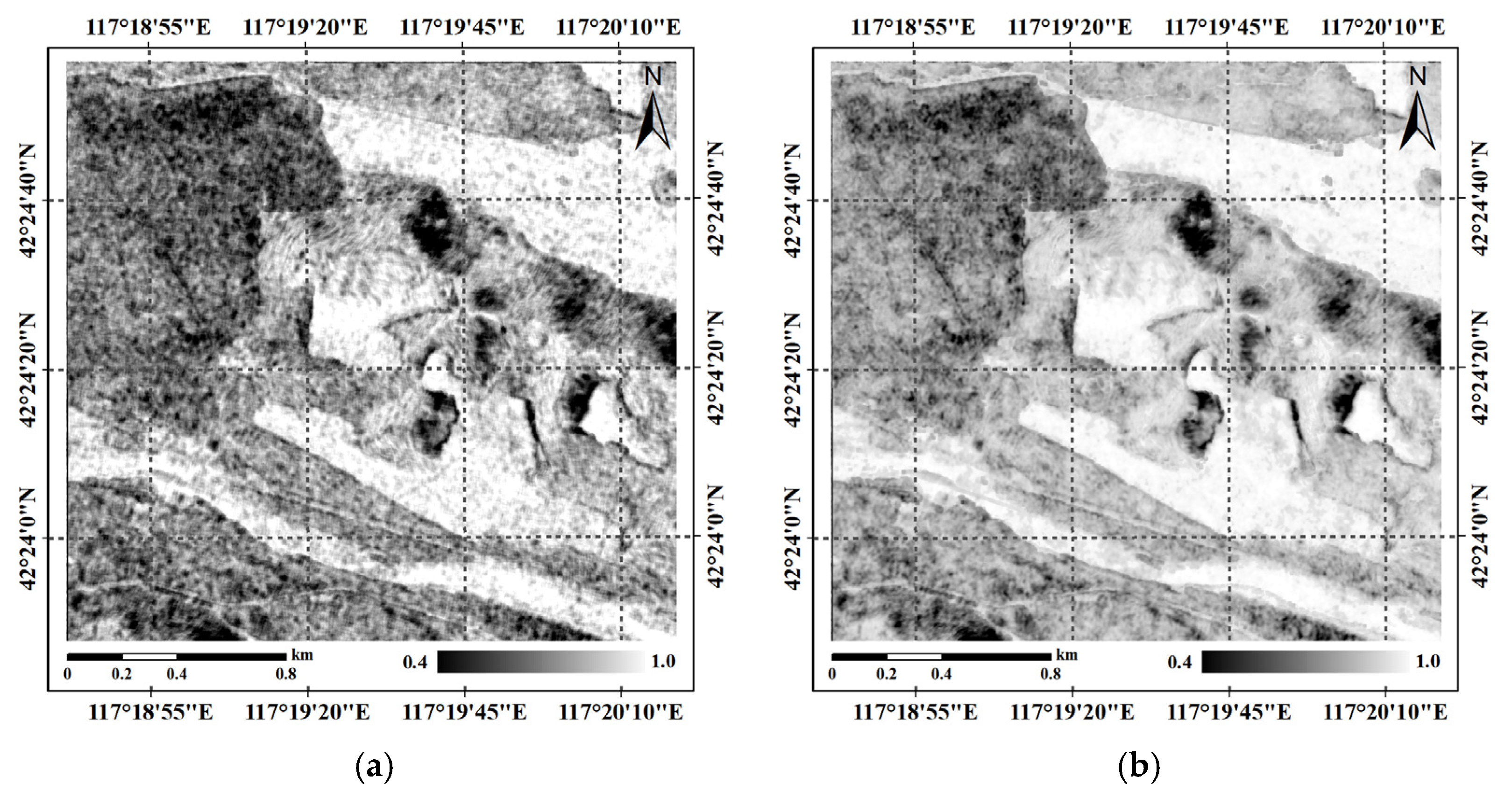
5.2. DSM Extraction and Compensation from X-Band InSAR Data

5.2.1. Raw Result of DSM Extraction

The initial DSM version (DSM_X-InSAR) is displayed in Figure 10a. It can be seen that DSM_X-InSAR and DSM_LiDAR (Figure 7b) presented similar patterns. The differences between DSM_X-InSAR and DSM_LiDAR are shown in Figure 10b. For most forest-covered area, the differences were lower than −5 m and down to −15 m, indicating DSM_X-InSAR had a clear underestimation compared to DSM_LiDAR. The main reason behind the large deviation was the non-negligible penetration ability of X-band InSAR into the forests. In areas where the forest height is high enough (e.g., >20 m), large enough gaps in the forest stand allowing the SAR signal to penetrate the underlying surface are enough to generate a large InSAR DSM error (e.g., ~15 m). The study [12] also found a substantial penetration of up to 12 m in a boreal forest with TanDEM-X data. The large deviation between DSM_LiDAR and DSM_X-InSAR suggested that, for accurate forest height estimation, the bias of DSM_X-InSAR should be compensated.

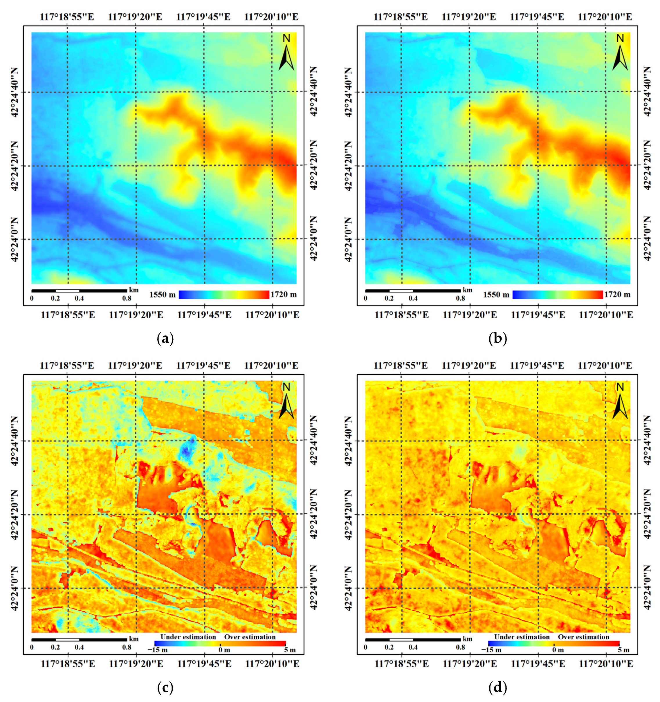
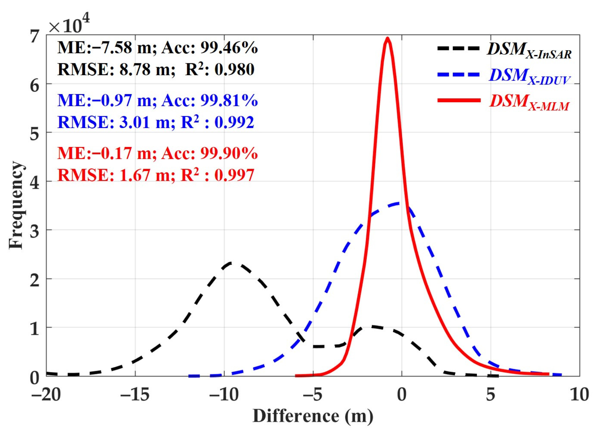
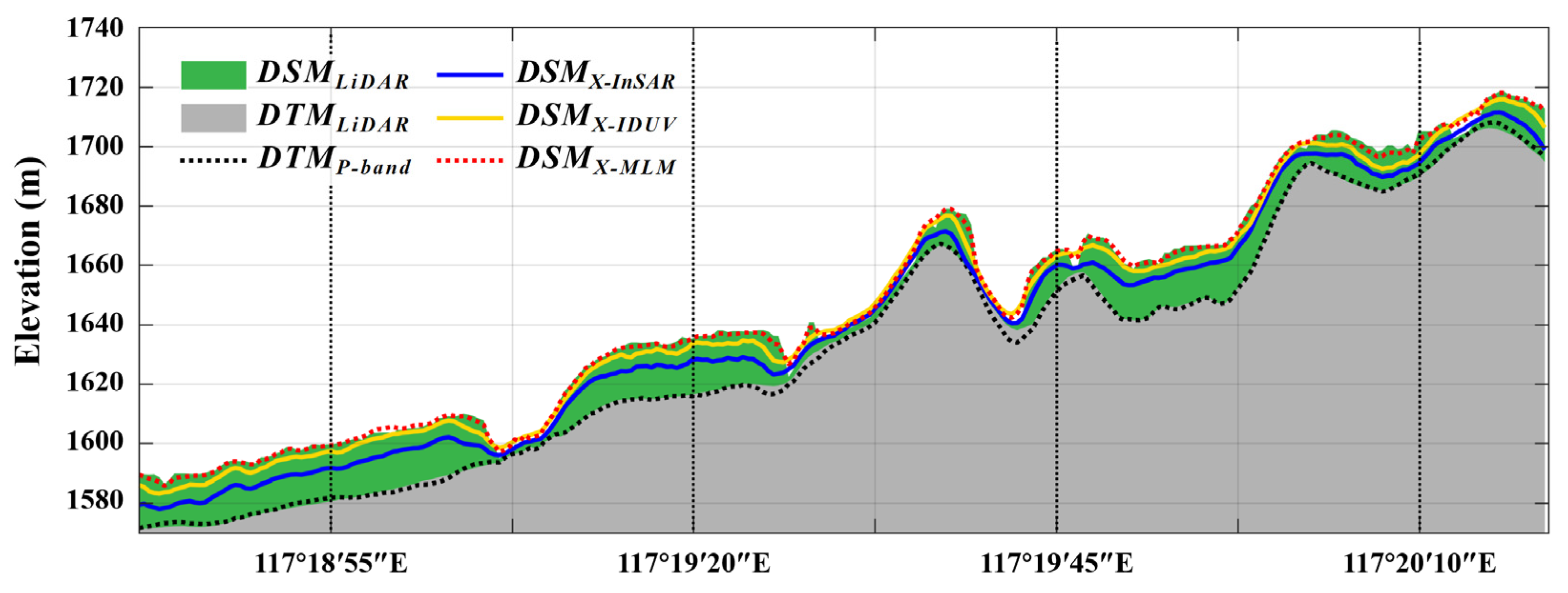
5.2.2. DSM Compensation Result

The calculation results of coherence (γ_IDUV and γ_MLM) are displayed in Figure 11a and Figure 11b, respectively. Overall, it is clear that the coherence level of γ_MLM was greater than that of γ_IDUV. Figure 12 presents the histogram of both coherence images. Compared with γ_IDUV, γ_MLM had a higher mean and lower standard deviation (Std).

DSM_X-IDUV and DSM_X-MLM are displayed in Figure 13a and Figure 13b, respectively. Both DSM_X-IDUV and DSM_X-MLM have similar distribution trends to DSM_LiDAR (Figure 7b). Figure 13c shows the difference between DSM_X-IDUV and DSM_LiDAR. Compared to the differences between DSM_X-InSAR and DSM_LiDAR (Figure 10b), the DSM underestimation of forest area was corrected effectively. However, for the area where the differences between DSM_LiDAR and DSM_X-InSAR were lower than −10 m (appearing in blue in Figure 10b), DSM_X-IDUV still had an underestimation of about 5 to 10 m, which will result in a large error in the forest height estimation. The main reason for the large error is that the IDUV model did not conform to the actual situation of the forest, that is, the gaps in the forest were not considered. For relatively sparse forests, this error was even greater. In addition, for our study case, it should be noted that the upper limit of the IDUV DSM_bias is about 11 m (refer to Table 2 and Equation (11)). Figure 13d shows the difference between DSM_X-MLM and DSM_LiDAR. It can be seen that most of the differences were centered around 0 m (appearing in yellow in Figure 13d), indicating an overall substantial compensation performance by the MLM method. Obviously, DSM_X-MLM was closer to DSM_LiDAR than DSM_X-InSAR and DSM_X-IDUV.

As shown in Figure 14, the histograms of the differences between the InSAR DSMs and the LiDAR DSM confirm the above visual representation analyses. The difference between DSM_X-InSAR and DSM_LiDAR was mainly distributed from −15 to 5 m, and two peaks appear around 0 and −10 m. The peak near 0 m corresponds to the non-forest area where the X-band InSAR signal penetration was trivial, and the peak near −10 m corresponds to the considerable signal penetration of the forest-covered area. The ME of DSM_X-InSAR was −7.58 m, and the RMSE was 8.78 m. This error is undoubtedly large. In contrast, the difference between DSM_LiDAR and DSM_X-IDUV was mainly distributed from −10 to 5 m. The ME of the DSM_X-IDUV was −0.97 m, and the RMSE was 3.01 m. Obviously, compared to the results of DSM_X-InSAR, the RMSE of DSM_X-IDUV significantly decreased, which means that the bias of DSM_X-InSAR was effectively compensated. Moreover, it can be observed that the differences between DSM_LiDAR and DSM_X-MLM mainly ranged from −5 to 5 m. The ME of DSM_X-MLM was −0.17 m, and the RMSE was 1.67 m. For DSM_X-MLM, both ME and RMSE were superior to those of DSM_X-IDUV, which means that the compensation based on the MLM outperformed the compensation based on the IDUV model.

For more detailed exhibition and analysis, the elevation profile of DTM_P-band, DTM_LiDAR, DSM_LiDAR, and DSM_{X-InSAR/IDUV/MLM} are displayed in Figure 15. The latitude line of 42°24′20″N located in the middle of the study area was chosen as the location of the profile. There were a total of 370 pixels in the profile. Figure 15 indicates that DTM_P-band had the same topographical features and trends as the DTM_LiDAR with a small bias. It also can be observed in Figure 15 that DSM_X-InSAR had a significant underestimation compared with DSM_LiDAR, indicating that the signal penetration of X-band InSAR in the study area was about 5 to 10 m. Moreover, both DSM_X-IDUV and DSM_X-MLM were closer to DSM_LiDAR than DSM_X-InSAR, confirming effective compensation by both methods. In general, compared with DSM_LiDAR, the underestimation of DSM_X-IDUV was obvious, and the accuracy of DSM_X-MLM was better. However, in some areas, especially low vegetation areas, both methods had different degrees of overestimation. The phenomenon was mainly due to the strong heterogeneity of the areas. That is, the areas were mainly located at the edge of the forest. Because of the characteristics of side-looking illumination of the SAR sensors, the scatter information of nearby tall trees was likely to be mixed in the non-vegetation or low-vegetation pixels, resulting in overestimation.

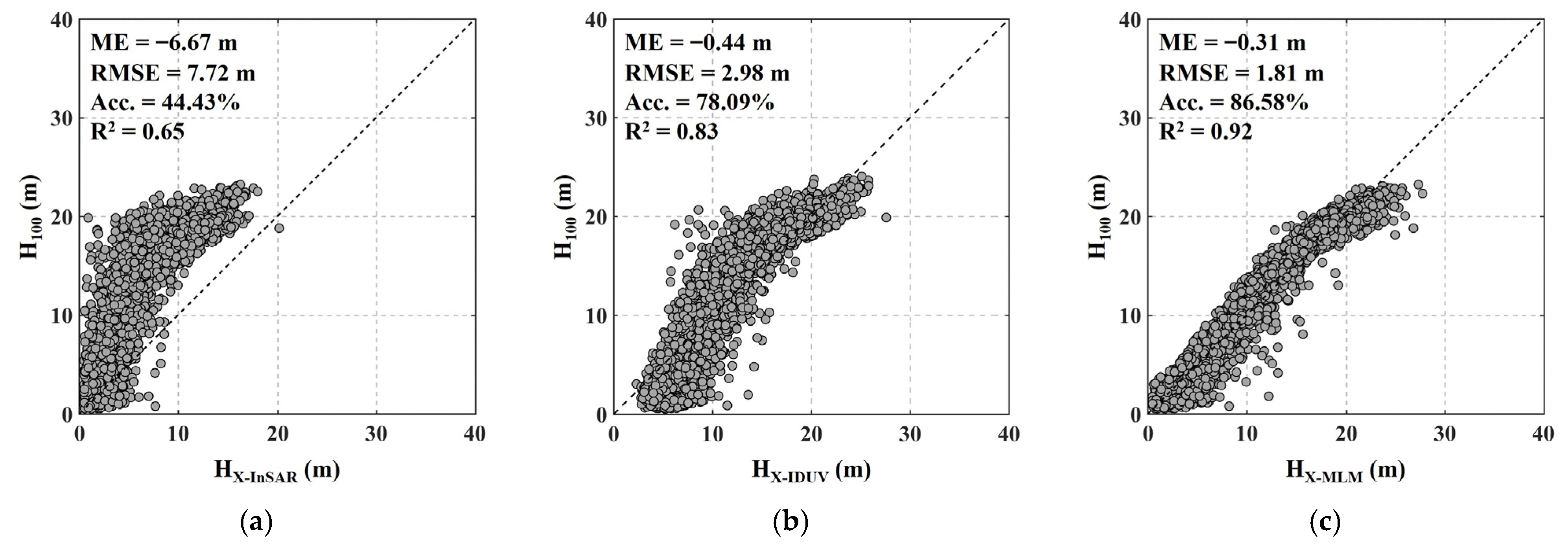
5.3. Estimation Results of Forest Height

For the sake of description, H_X-InSAR, H_X-IDUV and H_X-MLM were used to label the estimation results of the forest height generated based on DSM_X-InSAR, DSM_X-IDUV and DSM_X-MLM, respectively. The final estimation results of forest height are shown in Figure 16. Comparisons of the estimation results with H₁₀₀ (Figure 7d) revealed that overall forest height was underestimated in H_X-InSAR. In contrast, H_X-IDUV and H_X-MLM were obviously higher and closer to H₁₀₀ than H_X-InSAR. However, in H_X-IDUV, there were still some obvious deficiencies. For example, the underestimation was still observed in several forest-covered areas such as the northwest of the study area (marked by the black circle in Figure 16b,c), and the overestimation was observed in the bare soil/non-vegetated areas such as those in the southeast of the study area (marked by the red circle in Figure 16b,c). Overall, the best consistency was observed between H_X-MLM and H₁₀₀.

Based on the evaluation indicators (Table 1) and H₁₀₀ data (Figure 7d), the forest height estimation results were quantitatively evaluated. Figure 17a–c shows the scatter plots of H₁₀₀ with respect to H_X-InSAR, H_X-IDUV and H_X-MLM, respectively. The evaluation indicators of each forest height estimation result are also shown in the figure. It can be observed in Figure 17 that H_X-MLM achieved the most accurate forest height estimation result with an accuracy of 86.58%, which was 8.49% more accurate compared with H_X-IDUV and 42.15% more accurate compared with H_X-InSAR.

Similarly, for more detailed exhibition and analysis, the forest height profile in the same location as Figure 15 was extracted and is displayed in Figure 18. It can be seen that after removing the understory topography, the normalized forest height profile shows more and clearer details. Overall, consistent with the previous analysis, H_X-MLM showed the best agreement with H₁₀₀. That is, for tall forest areas, the method based on the MLM compensated better than the IDUV model. In the low vegetation areas (marked by the red circle in Figure 18) such as the area around 117°19′32.5″, both methods overestimated the height. Moreover, the overestimation phenomenon of H_X-MLM was obviously weaker.

There may be two reasons for the above-mentioned overestimation phenomenon. First, when comparing the LiDAR data of the test area (marked by red polygons in Figure 7c), it is not difficult to see that the overestimation phenomenon was basically located in the heterogeneous region, such as the edge of the forest. Owing to the characteristics of side-looking illumination by SAR sensors, the scatterer information of nearby tall trees was likely mixed in the non-vegetation pixels, resulting in overestimation (including H_X-InSAR). Second, the coherence observations (γ_IDUV and γ_MLM) still contained some non-forest-induced decoherence that was not removed. In addition, it should be noted that both methods had an obvious underestimation in some regions, such as the area around 117°20′10″. The main reason is that this area is a very sparse forest, and although the decoherence caused by the forest was small, H₁₀₀ still took the maximum value within the modeling unit. In other words, the scattering mechanisms were inconsistent with the model assumptions of IDUV and MLM.

6. Discussion

In this paper, we proposed a method for forest height estimation using the penetration difference between P-band and X-band InSAR. Although the experimental results verified the effectiveness of the proposed method, some key issues and future developments of this study should be further described.

For DTM extraction based on P-band InSAR, we adopted the improved TF analysis method proposed by Fu et al. [18], which used a subaperture decomposition technique to enhance the ability of P-band SAR to “see” the pure ground surface through forest gaps. In this paper, we again verified the effectiveness of the TF analysis method. However, it should be noted that the experimental verification of the TF method included in this study was based on the airborne P-band high-resolution InSAR data [17,18]. It is important to note that this method is only suitable for high-resolution long-wavelength InSAR data. However, this requirement is somewhat difficult for spaceborne long-wavelength SAR. For example, the spaceborne P-band InSAR mission BIOMASS will have a spatial resolution of about 12.5 m × 25 m [43], which is much lower than the spatial resolution of airborne InSAR data used in this study. Low spatial resolution will lead to a narrow observation angle. For this situation, it is also difficult to obtain pure ground surface SLC pixels with methods based on TF analysis. In other words, the size of the SLC pixel is likely to be larger than the forest gap that can be penetrated, and mixing in forest scatterers is unavoidable. In this case, it may be useful to consider the dielectric penetration scattering mechanism within the SLC pixel based on the TF analysis method. In addition to algorithmically adapting to low resolutions as much as possible, we strongly recommend launching the P-band SAR satellites with a spatial resolution better than 3 m to improve the gap penetration capability of spaceborne SAR. It is notable that China’s civil P-band SAR has just entered the pre-research stage, and higher spatial resolution should be the basic feature of this satellite [44]. In addition, the TF method only increases the probability of the SAR signal seeing the pure ground surface by changing the observation angle in the azimuth direction. In fact, in the range direction, the viewing angle of the SAR relative to the forest has a strong effect on the penetration ability. In general, a smaller angle of incidence is more conducive to penetration of the forest [9]. However, in this paper, the incident angle of the P-band SAR was about 63 degrees, which is relatively large. This may also have an impact on the extraction accuracy of the DTM. If multi-angle InSAR observations are carried out in the range direction, such as complementary observations of ascending and descending orbits, it will be possible to further increase the possibility of SAR sensors seeing the pure ground surface.

For DSM extraction based on X-band InSAR, we proposed a new compensation method based on the gap penetration scattering mechanism. Compared with the IDUV method, the advantage of our method is that there is no theoretical limit on the maximum penetration depth, so it is more likely to be applied to diverse forests. Because of the wavelength limitation, X-band cannot use subaperture decomposition technology to enhance the ability of gap penetration, like high-resolution P-band SAR. Even so, the gap penetration capability of the X-band is unquestionable. For example, Lei et al. realized the simultaneous automatic extraction of the DTM and DSM in the tropical forest area by using the gap penetration ability of the X-band InSAR [31]. However, in Lei’s method, in order to avoid the influence of multi-look averaging, only few looks can be performed. In this case, the algorithm must have strong adaptability to the influence of various noises. In contrast, we did not need to worry about this aspect with our method. Within an estimation unit (such as 20 m × 20 m), we did not focus on extracting the phase of the SLC pixel that has the highest phase center and is close to the location of the forest canopy top because the phase of a single SLC pixel has a large uncertainty. We chose to average all SLC pixels in the estimation unit to eliminate the influence of noise, and then reconstruct the position of the highest SLC pixel with certain model assumptions mainly about the distribution of the scatters. Therefore, for our method, reasonable model assumptions about the distribution of the scatters based on the type and structure of the specific forest are the most important for the extraction accuracy of DSM. In this study, the distribution was assumed to be uniform for the purpose of model simplicity. Obviously, this does not work for all forest types. For example, for sparse forest, the scatterers are more likely to be concentrated on the ground surface than be evenly distributed. In this case, a more complex and realistic distribution rather than uniform distribution may improve the extraction accuracy of the DSM, thereby improving the estimation accuracy of the forest height. As a previous study [28] shows, the MLM with a mixed truncated normal distribution achieved a superior forest height result compared to the model with less complex distribution. Further study will focus on the more complex scatters distribution to improve the accuracy and adaptability of the MLM-based DSM compensation method.

In addition, it should be mentioned that the integration of InSAR data from a different frequency requires accurate geo-positioning and comparable spatial resolution, especially when the data are obtained with a different platform. In our case, the spaceborne X-band InSAR data and airborne P-band InSAR data were used. Along with these data, accurate orbit information and image parameters were provided, which allowed us to perform accurate geocoding (within 1 pixel,) for both datasets based on the Range-Doppler positioning model. The resolutions of the airborne and spaceborne InSAR SLC data are comparable. Therefore, the influence of this aspect on the results of this paper should be small.

7. Conclusions

This paper presented a forest height estimation approach utilizing the penetration difference between P-band and X-band InSAR data. The forest height was determined by subtracting the P-band DTM from the X-band DSM. To realize the unbiased DTM extraction, the improved TF analysis method was utilized to separate and obtain the pure underlying topography phase. The method enhanced the capability of gap penetration of the P-band InSAR by adopting subaperture decomposition. To compensate for the height bias in the DSM, we proposed a novel method based on the MLM. As opposed to traditional scattering models (such as IDUV, RVoG), which focus on the dielectric penetration of the SAR signal, the MLM emphasizes the penetration capability of the radar, which is more in line with the characteristics of the scattering mechanism for X-band InSAR in a forest scenario.

Based on the spaceborne X-band and airborne P-band InSAR data of the Saihanba Forest Farm, the proposed method was validated. The experimental results showed that the extracted DTM based on the TF method achieved an RMSE with an accuracy of about 0.94 m, which is sufficient for forest height estimation. The proposed MLM-based DSM compensation method outperformed the IDUV-based method by 1.34 m in terms of RMSE. Furthermore, in the area where the original X-band DSM underestimated the forest surface height over 10 m, the MLM-based method achieved a better compensated result compared to the IDUV-based method. As a result, under the extracted P-band DTM, the forest height estimation based on the MLM-based compensation method achieved better accuracy (Acc. = 86.58%, RMSE = 1.81 m) compared to the IDUV-based method (Acc. = 78.09%, RMSE = 2.98 m). The results demonstrate the effectiveness of the proposed forest height estimation method in the study area. In the future, we plan to adopt this approach to estimate the forest height in more and larger areas to further assess the adaptability of the method.

References

- GCOS. The Global Observing System for Climate: Implementation Needs; Global Climate Observing System: Geneva, Switzerland, 2016. [Google Scholar]
- Sexton, J.O.; Bax, T.; Siqueira, P.; Swenson, J.J.; Hensley, S. A comparison of lidar, radar, and field measurements of canopy height in pine and hardwood forests of southeastern North America. For. Ecol. Manag. 2009, 257, 1136–1147. [Google Scholar] [CrossRef]
- Qi, W.; Saarela, S.; Armston, J.; Ståhl, G.; Dubayah, R. Forest biomass estimation over three distinct forest types using TanDEM-X InSAR data and simulated GEDI lidar data. Remote Sens. Environ. 2019, 232, 111283. [Google Scholar] [CrossRef]
- Tebaldini, S.; Rocca, F. Multibaseline polarimetric SAR tomography of a boreal forest at P-and L-bands. IEEE Trans. Geosci. Remote Sens. 2011, 50, 232–246. [Google Scholar] [CrossRef]
- Cloude, S. Polarisation: Applications in Remote Sensing; OUP Oxford: Oxford, UK, 2009. [Google Scholar]
- Aulinger, T.; Mette, T.; Papathanassion, K.; Hajnsek, I.; Heurich, M.; Krzystek, P. Validation of heights from interferometric SAR and LIDAR over the temperate forest site “Nationalpark Bayerischer Wald”. In Proceedings of the POLinSAR 2005 Workshop, Frascati, Italy, 17–21 January 2005; p. 11. [Google Scholar]
- Andersen, H.-E.; McGaughey, R.; Reutebuch, S.; Schreudera, G.; Agee, J.; Mercer, B. Estimating canopy fuel parameters in a Pacific Northwest conifer forest using multifrequency polarimetric IFSAR. Image 2004, 900, 74. [Google Scholar]
- Santos, J.; Neeff, T.; Dutra, L.; Araujo, L.; Gama, F.; Elmiro, M. Tropical forest biomass mapping from dual frequency SAR interferometry (X and P-Bands). ISPRS Int. Soc. Photogramm. Remote Sens. Tech. Comm. VII 2004, 35, 1682–1777. [Google Scholar]
- Shiroma, G.H.X.; de Macedo, K.A.C.; Wimmer, C.; Moreira, J.R.; Fernandes, D. The dual-band PolInSAR method for forest parametrization. IEEE J. Sel. Top. Appl. Earth Obs. Remote Sens. 2016, 9, 3189–3201. [Google Scholar] [CrossRef]
- Balzter, H.; Rowland, C.S.; Saich, P. Forest canopy height and carbon estimation at Monks Wood National Nature Reserve, UK, using dual-wavelength SAR interferometry. Remote Sens. Environ. 2007, 108, 224–239. [Google Scholar] [CrossRef]
- Karamvasis, K.; Karathanassi, V. Forest canopy height estimation using double-frequency repeat pass interferometry. In Proceedings of the Third International Conference on Remote Sensing and Geoinformation of the Environment (RSCy2015), Paphos, Cyprus, 16–19 March 2015; pp. 132–141. [Google Scholar]
- Kugler, F.; Schulze, D.; Hajnsek, I.; Pretzsch, H.; Papathanassiou, K.P. TanDEM-X Pol-InSAR performance for forest height estimation. IEEE Trans. Geosci. Remote Sens. 2014, 52, 6404–6422. [Google Scholar] [CrossRef]
- Xie, Y.; Zhu, J.; Fu, H.; Wang, C. A review of underlying topography estimation over forest areas by InSAR: Theory, advances, challenges and perspectives. J. Cent. South Univ. 2020, 27, 997–1011. [Google Scholar] [CrossRef]
- Rignot, E. Dual-frequency interferometric SAR observations of a tropical rain-forest. Geophys. Res. Lett. 1996, 23, 993–996. [Google Scholar] [CrossRef] [Green Version]
- Mercer, B.; Zhang, Q.; Schwaebisch, M.; Denbina, M.; Cloude, S. Forest height and ground topography at L-band from an experimental single-pass airborne Pol-InSAR system. In Proceedings of the POLinSAR 2009, Frascati, Italy, 26–31 January 2009. [Google Scholar]
- Liao, Z.; He, B.; van Dijk, A.I.; Bai, X.; Quan, X. The impacts of spatial baseline on forest canopy height model and digital terrain model retrieval using P-band PolInSAR data. Remote Sens. Environ. 2018, 210, 403–421. [Google Scholar] [CrossRef]
- Garestier, F.; Dubois-Fernandez, P.C.; Champion, I. Forest height inversion using high-resolution P-band Pol-InSAR data. IEEE Trans. Geosci. Remote Sens. 2008, 46, 3544–3559. [Google Scholar] [CrossRef]
- Fu, H.; Zhu, J.; Wang, C.; Wang, H.; Zhao, R. Underlying topography estimation over forest areas using high-resolution P-band single-baseline PolInSAR data. Remote Sens. 2017, 9, 363. [Google Scholar] [CrossRef] [Green Version]
- Treuhaft, R.N.; Siqueira, P.R. Vertical structure of vegetated land surfaces from interferometric and polarimetric radar. Radio Sci. 2000, 35, 141–177. [Google Scholar] [CrossRef] [Green Version]
- Su, Y.; Guo, Q. A practical method for SRTM DEM correction over vegetated mountain areas. ISPRS J. Photogramm. Remote Sens. 2014, 87, 216–228. [Google Scholar] [CrossRef]
- Schlund, M.; Baron, D.; Magdon, P.; Erasmi, S. Canopy penetration depth estimation with TanDEM-X and its compensation in temperate forests. ISPRS J. Photogramm. Remote Sens. 2019, 147, 232–241. [Google Scholar] [CrossRef]
- Ni, W.; Guo, Z.; Sun, G.; Chi, H. Investigation of forest height retrieval using SRTM-DEM and ASTER-GDEM. In Proceedings of the 2010 IEEE International Geoscience and Remote Sensing Symposium, Honolulu, HI, USA, 25–30 July 2010; pp. 2111–2114. [Google Scholar]
- Ni, W.; Zhang, Z.; Sun, G.; Guo, Z.; He, Y. The penetration depth derived from the synthesis of ALOS/PALSAR InSAR data and ASTER GDEM for the mapping of forest biomass. Remote Sens. 2014, 6, 7303–7319. [Google Scholar] [CrossRef] [Green Version]
- Solberg, S.; May, J.; Bogren, W.; Breidenbach, J.; Torp, T.; Gizachew, B. Interferometric SAR DEMs for forest change in Uganda 2000–2012. Remote Sens. 2018, 10, 228. [Google Scholar] [CrossRef] [Green Version]
- Dall, J. InSAR elevation bias caused by penetration into uniform volumes. IEEE Trans. Geosci. Remote Sens. 2007, 45, 2319–2324. [Google Scholar] [CrossRef] [Green Version]
- De Zan, F.; Krieger, G.; López-Dekker, P. On some spectral properties of TanDEM-X interferograms over forested areas. IEEE Geosci. Remote Sens. Lett. 2012, 10, 71–75. [Google Scholar] [CrossRef] [Green Version]
- Soja, M.J.; Ulander, L.M. Two-level forest model inversion of interferometric TanDEM-X data. In Proceedings of the EUSAR 2014, 10th European Conference on Synthetic Aperture Radar, Berlin, Germany, 3–5 June 2014; pp. 1–4. [Google Scholar]
- Zhao, L.; Chen, E.; Li, Z.; Zhang, W.; Fan, Y. A New Approach for Forest Height Inversion Using X-Band Single-Pass InSAR Coherence Data. IEEE Trans. Geosci. Remote Sens. 2021, 60, 1–18. [Google Scholar] [CrossRef]
- Soja, M.J.; Persson, H.; Ulander, L.M. Estimation of forest height and canopy density from a single InSAR correlation coefficient. IEEE Geosci. Remote Sens. Lett. 2014, 12, 646–650. [Google Scholar] [CrossRef] [Green Version]
- Soja, M.J.; Persson, H.J.; Ulander, L.M. Detection of forest change and robust estimation of forest height from two-level model inversion of multi-temporal, single-pass InSAR data. In Proceedings of the 2015 IEEE International Geoscience and Remote Sensing Symposium (IGARSS), Milan, Italy, 26–31 July 2015; pp. 3886–3889. [Google Scholar]
- Lei, Y.; Treuhaft, R.; Gonçalves, F. Automated estimation of forest height and underlying topography over a Brazilian tropical forest with single-baseline single-polarization TanDEM-X SAR interferometry. Remote Sens. Environ. 2021, 252, 112132. [Google Scholar] [CrossRef]
- Garestier, F.; Dubois-Fernandez, P.C.; Papathanassiou, K.P. Pine forest height inversion using single-pass X-band PolInSAR data. IEEE Trans. Geosci. Remote Sens. 2007, 46, 59–68. [Google Scholar] [CrossRef]
- Ferro-Famil, L.; Reigber, A.; Pottier, E. Scene characterization using sub-aperture polarimetric interferometric SAR data. In Proceedings of the IGARSS 2003. 2003 IEEE International Geoscience and Remote Sensing Symposium, Toulouse, France, 21–25 July 2003; pp. 702–704. [Google Scholar]
- Singh, J.; Datcu, M. SAR target analysis based on multiple-sublook decomposition: A visual exploration approach. IEEE Geosci. Remote Sens. Lett. 2011, 9, 247–251. [Google Scholar] [CrossRef]
- Moreira, A. Real-time synthetic aperture radar(SAR) processing with a new subaperture approach. IEEE Trans. Geosci. Remote Sens. 1992, 30, 714–722. [Google Scholar] [CrossRef]
- Small, D. Generation of Digital Elevation Models through Spaceborne SAR Interferometry; University of Zurich: Zurich, Switzerland, 1998. [Google Scholar]
- Richards, J.A. Remote Sensing with Imaging Radar; Springer: Berlin/Heidelberg, Germany, 2009; Volume 1. [Google Scholar]
- Pang, Y.; Li, Z.; Ju, H.; Lu, H.; Jia, W.; Si, L.; Guo, Y.; Liu, Q.; Li, S.; Liu, L. LiCHy: The CAF’s LiDAR, CCD and hyperspectral integrated airborne observation system. Remote Sens. 2016, 8, 398. [Google Scholar] [CrossRef] [Green Version]
- Pang, Y.; Liang, X.; Jia, W.; Si, L.; Yan, G.; Shi, J. The comprehensive airborne remote sensing experiment in Saihanba forest farm. J. Remote Sens. 2021, 25, 14. [Google Scholar]
- Li, Z.; Ding, X.; Huang, C.; Zhu, J.; Chen, Y. Improved filtering parameter determination for the Goldstein radar interferogram filter. ISPRS J. Photogramm. Remote Sens. 2008, 63, 621–634. [Google Scholar] [CrossRef]
- Chen, C.W.; Zebker, H.A. Two-dimensional phase unwrapping with use of statistical models for cost functions in nonlinear optimization. JOSA A 2001, 18, 338–351. [Google Scholar] [CrossRef] [Green Version]
- Krieger, G.; Moreira, A.; Fiedler, H.; Hajnsek, I.; Werner, M.; Younis, M.; Zink, M. TanDEM-X: A satellite formation for high-resolution SAR interferometry. IEEE Trans. Geosci. Remote Sens. 2007, 45, 3317–3341. [Google Scholar] [CrossRef] [Green Version]
- Minh, D.H.T.; Le Toan, T.; Rocca, F.; Tebaldini, S.; Villard, L.; Réjou-Méchain, M.; Phillips, O.L.; Feldpausch, T.R.; Dubois-Fernandez, P.; Scipal, K. SAR tomography for the retrieval of forest biomass and height: Cross-validation at two tropical forest sites in French Guiana. Remote Sens. Environ. 2016, 175, 138–147. [Google Scholar] [CrossRef] [Green Version]
- Li, W.; Tong, Q.; Xu, L.; Ji, P.; Dong, F.; Yu, Y.; Chen, J.; Zhao, L.; Zhang, L.; Xie, C. The P-band SAR Satellite: Opportunities and Challenges. In Proceedings of the 2019 6th Asia-Pacific Conference on Synthetic Aperture Radar (APSAR), Xiamen, China, 26–29 November 2019; pp. 1–6. [Google Scholar]