Mapping Plant Species in a Former Industrial Site Using Airborne Hyperspectral and Time Series of Sentinel-2 Data Sets

Abstract

Industrial activities induce various impacts on ecosystems that influence species richness and distribution. An effective way to assess the resulting impacts on biodiversity lies in vegetation mapping. Species classification achieved through supervised machine learning algorithms at the pixel level has shown promising results using hyperspectral images and multispectral, multitemporal images. This study aims to determine whether airborne hyperspectral images with a high spatial resolution or phenological information obtained by spaceborne multispectral time series (Sentinel-2) are suitable to discriminate species and assess biodiversity in a complex impacted context. The industrial heritage of the study site has indeed induced high spatial heterogeneity in terms of stressors and species over a reduced scale. First, vegetation indices, derivative spectra, continuum removed spectra, and components provided by three feature extraction techniques, namely, Principal Component Analysis, Minimal Noise Fraction, and Independent Component Analysis, were calculated from reflectance spectra. These features were then analyzed through Sequential Floating Feature Selection. Supervised classification was finally performed using various machine learning algorithms (Random Forest, Support Vector Machines, and Regularized Logistic Regression) considering a probability-based rejection approach. Biodiversity metrics were derived from resulted maps and analyzed considering the impacts. Average Overall Accuracy (AOA) reached up to 94% using the hyperspectral image and Regularized Logistic Regression algorithm, whereas the time series of multispectral images never exceeded 72% AOA. From all tested spectral transformations, only vegetation indices applied to the time series of multispectral images increased the performance. The results obtained with the hyperspectral image degraded to the specifications of Sentinel-2 emphasize the importance of fine spatial and spectral resolutions to achieve accurate mapping in this complex context. While no significant difference was found between impacted and reference sites through biodiversity metrics, vegetation mapping highlighted some differences in species distribution.

1. Introduction

Industrial processing, agriculture, mining, transportation, and urban development are intensively growing as the human population increases [1,2,3]. Since anthropogenic activities can result in several environmental impacts, being able to monitor them through remote sensing is of primary importance [1,4]. At least three United Nations Sustainable Development Goals (SDGs) are directly concerned with these problems [5]: the objective “zero hunger”, which focuses on food and agriculture security; the objective “clean water and sanitation”, which searches to ensure availability and sustainable management of water and sanitation for all; and the “life on land” objective, aiming to protect ecosystems and biodiversity.

In particular, anthropogenic impacts on soil could be declined in those linked to soil chemical compounds and reactions (chemical impacts) and those linked to soil structure, texture, and compaction (physical impacts) [6]. As plants are rooted in soils, they can be used as an indirect indicator of such impacts. Changes in soil physical properties can lead to negative effects on root growth, nutrient availability, air permeability, and water-holding capacities and transport [7,8]. Chemical impacts result from soil contamination, such as hydrocarbon or heavy metal contamination, and fertilization. Both are known to be interlinked and influence vegetation health by affecting soil productivity and fertility [6,9]. It turns out that species differ in their sensitivity to various impacts [10,11,12]. In addition, studies have shown that knowing the sensitivity of a given species to a given stressor, the stress level, or possibly the stressor itself can be detected or even quantified through vegetation health [13,14,15]. In the context of several anthropogenic impacts, distinguishing several stressors could be achieved by exploiting those differences in sensitivity [4]. Some species present a lower biomass and higher mortality rate in the context of impacted soil properties [13,14]. Conversely, other species, such as plant metallophytes, are known to be resistant to certain impacts and serve as indicator species of impacted soils [15]. These effects lead to changes in species richness and spatial distribution within an ecosystem [15,16,17,18]. Thus, being able to map vegetation in the context of multiple anthropogenic impacts is crucial to either assess biodiversity, identify species composition and its changes over time, and is an essential preliminary step to detect, characterize, and quantify plant stressors.

Since they provide rapid and non-destructive acquisitions in a wide field, remote sensing instruments have been increasingly investigated for vegetation mapping and biodiversity assessment. Indeed, passive optical sensors can provide surface spectral reflectance of spectral bands linked to plant properties or species-specific characteristics [19,20,21,22]. Used in conjunction with supervised classification algorithms, based on class-specific information provided by training samples, both hyperspectral and multispectral images have been proved to be particularly suitable [23]. Nevertheless, few or no studies have been conducted focused on species mapping in the context of anthropogenic influence on soils. In such a context, classifications have generally applied to discriminate stressed from non-stressed vegetation rather than species [24,25,26] or have been conducted at an in situ scale [11]. Yet, stressors bring an additional challenge to reach accurate species classification since their presence has repercussions on plant spectral reflectance [10,11,27,28]. The intraspecific variability (spectral variations observed within species) results mainly from species’ inherent factors (such as phenology stage and plant age) and is related to environmental conditions (such as soil characteristics, topography, exposition, and weather conditions). The presence of stressors increases this variability, causing classification errors [6,29]. In addition to this challenge, impacted sites are often small areas with high spatial heterogeneity (within soil and species) and are sometimes species too poorly represented to be included in the training base for supervised approaches.

Another key issue in the context of anthropogenic impacts lies in the quantitative assessment of biodiversity through biodiversity metrics [30], which are proven to be correlated to species richness and anthropogenic impacts [27]. Most quantitative assessments of biodiversity from remote sensing rely on the spectral variation hypothesis, which assumes a relationship between the spectral heterogeneity of the data and species richness [31]. However, this assumption is particularly delicate when intraspecific variability is high [32]. Working in the context of anthropogenic impacts requires specific methods.

In a more global context, hyperspectral data allowed distinguishing subtle differences in reflectance among species at high (metric) to moderate (decametric) spatial resolutions according to homogenous vegetation patch size [28,31]. Most studies involved mapping forest-tree species (around 10 species) [33,34,35,36,37,38,39]. Yet, these hyperspectral data exploitations also allowed us to analyze heterogeneous ecosystems, such as alkali landscapes [40] or aquatic vegetation [41].

Satellite multispectral imagery permitted us to reach performances similar to those conducted with single-date hyperspectral imagery in various contexts. The main advantage of satellite imagery lies in its availability and revisit frequency since it gives access to vegetation phenology. Previous studies showed that performance changes according to the number of dates exploited and the phenological stages considered. For instance, Hill et al. noticed that broadleaf species in a temperate area are better discriminated in spring (flowering season) and autumn (senescence season) [42]. Several studies exploiting multitemporal imagery confirmed this observation by reporting an increase in classification accuracy regardless of the vegetation type [30,31,32].

The time series of multispectral images could achieve a similar or even slightly better performance than single-date hyperspectral imagery for similar spatial resolutions applied to forest-tree species classifications [43,44,45]. However, satellite instruments, mandatory to obtain high revisit frequencies, provide lower spatial resolutions than airborne ones. Using a coarser spatial resolution does not necessarily decrease the classification performance since it may reduce intraspecific variability [46]. Nevertheless, such resolutions lead studies to be conducted over relatively large areas (around 10 to 1000 km²) to obtain sufficient pure pixels for supervised classification. While such area sizes are common for forest-tree species classifications, other contexts may prevent such extents. The spatial resolution reached by airborne instruments could therefore be mandatory.

Whatever the type of remote sensing data is considered, studies have shown that machine learning algorithms are well-suited for solving supervised classification problems [23,46,47]. Two types of classification algorithms can be declined: parametric algorithms, underlying an assumption on feature distribution, and non-parametric algorithms without a priori hypothesis. Both have proved efficient in solving vegetation classification problems [46,47]. Nonetheless, since parametric algorithms assume that features are normally distributed, which is rarely observed in remote sensing data [48,49], non-parametric algorithms, especially Support Vector Machines and Random Forest, are the most widespread algorithms. Moreover, they are able to handle the high dimensionality of input features [46]. These algorithms were successfully applied to various classification problems, including tree species [37,38,40,50,51], shrubs, and herbaceous vegetation mapping [40,52,53].

Although a strong performance is obtained using reflectance spectra [37], feature transformations (e.g., derivations, continuum removal, and spectral indices) are almost inherent to hyperspectral-based classification [46,47,54]. Common transformations resulted in inconsistent performance on tree species classification [39,46,55]. However, they emphasized that enhancing the spectral information was crucial to better distinguish certain species. For example, these transformations improved both peatland species classifications using field hyperspectral data and assemblages of grass species based on satellite multispectral images [52,53]. Moreover, when combined with feature reduction, feature transformation may reduce feature correlation and limit overfitting. Data with high dimensionality are indeed prone to Hughes’ phenomenon, according to which too many input features lead to a decline in performance [37,54,56,57].

Two kinds of feature reduction methods are generally exploited: feature selection and extraction [46]. The former selects a subset of features based on specific criteria, revealing spectral regions with high discriminatory power. An example lies in regularization penalties implanted in Regularized Logistic Regression (RLR) [58]. This technique is often used to reduce feature number [59,60] and proved efficient for the classification of complex species using hyperspectral data [52,61]. Selection methods can also be considered as a distinct stage from the classification algorithm, as done in the Sequential Floating Feature Selection (SFFS) [37,62]. Feature extraction is based on the computation of new predictor variables, making difficult their interpretation but often allowing the best performance [34,46]. In this category, dimension reduction techniques are widespread in remote sensing. The Principal Component Analysis (PCA) and its derivatives, the kernel PCA or the Minimum Noise Fraction (MNF), or the Independent Component Analysis (ICA) have indeed proven their utility in vegetation classification [34,35,40,63]. The performance reached with different feature reduction methods depends on several parameters including signal-to-noise ratio, data characteristics, study context (classification level, class number, pixel or object-based approach, …), and classification algorithm [64]. As an example, Torabzadeh et al. obtained better results with SFFS than PCA at the tree level while Fassnacht et al. found the MNF greater than three feature selection techniques [34,62]. Several transformations and feature reduction methods should thus be applied to assess their classification performance improvement in a specific context.

Few works addressing under-represented classes have focused on rejection methods. Such methods aim to identify the most uncertain classifications. A possible way to do that consists of adding contextual, often spatial, information [65]. Such approaches ask for a classification algorithm able to deduce contextual knowledge from data. The second way to determine uncertain predictions consists of using thresholds on the prediction probabilities [66]. To our knowledge, none of these methods have already been tested on natural vegetation. Thus, a method associated with the prediction probabilities of algorithms proven effective for remote sensing species classification problems seems more appropriate to define a classification method efficient in particularly complex sites.

The objective of this study consists of mapping vegetation species and assessing biodiversity on a particularly complex site characterized by different vegetation units exposed to multiple stressors, including soil contamination. This could help to define a reference method in the context of anthropogenic impacts at the local scale. This method could then be used directly to identify impact-sensitive species and monitor the state of exposed vegetation, and as a preliminary step to detect, characterize, and quantify plant stressors. To that aim, supervised classification based on metric hyperspectral images and time series of decametric multispectral images are compared and extended to (i) map vegetation species across an industrial site, (ii) consider under-represented species within mapping through a rejection method, and (iii) assess biodiversity metrics across an industrial site directly from vegetation mapping.

2. Materials

2.1. Study Site

The study site was an industrial brownfield extending over 2.45 km² in a temperate oceanic region with a warm summer but no dry season (Figure 1). The average annual temperature was about 14 °C, with a difference of 18 °C between the lowest and the highest average monthly temperatures in 2017. A total of 1032 mm of rain fell this year (range of 115 mm between the driest and wettest months). The site corresponded to a former flood expansion and included wetlands. It was located on recent alluvium. A tertiary molasses bedrock considered impermeable underlay these alluviums. The local vegetation was dominated by a deciduous riparian forest with various successional stages. Part of the site, here called the impacted site, had been exposed to extensive oil, gas, and other industrial activities for approximately 50 years. These activities resulted in several impacts on soil properties, including chemical contamination (heavy metals and petroleum hydrocarbons [25,67]) and physical transformations (rubble and pipe burying). These impacts were clustered around different locations depending on the history of the site. Nevertheless, the entire site was impacted. Native tree, shrubby, and grassland vegetation heterogeneously distributed had recolonized the site over time. The second part of the site, called the reference site, presented the same species and assemblages but with no chemical impacts on soils. In addition to natural species, crops, mainly corn crops, were scattered on both sites. These agricultural parcels were already present before any industrial activity and their exploitation had continued since. Except for crops and a poplar grove in the northwest of the reference site, human beings introduced no vegetation.

2.2. Species Inventory

Two species inventories were conducted in the field, in November 2020 (senescence period for deciduous species) and July 2021 (summer), to identify the predominant genera and species within the sites (

Table 1. Predominant genera and species descriptions.

Genus/Assemblage of Genera	Species	Tree Crowns or Sample Units (Sample Unit: Homogeneous Area Manually Delineated) (n)
Platanus	sp.	28
Salix	cinerea, babylonica	42
Populus	nigra, alba	35
Quercus	pubescens, robur	37
Fraxinus	excelsior	17
Acer	campestre	7
Alnus	glutinosa	61
Ulmus	minor	5
Robinia	pseudoacacia	46
Castanea	sativa.	1
Juglans	nigra, regia	3
Corylus	avellana	18
Reynoutria	japonica	21
Shrub mixtures	Rubus fruticosus, Cornus sanguinea, Buddleja davidii	30
Grass mixtures	Mix of various grasses and dicots	15

). Some genera were only found intertwined with each other. Since it was not possible to distinguish them at a metric spatial resolution, these genera were merged in assemblages of genera (grass or shrub mixtures). The locations of individual trees and homogenous areas were recorded using a GPS-RTK (precision around one centimeter). A database was created from these inventories in a Geographic Information System (GIS) and completed by photointerpretation. For each sampled point, the corresponding tree crowns and homogeneous herbaceous/shrubby areas were manually delineated using the 20 cm BD ORTHO^® provided by the French National Geographic Institute (IGN, [68]). Pixels at the edges of the crown were avoided as they might correspond to intersections between different tree canopies. Each delineated sample was defined as a unit in the next. To ensure sufficient reference data, classes were defined at the genus or assemblage level. A total of 15 classes corresponding to genera (either monospecific or plurispecific on the study sites) were defined (Table 1). Knowing that crops were likely to vary over the time series, this class was kept only for the hyperspectral case.

2.3. Remote Sensing Imagery

2.3.1. Hyperspectral Imagery

Radiance hyperspectral images were provided by two airborne HySpex Cameras (Norsk Elektro Optikk AS, Lørenskog, Norway) on 5 July 2017 under a clear sky. The first camera was a HySpex VNIR-1600, which covered the Visible-Near-InfraRed domain (VNIR: 400–1000 nm) at a spectral resolution of 5.2 nm and spatial resolution of 1 m at 2000 m above ground. The second camera was an SWIR-230m-e covering the Short-Wave-InfraRed domain (SWIR: 1000–2500 nm) with a 7.8 nm spectral resolution and 2.5 m spatial resolution. The SWIR hypercube was co-registered with the VNIR hypercube using the Gefolki algorithm [69]. Both hypercubes were resampled to 1 m spatial resolution with a nearest neighborhood filter to preserve spectral information.

The atmospheric correction was provided by the Empirical Line Method (ELM) to obtain a reflectance hypercube at the ground level covering the reflective domain. The lack of information about the local industrial atmosphere composition (aerosol type and concentration) prevented the use of transfer radiative models. To improve the signal-to-noise ratio, a Savitzky–Golay filter was applied and spectral bands with low atmospheric transmission (<80%) were removed [52].

2.3.2. Multispectral Time Series

Sentinel-2 multispectral images covering the VNIR-SWIR domain were acquired by the Theia-Copernicus program [70]. Georeferenced reflectance images (level 2A) acquired in 2017 (the same year of the hyperspectral image data acquisition) over the study site were retained. A time series of Sentinel-2 images made of 32 dates was built after discarding cloudy images (Figure 2). Only spectral bands with spatial resolutions of 10 and 20 m were kept, and 20 m resolution bands were resampled to 10 m using a nearest neighborhood resampling filter.

3. Method Description

3.1. Preprocessing: Non-Vegetation and Shadow Masking

Sunlit vegetation pixels were located by combining several masks based on spectral indices [71]. Normalized Built-up Area Index (NBAI) and Band Ratio for Built-up Area (BRBA) were used to remove built pixels [72,73]. Water pixels were identified using the Normalized Difference Water Index (NDWI) and modified Normalized Difference Water Index (mNDWI) [74]. Soil-Adjusted Vegetation Index (SAVI) and Dry Bareness Spectral Index (DBSI) were applied to extract bare soil pixels [75,76]. In addition, the Normalized Difference Vegetation Index (NDVI) was computed to discard the remaining non-vegetation pixels [77]. Shadow detection was finally performed using the method proposed by Nagao et al. [78]. Thresholds were defined using Otsu’s algorithm [79]. This way, sunlit vegetation masks were generated for each Sentinel-2 image forming the time series and for the airborne hyperspectral image. This resulted, for instance, in a total of 11% of masked pixels in the hyperspectral image.

3.2. Supervised Classification

3.2.1. Reference Data

Three datasets were built from the species inventory (Section 2.2) and image products. The first one included pure pixels at a spatial resolution of 1 m (hyperspectral spatial resolution), the second at 10 m, and the last at 20 m (Sentinel-2 VNIR and SWIR native resolutions, respectively). The number of per-class pixels after preprocessing is described in

Table 2. Predominant plant genera or assemblages, and corresponding pixel numbers on hyperspectral and Sentinel-2 images. The classes finally selected in the classification are indicated by an asterisk.

Genus/Assemblage of Genera	HySpex Image	Sentinel-2 VNIR
Platanus *	4183	21
Salix *	1512	21
Populus *	2251	22
Quercus *	2936	20
Fraxinus	931	9
Acer	403	0
Alnus *	1588	20
Ulmus	305	0
Robinia *	1536	20
Castanea	107	0
Juglans	140	0
Corylus	40	0
Reynoutria *	1533	22
Shrub mixtures *	1944	19

. Only classes with sufficient samples were retained to avoid unbalance among classes (Table 2). A common rule in classification suggests having 10 times more samples than features [38]. Additionally, previous studies have shown that performance can be compromised in case of a high-class imbalance (e.g., 100:1), especially with a small sample size [80]. These conditions were met in our case of hyperspectral image processing. For Sentinel-2 imagery, the difficulty of obtaining pure pixels led to a low number of per-class samples. Since using a 20 m resolution database led to a very limited number of samples, only the VNIR database was conserved to perform classification with the 10 m spectral band of Sentinel-2 images covering the VNIR domain.

3.2.2. Data Splitting Procedure

Training and testing sets were created at the crown or sampling unit level to reduce spatial autocorrelation [81]. Indeed, spatial autocorrelation leads to biased performance evaluations of classification methods [46,47,81,82]. Our data were split according to the following schema: 50% of the labeled units were randomly selected in a stratified fashion for training, while the remaining 50% were kept for evaluation. Since a random selection was applied, the procedure was repeated iteratively 10 times [36,46,83].

3.2.3. Classification Principle

The flowchart describing the classification process is presented in Figure 3. Several methods used in previous studies were investigated and detailed in the following sections [52,61].

3.2.4. Feature Generation

Spectral Features

Since the vegetation at the site was composed of several genera and vegetation units (grasses, shrubs, and trees), various common spectral features were derived from reflectance spectra to identify the most appropriate for the studied context:

• Reflectance spectra;
• Spectral transformations linked to absorption features [52]:

  ○

  Continuum removal;

  ○

  First derivative;

• Spectral indices related to vegetation properties and biophysical parameters [84]:

  ○

  Narrowband vegetation indices, formulating simple ratio or normalized difference [47,69,82];

  ○

  Spectral positions (e.g., Red-edge Inflexion Point, REIP) [47,82];

  ○

  Spectral derivates (e.g., Edge-Green First derivative Ratio, EGFR) [47,82].

The notations and formulas proposed by Erudel et al. [52,85] and Fabre et al. [71] in previous work were retained, leading to a total of 176 indices. For the Sentinel-2 formulation, only indices derived from VNIR bands were considered (29 indices).

• Feature extractions [47]:

  ○

  Principal Component Analysis (PCA) [35];

  ○

  Minimal Noise Fraction (MNF), which removes the noise before applying PCA;

  ○

  Independent Component Analysis (ICA), which linearly projects the data onto a lower-dimensional space, non-orthogonal, so that the new components are as statistically independent as possible.

In the following parts, the $X^{th}$ components of the PCA, MNF, and ICA are, respectively, noted as PCAX, MNFX, and ICAX.

Temporal Features

Concerning multispectral images, the temporal behavior of the spectral features was considered via the dates composing the time series. The following scenarios were processed:

• Monthly series: one date per month;
• Seasonal series: one date per season;
• Entire time series: all the available dates defined in Section 2.2;
• Selection of key dates by SFFS (see Section 3.2.5).

Different statistics and distances were calculated in each temporal scenario to obtain the most discriminative compositions. For each class, the spectra of mean reflectance, spectra of median reflectance, mean spectra and median spectra, and associated standard deviation were generated. Two distances, Euclidean and Canberra, were then computed from those statistics. The temporal evolution of those statistics and distances were finally considered.

3.2.5. Feature Selection by Sequential Forward Feature Selection (SFFS)

SFFS is a sequential algorithm independent of the classifier used. A progressive search was conducted using a criterion to construct an ideal set of features [37]. According to the previous works, the separability criterion chosen was a measure commonly adopted in the literature; the Hellinger distance (also known as the Jeffries–Matusita distance) [37,52] defined as:

$$H\left(p,q\right)=\sqrt{\frac{1}{2}{\displaystyle \sum }_{i=1}^n{\left(\sqrt{p_i}-\sqrt{q_i}\right)}^2}$$

(1)

where $p$ and $q$ are the discrete distributions of each feature values of each class, and $n$ is the partition number. This distance indicates a total separability of two classes (described by their distributions) when its value is one.

3.2.6. Supervised Classification

All classification algorithms were performed using Python’s scikit-learn package (version 1.0.2) [86]. Corresponding parameters were optimized using 10-fold cross-validation across the training set.

Random Forest (RF)

RF is a non-parametric (distribution-free) ensemble algorithm based on decision trees [87]. The main advantages of this algorithm are its flexibility and non-sensitivity to noise [47]. It needs to initialize some parameters described hereafter. Here, the Gini Index, also known as Gini impurity, was exploited as a decision criterion. The number of trees was set at {100, 200, 500, 1000, 2000, 5000}. Correlation within the forest was reduced with a feature selection performed within a tree by randomly selecting $\sqrt{n}$ features and a maximum depth of trees varying between {2, 3, 5, 10, 15, 20, 25, 30, 40}.

Support Vector Machines (SVMs)

An SVM is a non-parametric classifier based on the construction of a hyperplane to separate data [88]. Since an SVM is initially defined for binary problems, a one-versus-rest (OVR) strategy was adopted to manage our number of classes. The advantages of this algorithm are the convexity of its cost function (an optimum solution is always provided) and its efficiency, even in the case of a low ratio between the number of training samples and the feature number [37,47]. It needs to fix some input parameters, as described bellow. Several values of hyperparameter C, called regularization strength, used in the optimization process were tested: C ∈ {1, 10, 100, 500, 1000, 5000, 10,000}. Two classical kernels, the linear and Radial Based Function (RBF), were computed. Their shape was defined by another hyperparameter γ, called the kernel size, for which the following values were tested: γ ∈ {0.0001, 0.001, 0.01, 0.1, 1}.

Regularized Logistic Regression (RLR)

RLR is a semi-parametric algorithm based on logistic regression improved by an additional regularization term called the penalty. Two classical penalties used as a feature selection method in remote sensing problems were retained [59,60]: the Lasso penalty, or ℓ1 regularization, incorporating a selection of features, and the Ridge regression, or ℓ2 regularized logistic regression, handling their collinearity. The regularization strength was controlled by hyperparameter C chosen in values ranging from C ∈ {0.01, 0.1, 1, 5, 10, 50, 100, 500, 1000, 5000}. While the RF and SVM are known as state-of-the-art algorithms [46], the few studies investigating RLR have proved its efficiency in species identification from hyperspectral data [25,52,61].

3.2.7. Performance Assessment

Average Overall Accuracy (AOA) and corresponding standard deviation were reported based on ten iterations. The evaluation was then performed using common metrics, namely, the confusion matrix and its associated metrics [48,89]. While Overall Accuracy (OA), and thus AOA, provides an overview of the obtained performance, the User’s Accuracy (UA), Producer’s Accuracy (PA), and F1-score (harmonic mean between UA and PA) allow a by-class analysis.

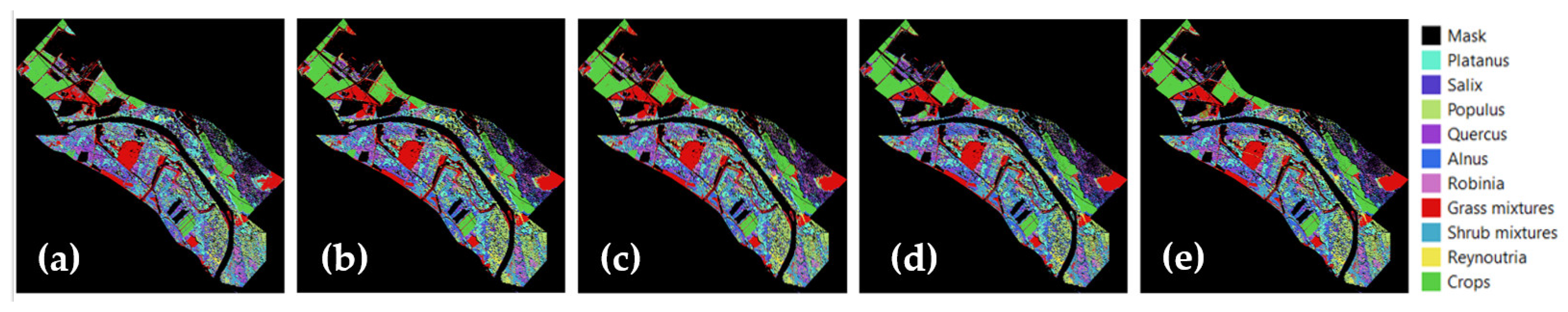
3.2.8. Species Map Generation and Rejection Class Definition

A mapping of genera/assemblages was produced over the entire site using the best-performing models. A majority-vote rule across iterations was adopted. Unclassified pixels, including rare species or mixture pixels, were detected using an a posteriori rejection class incorporated in the majority vote and defined with the following criteria (adapted from [66]):

• Probability criterion: for each pixel, iterations were considered only if the differences of probability between the predicted class and the other ones were over a threshold set empirically (equal to 0.5).
• Voting criterion: the majority vote was performed. If the number of votes was under a threshold of votes (fixed empirically to 5), the pixel was rejected. Otherwise, the majority class was predicted.

3.3. Summary of Considered Scenarios

Several scenarios were considered in the classification process to analyze the discriminatory power of the different spectral and temporal features. Section 3.3.1 presents the different scenarios considered.

To compare the contribution of temporal information in comparison to spatial and spectral information for supervised classification, several degradations of the hyperspectral image were computed and described in Section 3.3.2.

3.3.1. Classification Scenarios

Hyperspectral Classifications

Classifications were first performed using feature combinations selected through SFFS (first column in

Table 3. Scenarios used for classification based on hyperspectral data.

Feature Combination Selected by SFFS	Spectral Feature
Spectral reflectance	Spectral reflectance
+Spectral indices	First derivative
	Continuum removal
+PCA components	PCA components
+MNF components	MNF components
+ICA components	ICA components

). A total of 10, 20, 30, 40, and 50 selected features were sequentially used. Then, each kind of spectral feature (see Section 3.2.4) was used independently to avoid correlations (second column of Table 3). For dimension reduction techniques, 10, 20, 30, 40, and 50 components were sequentially used to allow a comparison with the SFFS selection.

Multitemporal Multispectral Classifications

For the time series of multispectral images, two types of features were considered. Temporal features were first compared using reflectance spectra with the different date selections described in Section 3.2.4. The spectral features were then analyzed based on classifications performed on the entire time series of multispectral images. Similar to Table 3 for hyperspectral-based classifications,

Table 4. Scenarios used for classification based on multispectral data.

Feature Combination Selected by SFFS	Spectral Feature
Spectral reflectance + Spectral indices	Spectral reflectance
	First derivative
	Continuum removal
	PCA components
	MNF components
	ICA components

summarizes these different scenarios. SFFS was performed on spectral reflectance and spectral indices using 1, 2, 4, 5, 6, 8, 10, and 12 features (first column). Each kind of spectral feature was then used independently with 1 to 4 components for dimension-reduction techniques (second column).

3.3.2. Spatial, Spectral, and Temporal Importance Assessment

The hyperspectral (HS) image was spatially and/or spectrally degraded according to the parameters defined in

Table 5. Simulated images from native hyperspectral image degradation.

Spatial Resolution	10-m		1-m
Spectral Resolution	VNIR (HS)	VNIR + SWIR (HS)	VNIR (HS)	VNIR (S2)

(S2 meaning Sentinel-2 band properties). Once these simulations were processed, the classification was performed using spectral reflectance only.

3.4. Biodiversity Assessment

Species richness and evenness were evaluated through biodiversity metrics [90,91] directly from the classification maps [92,93]. The following biodiversity metrics were assessed and compared for the impacted and the reference sites:

• The Shannon index, based on information theory and strongly influenced by rare species [91].
• The Simpson index, which measures the probability that two individuals (here pixels) selected randomly belong to the same species and is especially sensitive to common species [91].
• Evenness metrics, such as the Pielou Equitability (ratio between Shannon index and its maximum value) and Simpson Equitability (ratio between Simpson index and its maximum value).
• In addition, the difference in species abundance between sites was investigated.

4. Results

4.1. Hyperspectral Classification

4.1.1. Feature Selection by SFFS

When performed on the entire set of features (i.e., spectral bands, derivations, continuum removal, spectral indices, and components obtained from PCA, MNF, and ICA), the SFFS provided a total of 77 relevant features to separate the 10 classes. The most relevant feature was the derivation at 1652 nm, in the SWIR, followed by two spectral indices using the green and the red-edge domains. The most selected features after these were components obtained by PCA and features (spectral indices and one spectral band) using VNIR (Figure 4). A majority of features obtained by dimension-reduction techniques retained by SFFS were obtained from PCA (with the following component repartition selections: 29 PCA, 2 MNF, and 0 ICA). Only the secondary components (which explain low variance within vegetation) were selected. Moreover, these components were only selected combined with other kinds of features. These results can be explained by the fact that PCA seeks to maximize the overall variance within the vegetation without considering the classes. If the separation of tree species from shrub mixtures, crops, or Reynoutria was easily achieved using one or two features, separating the different tree genera and tree genera from grass mixtures required up to six features (e.g., distinguishing Quercus and Populus from Alnus). Features that occurred five times or more are analyzed below.

Among the recurrent features, the derivation performed at 1652 nm, linked with water content, was essential to separate multiple classes (Figure 4): Platanus, Salix, and Quercus from other genera. First, it allowed us to distinguish Platanus from other vegetation units. Those separations asked for the use of the SWIR region (through this feature) and the green, red, and red-edge domains (all separations except shrub mixtures) through other features. The derivation at 1652 nm was also found useful to separate tree genera. Indeed, this last factor was used jointly with green, red, and red-edge features, but also with PCA components to separate Salix from Populus, Quercus, and Alnus. The same principle applied for Quercus distinction from Salix, Alnus, Robinia, and grass mixtures. The addition of PCA exploitation underlined a greater difficulty to distinguish tree genera between them than from other vegetation units. By observing the contribution of the different spectral bands in the construction of the components, we can observe that, although the different components emphasized different parts of the spectrum, they all summarized the whole spectrum.

The second-best features were the EGFN (Edge-Green First derivative Normalized Difference) index and the MARI (Modified Anthocyanin Reflectance Index) index, whichwere selected eight times (Figure 4) [52]. Concerning the EGFN index, three selections were used to make the distinction of Platanus with few other features (distinction from Quercus, Alnus, and grass mixtures). Three uses were achieved for Robinia, to distinguish it from Salix, Quercus, and shrub mixtures, and once for shrub mixtures and Salix. Finally, it allowed us to separate Reynoutria and grass mixtures with two other features, and was thus also found useful for all kinds of classes. The MARI index, linked to anthocyanin content [52], was, on the contrary, found particularly useful for non-tree vegetation. It was indeed selected to distinguish grass mixtures, Reynoutria, and crops between them and from tree genera, since four selections were made for grass mixtures and tree genera (Salix, Populus, Quercus, and Alnus), one for Reynoutria and Platanus, two for crops (from Reynoutria and grass mixtures), and one for Reynoutria from shrub mixtures.

Then, while the eleventh principal component only explained 0.04% of the variance across the vegetation, it was still selected five times by the SFFS. Highly correlated with the blue, red, and entire SWIR regions, it allowed us to separate Salix from Populus and Robinia, and Robinia from Populus and crops, and was thus useful for Salix and Populus. The RVSI (Red-edge Vegetation Stress Index [52]) was selected five times for crop separation only (from Salix, Populus, Quercus, and Robinia with just one other feature and grass mixtures with two). In conclusion, several well-chosen spectral features, derived from the entire spectrum, seemed necessary to separate genera across the site.

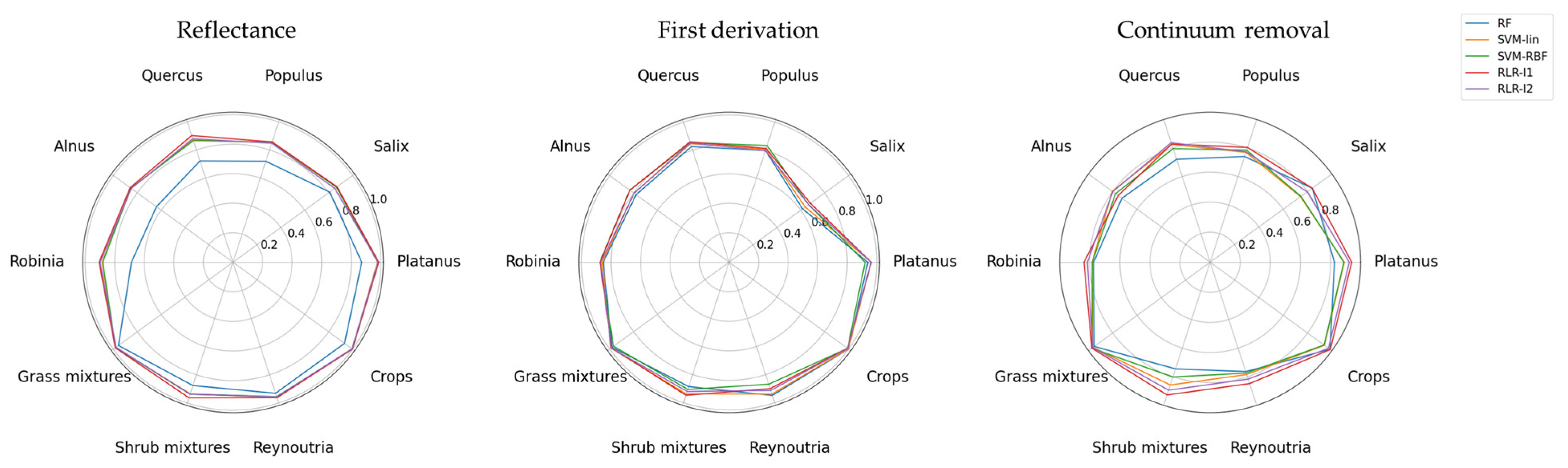
4.1.2. Performance Assessment

A high performance was obtained with all kinds of features. Indeed, AOA ranged from 83 to 94% across all scenarios (see Section 3.3.1). Without reducing the number of features, using original spectra led to better results than using continuum-removed or derivative spectra for all algorithms, except RF (

Table 6. Average Overall Accuracy (AOA) and standard deviation obtained from reflectance and transformations. The highest AOA is in bold and the lowest in italics.

Algorithm	Reflectance Spectra	First Derivative	Continuum Removal
RF	83 ± 2%	89 ± 1%	83 ± 3%
SVM—linear	93 ± 1%	90 ± 1%	86 ± 4%
SVM—RBF	93 ± 1%	89 ± 2%	85 ± 4%
RLR—ℓ1	94 ± 1%	91 ± 2%	90 ± 2%
RLR—ℓ2	93 ± 1%	90 ± 2%	88 ± 3%

). While transforming spectra caused a decrease of 3 to 8% AOA with SVM and RLR, transformations associated with RF led to an increase in AOA (+6% with derivation).

RLR with ℓ1 regularization provided the best results. Yet, used in conjunction with original spectra or first derivatives, the differences in AOA returned by the different algorithms were of the order of magnitude of the standard deviations. Only RF produced significantly lower results (2 to 11% lower). Figure 5 confirms this result. Overall, the classification maps have a very similar appearance.

Using continuum removal, RLR provided the highest AOA, followed by SVM and then RF. Since ℓ1 regularization embeds a feature selection, this result can underline a propensity to the Hughes phenomenon; it is more highly pronounced when using Random Forest. In the following paragraphs, RLR-ℓ1 was used as a basis for comparison since it provided the best results.

All feature reduction methods provided similar performances. Using 10 components was not sufficient to discriminate classes. Indeed, AOA was systematically lower using 10 components than more (Figure 6). Increasing the number of components from 10 to 20 led to an increase ranging from 2 to 5% with PCA, from 4 to 9% with MNF, from 3 to 7% with ICA, and from 4 to 6% with the SFFS. Subsequently, using more than 20 components did not provide significant progress (1 to 2%). Scores obtained with reflectance spectra were assessed with 20 features or more. Figure 6 highlights these results with RLR-ℓ1. All algorithms, including RF, provided similar results, highlighting the Hughes phenomenon for RF when used with too many features.

A similar trend was observed in the F1-scores. All classifiers struggled in discriminating tree genera, except for Platanus (e.g., using reflectance spectra, first derivation, and CR, Figure 7). F1-scores exceeded 0.93 for all classifiers (except RF) for grass mixtures, shrub mixtures, Reynoutria, crops, and Platanus discrimination. F1-scores ranged from 0.64 to 0.90 for the other classes. These difficulties were even more pronounced with RF: F1-scores ranged from 0.64 (Alnus) to 0.80 (Salix). Continuum removal provided significantly lower results regarding all classes and classifiers. The highest differences were observed for Reynoutria and shrub mixtures. Finally, using derivation, Salix pixels were poorly classified (F1-score of 0.61 to 0.68) with all classifiers.

Figure 8 compares classification maps obtained with RLR-ℓ1 (best AOA) and RF (worst AOA) applied to spectra. Differences in the predictions between the classifiers are presented in red. Tree genera classifications were consistent. The main differences were located in the borders of crowns.

The best classifier, RLR-ℓ1, was retained to illustrate the improvement of our rejection method (Figure 9). Even if pixels related to low represented species, unconsidered for the classification, were not predicted to the rejection class but in other tree species classes, the rejection class was found able to eliminate inconsistencies between the algorithms. Indeed, a part of mixed pixels located on the edges between different classes was rejected. Plus, the rejection class included pixels corresponding to unmasked non-pure vegetation pixels, such as the edges of roads (mixture of low vegetation and bare soil) or vegetation pixels mixed with electrical lines (framed in grey in Figure 9).

4.2. Multispectral Multitemporal Classification

4.2.1. Feature Selection by SFFS

Temporal Selection

Statistics and distances were computed from the time series to obtain the best date combinations (see Section 3.2.4). The seasonal selection led to the following dates: 26 January, 19 April, 18 July, and 22 November. The monthly selection provided: 26 January, 25 February, 10 March, 19 April, 26 May, 18 June, 18 July, 14 August, 23 September, 23 October, 22 November, 25 December.

SFFS-Based Temporal Selection

Applying SFFS in a spectral-temporal fashion (4 VNIR bands with 10m spatial resolution considered individually across the time series, see Section 3.2.2) led to 56 necessary features to separate all classes (one feature being one band at one specific date). Features selected more than once are analyzed in the following paragraphs.

In our context, from Sentinel-2 VNIR bands, green and red-edge bands were mandatory to separate the studied genera, especially during summer (June–September). Separating tree genera required the joint exploitation of several features, while the distinction of tree species from shrubs or grasses (shrubs mixtures, Reynoutria, and the grass mixtures) was made with one or two features.

The red-edge band predominated during the entire year to separate all kinds of genera, especially in summer (Figure 10). Five selections of this band appeared in July, including four on the 5th. Associated with other features, this feature allowed discriminating Alnus from Populus and Quercus, and grass mixtures from Reynoutria. Used alone, it allowed distinguishing Quercus from Reynoutria. Four selections were then obtained in August for the Platanus distinction, two at the beginning (on 2 August to distinguish it from Robinia and Reynoutria) and two others at the end of the month (on 22 August to separate it from grass and shrub mixtures). The red-edge band was then exploited seven times during spring, twice on 10 March for Alnus (distinction from Salix and Robinia), twice on 6 April for grass mixtures (distinction from Quercus and Alnus), twice on 26 May (Populus from Quercus and shrub mixtures from Reynoutria), and once on 19 April. Two selections were finally obtained on 13 October to separate Populus from Reynoutria and grass mixtures from shrub mixtures.

The green band was also of great interest for genera discrimination, especially in July. Indeed, this band was selected nine times on 5 July in conjunction with other features to discriminate Platanus from other broadleaf tree genera (Quercus, Alnus, and Robinia) as well as Salix from grass mixtures. Used alone, it allowed the discrimination between the tree genera and Reynoutria and shrubs (Populus, Quercus, and Robinia from shrub mixtures and Salix and Robinia from Reynoutria). A key date for the distinction of tree genera using the green band was the middle of September (the 13th). This date allowed distinguishing Salix from Platanus and Alnus.

Although secondary, the blue and red bands presented a non-negligible discriminatory power. The blue band was selected three times in spring (on 16 May) to separate Salix from Platanus, Populus, and grass mixtures, including two times in conjunction with the blue band in October (on 13 October for Salix, Platanus, and Populus). The distinction of Quercus from Populus and grass mixtures was obtained with this band on 20 November. Finally, the red band was used for Platanus’ separation from Alnus and shrub mixtures (on 18 June) and Alnus from Robinia and shrub mixtures from Reynoutria (on 10 November).

Adding indices covered by Sentinel-2 VNIR bands (10 m) in the SFFS selection, the importance of the green band on 7 May was again highlighted (selected five times; see Figure 11). This band was still prevalent since it was selected eight times (five times on 5 July, once on 16 May, 2 August, and 11 October). However, using indices plus bands rather than bands alone provided the importance of several indices rather than the red-edge band (Figure 11). Of all the features needed to separate all classes, the red-edge band was only directly selected once.

The predominant selected spectral feature was the green band followed by the red one, which was selected six times (on 4 April, 19 April, 18 June, 2 August, 22 August, and 20 November). Then, the GI index [52], which makes use of a ratio between the red and green bands, was returned five times throughout the year (on 29 January, 9 April, 26 May, 31 October, and 17 November). The same occurred for the Datt 2 index [52], which exploits the same bands but inverted (ratio between green and red bands). Next came the RVI, green NDVI, and MSR [52], which are all related to the red-edge band (four selections). Similarly, all indices returned three times, respectively, NDVI [52,71], OPTVI, and MTVI2, and four of the five indices returned twice to also make use of the red-edge [85]. Thus, the red-edge band was still found prevalent, but was more useful when used in conjunction with the other bands. This result was consistent with those explained above and was caused by the correlation between features. The blue band was again less useful than green and red-edge bands since it was directly selected only once (on 22 August) and retained in very few index formulations (twice in SIPI and NDVIGB [85], and once through EVI, NPCI, and CACOI [85]), and finally involved in 13% of selections. Regarding genera separation, only the green band on 5 July, Datt 2 on 19 April, and NDVI on 26 January were redundant, respectively, to distinguish shrubs from other genera/assemblages, and Platanus from other tree genera (Datt 2 and NDVI). Again, two to three features were used to distinguish tree genera, while only one could be exploited to separate shrubs (shrub mixtures and Reynoutria) from tree genera. This led to a total of 60 necessary features to separate all classes, while 56 features were used with spectral bands alone. Nevertheless, the exploitation of indices seemed to reduce the number of necessary features to separate 2 classes since less than 2 features were used to make 86% of the separations (11 separations with 1 and 20 with 2 features over 36 separations) against 50% with spectral bands alone (10 with 1 and 8 with 2 features over 36).

4.2.2. Performance Assessment

Moderate performance was obtained in all cases, ranging from 44% to 72% in terms of AOA with standard deviations ranging from 4 to 10%. The algorithms provided comparable results. However, RF seemed slightly outperformed since it provided the lowest AOA in 80% of scenarios (see Section 3.3.2). Conversely, the RLR-ℓ2 algorithm was particularly appropriate for multispectral multitemporal data since it was the best in 66% of scenarios. Nevertheless, RLR-ℓ1 was again used as a basis of comparison to illustrate similarities obtained with hyperspectral scenarios.

As observed with hyperspectral-based classifications, the best results were obtained using the most features or the most important ones. Indeed, increasing the number of exploited dates led to an increase in AOA (

Table 7. Average Overall Accuracy and corresponding standard deviations obtained with the different temporal selections. The highest AOA are in bold and the lowest in italics.

Algorithm	Seasonal 4 Dates	Monthly 12 Dates	All Dates 32 Dates	SFFS Selection 11 Dates
RF	56 ± 8%	59 ± 5%	61 ± 6%	60 ± 6%
SVM—linear	58 ± 8%	62 ± 6%	67 ± 6%	64 ± 5%
SVM—RBF	57 ± 9%	62 ± 4%	64 ± 6%	67 ± 5%
RLR—ℓ1	58 ± 5%	61 ± 6%	66 ± 6%	61 ± 6%
RLR—ℓ2	59 ± 5%	64 ± 4%	67 ± 5%	64 ± 4%

). Increasing from seasonal to monthly date selection led to an increase in the performance between 3 and 5%, while increasing it to the entire dataset rose AOA from 2 to 5% (reaching up to 67%). Using predominant dates, determined with SFFS (11 dates), scores ranged between 59 and 67%, highlighting that using well-chosen dates provided similar results as using all dates.

Regarding the spectral features, the exploitation of more spectral features increased the performance until a plateau was reached (around 65% AOA), as observed with hyperspectral imagery (Figure 12). Again, PCA, MNF, and ICA provided similar performances. With each feature extraction method, RF was outperformed by other algorithms, providing results 9 to 13% lower than others with a single component, 9 to 15% with 2, 7 to 8% with 3, and only 1 to 5% with 4 components. Thus, the gap between RF and other algorithms was reducing with the number of components. Using the features selected by SFFS, clear progress was visible from 1 to 10 features, as illustrated in Figure 12. In agreement with the SFFS selection, using bands plus indices rather than spectral bands alone slightly improved the results. With the RLR-ℓ2 algorithm, using eight features rather than the four bands increased AOA by 5%.

Tree genera were again the most difficult to classify whatever the number of exploited dates or features. For instance, SVM-linear using VNIR bands for all dates provided F1-scores ranging from 27% for Robinia to 72% for Platanus, while F1-scores for grass mixtures, shrub mixtures, and Reynoutria were all above 82%. The same went with scenarios providing high AOA, respectively, RLR-ℓ2 with all dates and bands (32 to 63% for tree genera in exception of Platanus, here at 80%) and SVM–RBF with SFFS selected dates. Looking at the best scenario, respectively, RLR-ℓ2 with all dates and eight features, the lowest F1-scores were also obtained for some tree genera, with the lowest scores for Robinia (44%), Alnus (53%), Salix (59%), and Quercus (63%). Yet, the scores were better for Populus (79%) than for Platanus, whose distinction was the easiest among the tree genera in most cases (76%), or even Reynoutria (72%).

Based on the differences in predictions between the different classification maps, located in red Figure 13, classifiers provided similar predictions on large, homogenous areas. They were, however, less reliable for heterogeneous areas or individuals, even with a tree crown close in the size of Sentinel-2 pixels, due to a priori mixed pixels. If the rejection class was again able to identify pixels corresponding to these differences with RLR, the chosen thresholds were too strict for RF or SVM and suppressed a major part of the classification maps (located in white in Figure 14). Indeed, the predicted probabilities were much larger (generally close to 1) with RLR than with other algorithms.

4.3. Spatial, Spectral, and Temporal Importance Assessment

As defined in Section 3.3.2 (Table 5), the hyperspectral image was degraded to the 10 m spatial resolution and the spectral domain was restricted to VNIR only. In addition, the spectral bands of Sentinel-2 were simulated from the hyperspectral image.

The most detailed spectral information at the finest spatial resolution (VNIR-SWIR at 1 m corresponding to the HS image, see

Table 8. Average Overall Accuracies (AOA) and corresponding standard deviations obtained with the different spectral and spatial configurations (MS: multispectral; HS: hyperspectral). The highest AOA is in bold and the lowest in italics.

	Sentinel-2 Time Series	Simulated Sentinel-2 VNIR Bands Derived from HS Image	Spatial Resampled HS Image		HS Image
Algorithm	MS VNIR (All Dates)	HS 4-Bands VNIR 1 m	HS VNIR 10 m	HS VNIR SWIR 10 m	HS VNIR 1 m	HS VNIR SWIR 1 m
RF	61 ± 6%	72 ± 2%	51 ±5%	50 ± 6%	80 ± 3%	83 ± 2%
SVM—linear	67 ± 6%	68 ± 3%	61 ± 8%	62 ± 6%	91 ± 1%	93 ± 1%
SVM—RBF	64 ± 4%	70 ± 3%	60 ± 6%	60 ± 4%	91 ± 1%	93 ± 1%
RLR—ℓ1	66 ± 6%	64 ± 3%	69 ± 5%	74 ± 4%	93 ± 1%	94 ± 1%
RLR—ℓ2	67 ± 5%	65 ± 2%	64 ± 10%	64 ± 11%	91 ± 2%	93 ± 1%

) provided the best performance in terms of AOA. At the same spatial resolution, discarding SWIR bands tended to slightly reduce performance (between 1 and 3% according to the classification algorithm considered). The simulation of Sentinel-2 spectral resolution bands at a 1 m spatial resolution provided a significant decline in performance (11 to 30%). These simulations proved the importance of spectral information for a 1 m spatial resolution in this context.

At a 10 m spatial resolution, the performance was similar for VNIR and VNIR-SWIR domains (deviation of 1%) with all algorithms except RLR-ℓ1. This result highlights the Hughes phenomenon caused by the low number of training samples for too many features. The importance of spatial resolution in our context, essential to increase the number of samples, was again demonstrated. In addition, restricting the spectral information to the VNIR only led to a reduction of a maximum of 5% of AOA (or to a reduction of 13 to 28% with Sentinel-2 bands) while keeping the entire spectrum, but reducing spatial information at 10 m caused a reduction of 21 to 34%.

When comparing temporal and spectral information using the same spectral domain (VNIR) and spatial resolution (10 m), the performance decreased by 3 to 10% with spectral richness, except with the RLR-ℓ1 classifier. The latter provided a performance increase of 3% due to its ability to select essential features. Thus, in our context, at a defined scale, spectral and temporal richness were comparable if well-processed. In addition, if no feature selection was made (all algorithms except RLR-ℓ1), temporal information was found to be slightly more appropriate.

Finally, in comparison with the use of the entire Sentinel-2 time series with a 10 m spatial resolution, RF and SVM (linear and RBF) provided higher AOA with the monodate Sentinel-2 1 m simulated image (+11, +6%, and +1%). The opposite was obtained with RLR classifiers (−2%). Again, this result highlights the propensity of the RLR classifier to handle the Hughes phenomenon since more features and fewer samples were involved in classifications using the entire time series than the simulated 1 m image. Regardless of the algorithms, a greater maximum AOA (+5%) was obtained using the 1 m simulated image. Spatial information was thus also found to be more important than temporal information in our context. The discrimination of tree genera was the main difficulty in all scenarios. Regarding the maps (Figure 15), the 10 m spatial resolution looked too coarse to identify isolated trees or to delimit genera in heterogeneous areas.

4.4. Biodiversity Assessment

Biodiversity metrics were derived from the best classification map (RLR-ℓ1 derived from HS reflectance spectra) both on the reference and impacted sites (

Table 9. Biodiversity metrics calculated from best classification maps on reference and impacted sites.

	Shannon	Simpson	Pielou Equitability	Simpson Equitability
Reference site	3.0	0.15	0.90	0.94
Impacted site	2.95	0.14	0.89	0.96

). No clear difference was observed between the two sites. The Shannon index, which could here range from 0 (homogeneous site) to 3.32 (heterogeneous distribution of species within the site), and the Pielou equitability (ratio of the Shannon index to its maximum) were close to their maxima with the 10 considered species, underlining the heterogeneity of the sites. The Simpson and equitability indices provided the same result, but slightly more drastically. Thus, the most common classes were slightly more homogeneously distributed than rare classes on both sites.

Crops were discarded at maximum for abundance analysis for two reasons: their presence on the hyperspectral-based classifications only and their unnatural presence. Regarding genera abundance over the impacted and the reference sites, fewer tree genera and Reynoutria numbers were observed on the impacted site, while grass and shrub mixtures were abundant (Figure 16). Grass mixtures’ predominance may be directly related to pipe burials or other numerous mechanical impacts occurring on the impacted area.

5. Discussion

5.1. Supervised Classification Methodology

5.1.1. Transformations and Feature Reduction

All feature extraction methods (PCA, MNF, ICA) led to similar classification performances. Hycza et al. systematically obtained better results using MNF than PCA on tree species classification with SVM [64]. The same results were obtained by Dabiri et al. using the RF algorithm, who found ICA to be even better than MNF [35]. These results can be explained by their choice of a number of components defined a priori. In our study, the number of components varied. Considering a specific classification algorithm, the ranking between feature extraction techniques changed with the number of components (Figure 6). Additionally, in these two studies, the number of components used with the different dimension reduction techniques was different. Hycza et al. used seven components with MNF and three with PCA, allowing more spectral information to be captured with MNF. Similarly, Dabiri et al. retained 20 components with PCA, 35 with MNF, and 27 with ICA. The choice of a fixed number of components, which differs according to the techniques, explains why one technique stood out in their case and not in ours.

If feature extraction methods provided better classification performances than feature selection methods (such as SFFS) in the literature [34,46], a similar performance was obtained in our case. However, as described by Dalponte et al., the ability of SFFS to highlight important spectral and temporal features makes it a useful tool for spectral analyses [37].

In our hyperspectral SFFS selection, green, red, red-edge, and SWIR domains were found to be the most important (see Section 4.1.1). This result is consistent with Hennessy’s meta-analysis on wavelength selection, which showed that these domains are involved in more than 50% of studies using the whole optical spectrum [54]. Then, if adding indices to hyperspectral bands did not improve our performance, this result is in line with Ferreira et al., Cui et al., and Erudel et al. [39,52,94]. Only Maschler et al. improved their classification by adding vegetation indices to reflectance values at specific hyperspectral bands. However, their images covered only the VNIR domain, thus dealing with fewer spectral features.

Our study reveals that the green and the red-edge spectral bands of Sentinel-2 VNIR bands are the most appropriate to discriminate our genera. This result is consistent with the literature. Hennessy et al. underlined that from studies using band selection on hyperspectral data, more than 70% of studies using VNIR only selected the bands between 550 and 600 nm [54]. If less than 40% of studies selected bands between 800 and 850 nm, the 10 m resolution Sentinel-2 red-edge band, centered at 832 nm, extends from around 780 to 885 nm and thus recovers several bands often selected, explaining the importance of this feature. In addition, the same study explained that this domain is particularly appropriate because of its link with chlorophyll [54]. Another interesting result provided by the SFFS is that combining indices based on red-edge with reflectance values at green and red bands seems more appropriate than using the red-edge band directly. This combination improved classification performance in our study (+5%). Other works obtained similar conclusions. Additionally, using a Sentinel-2 time series, Immitzer et al. increased their tree species classification (12 species) results by 5% by adding indices to spectral signatures, leading the way to an improvement similar to ours [95].

Regarding the time series analysis, most studies highlight the importance of spring and autumn to distinguish temperate shrub and tree species by underlining vegetation phenology [42,53,96]. Our results highlight the discriminatory power of summer dates, a result consistent with the visual analysis of the hyperspectral image acquired on 5 July, on which visible variations between genera are observable by photointerpretation. However, spring and autumn were still found essential, especially for tree genera distinction.

A possible way to improve performance could be the consideration of spectro-temporal features, defined from spectral values from several dates [45]. Grigorieva et al. thus defined new spectro-temporal features based on the correlation and differences between the spectral signatures from different phenophases. Such features allowed them to improve their tree species classification based on multispectral data (Landsat OLI) across two different sites.

5.1.2. Algorithm Comparison

A lot of studies define SVM or RF as state-of-the-art supervised classification algorithms for their efficiency and robustness [34,46,47]. In our context, the RLR algorithm provided a slightly better performance associated with multispectral images and greater performance with hyperspectral images at both 1 and 10 m spatial resolutions. The ability of RLR-ℓ1 seems particularly appropriate to prevent the Hughes phenomenon since this algorithm embeds a feature-selection step. A similar conclusion was obtained by Erudel et al. who compared these algorithms applied to in situ hyperspectral data to discriminate numerous peatland vegetation classes [52]. They exhibited classification performance improvement by applying transformations (in particular, the first and second order derivates) on spectral signatures. In our study, RF was more efficient when applied to the derivation or continuum removal of the spectral signature. Other algorithms provided their best results using reflectance spectra.

All algorithms were chosen among the most robust to the Hughes phenomenon [23,57]. However, the question of this effect appeared and resulted in a decreased performance for some algorithms, such as the RF algorithm. Feature reduction was found to be a necessary step in these specific cases, as observed by Dabiri et al. with RF for hyperspectral-based tree species classification and Burai et al. for alkali vegetation using both RF and SVM [35,41]. On the contrary, Dalponte et al. obtained lower results with SFFS selection than without considering RF [37]. Possible explanations lie in the difference between the considered features (spectral bands only in their case) and the low number of discriminated classes well represented. For their four-class problem (with two major classes), they used a similar number of pixels to our study. These classification conditions may have allowed them to avoid the Hughes phenomenon related to the RF classifier.

5.1.3. Rejection Method

The proposed rejection method allowed for improving classification maps and the consistency between classifiers by eliminating a part of pixels composed of many classes. However, the genera not considered for the classification for lack of referenced data (see Section 2.2), such as Fraxinus, Alnus, or Corylus, did not label to the rejection class with the considered rule due to the proximity between trees spectra (see Section 4.1.2 and Section 4.2.2). In addition, the application of this method on the time series of multispectral images only provided acceptable results when used in conjunction with the RLR algorithm. Further work on rejection class management should be conducted to predict this rejection class (the aim being that it identifies pixels belonging to a species or genera not represented in the training database). Possible ways to improve a posteriori rejection would be to consider the spatial context of each pixel or to define adaptative thresholds rather than empirical thresholds. For instance, Koerich et al. successfully defined different thresholding techniques for a handwritten word-recognition problem [97]. Otherwise, classification methods embedding rejection, such as the SegSALSA algorithm [65], should be compared to a posteriori rejection methods.

5.2. Classification Performance

5.2.1. Performance Comparison for Hyperspectral Image and Sentinel-2 Times Series

The hyperspectral-based global performance attained scores equivalent to those obtained for tree species classification problems (around 90%) [33,34,35,36,37,38,39]. A higher AOA was obtained from our complex site compare to other complex ecosystems (e.g., alkali landscape and aquatic vegetation) with hyperspectral-based classification at equivalent spatial resolutions [31,32].

The use of VNIR and SWIR jointly rather than VNIR alone only slightly improved the classification performance (less than 3% of differences in accuracy). This slight increase can be explained by the difference in spatial resolution (factor 2) between VNIR and SWIR (see Section 2.3.1). Similarly, Dalponte et al. also compared the use of VNIR alone and VNIR and SWIR jointly at different spatial resolutions (respectively 0.4 and 1.5 m) and found minor benefits for the use of SWIR for the classification of four tree species in a boreal forest [37]. Conversely, significant differences (up to a 14% increase in OA) were found in the Atlantic rainforest using a 1 m spatial resolution for both VNIR and SWIR [39].

The classification based on time series of multispectral images provided lower scores than the best of the state-of-the-art algorithms (maximum of 72% in AOA in our case). Indeed, several studies recently conducted on tree species returned results over 80% in OA [96,98,99]. Nonetheless, these studies were conducted in much larger areas, allowing the use of more samples within a class. For example, Grabska et al. classified 9 species in a mixed forest covering 240 km² (with 2433 reference pixels). Denisova et al. used 2000 pixels per class (9 tree species classes) selected in an area of 64.7 km² for training, and Bolyn et al. studied a forest of 3338.5 km² mostly composed of pure stands (11 tree species). It should still be noted that a similar performance was obtained for challenging shrub classification for a site wider than ours (1210 km²) using VNIR and SWIR Sentinel-2 bands [53]. In our context, the size and heterogeneity of the studied area (2.45 km², see Section 2.1) made the classification very challenging. At this scale, the lack of a sufficient number of pure pixels increased classification training and evaluation difficulties and led to results lower than those in state-of-the-art algorithms.

5.2.2. Comparison of Spectral, Spatial, and Temporal Information for Classification Improvement

In line with previous works, our approach confirmed that using multitemporal information improved genera/species discrimination in comparison to using a monodate image with the same spatial and spectral characteristics [42,53,96,100]. The temporal information compensated for the lack of spectral information in multispectral images for a given spatial resolution (10 m) in our classification context. Indeed, when degrading the spatial resolution of the hyperspectral image, both single-date hyperspectral and time series of multispectral images could achieve similar performances, as observed by Clark et al., Guidici et al., and Grigorieva et al. [43,44,45]. This proved the importance of phenology for vegetation-type discrimination. Kluczek et al. even proved that comparable performance could be achieved in homogeneous landscapes with different spatial resolutions [101]. Indeed, they achieved a similar performance with hyperspectral images at a 2 m spatial resolution and Sentinel-2 time series for the classification of 13 classes (rock scree communities, grassland, and forest type).

In our specific context, spatial resolution was mandatory. Significant differences occurred between the results provided by Sentinel-2 at a 10 m spatial resolution and hyperspectral data at a 1 m spatial resolution (+22%). Moreover, the degradation of the hyperspectral spatial resolution caused an important decrease when compared to the original hyperspectral image (−21 to −34%). A similar decrease (around −15%) was observed by Dalponte et al. when transitioning from a spatial resolution of 0.4 m to 1.5 m. Conversely, Ghosh et al. obtained equal performances at 4 m and 8 m spatial resolutions to classify five tree species. They explained their result by a lower intraspecific variance at 8 m than at 4 m. However, they kept the same number of samples at their different resolutions [50]. Roth et al. obtained their best results for genera/species classification with decametric spatial resolutions on five different sites (with herbaceous, shrubby, or woody vegetation added to soil and water classes according to the site) with significant differences in OA compared to metric resolutions (+1 to 18%). To obtain these results, they still had important databases, with up to 1940 samples at their coarser resolution (60 m). In addition, they had to discard up to five species (per site) that were under-represented at coarse resolutions. In our context, using a 10 m spatial resolution provided a significantly lower number of samples (183 pixels versus 24,670 pixels at a 1 m spatial resolution) without reducing the number of classes used. The strong heterogeneity of our sites could also affect our results since variance is not necessarily reduced by using a lower spatial resolution.

While the hyperspectral image was degraded to provide spectral characteristics (in terms of spectral resolution and domain) comparable to Sentinel-2 VNIR (see Section 3.3.2), the performance was far from the one obtained with the original hyperspectral VNIR SWIR image (−24% accuracy). When using a monodate image, a high number of spectral bands was thus necessary to distinguish genera in our context. Grigorieva et al. and Clark et al. obtained similar conclusions for forest classifications with a performance at least 10% higher with hyperspectral data than multispectral ones [45,102].

Airborne hyperspectral images are difficult to obtain and expensive. Evaluating the essential characteristics needed for various remote sensing applications, such as species classification or biodiversity assessment, is necessary to specify future hyperspectral satellite missions. Even if this study provided rich information for future satellite applications, our simulations were optimistic since realistic satellite characteristics (such as SNR—Signal-to-Noise Ratio and TMF—Transfer Modulation Function) were not considered for satellite image simulations. Recent and future satellite missions should allow hyperspectral acquisitions with a decametric spatial resolution and high temporal resolution [103,104,105,106,107]. PRISMA and EnMAP satellites are designed to reach a 30 m spatial resolution [105,106,107]. In our specific context, such a resolution does not provide a sufficient training database for classification at the genera level, but surely leads to a promising classification performance for less complex study sites (lower species number and more pixel numbers by class in the training database). The future hyperspectral satellite HYPXIM-Biodiversity mission with around a 10 m spatial resolution and 10 nm spectral resolution will be more suited to our study case [103,104]. In our context of high heterogeneity within a small surface area, such characteristics are mandatory to obtain a sufficient level of accuracy in vegetation mapping at the genera/species level.

Such existing or planned hyperspectral satellite missions could allow the accurate assessment and monitoring of biodiversity in the context of multiple anthropogenic impacts, including soil contamination.

5.3. Relation between Biodiversity and Anthropogenic Impacts

The quality of classification maps derived from hyperspectral or multispectral images at the genus level is good, even in a difficult context with multiple anthropogenic impacts similar to our study site.

The high spatial heterogeneity in species representation may have highlighted the limitations of Sentinel-2, even if the most homogeneous areas were mapped similarly with both instruments. Nevertheless, only the hyperspectral data could be used for the biodiversity assessment since the classification maps varied significantly between iterations or algorithms for the Sentinel-2 data. Differences in relative genera abundance were found between the reference and the impacted sites. However, they may be due to differences in maintenance (e.g., cutting frequencies and passages of vehicles) or development of the environment (e.g., exposure and slope), rather than the influence of soil properties. Both Reynoutria and Rubus (main component of shrub mixtures), are known to be widespread species resistant to severe soil contamination [108,109]. Therefore, the presence of shrub mixtures rather than Reynoutria in the impacted site is not necessarily indicative of anthropogenic soil impacts. Biodiversity metrics were consistent between the sites. However, they were calculated per pixel, regardless of the size of units or minority species. Oniya et al. found significant differences in biodiversity indices values based on the spectral variation hypothesis created on Sentinel-2 images [18]. Such an approach allows rare species to be considered. Although effective, they require multiple field surveys that are possibly difficult in certain contexts [110]. In addition, Gholizadeh et al. proved the necessity to consider soil properties [111]. With appropriate field data, it could be interesting to compare biodiversity metrics derived from species mapping and the spectral variation hypothesis. In our context, local analyses of correlation between species, their spectra, and local impacts should be investigated in future works.

6. Conclusions

This study aimed to first evaluate the performance of supervised classification techniques for complex vegetation classification in the context of anthropogenic impacts. To assess the potential of state-of-the-art methods, multi-modal imagery was exploited: single-date metric hyperspectral images at a metric spatial resolution and time series of multispectral images with a decametric spatial resolution. Ten genera and assemblages, including tree, shrub, and herbaceous species, were mapped in an area of 2.45 km². While hyperspectral-based classification allowed raising the performance up to 94%, using the multispectral Sentinel-2 time series only permitted reaching 72% of the Average Overall Accuracy. In both cases, the six deciduous tree genera were the principal cause of confusion. The weak performance of the time series of multispectral images was explained by its decametric spatial resolution and its spectral resolution. The heterogeneity in vegetation units, species, and especially in spatial arrangement explained the difficulty to obtain a better performance.

From the considered spectral transformations, only indices applied to the time series of multispectral images improved the performance. With the hyperspectral image, the best results were obtained directly from reflectance spectra. No feature reduction was found better than others in this study. All allowed us to avoid the Hughes phenomenon. The performance obtained using the reflectance spectra was retrieved with a lower number of features. The use of selected features by SFFS provided similar performance results, but allowed identifying the discriminating characteristics of each species. While the RLR algorithm is used less frequently than SVM or RF in the published works, it provided a better performance in our complex context. The propensity of the ℓ1 regularization to embed feature selection makes this algorithm particularly suitable for high-dimensional data, such as hyperspectral images. The ℓ2 regularization, which avoids redundancy between features, is also interesting for multitemporal classifications. Yet, since all algorithms provided similar performances, combining the maps provided by the various classifiers could improve classification performances and lead to a more robust merged map [112].

Few studies in the literature address an exhaustive comparison of the spectral, spatial, and temporal contributions for classification purposes. In our study, spatial information was found to be predominant. At a defined scale, spectral and temporal richness were comparable. In the future, similar simulations will be performed by introducing the future HYPXIM-Biodiversity hyperspectral satellite mission specifications (spectral/spatial resolutions, spectral sampling, TMF, SNR).

The proposed rejection method showed promising results to deal with the high species spatial repartition variability and minor species in the context of anthropogenic impacts. If this method showed its limitation as the thresholds must be adapted to the study case and processed data, mixed pixels often fall in the rejection class. Using adaptative thresholds could provide a more robust method [97]. Rejection methods using contextual spatial information should additionally be considered to both limit the salt and pepper effect and better detect minority species [65].

Deriving biodiversity metrics from the resulting vegetation maps did not provide significant differences between the impacted and reference sites. Nevertheless, vegetation mapping showed inconsistencies in genera distribution potentially related to anthropogenic impacts. A lower proportion of tree genera and Reynoutria was found on the impacted site than on the reference one, while grass and shrub mixtures were more abundant. Biodiversity assessments based on the spectral variability hypothesis and field data survey should be considered to verify these conclusions.

This work will continue with a more precise analysis of the spatial distribution of the various impacts and species. At the species level, species sensitive to the different impacts will be identified. Their spectral signatures and biophysicochemical parameters will be analyzed in both the reference and impacted sites to determine the impacted traits. Finally, the same study will be conducted on another impacted site to consolidate the results.

References

1. Ong, C.; Carrère, V.; Chabrillat, S.; Clark, R.; Hoefen, T.; Kokaly, R.; Marion, R.; Souza Filho, C.R.; Swayze, G.; Thompson, D.R. Imaging Spectroscopy for the Detection, Assessment and Monitoring of Natural and Anthropogenic Hazards. Surv. Geophys. 2019, 40, 431–470. [Google Scholar] [CrossRef] [Green Version]
2. Cunningham, C.; Beazley, K.F. Changes in human population density and protected areas in terrestrial global biodiversity hotspots, 1995–2015. Land 2018, 7, 136. [Google Scholar] [CrossRef] [Green Version]
3. Dietz, T.; Rosa, E.A.; York, R. Driving the human ecological footprint. Front. Ecol. Environ. 2007, 5, 13–18. [Google Scholar] [CrossRef]
4. Lassalle, G. Monitoring natural and anthropogenic plant stressors by hyperspectral remote sensing: Recommendations and guidelines based on a meta-review. Sci. Total Environ. 2021, 788, 147758. [Google Scholar] [CrossRef] [PubMed]
5. Holloway, J.; Mengersen, K. Statistical machine learning methods and remote sensing for sustainable development goals: A review. Remote Sens. 2018, 10, 1365. [Google Scholar] [CrossRef] [Green Version]
6. Gholizadeh, A.; Kopačková, V. Detecting vegetation stress as a soil contamination proxy a review of optical proximal and remote sensing techniques. Int. J. Environ. Sci. Technol. 2019, 16, 2511–2524. [Google Scholar] [CrossRef]
7. Miller, V.S.; Naeth, M.A. Hydrogel and Organic Amendments to Increase Water Retention in Anthroposols for Land Reclamation. Appl. Environ. Soil Sci. 2019, 2019, 4768091. [Google Scholar] [CrossRef]
8. Obour, P.B.; Ugarte, C.M. A meta-analysis of the impact of traffic-induced compaction on soil physical properties and grain yield. Soil Tillage Res. 2021, 211, 105019. [Google Scholar] [CrossRef]
9. Lwin, C.S.; Seo, B.H.; Kim, H.U.; Owens, G.; Kim, K.R. Application of soil amendments to contaminated soils for heavy metal immobilization and improved soil quality—A critical review. Soil Sci. Plant Nutr. 2018, 64, 156–167. [Google Scholar] [CrossRef]
10. Lassalle, G.; Fabre, S.; Credoz, A.; Hédacq, R.; Bertoni, G.; Dubucq, D.; Elger, A. Application of PROSPECT for estimating total petroleum hydrocarbons in contaminated soils from leaf optical properties. J. Hazard. Mater. 2019, 377, 409–417. [Google Scholar] [CrossRef] [Green Version]
11. Ignat, T.; De Falco, N.; Berger-Tal, R.; Rachmilevitch, S.; Karnieli, A. A novel approach for long-term spectral monitoring of desert shrubs affected by an oil spill. Environ. Pollut. 2021, 289, 117788. [Google Scholar] [CrossRef]
12. Pérez-Hernández, I.; Ochoa-Gaona, S.; Adams, R.H.; Rivera-Cruz, M.C.; Pérez-Hernández, V.; Jarquín-Sánchez, A.; Geissen, V.; Martínez-Zurimendi, P. Growth of four tropical tree species in petroleum-contaminated soil and effects of crude oil contamination. Environ. Sci. Pollut. Res. 2017, 24, 1769–1783. [Google Scholar] [CrossRef]
13. Matsodoum Nguemté, P.; Djumyom Wafo, G.V.; Djocgoue, P.F.; Kengne Noumsi, I.M.; Wanko Ngnien, A. Potentialities of Six Plant Species on Phytoremediation Attempts of Fuel Oil-Contaminated Soils. Water. Air. Soil Pollut. 2018, 229, 88. [Google Scholar] [CrossRef]
14. Pérez-Hernández, I.; Ochoa-Gaona, S.; Adams Schroeder, R.H.; Rivera-Cruz, M.C.; Geissen, V. Tolerance of four tropical tree species to heavy petroleum contamination. Water. Air. Soil Pollut. 2013, 224, 1637. [Google Scholar] [CrossRef]
15. Rola, K.; Osyczka, P.; Nobis, M.; Drozd, P. How do soil factors determine vegetation structure and species richness in post-smelting dumps? Ecol. Eng. 2015, 75, 332–342. [Google Scholar] [CrossRef]
16. Válega, M.; Lillebø, A.I.; Pereira, M.E.; Duarte, A.C.; Pardal, M.A. Long-term effects of mercury in a salt marsh: Hysteresis in the distribution of vegetation following recovery from contamination. Chemosphere 2008, 71, 765–772. [Google Scholar] [CrossRef] [Green Version]
17. Anawar, H.M.; Canha, N.; Santa-Regina, I.; Freitas, M.C. Adaptation, tolerance, and evolution of plant species in a pyrite mine in response to contamination level and properties of mine tailings: Sustainable rehabilitation. J. Soils Sediments 2013, 13, 730–741. [Google Scholar] [CrossRef]
18. Onyia, N.N.; Balzter, H.; Berrio, J.C. Spectral diversity metrics for detecting oil pollution effect on biodiversity in the niger delta. Remote Sens. 2019, 11, 2662. [Google Scholar] [CrossRef] [Green Version]
19. Clark, M.L.; Roberts, D.A.; Clark, D.B. Hyperspectral discrimination of tropical rain forest tree species at leaf to crown scales. Remote Sens. Environ. 2005, 96, 375–398. [Google Scholar] [CrossRef]
20. Ustin, S.L.; Gitelson, A.A.; Jacquemoud, S.; Schaepman, M.; Asner, G.P.; Gamon, J.A.; Zarco-Tejada, P. Retrieval of foliar information about plant pigment systems from high resolution spectroscopy. Remote Sens. Environ. 2009, 113, S67–S77. [Google Scholar] [CrossRef] [Green Version]
21. Misra, G.; Cawkwell, F.; Wingler, A. Status of phenological research using sentinel-2 data: A review. Remote Sens. 2020, 12, 2760. [Google Scholar] [CrossRef]
22. Transon, J.; d’Andrimont, R.; Maugnard, A.; Defourny, P. Survey of hyperspectral Earth Observation applications from space in the Sentinel-2 context. Remote Sens. 2018, 10, 157. [Google Scholar] [CrossRef] [Green Version]
23. Ghamisi, P.; Plaza, J.; Chen, Y.; Li, J.; Plaza, A.J. Advanced Spectral Classifiers for Hyperspectral Images: A review. IEEE Geosci. Remote Sens. Mag. 2017, 5, 8–32. [Google Scholar] [CrossRef] [Green Version]
24. Zhang, Z.; Liu, M.; Liu, X.; Zhou, G. A new vegetation index based on multitemporal sentinel-2 images for discriminating heavy metal stress levels in rice. Sensors 2018, 18, 2172. [Google Scholar] [CrossRef] [Green Version]
25. Lassalle, G.; Elger, A.; Credoz, A.; H’dacq, R.; Bertoni, G.; Dubucq, D.; Fabre, S. Toward quantifying oil contamination in vegetated areas using very high spatial and spectral resolution imagery. Remote Sens. 2019, 11, 2241. [Google Scholar] [CrossRef] [Green Version]
26. Adamu, B.; Tansey, K.; Bradshaw, M.J. Investigating vegetation spectral reflectance for detecting hydrocarbon pipeline leaks from multispectral data. Image Signal Process. Remote Sens. XIX 2013, 8892, 889216. [Google Scholar] [CrossRef]
27. Onyia, N.N.; Balzter, H.; Berrio, J.C. Detecting vegetation response to oil pollution using hyperspectral indices. In Proceedings of the IGARSS 2018–2018 IEEE International Geoscience and Remote Sensing Symposium, Valencia, Spain, 22–27 July 2018; pp. 3963–3966. [Google Scholar] [CrossRef]
28. Asri, N.A.M.; Sakidin, H.; Othman, M.; Matori, A.N.; Ahmad, A. Analysis of the hydrocarbon seepage detection in oil palm vegetation stress using unmanned aerial vehicle (UAV) multispectral data. AIP Conf. Proc. 2020, 2266, 050007. [Google Scholar] [CrossRef]
29. Cochrane, M.A. Using vegetation reflectance variability for species level classification of hyperspectral data. Int. J. Remote Sens. 2000, 21, 2075–2087. [Google Scholar] [CrossRef]
30. Skidmore, A.K.; Coops, N.C.; Neinavaz, E.; Ali, A.; Schaepman, M.E.; Paganini, M.; Kissling, W.D.; Vihervaara, P.; Darvishzadeh, R.; Feilhauer, H.; et al. Priority list of biodiversity metrics to observe from space. Nat. Ecol. Evol. 2021, 5, 896–906. [Google Scholar] [CrossRef] [PubMed]
31. Rocchini, D.; Hernández-Stefanoni, J.L.; He, K.S. Advancing species diversity estimate by remotely sensed proxies: A conceptual review. Ecol. Inform. 2015, 25, 22–28. [Google Scholar] [CrossRef]
32. Fassnacht, F.E.; Müllerová, J.; Conti, L.; Malavasi, M.; Schmidtlein, S. About the link between biodiversity and spectral variation. Appl. Veg. Sci. 2022, 25, e12643. [Google Scholar] [CrossRef]
33. Dian, Y.; Li, Z.; Pang, Y. Spectral and Texture Features Combined for Forest Tree species Classification with Airborne Hyperspectral Imagery. J. Indian Soc. Remote Sens. 2015, 43, 101–107. [Google Scholar] [CrossRef]
34. Fassnacht, F.E.; Neumann, C.; Forster, M.; Buddenbaum, H.; Ghosh, A.; Clasen, A.; Joshi, P.K.; Koch, B. Comparison of feature reduction algorithms for classifying tree species with hyperspectral data on three central european test sites. IEEE J. Sel. Top. Appl. Earth Obs. Remote Sens. 2014, 7, 2547–2561. [Google Scholar] [CrossRef]
35. Dabiri, Z.; Lang, S. Comparison of independent component analysis, principal component analysis, and minimum noise fraction transformation for tree species classification using APEX hyperspectral imagery. ISPRS Int. J. Geo-Inf. 2018, 7, 488. [Google Scholar] [CrossRef] [Green Version]
36. Raczko, E.; Zagajewski, B. Comparison of support vector machine, random forest and neural network classifiers for tree species classification on airborne hyperspectral APEX images. Eur. J. Remote Sens. 2017, 50, 144–154. [Google Scholar] [CrossRef] [Green Version]
37. Dalponte, M.; Ørka, H.O.; Gobakken, T.; Gianelle, D.; Næsset, E. Tree species classification in boreal forests with hyperspectral data. IEEE Trans. Geosci. Remote Sens. 2013, 51, 2632–2645. [Google Scholar] [CrossRef]
38. Ballanti, L.; Blesius, L.; Hines, E.; Kruse, B. Tree species classification using hyperspectral imagery: A comparison of two classifiers. Remote Sens. 2016, 8, 445. [Google Scholar] [CrossRef] [Green Version]
39. Ferreira, M.P.; Zortea, M.; Zanotta, D.C.; Shimabukuro, Y.E.; de Souza Filho, C.R. Mapping tree species in tropical seasonal semi-deciduous forests with hyperspectral and multispectral data. Remote Sens. Environ. 2016, 179, 66–78. [Google Scholar] [CrossRef]
40. Burai, P.; Deák, B.; Valkó, O.; Tomor, T. Classification of herbaceous vegetation using airborne hyperspectral imagery. Remote Sens. 2015, 7, 2046–2066. [Google Scholar] [CrossRef] [Green Version]
41. Burai, P.; Lövei, G.; Lénárt, C.; Nagy, I.; Enyedi, E. Mapping aquatic vegetation of the Rakamaz-Tiszanagyfalui Nagy-Morotva using hyperspectral imagery. Landsc. Environ. 2010, 4, 1–10. [Google Scholar]
42. Hill, R.A.; Wilson, A.K.; George, M.; Hinsley, S.A. Mapping tree species in temperate deciduous woodland using time-series multi-spectral data. Appl. Veg. Sci. 2010, 13, 86–99. [Google Scholar] [CrossRef]
43. Guidici, D.; Clark, M.L. One-dimensional convolutional neural network land-cover classification of multi-seasonal hyperspectral imagery in the San Francisco Bay Area, California. Remote Sens. 2017, 9, 629. [Google Scholar] [CrossRef] [Green Version]
44. Clark, M.L.; Buck-Diaz, J.; Evens, J. Mapping of forest alliances with simulated multi-seasonal hyperspectral satellite imagery. Remote Sens. Environ. 2018, 210, 490–507. [Google Scholar] [CrossRef]
45. Grigorieva, O.; Brovkina, O.; Saidov, A. An original method for tree species classification using multitemporal multispectral and hyperspectral satellite data. Silva Fenn. 2020, 54, 1–17. [Google Scholar] [CrossRef] [Green Version]
46. Fassnacht, F.E.; Latifi, H.; Stereńczak, K.; Modzelewska, A.; Lefsky, M.; Waser, L.T.; Straub, C.; Ghosh, A. Review of studies on tree species classification from remotely sensed data. Remote Sens. Environ. 2016, 186, 64–87. [Google Scholar] [CrossRef]
47. Gewali, U.B.; Monteiro, S.T.; Saber, E. Machine learning based hyperspectral image analysis: A survey. arXiv 2018, arXiv:1802.08701v2. [Google Scholar]
48. Lu, D.; Weng, Q. A survey of image classification methods and techniques for improving classification performance. Int. J. Remote Sens. 2007, 28, 823–870. [Google Scholar] [CrossRef]
49. Zhang, J.; Rivard, B.; Sánchez-Azofeifa, A.; Castro-Esau, K. Intra- and inter-class spectral variability of tropical tree species at La Selva, Costa Rica: Implications for species identification using HYDICE imagery. Remote Sens. Environ. 2006, 105, 129–141. [Google Scholar] [CrossRef]
50. Ghosh, A.; Fassnacht, F.E.; Joshi, P.K.; Kochb, B. A framework for mapping tree species combining hyperspectral and LiDAR data: Role of selected classifiers and sensor across three spatial scales. Int. J. Appl. Earth Obs. Geoinf. 2014, 26, 49–63. [Google Scholar] [CrossRef]
51. Lim, J.; Kim, K.M.; Jin, R. Tree species classification using hyperion and sentinel-2 data with machine learning in South Korea and China. ISPRS Int. J. Geo-Inf. 2019, 8, 150. [Google Scholar] [CrossRef] [Green Version]
52. Erudel, T.; Fabre, S.; Houet, T.; Mazier, F.; Briottet, X. Criteria Comparison for Classifying Peatland Vegetation Types Using In Situ Hyperspectral Measurements. Remote Sens. 2017, 9, 748. [Google Scholar] [CrossRef] [Green Version]
53. Macintyre, P.; van Niekerk, A.; Mucina, L. Efficacy of multi-season Sentinel-2 imagery for compositional vegetation classification. Int. J. Appl. Earth Obs. Geoinf. 2020, 85, 101980. [Google Scholar] [CrossRef]
54. Hennessy, A.; Clarke, K.; Lewis, M. Hyperspectral Classification of Plants: A Review of Waveband Selection Generalisability. Remote Sens. 2020, 12, 113. [Google Scholar] [CrossRef] [Green Version]
55. Ghiyamat, A.; Shafri, H.Z.M.; Mahdiraji, G.A.; Shariff, A.R.M.; Mansor, S. Hyperspectral discrimination of tree species with different classifications using single- and multiple-endmember. Int. J. Appl. Earth Obs. Geoinf. 2013, 23, 177–191. [Google Scholar] [CrossRef]
56. Hughes, G.F. On the Mean Accuracy of Statistical Pattern Recognizers. IEEE Trans. Inf. Theory 1968, 14, 55–63. [Google Scholar] [CrossRef] [Green Version]
57. Pal, M.; Foody, G.M. Feature selection for classification of hyperspectral data by SVM. IEEE Trans. Geosci. Remote Sens. 2010, 48, 2297–2307. [Google Scholar] [CrossRef] [Green Version]
58. Hameed, S.S.; Petinrin, O.O.; Hashi, A.O.; Saeed, F. Filter-wrapper combination and embedded feature selection for gene expression data. Int. J. Adv. Soft Comput. Its Appl. 2018, 10, 90–105. [Google Scholar]
59. Dumont, J.; Hirvonen, T.; Heikkinen, V.; Mistretta, M.; Granlund, L.; Himanen, K.; Fauch, L.; Porali, I.; Hiltunen, J.; Keski-Saari, S.; et al. Thermal and hyperspectral imaging for Norway spruce (Picea abies) seeds screening. Comput. Electron. Agric. 2015, 116, 118–124. [Google Scholar] [CrossRef]
60. Pant, P.; Heikkinen, V.; Korpela, I.; Hauta-Kasari, M.; Tokola, T. Logistic regression-based spectral band selection for tree species classification: Effects of spatial scale and balance in training samples. IEEE Geosci. Remote Sens. Lett. 2014, 11, 1604–1608. [Google Scholar] [CrossRef]
61. Gimenez, R.; Lassalle, G.; Hédacq, R.; Elger, A.; Dubucq, D.; Credoz, A.; Jennet, C.; Fabre, S. Exploitation of Spectral and Temporal Information for Mapping Plant Species in a Former Industrial Site. Int. Arch. Photogramm. Remote Sens. Spat. Inf. Sci. 2021, XLIII-B3-2, 559–566. [Google Scholar] [CrossRef]
62. Torabzadeh, H.; Leiterer, R.; Hueni, A.; Schaepman, M.E.; Morsdorf, F. Tree species classification in a temperate mixed forest using a combination of imaging spectroscopy and airborne laser scanning. Agric. For. Meteorol. 2019, 279, 107744. [Google Scholar] [CrossRef]
63. Zhang, C.; Xie, Z. Object-based vegetation mapping in the kissimmee river watershed using hymap data and machine learning techniques. Wetlands 2013, 33, 233–244. [Google Scholar] [CrossRef]
64. Hycza, T.; Stereńczak, K.; Bałazy, R. Potential use of hyperspectral data to classify forest tree species. N. Z. J. For. Sci. 2018, 48, 18. [Google Scholar] [CrossRef]
65. Condessa, F.; Bioucas-Dias, J.; Kovacevic, J. Supervised hyperspectral image classification with rejection. In Proceedings of the 2015 IEEE International Geoscience and Remote Sensing Symposium (IGARSS), Milan, Italy, 26–31 July 2015; pp. 2600–2603. [Google Scholar] [CrossRef]
66. Aval, J. Automatic Mapping of Urban Tree Species Based on Multi-Source Remotely Sensed Data. Ph.D. Thesis, Université de Toulouse, Toulouse, France, 2018. [Google Scholar]
67. Lassalle, G.; Fabre, S.; Credoz, A.; Hédacq, R.; Dubucq, D.; Elger, A. Mapping leaf metal content over industrial brownfields using airborne hyperspectral imaging and optimized vegetation indices. Sci. Rep. 2021, 11, 2. [Google Scholar] [CrossRef]
68. BD ORTHO® IGN Website. Available online: https://geoservices.ign.fr/bdortho (accessed on 2 February 2022).
69. Brigot, G.; Colin-Koeniguer, E.; Plyer, A.; Janez, F. Adaptation and Evaluation of an Optical Flow Method Applied to Coregistration of Forest Remote Sensing Images. IEEE J. Sel. Top. Appl. Earth Obs. Remote Sens. 2016, 9, 2923–2939. [Google Scholar] [CrossRef] [Green Version]
70. Theia. Produits à Valeur Ajoutée et al. Gorithmes pour les Surfaces Continentales. Available online: https://www.theia-land.fr/ (accessed on 13 January 2022).
71. Fabre, S.; Gimenez, R.; Elger, A.; Rivière, T. Unsupervised Monitoring Vegetation after the Closure of an ore Processing Site with Multi-temporal Optical Remote Sensing. Sensors 2020, 20, 4800. [Google Scholar] [CrossRef]
72. Waqar, M.M.; Mirza, J.F.; Mumtaz, R.; Hussain, E. Development of new indices for extraction of built-up area & bare soil from landsat data. Open Access Sci. Rep. 2012, 1, 4. [Google Scholar]
73. Valdiviezo-N, J.C.; Téllez-Quiñones, A.; Salazar-Garibay, A.; López-Caloca, A.A. Built-up index methods and their applications for urban extraction from Sentinel 2A satellite data: Discussion. JOSA A 2018, 35, 35–44. [Google Scholar] [CrossRef]
74. Du, Y.; Zhang, Y.; Ling, F.; Wang, Q.; Li, W.; Li, X. Water bodies’ mapping from Sentinel-2 imagery with Modified Normalized Difference Water Index at 10-m spatial resolution produced by sharpening the swir band. Remote Sens. 2016, 8, 354. [Google Scholar] [CrossRef] [Green Version]
75. Rasul, A.; Balzter, H.; Ibrahim, G.R.F.; Hameed, H.M.; Wheeler, J.; Adamu, B.; Ibrahim, S.; Najmaddin, P.M. Applying built-up and bare-soil indices from Landsat 8 to cities in dry climates. Land 2018, 7, 81. [Google Scholar] [CrossRef] [Green Version]
76. Huete, A.R. A soil-adjusted vegetation index (SAVI). Remote Sens. Environ. 1988, 25, 295–309. [Google Scholar] [CrossRef]
77. Pearson, R.L.; Miller, L.D. Remote mapping of standing crop biomass for estimation of the productivity of the shortgrass prairie. In Proceedings of the Eighth International Symposium on Remote Sensing of Environment, Ann Arbor, MI, USA, 2–6 October 1972; Willow Run Laboratories, Environmental Research Institute of Michigan: Ann Arbor, MI, USA, 1972; p. 1355. [Google Scholar]
78. Nagao, M.; Matsuyama, T.; Ikeda, Y. Region extraction and shape analysis in aerial photographs. Comput. Graph. Image Process. 1979, 10, 195–223. [Google Scholar] [CrossRef]
79. Smith, P.; Reid, D.B.; Environment, C.; Palo, L.; Alto, P.; Smith, P.L. NOBUYUKI OTSU.-1979-A Tlreshold Selection Method from Gray-Level Histograms. IEEE Trans. Syst. Man Cybern. 1979, 20, 62–66. [Google Scholar]
80. Vluymans, S. Learning from imbalanced data. Stud. Comput. Intell. 2019, 807, 81–110. [Google Scholar] [CrossRef]
81. Baldeck, C.A.; Asner, G.P. Improving remote species identification through efficient training data collection. Remote Sens. 2014, 6, 2682–2698. [Google Scholar] [CrossRef] [Green Version]
82. Karasiak, N.; Dejoux, J.F.; Monteil, C.; Sheeren, D. Spatial dependence between training and test sets: Another pitfall of classification accuracy assessment in remote sensing. Mach. Learn. 2022, 111, 2715–2740. [Google Scholar] [CrossRef]
83. Karasiak, N.; Dejoux, J.F.; Fauvel, M.; Willm, J.; Monteil, C.; Sheeren, D. Statistical stability and spatial instability in mapping forest tree species by comparing 9 years of satellite image time series. Remote Sens. 2019, 11, 2512. [Google Scholar] [CrossRef] [Green Version]
84. Xue, J.; Su, B. Significant remote sensing vegetation indices: A review of developments and applications. J. Sens. 2017, 2017, 1353691. [Google Scholar] [CrossRef] [Green Version]
85. Erudel, T. Caractérisation de la Biodiversité Végétale et des Impacts Anthropiques en Milieu Montagneux par Télédétection: Apport des Données Aéroportées à Très haute Résolution Spatiale et Spectrale. Ph.D. Thesis, Onera-Geode Labex DRIIHM, Toulouse, France, 2018. [Google Scholar]
86. Pedregosa, F.; Varoquaux, G.; Gramfort, A.; Michel, V.; Thirion, B.; Grisel, O.; Blondel, M.; Prettenhofer, P.; Weiss, R.; Dubourg, V.; et al. Scikit-learn: Machine Learning in Python. J. Mach. Learn. Res. 2012, 12, 2825–2830. [Google Scholar]
87. Breiman, L. Random forests. Mach. Learn. 2001, 45, 5–32. [Google Scholar] [CrossRef] [Green Version]
88. Vapnik, V. Statistical Learning Theory; Wiley: New York, NY, USA, 1998; Volume 1, p. 2. [Google Scholar]
89. Stehman, S.V.; Czaplewski, R.L. Design and Analysis for Thematic Map Accuracy Assessment—An application of satellite imagery. Remote Sens. Environ. 1998, 64, 331–344. [Google Scholar] [CrossRef]
90. Peet, R.K. The measurement of species diversity. Annu. Rev. Ecol. Syst. 1974, 5, 285–307. [Google Scholar] [CrossRef]
91. Fedor, P.; Zvaríková, M. Biodiversity indices. Encycl. Ecol. 2019, 2, 337–346. [Google Scholar]
92. Wang, R.; Gamon, J.A.; Cavender-Bares, J.; Townsend, P.A.; Zygielbaum, A.I. The spatial sensitivity of the spectral diversity-biodiversity relationship: An experimental test in a prairie grassland. Ecol. Appl. 2018, 28, 541–556. [Google Scholar] [CrossRef] [Green Version]
93. Sun, Y.; Huang, J.; Ao, Z.; Lao, D.; Xin, Q. Deep learning approaches for the mapping of tree species diversity in a tropical wetland using airborne LiDAR and high-spatial-resolution remote sensing images. Forests 2019, 10, 1047. [Google Scholar] [CrossRef] [Green Version]
94. Cui, L.; Zuo, X.; Dou, Z.; Huang, Y.; Zhao, X.; Zhai, X.; Lei, Y.; Li, J.; Pan, X.; Li, W. Plant identification of Beijing Hanshiqiao wetland based on hyperspectral data. Spectrosc. Lett. 2021, 54, 381–394. [Google Scholar] [CrossRef]
95. Immitzer, M.; Neuwirth, M.; Böck, S.; Brenner, H.; Vuolo, F.; Atzberger, C. Optimal input features for tree species classification in Central Europe based on multi-temporal Sentinel-2 data. Remote Sens. 2019, 11, 2599. [Google Scholar] [CrossRef] [Green Version]
96. Grabska, E.; Hostert, P.; Pflugmacher, D.; Ostapowicz, K. Forest stand species mapping using the sentinel-2 time series. Remote Sens. 2019, 11, 1197. [Google Scholar] [CrossRef] [Green Version]
97. Koerich, A.L. Rejection strategies for handwritten word recognition. In Proceedings of the Ninth International Workshop on Frontiers in Handwriting Recognition, Kokubunji, Japan, 26–29 October 2004; pp. 479–484. [Google Scholar] [CrossRef] [Green Version]
98. Denisova, A.; Kavelenova, L.; Korchikov, E.; Prokhorova, N.; Terentyeva, D.; Fedoseev, V. Tree species classification for clarification of forest inventory data using Sentinel-2 images. In Proceedings of the Seventh International Conference on Remote Sensing and Geoinformation of the Environment (RSCy2019), Paphos, Cyprus, 18–21 March 2019; Volume 1117408, p. 3. [Google Scholar] [CrossRef]
99. Bolyn, C.; Michez, A.; Gaucher, P.; Lejeune, P.; Bonnet, S. Forest mapping and species composition using supervised per pixel classification of Sentinel-2 imagery. Biotechnol. Agron. Soc. Environ. 2018, 22, 16. [Google Scholar] [CrossRef]
100. Persson, M.; Lindberg, E.; Reese, H. Tree species classification with multi-temporal Sentinel-2 data. Remote Sens. 2018, 10, 1794. [Google Scholar] [CrossRef] [Green Version]
101. Kluczek, M.; Zagajewski, B.; Kycko, M. Airborne HySpex Hyperspectral Versus Multitemporal Sentinel-2 Images for Mountain Plant Communities Mapping. Remote Sens. 2022, 14, 1209. [Google Scholar] [CrossRef]
102. Clark, M.L. Comparison of multi-seasonal Landsat 8, Sentinel-2 and hyperspectral images for mapping forest alliances in Northern California. ISPRS J. Photogramm. Remote Sens. 2020, 159, 26–40. [Google Scholar] [CrossRef]
103. Briottet, X.; Asner, G.P.; Bajjouk, T.; Carrère, V.; Chabrillat, S.; Chami, M.; Chanussot, J.; Dekker, A.; Delacourt, C.; Feret, J.-B. European hyperspectral explorer: Hypex-2. Monitoring anthropogenic influences in critical zones. In Proceedings of the 10. EARSeL SIG Imaging Spectroscopy Workshop, Zurich, Switzerland, 19–21 April 2017. 11p. [Google Scholar]
104. Briottet, X.; Marion, R.; Carrere, V.; Jacquemoud, S.; Chevrel, S.; Prastault, P.; D’oria, M.; Gilouppe, P.; Hosford, S.; Lubac, B. HYPXIM: A new hyperspectral sensor combining science/defence applications. In Proceedings of the 2011 3rd Workshop on Hyperspectral Image and Signal Processing: Evolution in Remote Sensing (WHISPERS), Lisbon, Portugal, 6–9 June 2011; pp. 1–4. [Google Scholar]
105. Galeazzi, C.; Sacchetti, A.; Cisbani, A.; Babini, G. The PRISMA program. In Proceedings of the IGARSS 2008-2008 IEEE International Geoscience and Remote Sensing Symposium, Boston, MA, USA, 7–11 July 2008; Volume 4, pp. IV-105–IV-108. [Google Scholar]
106. Stuffler, T.; Kaufmann, C.; Hofer, S.; Förster, K.P.; Schreier, G.; Mueller, A.; Eckardt, A.; Bach, H.; Penné, B.; Benz, U. The EnMAP hyperspectral imager—An advanced optical payload for future applications in Earth observation programmes. Acta Astronaut. 2007, 61, 115–120. [Google Scholar] [CrossRef]
107. Lee, C.M.; Cable, M.L.; Hook, S.J.; Green, R.O.; Ustin, S.L.; Mandl, D.J.; Middleton, E.M. An introduction to the NASA Hyperspectral InfraRed Imager (HyspIRI) mission and preparatory activities. Remote Sens. Environ. 2015, 167, 6–19. [Google Scholar] [CrossRef]
108. Ibrahimpašić, J.; Jogić, V.; Toromanović, M.; Džaferović, A.; Makić, H.; Dedić, S. Japanese Knotweed (Reynoutria japonica) as a Phytoremediator of Heavy Metals. J. Agric. Food Environ. Sci. 2020, 74, 45–53. [Google Scholar] [CrossRef]
109. Steingräber, L.F.; Ludolphy, C.; Metz, J.; Germershausen, L.; Kierdorf, H.; Kierdorf, U. Heavy metal concentrations in floodplain soils of the Innerste River and in leaves of wild blackberries (Rubus fruticosus L. agg.) growing within and outside the floodplain: The legacy of historical mining activities in the Harz Mountains (Germany). Environ. Sci. Pollut. Res. 2022, 29, 22469–22482. [Google Scholar] [CrossRef]
110. Rocchini, D.; Balkenhol, N.; Carter, G.A.; Foody, G.M.; Gillespie, T.W.; He, K.S.; Kark, S.; Levin, N.; Lucas, K.; Luoto, M.; et al. Remotely sensed spectral heterogeneity as a proxy of species diversity: Recent advances and open challenges. Ecol. Inform. 2010, 5, 318–329. [Google Scholar] [CrossRef]
111. Gholizadeh, H.; Gamon, J.A.; Zygielbaum, A.I.; Wang, R.; Schweiger, A.K.; Cavender-Bares, J. Remote sensing of biodiversity: Soil correction and data dimension reduction methods improve assessment of α-diversity (species richness) in prairie ecosystems. Remote Sens. Environ. 2018, 206, 240–253. [Google Scholar] [CrossRef]
112. Knauer, U.; von Rekowski, C.S.; Stecklina, M.; Krokotsch, T.; Minh, T.P.; Hauffe, V.; Kilias, D.; Ehrhardt, I.; Sagischewski, H.; Chmara, S.; et al. Tree species classification based on hybrid ensembles of a convolutional neural network (CNN) and random forest classifiers. Remote Sens. 2019, 11, 2788. [Google Scholar] [CrossRef] [Green Version]
Figure 1. Study site’s location on a high-resolution orthophoto background (BD ORTHO® 20 cm [68]): Industrial brownfield (surrounded in red) and reference site (surrounded in blue).
Remotesensing 14 03633 g001
Figure 2. Dates of the Sentinel-2 time series acquired in 2017 (date format: MM/DD).
Remotesensing 14 03633 g002
Figure 3. General classification method flowchart.
Remotesensing 14 03633 g003
Figure 4. Feature selection frequency by the SFFS.
Remotesensing 14 03633 g004
Figure 5. Classification maps obtained with (a) RF, (b) SVM-linear, (c) SVM-RBF, (d) RLR-ℓ1, and (e) RLR-ℓ2.
Remotesensing 14 03633 g005
Figure 6. Average Overall Accuracy (AOA, in %; ± standard deviations) variations according to the selected component number with the RLR-ℓ1 algorithm for the three reduction techniques (PCA, MNF, and ICA).
Remotesensing 14 03633 g006
Figure 7. Average F1-scores obtained with reflectance spectra, first derivation, and continuum removal.
Remotesensing 14 03633 g007
Figure 8. Subset of class prediction differences between RLR-ℓ1 classification map and RF map.
Remotesensing 14 03633 g008
Figure 9. Subset of RLR-ℓ1 map with rejection class (in white). Electrical lines are framed in gray.
Remotesensing 14 03633 g009
Figure 10. Temporal selection obtained with SFFS for each VNIR spectral band.
Remotesensing 14 03633 g010
Figure 11. Band and index frequencies returned by temporal SFFS.
Remotesensing 14 03633 g011
Figure 12. Average Overall Accuracy (±standard deviations) returned by the different algorithms according to the number of selected features.
Remotesensing 14 03633 g012
Figure 13. Prediction differences (in red) between RLR-ℓ1 classification map and RF map.
Remotesensing 14 03633 g013
Figure 14. Illustration of the rejection class (in white) with (a) RLR-ℓ1 and (b) RF classification maps.
Remotesensing 14 03633 g014
Figure 15. Subset of RLR-ℓ1 classification map without the rejection class obtained with (a) MS VNIR, (b) HS VNIR 10 m, and (c) HS VNIR 1 m.
Remotesensing 14 03633 g015
Figure 16. Relative genera abundance as determined by RLR-ℓ1 hyperspectral classification in Materials and Methods Section.
Remotesensing 14 03633 g016