Hyperbola Detection with RetinaNet and Comparison of Hyperbola Fitting Methods in GPR Data from an Archaeological Site

Abstract

Hyperbolic diffractions in Ground Penetrating Radar (GPR) data are caused by a variety of subsurface objects such as pipes, stones, or archaeological artifacts. Supplementary to their location, the propagation velocity of electromagnetic waves in the subsurface can be derived. In recent years, it was shown that deep learning tools can automatically detect hyperbola in radargrams using data measured over urban infrastructure, which are relatively clear. In contrast, in this study, we used an archaeological dataset with diverse underground structures. In the first step we used the deep learning network RetinaNet to detect hyperbola automatically and achieved an average precision of 0.58. In the next step, 10 different approaches for hyperbola fitting and thus velocity determination were applied. The derived information was validated with manually determined velocities and apex points. It was shown that hyperbola extraction by using a threshold and a column connection clustering (C3) algorithm followed by simple hyperbola fitting is the best method, which had a mean velocity error of 0.021 m/ns compared to manual determination. The average 1D velocity-depth distribution derived in 10 ns intervals was in shape comparable to the manually determined one, but had a systematic shift of about 0.01 m/ns towards higher velocities.

1. Introduction

Hyperbolic diffractions in Ground Penetrating Radar (GPR) data are caused by a variety of subsurface objects such as pipes, cables, stones, or archaeological artifacts. The spatial distribution of their apex points can aid to investigate the spatial distribution of these subsurface structures. Additional information derivable from the hyperbola is the propagation velocity of electromagnetic waves in the subsurface, which is needed to determine the depth of the objects and/or the 3D-distribution of the water content of the soil.

With the advent of multi-channel GPR antenna arrays, it has become easy to cover large areas in short time with high spatial sampling, i.e., inline and crossline trace distances of 4 and 8 cm, respectively [1]. This leads to large data volumes, from which often only a small portion of information is taken out for interpretation. On the one hand, for some applications this is sufficient, e.g., for delineating structures in timeslices such as pipes or rebar. On the other hand, this limited output of information is also due to high costs and time in experienced manpower to inspect the data carefully in all aspects. However, the latter can be supported by machine learning algorithms that became widely used in the last decades and have also been used in the context of GPR processing to automatically detect pipes or rebar [2,3,4,5,6,7,8], defects in concrete [9], tree roots [10,11,12], and in radargrams or archaic hearths in timeslices [13].

Most articles on hyperbola detection use a two-step approach or focus just on one of the steps. The first step is to detect the hyperbola in the radargram (spatial coordinate and traveltime) and the second step is to derive information such as the velocity or radius of the pipe from its shape. Whereas this procedure is easily applied to the detection of, e.g., pipes in urban environments, where radargrams are often relatively clear and simple, examples with applications to archaeology in a rather natural environment are missing. This might be because a straight line of hyperbola detected on parallel profiles is easy to connect to a pipe, but archaeological objects causing diffractions are not necessarily in line. In addition, pipes in urban environments are located in a relatively homogeneous background, whereas the subsurface of archaeological sites can be very heterogeneous and thus show complicated radargrams.

The automatic detection of hyperbolas in radargrams can be accomplished with artificial neural networks, where the radargram is seen as an image. Object detection in images is widely conducted using machine learning and deep learning [14]. Often used networks in the context of object detection in images are R-CNN (regions with convolutional neural network) [15], Faster R-CNN [16], Cascade R-CNN [17], SSD (Single shot multibox detector) [18], YOLO (You Only Look Once) [19,20], or RetinaNet [21,22] to name just a few. The architecture of these networks can be built in deep learning frameworks such as pytorch, keras, or Matlab’s Deep Learning toolbox. To avoid the large number of images required for training, they can also be used as pretrained models in transfer learning to be adapted to the specific problem, which in our case is the detection of hyperbola in radargrams.

Probably the first paper using a simple artificial neural network in order to detect hyperbolas in radargrams was by the authors of ref. [2]. They fed a binary image of the radargram into a neural network with two layers and received the apex points of the hyperbola. Since about the year 2010, the number of articles using neural networks for apex detection has increased. Ref. [23] used a neural network of four layers with trapezoidal shaped images of hyperbola as training images. Unfortunately, no specific evaluation of the number of well- and misclassified hyperbola was provided. Since the advent of convolutional neural network (CNN) for object detection and classification in images [14], some of the above mentioned common deep convolutional networks have also been applied to radargrams and the detection of hyperbola, e.g., refs. [6,8,9,24,25].

One group of these networks is called region-based convolutional neural networks (R-CNN) [15] and has gained increased speed over time (Fast and Faster R-CNN [16,26]). Faster R-CNN uses a CNN first in order to generate feature maps of the input image. Then, a region proposal network (RPN) is applied on the feature maps, which is again a CNN with some more layers, in order to propose regions in the image that are likely to contain objects. In a last step, the proposed regions are fed into another neural network with fully connected layers in order to extract bounding box coordinates and a classification of the object. The bounding box coordinates are the pixel-based coordinates of a box around the object in the original image. Faster R-CNN has been used for hyperbola detection by, e.g., refs. [6,8,24].

A different network design has the YOLO (You Only Look Once) [19,20] object detector and its enhancements (up to YOLOv5). It also uses a deep CNN, but the input image is split into an S × S grid and for each of the grid cells a classification and bounding box regression is determined, which are combined in the end into final detections. This one-stage procedure has the advantage of being faster than the two-stage R-CNN detectors mentioned above. YOLOv5 was used by ref. [9] for detecting internal defects in asphalt from GPR data.

Once a hyperbola is detected, its shape can be used to determine the propagation velocity of electromagnetic waves. The mostly mentioned method to derive the velocity from the shape of the hyperbola is the Hough transform [27,28,29,30,31,32,33], which is a computationally intensive gridsearch. Another approach is the fitting of detected points on the hyperbolic signature with orthogonal distance fitting [34] or the Random Sample Consensus (RANSAC) [35].

In all the articles mentioned above, the comparison between automatically determined hyperbola parameters (which are in a reasonable range) and the ones manually derived by an experienced operator are missing. So how correct is the automatic determination, and what do these hyperbola parameters tell us? Obviously, the horizontal apex location provides the horizontal location of the scattering object, e.g., the pipe, rebar, root, or stone. The derived propagation velocity can be used to calculate the depth of the object from the traveltime to the apex. In case studies dealing with the urban detection of pipes or rebar, this is sufficient to delineate the underground infrastructure. However, what if the hyperbola originates from single stones or objects spread across an archaeological site? Conducting a multichannel GPR survey with small profile spacing across a single stone will result in diffraction hyperbola on several neighboring channels, i.e., the diffraction pattern is a hyperboloid in 3D. They will reveal the same velocity, but obviously have different apex locations on the neighboring radargrams, although they originate from one object. In addition, the subsurface on archaeological sites is mostly very heterogeneous compared with concrete bridge decks or asphalt in urban environments. Thus, we can expect heterogeneous radargrams with overlapping structures that mask the hyperbola.

So the questions that arise are:

• How effective and accurate is the use of an artificial neural network (RetinaNet in our case) in order to automatically detect hyperbola on large scale multi-channel GPR data measured on an archaeological site?
• Which fitting method for velocity determination is best and how accurate is the velocity determination compared to manual interpretation?

To answer these questions, we used a Malå MIRA (Mala Imaging Radar) GPR dataset collected using 16 channels measured on the archaeological site of Goting on the island of Föhr in Northern Germany. This site yields a stratified settlement with occupation phases ranging from the Younger Roman Iron Age to the High Medieval Period. In the area selected for measurements, prior magnetic survey and archaeological excavations have revealed divided areas used for residential and artisanal, harbor-related activities during the Early Medieval Period (8th–11th century AD), including cultural layers, workshop spaces, sunken-feature buildings, wells, and numerous ditches, forming parcellations and yard divisions [36,37,38]. The radargrams show a variety of archaeological features such as pits and dipping layers, but also a lot of diffraction hyperbola. The data quality in most of the 1.7 ha area was good and penetration depth reached 3–4 m. In the first step, we used this data to train a RetinaNet for automatic detection of hyperbola. RetinaNet has not been used for hyperbola detection before, but has shown to outperform other CNNs in object detection [21] and thus is promising for detecting hyperbola in radargrams. In the next step, the velocity and apex location were determined using different methods that are basically edge extraction and subsequent template matching and hyperbola fitting approaches. They are explained in detail below. The quality of detection and velocity determination for each method is be investigated on a smaller part of the area.

2. Materials and Methods

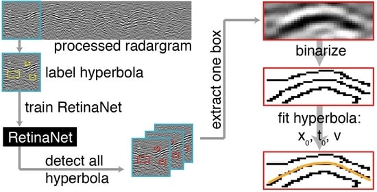
In this section, we first focus on the GPR data acquisition and processing and then provide an overview on RetinaNet, which was used to detect the hyperbola in the radargrams. Afterwards we show the further evaluation of the detected hyperbola, i.e., velocity derivation by different methods and clustering. A general overview of data preparation and the further procedure is also shown in the schematic in Figure 1 and explained in detail in the following parts.

2.1. GPR Data Acquisition and Processing

The GPR dataset was recorded with a Malå Multichannel Imaging Radar (MIRA) with 16 channels and 400 MHz center frequency. The time range of 100 ns was recorded at 1024 samples and the signal was stacked 4 times. Profile spacing was 8 cm and inline trace distance 3 cm. Accurate positioning was achieved with a Leica total station (TS15).

The data processing was performed with the MATLAB software MultichannelGPR [39] and consists of (a) DC amplitude removal, (b) time zero correction by shifting of channels 2–15 with relation to channel 1 for each profile by means of cross correlation, (c) adjustment of time zero across all profiles for all channels, (d) bandpass filtering (100–600 MHz), (e) cutting of the time axis at 80 ns, (f) application of a custom gain function with [−20, 0, 10, 20, 30 dB] stretched over the time range of 80 ns, and (g) removal of horizontal reflections with the help of a wavenumber highpass with cutoff wavenumber 0.1 m⁻¹.

The processed radargrams of all 16 channels were exported as jpeg images using a color scale with the highest 1% of amplitudes as black and the lowest 1% of amplitudes as white and gray scale in between. They were cut into pictures of 256 × 256 pixel size, i.e., 256 traces and the time range of 80 ns was spread onto 256 pixels, while recording the coordinates of each picture in a look-up table for later use. The gray-scale pictures were exported as RGB (red-green-blue) images and thus have three color values for each pixel, as was required for input into the pre-trained RetinaNet.

All 636 images of channel 1 containing hyperbola were used for training and evaluation of the Deep Learning network RetinaNet. The jpeg images of this channel were loaded into MATLAB Image Labeler and bounding boxes were manually assigned to the hyperbola. Then the data was split into 60% training data (381 images), 30% test data (191 images), and 10% validation data (64 images). In these 636 images, 1158 hyperbola were marked manually by bounding boxes as ground truth.

2.2. Hyperbola Detection with RetinaNet

Hyperbola in radargrams can be seen analogous to objects in images. For the detection and classification of objects in images, a wide range of tools exists. All these object detectors have to be trained on labeled images. This means that bounding boxes with a classification (called ground truth) have to be drawn manually in a number of images used for training. During training, a so-called loss function is minimized, which is roughly said to be the summed differences between the ground truth and detected box coordinates (bounding box regression) and the summed differences between the ground truth and detected classes (classification). When training is completed, the current weights of the network layers are fixed and new images can be fed into the network for object detection.

In this study, we used RetinaNet [21,22], which is based on Faster R-CNN [16] combined with a Feature Pyramid Network (FPN). A FPN takes the input image and applies convolutional layers to derive feature maps at different levels. This combination allows the extraction of both low-resolution, semantically strong features and high-resolution, semantically weak features. In addition, to overcome the problem of class imbalance between few objects and a large number of background samples, a new loss function is used, which is called focal loss [21]. For more details on the network see the references above.

We did not build the network from scratch, but used an existing RetinaNet in a pytorch implementation [40]. Its architecture is described in Appendix A. For classification, two classes were used: background and hyperbola, which is not a pre-existing class, but was defined by us. We used ResNet50 (Residual Network with 50 layers) [41] as the backbone with pretrained weights on the Microsoft COCO dataset [42] to reduce the training duration. This enables the network to extract features for detecting objects, but not explicitly hyperbola. In order to train the network further to detect the new object class “hyperbola”, we used our training dataset (381 images from channel 1, see above) as input. During this training we used an Adam optimizer with a learning rate of 1 × 10⁻⁵ and reduced the learning rate by multiplication with 0.1 if the loss remained constant over three epochs. One epoch is over if all images used for training are passed through the network. In total, 50 epochs were used. Different batch sizes (1, 2, 4, 8, 16) were tested. This batch size provides the number of images after which the weights of the network layers are adjusted. The calculations were performed on a high-performance computing cluster on 32 Intel Xeon x86-64 cores. The images of the validation dataset were used for performance evaluation during training and the test dataset for the final evaluation after training was completed. The models for different batch sizes were evaluated by calculating the average precision (AP), recall, and precision from the test data. Recall provides the number of actually detected hyperbola (Recall = TP/(TP + FN) with TP: true positive, FN: false negative) and the precision answers the question of how many of the detected hyperbola are actually hyperbola (Precision = TP/(TP + FP) with FP: false positive) [43]. These two measures were calculated for the first input image and subsequently updated after each following input image and could thus be plotted as a recall–precision curve. The area under the recall–precision curve is called average precision (AP).

After training was completed, all images from all other GPR channels were used as input for the trained RetinaNet and bounding boxes for classified hyperbola were inferred.

2.3. Velocity Derivation from Detected Hyperbola

While the accuracy of the hyperbola detection can be evaluated with the labeled test dataset (AP, recall, precision), we would also like to investigate the accuracy of apex and velocity derivation from the detected hyperbola. Therefore, a smaller test area of 10 m × 15 m was cut from the large dataset. The detected hyperbola in this area were then evaluated with different methods in order to derive the apex location (x₀ and t₀) and the velocity of the overlying medium. The results of the different methods, which are explained in the following subsections, are evaluated with respect to runtime and accuracy. For the accuracy determination, we derived the “true” apex location and velocity for each of the detected hyperbola manually by means of visually fitting a hyperbola to the radargram. In order to determine the error of apex and velocity determination during manual picking, we carried out this determination three times and calculated the mean and standard deviation. The test velocities were defined from 0.05 up to 0.15 m/ns in steps of 0.005 m/ns. This range was also used as a “valid data range” for the velocities during automatic determination.

The “true” apex locations and velocities, i.e., defined by mean and standard deviation from the three picking passes, were compared to the automatically derived ones by means of RMS errors (Root Mean Square errors). For all the automatic methods, the images in the smaller area were loaded and the detected bounding boxes were extracted. The following procedure applied to the bounding boxes could then be divided into two steps: (1) extraction of potential points on a hyperbola and (2) fitting of these points. For the extraction of potential points on a hyperbola, we used three methods, i.e., a Canny edge filter, minimum and maximum phase, and a threshold combined with subsequent column connection clustering (C3) algorithm. For fitting and deriving the hyperbola parameters, we used template matching (only applied to Canny edge-filtered images), Random Sample Consensus (RANSAC), Hough transform (HT), and least-squares fitting of x²-t²-pairs (Figure 2).

All of these methods have been used individually in the literature before, but we wanted to compare all combinations on a single dataset. This resulted in, overall, 10 different methods for automatic velocity determination inside the bounding boxes: (1) Template matching, (2) Canny edge and RANSAC, (3) Canny edge and HT, (4) Canny edge and x²-t²-fitting, (5) Min/max phase and RANSAC, (6) Min/max phase and HT, (7) Min/max phase and x²-t²-fitting, (8) Threshold and C3 and RANSAC, (9) Threshold and C3 and HT, and (10) Threshold and C3 and x²-t²-fitting. The different parts of these methods are explained in the following sections. To receive valid parameters during hyperbola fitting, we applied following restrictions to the derived parameters or otherwise set them to “invalid”: (a) the velocity has to be between 0.05 and 0.15 m/ns, and (b) the apex location (x₀ and t₀) has to be inside the bounding box.

2.3.1. Canny Edge Filter

Ref. [44] proposed a filter to detect edges in noisy images. They first applied a Gaussian filter to suppress noise and then calculated the intensity gradient of the smoothed gray-scale image. Afterwards, the pixels with gradients above a certain threshold were marked as strong edges and between this upper and a second lower threshold as weak edges. All pixels with gradients below the lower threshold were suppressed. In our applied MATLAB function for Canny edge detection, the upper threshold was selected automatically depending on the input data and the lower threshold was determined as 0.4 times the upper threshold. The resulting image was a binary image where 1 represents an edge and 0 the background.

2.3.2. Minimum and Maximum Phase

A very simple hyperbola point extraction method was inspired by ref. [45], who took the minimum phase points of each trace of a detected hyperbola. Therefore, we took the minimum and maximum amplitude point of each trace, resulting in two sets of points for fitting: one from the minima and one from the maxima. Unfortunately, they do not necessarily need to originate from the detected hyperbola, but could also stem from other high amplitude reflections in the current bounding box. After fitting each set individually, the determined parameters x₀, t₀, and v were averaged. Of course the apex times of minimum and maximum phase were different, but nevertheless, the mean value provides a robust estimate of the temporal location.

2.3.3. Threshold and Column Connection Clustering (C3) Algorithm

This method was proposed by ref. [33] and includes first the selection of regions of interest by thresholding the radargram and later thinning the regions of interest by finding connected clusters on neighboring traces. We selected half of the maximum amplitude in each detected bounding box as threshold and set all pixels with absolute amplitude above this threshold to one and below to zero. Then the resulting binary image was scanned column-wise from left to right in order to separate different regions into connected clusters. In a column a number of consecutive points higher than s (s = 3 in our case) is called a column segment. If there is a point in the same row on a neighboring column, it is called a connecting element. For each column segment in the first column, it is checked for a connecting element in the second column. If there is a connecting element in the second column with column segment length ≥ s, the cluster will continue. It is also possible that clusters split into two or more clusters. A detailed description of the algorithm can be found in ref. [33]. For each output cluster of the C3 algorithm, a central string is determined, which is composed of the middle points of the elements in each column for one cluster. Because there are probably more clusters in a bounding box, we chose the one with the longest central string, i.e., the highest number of connected columns and disregarded all other clusters. The points of the longest central string were then used for further fitting.

Because the small images as input for the hyperbola detection are relatively coarse with respect to temporal time step dt = 0.31 ns, using the cut-outs of bounding boxes from these input images resulted in no connecting elements. In order to achieve better correspondence between neighboring traces, i.e., more connecting elements, we upsampled the images inside the bounding boxes to dt/4 by linear interpolation before thresholding and C3 application.

2.3.4. Template Matching

Template matching for hyperbola detection was already applied by ref. [46] using modeled radargrams as templates. In contrast to using radargrams as input and test image, we used binary representations for both. First, a Canny edge filter was applied to the extracted bounding boxes resulting in binary images and then these binary images were compared with hyperbola templates using a 2D normalized cross correlation. The hyperbola templates were created for different apex times (t₀ between 0 and 79 ns in steps of the sample interval dt) and propagation velocities (v between 0.05 and 0.15 m/ns in steps of 0.005 m/ns). The resulting cross correlation maps for each velocity were searched for maximum values. To prevent the search to be trapped into local minima at the border, the cross correlation values were weighted with the inverse distance to the zero lag point. Thus, correlations near the center (minimum lags in x and t direction) were amplified. This assumption is valid because the bounding boxes were mostly located with the hyperbola in the middle in x direction and at the top in t direction, which is in accordance with the templates and thus close to zero lag. The location of the global maximum value of the weighted maps then indicates the best velocity and apex location.

2.3.5. Random Sample Consensus (RANSAC)

The RANSAC (Random Sample Consensus) algorithm [34] can be used to fit a model to noisy data by detecting and ignoring outliers. In our case the model is the equation for a hyperbola:

$$t_i=2\sqrt{{\left(\frac{t_0}{2}\right)}^2+{\left(\frac{x_i-x_0}{v}\right)}^2}$$

(1)

with t_i: two-way-traveltime at location x_i, t₀: two-way-traveltime at apex location x₀, and v: propagation velocity. Our noisy data consists of m x-t-pairs derived from the methods explained in Section 2.3.1, Section 2.3.2, Section 2.3.3 and for a well-determined set of equations we need at least three of these m points for fitting and deriving the three unknown parameters x₀, t₀, and v. For the RANSAC algorithm, we defined a number of sample points n (in our case n = 3) that were randomly taken from the m input points. Subsequently the model was fitted to these randomly chosen sample points and the number of points from the complete dataset within a certain error tolerance e (in our case e = 5 pixels in time direction) is determined. We call these points inliers as opposed to outliers. This was performed 50 times (in our case) and the sampling subset with the maximum number of inliers used to fit the model and derive the unknown parameters finally. For this final fitting, not only the n subset points were used, but rather the n points plus i inliers.

2.3.6. Hough Transform (HT)

The Hough transform (HT) was originally intended for finding straight lines in an image [47], but was further extended for the detection of general geometrical shapes in binary images [48]. A hyperbola can also be such a geometrical shape, which is described by the three parameters x₀, t₀, and v. All points derived by the methods explained in Section 2.3.1, Section 2.3.2, Section 2.3.3 were transformed into the parameter or Hough space according to the equation for a hyperbola (Equation (1)). The Hough space was determined by the valid ranges of the three unknown parameters: v between 0.05 and 0.15 m/ns, t₀ in the time range of the bounding box and x₀ around the vertical symmetry axis ±w/4, where w is the width of the bounding box. The location of the vertical symmetry axis was determined by calculating the symmetry of the binary image inside the bounding box as provided by ref. [29] and references therein. As maximum calculation column width, we used w again. This reduction of the valid parameter range of x₀ decreased the calculation time of the HT.

For all points taken from the binary image, the temporal apex location t₀ was calculated for all x₀ and v combinations using Equation (1). If the calculated t₀ was within the valid range, the Hough space at this location (x₀, t₀, v) increased by one. The point with the maximum number of counts was taken as the best match.

2.3.7. Least-Squares Fitting of x² − t²-Pairs

By rearranging Equation (1) one can yield

$${\left(\frac{t}{2}\right)}^2={\left(\frac{t_0}{2}\right)}^2+{\left(\frac{1}{v}\right)}^2{\left(x-x_0\right)}^2$$

(2)

which corresponds to a linear equation of type y′ = a + mx′ with $y^{\prime }={\left(\frac{t}{2}\right)}^2$, $a={\left(\frac{t_0}{2}\right)}^2$, $m={\left(\frac{1}{v}\right)}^2$ and $x^{\prime }={\left(x-x_0\right)}^2$. Thus, the velocity v can be directly derived from the slope and t₀ from the intercept of a straight line fitting pairs of x′ and y′. The apex location x₀ is determined by fitting a straight line to x′-t′-pairs with all different x′ taken as x₀. The fit with the smallest RMS error indicates the right x₀ value.

2.4. Clustering of Hyperbola

In rebar or pipe detection, it is relatively straightforward to connect detected apex points of hyperbola arranged in a straight line to one object, e.g., a pipe. In an archaeological context, where hyperbolae originate mainly from point-like objects such as stones, these will produce hyperbola on adjacent profiles all originating from a single point. Therefore, one has to find these hyperbolae belonging together and determine the true location of the object.

In order to group hyperbolae originating from the same subsurface object, we applied Density-Based Spatial Clustering of Applications with Noise (DBSCAN) [49]. The input data for the algorithm are the 3D locations of the determined apex points provided by Easting, Northing, and z. The depth z is determined by z = t₀/2 × v. The velocity v for this calculation is not taken from the automatic determination directly, but from a linear fit of the mean velocities determined in time intervals of 10 ns starting from 0 ns reaching to 80 ns. If the automatically determined velocities would have been taken, errors in them would result in very different depths of the hyperbola belonging to one cluster and thus they would not be clustered. When a mean velocity is taken instead, outliers are neglected and clustering is more robust.

For clustering, first, one point of this input data was chosen as current point and all points within a certain radius r (0.25 m in our case) were defined as neighbors. If the number of neighbors is above a value minpts (2 in our case), the current point was defined as a core point belonging to cluster c. All neighboring points were then taken iteratively as the current point and if they had more neighbors than minpts inside r they were also labeled as core points belonging to cluster c. If the number of neighbors was below minpts, the current point was labeled as an outlier. Afterwards the next-until-now unlabeled point was chosen as the current point and the cluster number c was increased. The outputs of the algorithm were the cluster numbers for each input point or −1 if they were outliers and were not assigned to a cluster. All hyperbolae belonging to one cluster were merged into one, where the horizontal coordinates are represented by the mean of the coordinates of all hyperbolae, the temporal coordinate by the minimum t₀, and the velocity of the overlying medium by the mean of all velocities.

2.5. Evaluation of the Velocity Determination Algorithm

For evaluation of the correctness of determined velocities, we have to consider different errors originating from following sources:

• (Partial) masking and/or distortion of hyperbolae through other reflection events;
• Errors in positioning and thus distortion of hyperbolae;
• Erroneous assumptions about the antenna offset and object radius;
• Inaccurate picking of hyperbolae from radargrams.

The error from the first source cannot be quantified uniquely, being different for each individual subsurface structure. The second could in principle be determined, but is different for each channel, profile, and along the profile. Thus, we neglected it here. Nevertheless, we can try to estimate the errors from the last two sources with a modeling study. Hyperbolae were, in general, calculated using Equation (1). The depth of the object (D) is directly related to travel time t₀ with $D=\frac{t_0}{2}v$. Equation (1) is only valid for zero offset antennae (no distance between transmitter and receiver) and for point objects (Figure 3a). In reality, there is normally an offset between transmitter and receiver (2B) and objects have a finite size, approximated as spheroids with radius r (Figure 3b). The equation taking these quantities into account is as follows [50]:

$$\begin{gathered} t_i=\frac{1}{v}\sqrt{{\left(\left[D+r\right]-\frac{\left[D+r\right]r}{\sqrt{{\left(D+r\right)}^2+{\left(x_i-x_0\right)}^2}}\right)}^2+{\left(\left[x_i-x_0-\frac{r\left(x_i-x_0\right)}{\sqrt{{\left(D+r\right)}^2+{\left(x_i-x_0\right)}^2}}\right]-B\right)}^2} \\ +\frac{1}{v}\sqrt{{\left(\left[D+r\right]-\frac{\left[D+r\right]r}{\sqrt{{\left(D+r\right)}^2+{\left(x_i-x_0\right)}^2}}\right)}^2+{\left(\left[x_i-x_0-\frac{r\left(x_i-x_0\right)}{\sqrt{{\left(D+r\right)}^2+{\left(x_i-x_0\right)}^2}}\right]+B\right)}^2} \end{gathered}$$

(3)

See the definition of variables in Figure 1. In real-world applications, the antenna offset is known or can at least be estimated, but the radius of the object is unknown. If we now use the simple formula Equation (1) to derive the velocity and depth of the object from a measured radargram, we introduce errors, because the hyperbola in the radargram obeys Equation (3).

2.5.1. Velocity Dependence on Offset and Object Size

To quantify the errors introduced by this procedure, we performed two modeling studies: (a) we calculated “exact” hyperbola based on Equation (3) and estimated the velocity and depth with the simple Equation (1) and thus neglected offset and radius, and (b) we calculated “exact” hyperbolae based on Equation (3) and only took the right radius of the object into account, but still zero offset. The resulting depth and velocity were compared with the real ones and thus an error could be calculated. In the calculations we used a half offset B = 0.075 m.

2.5.2. Velocity Dependence on Picked Phase

When picking hyperbolae manually, one needs to decide which phase to pick. From our experience, the choice will always be different and depends on which one is best visible. However, what error is introduced through picking the minimum phase on one hyperbola and the maximum phase on the next? This also not only accounts for manual picking, but also for the automatic fitting. In order to estimate the errors of picking different phases, a radargram was modeled above an object with radius 0.1 m in a depth of 0.5 m and with two different relative permittivities of the surrounding material (10 and 25). Thus, the theoretical velocities were 0.095 m/ns and 0.06 m/ns, respectively. For modeling we used the open-source software gprMax [51] with a ricker wavelet of 400 MHz and a trace spacing of 2 cm. The offset between transmitter and receiver was 15 cm. The resulting radargrams were cut out around the hyperbola and minimum and maximum phases were picked automatically. The velocity and depth of the object were determined with simple Equation (1) and exact Equation (3).

3. Results

3.1. Hyperbola Detection

The training of the RetinaNet was performed for different batch sizes. For all batch sizes the misfit between ground truth boxes and detected boxes, which is provided by the loss function, decreased to similar values, but for the smallest batch size of 1 it was always lowest (Figure 4). The recall–precision–curve determined from the test data showed the highest recall and precision values for the smaller batch sizes, which is preferable. The area under this curve, which is the average precision (AP), was highest for a batch size of 1 (AP = 0.58). Therefore, the trained model with batch size 1 was chosen as best model and used to infer the bounding boxes for all other images of channels 2–16. On channel 1, where ground truth is available for all images, in total 1022 hyperbolae were detected correctly as TP (sum for all data sets (training + test + validation)). In the test dataset, the rate of FP/TP was 0.58 and FN/TP was 0.43. Some examples from the test data, which were not used for training and thus are representative as independent examples, are shown in Figure 5. Yellow boxes mark the ground truth hyperbolae labeled manually and red boxes are the detected bounding boxes. As the number of TP tells was already high, most hyperbola were detected correctly. Correctly means that the IoU (intersection over union), which is the overlapping of ground truth and detected boxes, was larger than 0.5. In some cases the RetinaNet detected hyperbolae that were not labeled manually (false positive). These objects were not labeled as hyperbolae during preparation, because they were either overseen or disregarded as skewed and not useful for velocity determination. Nevertheless, these “errors” of RetinaNet are not as bad as the false negative samples (in ground truth is a hyperbola, but it is not detected by RetinaNet), because either they are actually true positive, when overseen in the labeling process, or they will be considered as not useful during velocity determination and will be automatically ignored. In general, the detection capability is satisfying and even hyperbola masked by other reflections of the same strength or overlapping hyperbola are detected. In total, 38,490 hyperbolae were detected on all channels over the complete area.

3.2. Velocity Determination of Detected Hyperbola

In total, 10 different methods for automatically deriving the apex location and velocity of the detected hyperbola were tested. As we have the “true” velocity and location available from manual determination in the smaller test area, we can evaluate the automatically derived results by means of RMS errors with respect to x₀, t₀, and v. In addition, the runtime for one method for a single hyperbola was determined and can be a selection criterion as well, if time is a critical factor during processing. The RMS errors and the mean runtime per detected box are shown in Figure 6. The RMS errors in velocity determination (Figure 6a) ranged between approximately 0.02 m/ns and 0.045 m/ns, with the lowest errors for Canny edge detection and RANSAC fit followed by threshold and C3 clustering and RANSAC or x² − t²-fit. The maximum error from manual determination was only slightly less (0.019 m/ns), whereas the mean error from manual determination was 0.004 m/ns. For the horizontal apex location x₀ the RMS errors were (almost) all below 0.2 m, which is well below the maximum error in manual determination. The same is true for the temporal apex location t₀, with RMS errors between 1 ns and 1.6 ns. The runtime per box is quite different for all methods ranging from 0.01 to 5 s. For all 38,490 detected hyperbolae, this would result in a runtime between approx. 6 min or more than two days on the used computer. For other computers this can be scaled equivalently.

In order to provide a better understanding of the different methods and their strengths and weaknesses, Figure 7 shows some examples of detected boxes and the fitted hyperbola. The selected hyperbola ranged from clearly seen hyperbolae over skewed hyperbolae to hyperbolae in noisy backgrounds. In the original radargram the manual fitting is shown. The temporal apex location was selected either on a minimum or maximum phase or at the zero crossing, depending on where the hyperbola had been seen the best. Of course this provides an error in exact time/depth localization of up to 2 ns, which is comparable to the temporal error in automatic determination. This will also be discussed in a later section with a modeling study. The different phases can be clearly seen in the second to fourth column, where the different point extraction methods are shown. For minimum/maximum phase we had a temporal difference of both in the same order of magnitude. In addition, if noise or other stronger amplitudes were present, the minimum or maximum were not picked on the hyperbola but at some other place. This then hampered the correct fitting of hyperbola. The same applies to the canny edge filter, where multiple hyperbolae can be seen that account for different phases of the wavelets. Again, this hampers the correct fitting especially in the noisy case. The template matching was not as badly affected as the other methods, because the template only “chooses” one hyperbola and neglects the others. The same applies to the threshold and C3 clustering. The only error occurring in these two methods was a temporal shifting. The cleanest hyperbola points were extracted by the threshold and C3 clustering approach. In the beginning, more clusters were detected in one box, but only the longest was chosen for central string determination and then fitting. The superiority of this approach was also seen by the mostly overlapping fitting hyperbolae, resulting in similar determined parameters.

Taking the description from the exemplary hyperbola above, the RMS errors, and the runtime into account, we defined the method with threshold and C3 clustering and x² − t² fitting as the best. As we know that we have errors in apex location that are partly also not controllable during measurements, e.g., positioning errors, we see the RMS error of velocity as the most important one, which needs to be small. Although Canny/RANSAC and ThresholdandC3/RANSAC had similar velocity errors, they had a longer runtime (Figure 6e).

3.3. Spatial Clustering of Hyperbola with DBSCAN

The hyperbola locations determined with the best method were then clustered spatially using DBSCAN. This resulted in a smaller area in 91 clusters of 2 or more hyperbolae on neighboring profiles and 206 individual hyperbolae with no close neighbors. For the clusters, a mean apex location and a mean velocity were derived, whereas for the single hyperbola their values were taken directly. The same was also performed with the manually determined parameters. In order to derive a 1D velocity function in this small area, we plotted the velocity versus apex time t₀ for manually and automatically determined hyperbolae (Figure 8). In time intervals of 10 ns each, we calculated the mean and standard deviation of the velocities in this interval for automatic and manual determination separately. In all intervals, the mean velocity of the manual was lower compared with the automatic determination. The maximum difference was 0.017 m/ns in the time range 20–30 ns and the mean difference was 0.01 m/ns. The standard deviation was always higher for the automatic determination. Nevertheless, the approximate curvature and location of the 1D velocity models were similar and, thus, the automatic determination could be used reliably.

3.4. Modeling Study

When calculating exact hyperbolae with Equation (3) and fitting them with simple Equation (1), the resulting velocities and depths were always higher than the input. Both errors increased with increasing radius. The error in velocity depends on all three parameters (depth, velocity, and radius), whereas the depth error is independent of velocity (Figure 9). For larger depths and lower velocities, the error in velocity was relatively small (below 0.001 m/ns) and increased towards the surface and higher velocities (Figure 9a). The maximum depth error was below 0.03 m at the surface and decreased strongly for greater depths (Figure 9b).

In order to differentiate between the effects of wrong offset and wrong radius, we also tested what errors are introduced by using a wrong offset, but correct radius. The errors in velocity were all below 0.005 m/ns even for larger objects (Figure 10a) and the depth errors were in the same range as for the first case (Figure 10b). This finding implies that the effect of neglecting the right offset is small compared with the error that originates from a wrong radius. Unfortunately, the radius of subsurface objects is never known beforehand and thus the error cannot be prevented. Although the error of wrong offset can be prevented, we neglected it with the advantage of using a simpler formula for fitting.

Clearly a later pick will result in a deeper object. The difference in depth between adjacent phases is dependent on velocity, but can be estimated to be between 0.01 and 0.02 m (Figure 11). If the correct radius and antenna offset are neglected, picking the first maximum phase results in velocities larger than the theoretical ones (0.095 m/ns in a) and 0.06 m/ns in b). Using later phases always resulted in decreasing velocity. For higher velocities (Figure 11a) the correct velocity was determined with the first minimum phase, and for lower velocities (Figure 11b) with the second minimum phase. In both cases the depth was overestimated. If the correct radius and antenna offset were taken into account, the correct velocities were obtained by picking the first maximum. The decrease in velocity for later phases was comparable to the one using the simple equation.

Thus, in reality, when the radius of the object and the exact antenna offset are unknown, it is advantageous to pick a later phase and not the first break in order to determine the right velocity.

4. Discussion

4.1. Hyperbola Detection Efficiency

Our results showed that RetinaNet can be trained successfully on a relatively small number of images (381) in order to detect hyperbola in radargrams. The detection had an average precision of 0.58, i.e., most hyperbolae were detected. Even if some hyperbolae are not detected, this might be neglectable in our case when a multichannel dataset with small profile spacing is used, because a single small object would result in hyperbolae on several adjacent radargrams. If one is missed by the object detector, it is not as important. Other networks used in literature have much higher APs of 0.9 [8], 0.92 [6], 0.94 [9], and 0.97 [25], but the data in these studies are much clearer (rebar and pipe detection in urban areas) and a direct comparison of these numbers would only be possible if the same dataset were used. We also trained a Faster R-CNN and YoloV2 with our training data and achieved APs of 0.32 and 0.42, respectively. Thus, the use of RetinaNet increased the AP on our archaeological dataset significantly.

4.2. Manual versus Automatic Velocity Determination

Manual velocity determination on a smaller area on all ground truth hyperbolae showed that the mean error in velocity was 0.004 m/ns. This means that even during careful manual interpretation an error existed. This error is caused by three factors: (1) generally different subjective fitting, (2) error in picked apex location, and (3) the choice of the picked phase. The last is probably the most important one and can be quantified by the modeling study to be between 0.002 and 0.004 m/ns. The modeling study also showed that these velocities are not necessarily right, due to the simple formula used. If one would take the radius of the object and the antenna offset into account, the manually determined velocities would be different. However, the radii of the objects are unknown and the neglecting of the antennae offset has no large effect on the correctness, as was also proven by the study. Thus, the simplification with Equation (1) is reasonable.

In general, the automatically determined velocities are always higher compared to the manually determined ones. Both methods use the same simplified equation for fitting, which neglects the radius of the object and the antenna offset. The temporal apex location t₀ was mostly chosen smaller for manual determination compared with automatic determination. Following the modeling study, this should result in higher velocities. However, this is contradictory to our observed velocities. Thus, the question of the origin of the systematic shift between manually and automatically determined velocities remains open. As the shift is also most constant (0.01 ± 0.004 m/ns), one could also try to always subtract this shift from the automatically determined velocities. This has to be verified for each new dataset.

The mean errors in temporal and horizontal apex locations from manual determination are 0.26 ns and 2 cm, respectively. In addition to relative picking errors, the absolute apex time is also erroneous due to difficulties in determining the exact time zero position [52] and thus has an unknown systematic time shift. If the manual determination is taken as “true” and compared with automatic determination anyway, the RMS errors between them for t₀ and x₀ are 1.6 ns and 0.1 m, respectively. Using a mean velocity of 0.08 cm/ns and the abovementioned velocity error, the derived depth error is about 7 cm at the surface and increases to 22 cm in 80 ns time range, calculated by the error propagation law. This maximum depth error is more than 400% larger than the vertical resolution of approximately 5 cm, provided by a quarter of a wavelength [53]. However, as said before, this is not only an error due to automatic determination but also has a systematic component due to incorrect time zero. On the other hand, the error in horizontal apex location is mostly smaller than the horizontal resolution: This is provided by the width of the first fresnel zone (e.g., ref. [54]) and increases between 6 cm at the surface to 56 cm in 80 ns time range. This means that the error of automatically determined x₀ is neglectable.

4.3. Implications for the Future

The automatic detection of hyperbolae and determination of their parameters v, x₀, and t₀ offers a new perspective for large-scale multichannel GPR datasets. Although errors occur during detection and/or parameter determination, the large number of correctly detected and evaluated hyperbolae enabled us to derive, e.g., a smoothed 3D velocity distribution over the complete area, which can be used for migration or water content calculations. The locally sparse or concentrated distribution of apex points might indicate potential areas of interest for archaeological excavations.

In principle, using our trained RetinaNet for the inference of bounding boxes on unknown radargrams is easy. However, is the network able to detect hyperbolae in other datasets, i.e., measured on other sites with the same or other antennae and under different soil conditions? Do we have to train it completely new with the new data or can we only slightly adjust the weights by training for some more epochs? These questions need to be answered when more experience has been gathered on other datasets and will be presented in a forthcoming paper.

5. Conclusions

We used a pre-trained RetinaNet and applied transfer learning with the introduction of a new object class, “hyperbola”. For training labeled radargrams from a large-scale multichannel GPR dataset from an archaeological site, we used and provided an average precision of 0.58 for the detection of hyperbolae. The subsequent velocity determination on the detected hyperbolae achieved a RMS error of 0.02 cm/ns compared with manually determined velocities using a threshold and C3 clustering for image binarization and x²-t²-fitting. This error is approximately as large as the maximum error between several manual determinations, e.g., taken by different persons. Other edge extraction and fitting methods had higher errors of up to 0.045 m/ns. As the radargrams from our dataset were not as clear as others measured over urban infrastructure presented in other studies, we showed that our proposed method also works for images from a highly heterogeneous subsurface. Thus, it is feasible to use the automatic detection and velocity determination for larger archaeological multichannel GPR data sets, where manual determination is not possible. Errors in determined velocity arise from the accuracy of the detected bounding box, the selection of the fitted phase, and the (in)validity of the assumption that the subsurface object has a small radius and the correctness of time zero. Apart from that, the proposed method enabled us to obtain a smoothed 3D velocity distribution on a larger meter scale that can be used for more accurate migration and thus depth distribution of archaeological artifacts.

References

1. Trinks, I.; Hinterleitner, A.; Neubauer, W.; Nau, E.; Löcker, K.; Wallner, M.; Gabler, M.; Filzwieser, R.; Wilding, J.; Schiel, H.; et al. Large-area high-resolution ground-penetrating radar measurements for archaeological prospection. Archaeol. Prospect. 2018, 25, 171–195. [Google Scholar] [CrossRef]
2. Gamba, P.; Lossani, S. Neural Detection of Pipe Signatures in Ground Penetrating Radar Images. IEEE Trans. Geosci. Remote Sens. 2000, 38, 790–797. [Google Scholar] [CrossRef]
3. Shaw, M.R.; Millard, S.G.; Molyneaux, T.C.K.; Taylor, M.J.; Bungey, J.H. Location of steel reinforcement in concrete using ground penetrating radar and neural networks. NDTE Int. 2005, 38, 203–212. [Google Scholar] [CrossRef]
4. Kim, N.; Kim, K.; An, Y.-K.; Lee, H.-J.; Lee, J.-J. Deep learning-based underground object detection for urban road pavement. Int. J. Pavement Eng. 2018, 21, 1638–1650. [Google Scholar] [CrossRef]
5. Ishitsuka, K.; Iso, S.; Onishi, K.; Matsuoka, T. Object Detection in Ground-Penetrating Radar Images Using a Deep Convolutional Neural Network and Image Set Preparation by Migration. Int. J. Geophys. 2018, 2018, 8. [Google Scholar] [CrossRef]
6. Lei, W.; Hou, F.; Xi, J.; Tan, Q.; Xu, M.; Jiang, X.; Liu, G.; Gu, Q. Automatic hyperbola detection and fitting in GPR B-scan image. Autom. Constr. 2019, 106, 102839. [Google Scholar] [CrossRef]
7. Feng, J.; Yang, L.; Wang, H.; Song, Y.; Xiao, J. GPR-based Subsurface Object Detection and Reconstruction Using Random Motion and DepthNet. In Proceedings of the 2020 IEEE International Conference on Robotics and Automation (ICRA), Paris, France, 31 May 2020; pp. 7035–7041. [Google Scholar] [CrossRef]
8. Liu, H.; Lin, C.; Cui, J.; Fan, L.; Xie, X.; Spencer, B.F. Detection and localization of rebar in concrete by deep learning using ground penetrating radar. Autom. Constr. 2020, 118, 103279. [Google Scholar] [CrossRef]
9. Liu, Z.; Wu, W.; Gu, X.; Li, S.; Wang, L.; Zhang, T. Application of Combining YOLO Models and 3D GPR Images in Road Detection and Maintenance. Remote Sens. 2021, 13, 1081. [Google Scholar] [CrossRef]
10. Hou, F.; Lei, W.; Li, S.; Xi, J. Deep Learning-Based Subsurface Target Detection from GPR Scans. IEEE Sens. J. 2021, 21, 8161–8171. [Google Scholar] [CrossRef]
11. Li, W.; Cui, X.; Guo, L.; Chen, J.; Chen, X.; Cao, X. Tree Root Automatic Recognition in Ground Penetrating Radar Profiles Based on Randomized Hough Transform. Remote Sens. 2016, 8, 430. [Google Scholar] [CrossRef] [Green Version]
12. Mertens, L.; Persico, R.; Matera, L.; Lambot, S. Automated Detection of Reflection Hyperbolas in Complex GPR Images with No a Priori Knowledge on the Medium. IEEE Trans. Geosci. Remote Sens. 2016, 54, 580–596. [Google Scholar] [CrossRef]
13. Cornett, R.L.; Ernenwein, E.G. Object-Based Image Analysis of Ground-Penetrating Radar Data for Archaic Hearths. Remote Sens. 2020, 12, 2539. [Google Scholar] [CrossRef]
14. Le Cun, Y.; Bengio, Y.; Hinton, G. Deep learning. Nature 2015, 521, 436–444. [Google Scholar] [CrossRef] [PubMed]
15. Girshick, R.; Donahue, J.; Darrell, T.; Malik, J. Rich Feature Hierarchies for Accurate Object Detection and Semantic Segmentation. In Proceedings of the 2014 IEEE Conference on Computer Vision and Pattern Recognition, Columbus, OH, USA, 23 June 2014; pp. 580–587. [Google Scholar]
16. Ren, S.; He, K.; Girshick, R.; Sun, J. Faster R-CNN: Towards real-time object detection with region proposal networks. Proc. Adv. Neural Inf. Process. Syst. 2015, 28, 91–99. [Google Scholar] [CrossRef] [PubMed] [Green Version]
17. Cai, Z.; Vasconcelos, N. Cascade R-CNN: Delving into high quality object detection. In Proceedings of the 2018 IEEE/CVF Conference on Computer Vision and Pattern Recognition, Salt Lake City, UT, USA, 18–23 June 2018; pp. 6154–6162. [Google Scholar]
18. Liu, W.; Anguelov, D.; Erhan, D.; Szegedy, C.; Reed, S.; Fu, C.-Y.; Berg, A.C. SSD: Single shot multibox detector. In Proceedings of the European Conference on Computer Vision 2016, Amsterdam, The Netherlands, 8–16 October 2016; Springer: New York, NY, USA, 2016; pp. 21–37. [Google Scholar]
19. Redmon, J.; Divvala, S.; Girshick, R.; Farhadi, A. You only look once: Unified, real-time object detection. In Proceedings of the IEEE Conference on Computer Vision and Pattern Recognition, Las Vegas, NV, USA, 27–30 June 2016; pp. 779–788. [Google Scholar]
20. Redmon, J.; Farhadi, A. YOLOv3: An Incremental Improvement. arXiv 2018, arXiv:1804.02767. [Google Scholar]
21. Lin, T.-Y.; Goyal, P.; Girshick, R.; He, K.; Dollár, P. Focal loss for dense object detection. In Proceedings of the IEEE International Conference on Computer Vision, Venice, Italy, 22–29 October 2017; pp. 2980–2988. [Google Scholar]
22. Lin, T.-Y.; Dollár, P.; Girshick, R.; He, K.; Hariharan, B.; Belongie, S. Feature Pyramid Networks for Object Detection. In Proceedings of the 2017 IEEE Conference on Computer Vision and Pattern Recognition (CVPR), Honolulu, HI, USA, 21 July 2017; pp. 936–944. [Google Scholar] [CrossRef] [Green Version]
23. Birkenfeld, S. Automatic detection of reflexion hyperbolas in GPR data with neural networks. In Proceedings of the 2010 World Automation Congress, Kobe, Japan, 19–23 September 2010; pp. 1–6. [Google Scholar]
24. Pham, M.-T.; Lefèvre, S. Buried Object Detection from B-Scan Ground Penetrating Radar Data Using Faster-RCNN. In Proceedings of the IGARSS 2018—2018 IEEE International Geoscience and Remote Sensing Symposium, Valencia, Spain, 22–27 July 2018; pp. 6804–6807. [Google Scholar] [CrossRef] [Green Version]
25. Zhang, X.; Han, L.; Robinson, M.; Gallagher, A. A Gans-Based Deep Learning Framework for Automatic Subsurface Object Recognition from Ground Penetrating Radar Data. IEEE Access 2021, 9, 39009–39018. [Google Scholar] [CrossRef]
26. Girshick, R. Fast R-CNN. In Proceedings of the IEEE International Conference on Computer Vision (ICCV), Santiago, Chile, 7–13 December 2015; pp. 1440–1448. [Google Scholar] [CrossRef]
27. Illingworth, J.; Kittler, J. A survey of the hough transform. Comput. Vis. Graph. Image Process. 1988, 44, 87–116. [Google Scholar] [CrossRef]
28. Windsor, C.G.; Capineri, L.; Falorni, P. The Estimation of Buried Pipe diameters by Generalized Hough Transform of Radar Data. In Proceedings of the Progress in Electromagnetics Research Symposium (PIERS), Hangzhou, China, 22–26 August 2005; pp. 345–349. [Google Scholar]
29. Simi, A.; Bracciali, S.; Manacorda, G. Hough transform based automatic pipe detection for array GPR: Algorithm development and on-site tests. In Proceedings of the 2008 IEEE Radar Conference, Rome, Italy, 26–30 May 2008; pp. 1–6. [Google Scholar] [CrossRef]
30. Li, W.; Zhou, H.; Wan, X. Generalized Hough Transform and ANN for subsurface cylindrical object location and parameter inversion from GPR data. In Proceedings of the 14th International Conference on Ground Penetrating Radar, Shanghai, China, 4–8 June 2012; pp. 281–285. [Google Scholar]
31. Maas, C.; Schmalzl, J. Using pattern recognition to automatically localize reflection hyperbolas in data from ground penetrating radar. Comput. Geosci. 2013, 58, 116–125. [Google Scholar] [CrossRef]
32. Wang, J.; Su, Y. Fast detection of GPR objects with cross correlation and Hough transform. Prog. Electromagn. Res. 2013, 38, 229–239. [Google Scholar] [CrossRef] [Green Version]
33. Harkat, H.; Elfakir, Y.; Bennani, S.D.; Khaissidi, G.; Mrabti, M. Ground penetrating radar hyperbola detection using Scale-invariant Feature Transform. In Proceedings of the 2016 International Conference on Electrical and Information Technologies (ICEIT), Tangiers, Morocco, 4–7 May 2016; pp. 392–397. [Google Scholar]
34. Dou, Q.; Wei, L.; Magee, D.R.; Cohn, A.G. Real-Time Hyperbola Recognition and Fitting in GPR Data. IEEE Trans. Geosci. Remote Sens. 2017, 55, 51–62. [Google Scholar] [CrossRef] [Green Version]
35. Fischler, M.A.; Bolles, R.C. Random sample consensus: A paradigm for model fitting with applications to image analysis and automated cartography. Commun. ACM 1981, 24, 381–395. [Google Scholar] [CrossRef]
36. Majchczack, B.S. Die Rolle der Nordfriesischen Inseln im Frühmittelalterlichen Kommunikationsnetzwerk. Studien zur Landschafts- und Siedlungsgeschichte im Südlichen Nordseeraum 11; VML Vlg Marie Leidorf: Rahden, Germany, 2020; pp. 163–209. [Google Scholar]
37. Majchczack, B.S.; Schneider, S.; Wunderlich, T.; Wilken, D.; Rabbel, W.; Segschneider, M. Early Medieval trading sites on the North-Frisian Island of Föhr. First results of fieldwork in Witsum and Goting. In Harbours as Objects if Interdisciplinary Research–Archaeology + History + Geosciences. RGZM-Tagungen 34; von Carnap-Bornheim, C., Daim, F., Ettel, P., Warnke, U., Eds.; RGZM: Mainz, Germany, 2018; pp. 311–328. [Google Scholar]
38. Majchczack, B.S.; Schneider, S.; Wilken, D.; Wunderlich, D. Multi-method prospection of an assumed early medieval harbor site and settlement in Goting, island of Föhr (Germany). In Proceedings of the 12th International Conference of Archaeological Prospection, AP2017, Bradford, UK, 12–16 September 2017; Jennings, B., Gaffney, C., Sparrow, T., Gaffney, S., Eds.; Archaeopress: Oxford, UK, 2017; pp. 146–148. [Google Scholar]
39. Wunderlich, T. MultichannelGPR—A New MATLAB-Tool for the Processing of GPR Data. Archeosci. Rev. Archéométrie 2021, 45, 279–283. [Google Scholar] [CrossRef]
40. Henon, Y. Available online: https://github.com/yhenon/pytorch-retinanet (accessed on 7 October 2021).
41. He, K.; Zhang, X.; Ren, S.; Sun, J. Deep Residual Learning for Image Recognition. In Proceedings of the 2016 IEEE Conference on Computer Vision and Pattern Recognition (CVPR), Las Vegas, NV, USA, 27–30 June 2016. [Google Scholar] [CrossRef] [Green Version]
42. Lin, T.-Y.; Maire, M.; Belongie, S.; Bourdev, L.; Girshick, R.; Hays, J.; Perona, P.; Ramanan, D.; Zitnick, C.L.; Dollár, P. Microsoft COCO: Common Objects in Context. In European Conference on Computer Vision; Springer: Cham, Switzerland, 2014. [Google Scholar]
43. Saito, T.; Rehmsmeier, M. The Precision-Recall Plot Is More Informative than the ROC Plot When Evaluating Binary Classifiers on Imbalanced Datasets. PLoS ONE 2015, 10, 0118432. [Google Scholar] [CrossRef] [PubMed] [Green Version]
44. Canny, J. A Computational Approach to Edge Detection. IEEE Trans. Pattern Anal. Mach. Intell. 1986, 8, 679–698. [Google Scholar] [CrossRef] [PubMed]
45. Kaur, P.; Dana, K.J.; Romero, F.A.; Gucunski, N. Automated GPR Rebar Analysis for Robotic Bridge Deck Evaluation. IEEE Trans. Cybern. 2016, 46, 2265–2276. [Google Scholar] [CrossRef] [PubMed]
46. Sagnard, F.; Tarel, J. Template-matching based detection of hyperbolas in ground-penetrating radargrams for buried utilities. J. Geophys. Eng. 2016, 13, 491–504. [Google Scholar] [CrossRef] [Green Version]
47. Hough, P.V.C. Method and Means for Recognizing Complex Patterns. U.S. Patent 3,069,654, 18 December 1962. [Google Scholar]
48. Duda, R.O.; Hart, P.E. Use of the Hough Transformation to Detect Lines and Curves in Pictures. Comm. ACM 1972, 15, 11–15. [Google Scholar] [CrossRef]
49. Ester, M.; Kriegel, H.-P.; Sander, J.; Xiaowei, X. A density-based algorithm for discovering clusters in large spatial databases with noise. In Proceedings of the Second International Conference on Knowledge Discovery in Databases and Data Mining, Portland, OR, USA, 2–4 August 1996; pp. 226–231. [Google Scholar]
50. Sham, F.C.J.; Lai, W.L. A new algorithm for more accurate estimation of wave propagation velocity by common-offset survey method. In Proceedings of the International Symposium Non-Destructive Testing in Civil Engineering, Berlin, Germany, 15–17 September 2015. [Google Scholar]
51. Warren, C.; Giannopoulos, A.; Giannakis, I. gprMax: Open source software to simulate electromagnetic wave propagation for Ground Penetrating Radar. Comput. Phys. Commun. 2016, 209, 163–170. [Google Scholar] [CrossRef] [Green Version]
52. Yelf, R. Where is true time zero? In Proceedings of the Tenth International Conference on Grounds Penetrating Radar, Delft, The Netherlands, 21–24 June 2004; pp. 279–282. [Google Scholar]
53. Sheriff, R.E.; Geldart, L.P. Exploration Seismology; Cambridge University Press: Cambridge, UK, 1995. [Google Scholar]
54. Schwamborn, G.J.; Dix, J.K.; Bull, J.M.; Rachold, V. High-resolution seismic and ground penetrating radar–geophysical profiling of a thermokarst lake in the western Lena Delta, Northern Siberia. Permafr. Periglac. Process. 2002, 13, 259–269. [Google Scholar] [CrossRef] [Green Version]
Figure 1. Flowchart showing the preparation of radargrams from the complete area (processing, cutting in images, and labeling), as well as the evaluation and use of the trained RetinaNet. In the end, the detected boxes in the smaller area are used for comparison between manual and automatic velocity determination.
Remotesensing 14 03665 g001
Figure 2. Flowchart showing the connections between methods: three different algorithms for hyperbola point extraction are applied on the detected box (Canny edge, Min/Max phase, and Threshold and C3). The Canny edge image is fed into the template matching as well as into the other fitting routines (RANSAC, Hough transform and x2 − t2), whereas Min/Max phase and Threshold and C3 are only fed into RANSAC, Hough transform, and x2 − t2 fitting. This results in 10 different values for x0, t0, and v for one detected box.
Remotesensing 14 03665 g002
Figure 3. Subsurface situation and rays of the electromagnetic waves: (a) simplification with zero-offset antenna and point object (D: depth of object, xi: i-th antenna location, x0: horizontal location of object) and (b) realistic geometry with offset between transmitter and receiver antennae (2B) and object with radius r.
Remotesensing 14 03665 g003
Figure 4. (a) Loss during training duration of 50 epochs for different batch sizes. (b) Recall–precision curves and AP for different batch sizes.
Remotesensing 14 03665 g004
Figure 5. Examples for the detection results on the test dataset. If red (detected) and yellow (ground truth) boxes overlap with an IoU > 0.5, they count as true positive (TP). If there is only a ground truth box, it is a false negative (FN). If hyperbolae are detected by the network but without ground truth, they are false positive (FP).
Remotesensing 14 03665 g005
Figure 6. Comparison between manual and automatic hyperbolae fitting for all applied methods: the RMS error between manual and automatic determination are shown as bar plots for velocity (a), x0 (b), and t0 (c). The runtime for one hyperbola is shown in (d) as well as a plot of the velocity error versus runtime (e). The standard deviation from the manual fitting is calculated from the three manual picks per hyperbola.
Remotesensing 14 03665 g006
Figure 7. Exemplary detected hyperbolae with manual and automatic fitting results for all methods. The examples range from clearly visible hyperbola (a,b) to partly cut (c) and one-sided hyperbola (e). An example with noisy background is shown in (d). If a hyperbola for one fitting method is missing, the determined parameters are outside the valid range.
Remotesensing 14 03665 g007
Figure 8. Velocity versus t0 for manually and automatically determined hyperbola in the smaller area. Mean and standard deviation of the velocities are calculated for 10 ns time intervals.
Remotesensing 14 03665 g008
Figure 9. Velocity error (a) and depth error (b) for different depths, radii, and velocities if neither the right offset nor radius of the object is taken into account. The depth error is independent of velocity.
Remotesensing 14 03665 g009
Figure 10. Velocity error (a) and depth error (b) for different depths and velocities if only the right radius of the object is taken into account, but zero offset. The depth error is independent of velocity.
Remotesensing 14 03665 g010
Figure 11. Resulting velocities and depths of the object when picking different phases. (a,c) For a material with theoretical velocity 0.095 m/ns, (b,d) for a material with theoretical velocity 0.06 m/ns. In both cases the object in 0.5 m depth had a radius of 10 cm. (a,b) use the simple hyperbola Equation (1), whereas (c,d) take into account the correct radius and antenna offset (B = 0.075 m) (Equation (3)).
Remotesensing 14 03665 g011
Publisher’s Note: MDPI stays neutral with regard to jurisdictional claims in published maps and institutional affiliations.