Measurements and Modelling of Total Ozone Columns near St. Petersburg, Russia

Abstract

The observed ozone layer depletion is influenced by continuous anthropogenic activity. This fact enforced the regular ozone monitoring globally. Information on spatial-temporal variations in total ozone columns (TOCs) derived by various observational methods and models can differ significantly due to measurement and modelling errors, differences in ozone retrieval algorithms, etc. Therefore, TOC data derived by different means should be validated regularly. In the current study, we compare TOC variations observed by ground-based (Bruker IFS 125 HR, Dobson, and M-124) and satellite (OMI, TROPOMI, and IKFS-2) instruments and simulated by models (ERA5 and EAC4 re-analysis, EMAC and INM RAS—RSHU models) near St. Petersburg (Russia) between 2009 and 2020. We demonstrate that TOC variations near St. Petersburg measured by different methods are in good agreement (with correlation coefficients of 0.95–0.99). Mean differences (MDs) and standard deviations of differences (SDDs) with respect to Dobson measurements constitute 0.0–3.9% and 2.3–3.7%, respectively, which is close to the actual requirements of the quality of TOC measurements. The largest bias is observed for Bruker 125 HR (3.9%) and IKFS-2 (−2.4%) measurements, whereas M-124 filter ozonometer shows no bias. The largest SDDs are observed for satellite measurements (3.3–3.7%), the smallest—for ground-based data (2.3–2.8%). The differences between simulated and Dobson data vary significantly. ERA5 and EAC4 re-analysis data show slight negative bias (0.1–0.2%) with SDDs of 3.7–3.9%. EMAC model overestimates Dobson TOCs by 4.5% with 4.5% SDDs, whereas INM RAS-RSHU model underestimates Dobson by 1.4% with 8.6% SDDs. All datasets demonstrate the pronounced TOC seasonal cycle with the maximum in spring and minimum in autumn. Finally, for 2004–2021 period, we derived a significant positive TOC trend near St. Petersburg (~0.4 ± 0.1 DU per year) from all datasets considered.

1. Introduction

Gases in the Earth’s atmosphere significantly affect a multitude of weather- and climate-related atmospheric processes. Ozone in the atmosphere is highly important for radiation and thermal regimes of the stratosphere, protection from the highly energetic cancerogenic UV radiation reaching the surface and for the air quality of the lowest troposphere [1,2,3,4,5]. The necessity of the ozone layer control led to the development of different methods and instruments for its measurements in the whole atmospheric column (total ozone column or TOC) as well in particular vertical layers (for example, in the troposphere). Regular ground-based, satellite, airplane, ozonesonde and other measurements are carried out for a long time period and can be used to monitor and control the state of the ozone layer and its spatio-temporal variation [3,4,5].

Special attention to the TOC in the last several decades was caused by the studies which revealed a relationship between the ozone content loss in the stratosphere and anthropogenic activities [1,6,7,8,9]. A recent study [10] demonstrates that even though application of the Montreal Protocol led to a decline in ozone depleting substances, observed TOC behavior in 1998–2016 integrated over the latitude band between 60°N and 60°S does not robustly demonstrate explicit signs of the ozone layer recovery. The authors stated that this was due to the negative trend of the observed ozone content in the lower stratosphere, which is not represented by chemistry-climate models. Other reasons for necessary TOC investigation are seasonal occurrence of ozone holes in high latitudes, their influence on incoming UV radiation and tracking the Earth’s ozone layer recovery rate. Therefore, comparison and validation of different methods used to measure TOC are relevant scientific tasks. Such comparisons of the TOC observations were provided in various Earth regions for different time periods [11,12,13,14,15,16,17,18,19,20,21].

The results of the first comparison between ground-based and satellite TOC measurements in St. Petersburg were published in [22]. In [23] the authors analyzed TOC deviations between ground-based (IR Fourier-spectrometer Bruker 125 HR, spectrophotometer Dobson, filter ozonometer M-124) and satellite observations (OMI, IASI) around St. Petersburg in 2009–2015. Different instruments have on average a bias of 2–4% and high correlation (>0.95). Moreover, by using similar data comparisons it is possible to estimate TOC measurement errors for a particular instrument solving a specific inverse problem [23].

Ground-based TOC measurements by remote sensing techniques are based on the registration of direct and diffuse solar radiation in UV and visible spectral ranges, atmospheric infrared (IR) and microwave (MW) radiation as well as lidars [24,25]. In the last few decades the measurements in UV range are carried out using Dobson and Brewer spectrophotometers [26,27,28] and filter instruments (for instance, ozonometer M-124 [29]). The Dobson and Brewer instruments are used as the reference instruments in the framework of the World Meteorological Organization (WMO) program “The Global Atmosphere Watch” (GAW) for investigation of spatio-temporal variations and long-term trends in TOCs. TOC data are also derived at IRWG-NDACC (Infrared Working Group of the Network for the Detection of Atmospheric Composition Change—https://www2.acom.ucar.edu/irwg (accessed on 10 January 2022)) ground-based observation stations equipped with the Bruker 125 HR Fourier-transform infrared (FTIR) spectrometers which measure direct IR solar radiation spectra with high spectral resolution. Different methods of the TOC retrieval from the FTIR measurements were analyzed in [30].

Satellite instruments play an important role in global and regional TOC monitoring. They can be used to provide regular top-quality data on a global scale with relatively high spatial resolution. Three passive satellite techniques of TOC estimation have been actively used in the last several decades. The methods are based on atmospheric transparency to direct solar radiation (AT), thermal radiation emitted by Earth (TR) and reflected and scattered solar radiation (RS) [31,32,33,34,35]. These techniques can be applied to satellite observations using nadir and limb geometries. They possess distinctive merits and disadvantages and are characterized by differences in some important properties (e.g., measurement error, spatial, temporal, and spectral resolution). The atmospheric transparency method can be used to observe the vertical profile of ozone and other gases in the middle atmosphere with a high accuracy. However, the method is not convenient for operational monitoring since it depends on direct solar radiation and has insufficient spatial coverage.

Both TR and RS methods are used for global ozone monitoring providing the data with high spatial and temporal resolution. The RS method is predominantly used during the few last decades for estimating global TOCs with high accuracy and spatial resolution (3–30 km). However, the main disadvantage of the RS technique is that it can be used only in daytime. The TR method can be used in TOC monitoring during day and nighttime (even during polar nights). Nevertheless, in general the inaccuracies of the TR method are higher than of the RS method. Currently both methods are actively used in global and regional monitoring of the ozonosphere using different instruments—SBUV, GOME, OMI, TROPOMI, AIRS, TES, IASI, CrIS, IKFS-2, and others.

Apart from the measurements, numerical modelling plays a special role in the studies of the atmospheric ozone variability. Nowadays, there are many chemistry-transport models (CTMs) and chemistry-climate models (CCMs) which differ in coverage of the Earth (global and regional), spatial and temporal resolution, considered physical and chemical processes and other characteristics. Series of studies have demonstrated successful implementation of the models for investigating the atmospheric ozone content variations, determination of main factors influencing stratospheric ozone and estimation of the future and past of the ozonosphere [36,37,38,39,40].

An analysis of TOC global long-term variations according to satellite measurements and modelled data can determine the main tendency in the gas content changes. In addition, these data clearly depict spatial distribution of ozone highlighting areas with anomalously high and low TOC values. On the one hand, ground-based TOC observations are not regular in space having distances of a few thousand kilometers between nearest stations in some cases. But on the other hand, measurement errors of in situ observations are usually less than of satellite data. Moreover, ground-based long-term observations are always geo-referenced to the one unique position in space. Therefore, ground-based data can be used to validate satellite observations. Examples of quality assessment of different satellite instruments by Dobson and Brewer ground-based TOC observations are given in studies [11,12,14,15,16,17,41,42,43,44].

Various methods of TOC observations and numerical models can result in significant differences between the data and in relation to reference observations. These differences are related to measurement and modelling errors, peculiarities of the ozone retrieval algorithms, instrument properties, spectroscopic characteristics, etc. Since such data are actively used to investigate TOC trends, they should be validated regularly by the data intercomparison (observations vs. models vs. reanalysis) and World-standard measurements.

In the current study, differences in long-term total ozone column (TOC) variations derived from ground-based and satellite measurements and simulated data in the vicinity of St. Petersburg megacity for the period between 2009–2020 are analyzed. In Section 2, methods, instruments, and models used for the TOC monitoring are described. Section 3 is dedicated to results and discussions. In Section 3.1 ground-based and satellite TOC observations are compared. In Section 3.2 we correct the complex of measurements by Dobson reference data. Section 3.3 is dedicated to the comparison between observations and simulations of TOC data. In Section 3.4, we present the analysis of the TOC trend near St. Petersburg according to the observations and modelled information. Finally, in Section 4, we give the conclusions of the study.

2. Materials and Methods

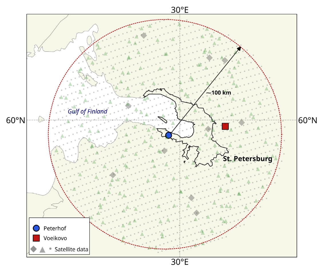
2.1. Ground-Based Observations

TOC datasets derived by three ground-based instruments are used in this study. Dobson spectrophotometer and M-124 filter ozonometer (https://woudc.org (accessed on 10 January 2022)) [22] are located in Voeikovo (59.95°N, 30.71°E; ~20 km East from St. Petersburg center, Russia) while Bruker 125 HR spectrometer is operated in Peterhof (59.88°N, 29.83°E; ~25 km South-Southwest from St. Petersburg center). The positions of Peterhof and Voeikovo are illustrated in Figure 1. The settlements are separated by approximately 50 km and located on the west (Peterhof) and east (Voeikovo) from the relatively high source of anthropogenic gases and aerosols of the megacity St. Petersburg. Peterhof and Voeikovo are located in green areas (mixed forest, grasslands, others) and out of influence of highly urbanized territories with their industries and dense traffic.

Dobson and M-124 instruments measure TOC by a differential method. The method is based on the registration of incoming UV solar radiation from two or more spectral intervals inside a 290–350 nm spectral area. After that TOC can be estimated as a logarithm of the relation of the radiation with different wavelengths. Dobson spectrophotometer is a double quartz monochromator which isolates incoming UV radiation in the following pairs of intervals—305.5/325.4 nm, 311.45/332.4 nm, and 317.6/339.8 nm [23]. The observations are usually carried out by direct sun, an error of individual measurement does not exceed 1–2%. Dobson spectrophotometer No108, located in Voeikovo, is a reference instrument in the Roshydromet ozone monitoring network. This spectrophotometer (hereinafter named simply as Dobson) is calibrated every 4 years by WMOs reference instrument [28].

A filter ozonometer M-124 (hereinafter M-124) is the main observing instrument in the Roshydromet ozone monitoring network, thus M-124 ozonometer located in Voeikovo is continuously calibrated by the nearby Dobson instrument. Major merits of M-124 are the simplicity of its construction and usage. Measurements by this instrument in Voeikovo [28] have been carried out for more than 40 years using direct and diffused to zenith solar radiation. Total errors of TOC measurements by the M-124 are 2–5% depending on the radiance data and atmospheric conditions. TOC observations by the Dobson and M-124 instruments on the Voeikovo site are available for 2009–2020 and 1985–2020, respectively. In the current study, we use Dobson data as a reference to validate several measurement systems.

TOC observations by the Bruker 125 HR FTIR-spectrometer were started at the Faculty of Physics of St. Petersburg State University in Peterhof in 2009 [45]. In 2016, this instrument was certified at the IRWG-NDACC observational network. The retrieval of TOCs from spectral measurements in 9.6 μm ozone absorption band is performed using PROFFIT96 software [29,46]. The FTIR measurements are carried out at clear-sky conditions (approximately 70–90 days per year). The systematic and random errors of TOC data used in the current study (v.007 at https://www-air.larc.nasa.gov/missions/ndacc/data.html (accessed on 10 January 2022)) are ~3% and ~2%, respectively.

2.2. Satellite Observations

In the current study we implement Level 2 pixel-based TOC data obtained by three satellite instruments: OMI (Ozone Monitoring Instrument [47] on AURA satellite) and TROPOMI (TROPOspheric Monitoring Instrument [48] on Sentinel-5P satellite) use the RS method (reflected and scattered solar radiation) and IKFS-2 (on Meteor-M No2) uses TR method (thermal radiation) [49,50,51].

OMI measures reflected and scattered solar radiation in UV and visible ranges of wavelengths (270–500 nm) with a spectral resolution of 0.42–0.63 nm [52]. The instrument’s geometries are close to nadir. Its spatial resolutions are 13 × 24 in the nadir viewing with a 2600 km swatch width.

TROPOMI consists of four spectrometers also measuring reflected and scattered solar radiation in a wide range of wavelengths 270–2385 nm with a spectral resolution of 0.25–0.55 nm. TROPOMI‘s spatial resolution constitutes 5.5 × 3.5 km² (after 6 August 2019) with a 2600 km swatch width. The instrument can be used to measure ozone and other gases globally in the presence of solar radiation [53] (as OMI).

IKFS-2 measures outgoing IR radiation of the Earth in a spectral range of 5–15 µm (660–2000 cm⁻¹) with unapodized spectral resolution of approximately 0.7 cm⁻¹. An IKFS-2′s swatch width can be changed from 1000 to 2500 km having a spatial resolution of approximately 35 km [50]. For estimation of TOC from the observations of IR radiation, measured by IKFS-2, we use a method based on a combination of the principal components approach and artificial neural networks. Satellite’s zenith angle, observation’s coordinates, dates and the main components of the measured total spectrum and spectrum in an ozone absorption line were used as predictors [49].

In

Table 1. Characteristics of the measurement instruments.

Instrument	Method	Horizontal Resolution, km	TOC Retrieval Error, %	Period of Observations Used
Bruker 125 HR	direct IR solar radiation	10–30, depending on solar zenith angle	2–3	2009–2020
Dobson	direct and scattered UV solar radiation	10–100, depending on solar zenith angle	1–2	2009–2020
M-124			3–5	1985–2020
IKFS-2	TR *	35 × 35	3–4	2015–2020
OMI	RS *	24 × 13	1–2	2004–2021
TROPOMI		7 × 3	<2–3	2018–2021

* TR—thermal radiation, RS—reflected and scattered.

the main characteristics (observation method, horizontal resolution, measurement errors, etc.) of the ground-based and satellite instruments used in this study are provided. The measurement errors of TOC are in a wide range (1–5%). They depend on such factors as measurements of radiation, atmospheric conditions, and quality of a priori information used. It should be noted that an analysis of the satellite TOC data is limited by the period of TROPOMI observations which have been started first in 2017.

The TOC measurements by Dobson and M-124 in Voeikovo and FTIR Bruker 125 HR in Peterhof are the only ground-based observations which are carried out regularly on the territory of St. Petersburg and its suburbs for the long time period (over 10 years). On top of that, the TOC retrieval in Voeikovo and Peterhof are based on two different methods (Table 1). All three datasets provide unique information on TOC variability in St. Petersburg independently. In their turn the satellites provide independent information on TOC variation in St. Petersburg with relatively high spatial resolution which is also based on two different retrieval methods. Hence, all the datasets of TOC measured near St. Petersburg are based on two different measurement techniques and four distinctive retrieval methods. Their comparison to the reference data is of great interest and that is why we use all of these datasets in the current study.

2.3. Model Data

TOC data from two chemistry-climate models (EMAC and INM RAS-RSHU) and two reanalysis datasets (ERA5 and EAC4) are used in this study.

ERA5 [54] data are global reanalysis of meteorological parameters and atmospheric composition for the period from 1950 to the present time. The reanalysis is prepared using global atmospheric transport model IFS (Integrated Forecasting System, version CY41R2) and an algorithm of observation data assimilation 4DVAR. A parametrization of TOC dynamic is based on a method which initially was presented in [55] and used in the climatic model ARPEGE of the France meteorological agency. Satellite measurements of TOC (e.g., MLS, OMI, SBUV, GOME, GOME-2, etc. [56]) are assimilated in ERA5. Spatial horizontal resolution is 0.25° (about 30 km) with vertical distribution on 137 hybrid levels up to ~80 km.

EAC4 is a global reanalysis of atmospheric composition which covers the time period from 2003 to the present day [57]. To generate the data, global chemistry-transport model (CTM) C-IFS (Integrated Forecasting System for Composition—IFS model which is coupled with CTM MOZART [58]) and 4DVAR observation assimilation algorithm are used. As in the case of the ERA5, satellite observations (SCIAMACHY, MIPAS, MLS, OMI, GOME-2 and SBUV/2) are also implemented to correct the model errors. EAC4 spatial resolution is a bit coarser than of ERA5 (0.75° or about 80 km). The data are distributed vertically on 60 hybrid levels up to ~70 km. ERA5 and EAC4 reanalysis data were obtained from https://cds.climate.copernicus.eu (accessed on 6 April 2022) and https://ads.atmosphere.copernicus.eu (accessed on 6 April 2022) respectively for a period from 2004–2021 with 3 h frequency.

Global CCM INM RAS-RSHU [59] is a combination of atmospheric (INM RAS General Circulation Model) and chemistry (RSHU) models. Its horizontal spatial resolution is 4 × 5° (~300 × 400 km² near the territory of interest) with vertical distribution on 39 hybrid levels up to approximately 90 km. The INM RAS-RSHU model treats about 74 chemically active gases in the lower and middle atmosphere which take part in 174 gas-phase and heterogeneous chemical reactions and in 51 photochemical reactions.

The second global CCM is ECHAM/MESSY Atmospheric Chemistry (EMAC) [60]. For this study an EMAC (ECHAM5 version 5.3.02, MESSy version 2.53) simulation was performed from 2002 to 2019 with a horizontal spatial resolution of 2.8° × 2.8° on 90 hybrid vertical levels up to approximately 80 km. The meteorology of the simulation was nudged towards ECMWF ERA-Interim re-analyses. The EMAC model simulates dynamical and chemical atmospheric processes which take place in the lower and middle atmosphere. The chemistry used includes 135 gaseous species and 298 chemical reactions and photolysis including heterogeneous reactions.

Table 2. Characteristics of the simulated data.

Data	Horizontal Resolution	Vertical Resolution	Time Coverage and Frequency	Assimilation of Meteorological Measurements	Assimilation of Ozone Measurements
ERA5	Hor. 0.25° (~31 km)	up to ~0.01 hPa (~80 km)	1979–2021, 3 h	Yes (in situ, satellite, radiosonde, radar data, etc.)	Yes (TOC, partial column, and profiles)
EAC4	Hor. 0.75° (~80 km)	up to ~0.1 hPa (~70 km)	2003–2021, 3 h	Yes (in situ, satellite, radiosonde, radar data, etc.)	Yes (TOC, partial column, and profiles)
INM RAS—RSHU	Hor. 4 × 5° (~300 × 400 km2)	up to ~90 km	2004–2021, 6 h	Yes (nudging of meteorological parameters)	No
EMAC	Hor. 2.8° (~155 km)	up to ~0.01 hPa (~80 km)	2002–2019, 1 h	Yes (nudging of meteorological parameters)	No

. includes several main characteristics of the simulated data used in this study.

3. Results and Discussion

3.1. Comparison of TOC Observations near St. Petersburg

For the comparison of the TOC data according to the different datasets we use a daily averaging procedure since the ground-based data are available as daily averages. The averaging is performed in Python by Pandas dataframe resample (‘1D’) mean function. All available TOC data of three satellite instruments are collected in a 100 km radius around St. Petersburg (Figure 1). We use the 100 km radius since it is the largest distance between Peterhof and ground-based measurement footprints (Table 1). On top of that, TROPOMI and OMI data are filtered by their quality flags (0 for OMI and >0.5 for TROPOMI). In the case of the satellite observations, the data are averaged in space as well since the daily satellite data cover Earth globally and provide plenty of the measurements in the 100 km radius from Peterhof (St. Petersburg) (Figure 1). Dobson TOC data retrieved only by direct radiation are used in the study. However, original M-124 data are not separated on TOC values which are retrieved by direct or scattered radiation. Nevertheless, the M-124 ozonometer in Voeikovo is regularly calibrated by the Dobson measurements. The data analysis is provided for several time spans in the 2009–2020 period. We do not compare all available datasets together for the one period due to a small number of data pairs (no more than 30). Hence, we separate the observation data by the following groups: Bruker 125 HR—M124—Dobson (2009–2020), Bruker 125 HR—M124—IKFS2—OMI (2015–2020), Bruker 125 HR—M124—TROPOMI (2018–2020), Dobson—IKFS2—OMI (2015–2020), Dobson—TROPOMI (2018–2020), IKFS2—OMI—TROPOMI (2018–2020).

Before the analysis, we present

Table 3. Statistical characteristics of the differences between TOC observation data near St. Petersburg for several time spans in the 2004–2020 period. MD and SDD of the difference relatively to Dobson mean TOC are shown in %. Letters in the cells mark different time spans in which the data are compared (a: 2009–2020, b: 2015–2020, c: 2018–2020, d: 2015–2020, e: 2018–2020, f: 2018–2020).

Instrument	Bruker 125 HR	M-124	Dobson	IKFS-2	OMI	TROPOMI
Bruker 125 HR	-	3.9/3.2 a	3.9/2.8 a	6.4/3.3 b	5.3/2.2 b	3.5/1.5 c
M-124	−3.9/3.2 a	-	0.0/2.3 a	2.6/4.3 b	1.6/3.3 b	0.9/3.6 c
Dobson	−3.9/2.8 a	0.0/2.3 a	-	2.4/3.6 d	1.8/3.3 d	2.2/3.7 e
IKFS-2	−6.4/3.3 b	−2.6/4.3 b	−2.4/3.6 d	-	−0.7/3.1 f	−2.1/3.2 f
OMI	−5.3/2.2 b	−1.6/3.3 b	−1.8/3.3 d	0.7/3.1 f	-	−1.4/2.1 f
TROPOMI	−3.5/1.5 c	−0.9/3.6 c	−2.2/3.7 e	2.1/3.2 f	1.4/2.1 f	-

and

Table 4. Natural TOC variability in DU for all observation data near St. Petersburg for time spans in the 2004–2020 period (as a standard deviation of the mean) in DU; letters in cells mark different time spans in which the data are compared (a: 2009–2020, b: 2015–2020, c: 2018–2020, d: 2015–2020, e: 2018–2020, f: 2018–2020).

Instrument	Bruker 125 HR	M-124	Dobson	IKFS-2	OMI	TROPOMI
Bruker 125 HR	-	48.5/45.3 a	48.5/46.2 a	58.9/54.5 b	58.9/55.9 b	46.3/45.8 c
M-124	45.3/48.5 a	-	45.3/46.2 a	54.4/54.5 b	54.3/55.9 b	44.6/45.8 c
Dobson	46.2/48.5 a	46.2/45.3 a	-	46.5/47.2 d	46.5/48.0 d	40.2/41.0 e
IKFS-2	54.5/58.9 b	54.5/54.4 b	47.2/46.5 d	-	44.8/47.4 f	44.8/47.6 f
OMI	55.9/58.9 b	55.9/54.3 b	48.0/46.5 d	47.4/44.8 f	-	47.4/47.6 f
TROPOMI	45.8/46.3 c	45.8/44.6 c	41.0/40.2 e	47.6/44.8 f	47.6/47.4 f	-

which contain statistical characteristics of the differences. Table 3 contains the mean difference (MD) and standard deviation of the difference (SDD)—between daily-averaged ground-based and satellite TOC data near St. Petersburg for several time spans. Table 4 contains information on natural TOC variability which is found as standard deviation of the mean and characterizes TOC variation caused by all factors (atmospheric circulation, anthropogenic activity, solar activity, volcanic eruptions, and others). In the tables, the compared datasets are labeled with letters depicting the period used for the comparison. It should be noted, even though some different letters apply to the same year coverage (e.g., “b” and “d”, 2015–2020), they are for different time spans. This is because, for example, ground-based and satellite data covered a high number of days in a particular year when they did not overlap each other. That usually results in a different number of the daily averaged measurements in that year.

3.1.1. Ground-Based Observations

Daily mean TOC data derived by Bruker 125 HR and M-124 correlate well (Pearson’s correlation coefficients are 0.98–0.99) with Dobson (reference) data for the 2009–2020 period (about 270 days) (Figure 2). However, Bruker TOCs have relatively high MDs with two other datasets—in a range 12.6–12.9 DU (3.9%) (see Table 3). SDDs constitute about 9.3 DU (2.8%) and 10.6 DU (3.2%) for Dobson-Bruker and M-124—Bruker data pairs, respectively. M-124 and Dobson data fit better having MD and SDD of 0.0 and 2.3%. This is probably related to the periodical calibration of M-124 by Dobson which are both located at the same station in Voeikovo (Figure 1). Figure 2 presents the time series of TOCs for all three instruments and their differences with respect to Dobson data. TOC seasonality can be clearly seen in this graph with the maximum values in spring and the minimum in the early autumn. The TOCs vary in a range from 250 to about 540 DU. The yearly TOC minima usually are in a range of 275–300 DU when the maxima are more variable—400–540 DU. However, it can be partly explained by the fact that the period from 2009 to 2020 is not covered equally by the data since there can be different numbers of measurements in particular years and months. Natural variability in TOCs is nearly the same for all datasets (45.3–48.5 DU, Table 4).

The results of the first preliminary analysis of TOC measurements, derived using Bruker 125 HR in Peterhof, and comparison with different datasets were presented in a study [61] where the first measured 269 spectra (52 days, from March to November 2009) were processed. MD and SDD between Bruker and Dobson data for 17 days were 0.3 and 3.2%. MD and SDD between Bruker and M-124 data on average constituted 0.4 and 3.4%. Next comparison was performed using 1190 spectra measured by Bruker 125 HR during 189 days in a period from April 2009 to March 2012. It was found that MD and SDD between Bruker 125 HR and Dobson were 1.4 and 3.4% (74 days). MD and SDD between Bruker and M-124 were 2.8 and 3.9% (78 days). In the study [22] three datasets during different time spans were compared. The research demonstrated that MDs and SDDs between the Bruker 125 HR, M-124 and Dobson data varied in a range of 1.6–2.2 and 2.3–2.9%. It means that TOCs in Peterhof and Voeikovo (~50 km apart) can differ noticeably depending on the analyzing time span which characterizes spatial-temporal variations in ozone in the atmosphere above both stations.

Apart from dynamical variation in air masses in a spring season when TOC can change by 20–30% at one station throughout the day (see for example [62]), variations in tropospheric ozone content, which is only ~10% of TOC, may be another reason for the differences in TOC measured at Voeikovo and Peterhof stations. St. Petersburg is a large anthropogenic source of gases and aerosols and depending on wind direction it can influence tropospheric ozone content at both stations. An analysis of surface wind direction at the Peterhof site showed that Voeikovo station, which is on the east of city St. Petersburg, is more often under anthropogenic influence of the city than Peterhof, which is on the south-west of St. Petersburg. By contrast, in Peterhof air masses with fewer anthropogenic influence should prevail. That is why higher content of NO_x (NO and NO₂) at Voeikovo can lead to noticeable variability in tropospheric ozone content at this station (and, as a result, in TOC) since NO_x molecules participate in the formation and destruction of ozone [2]. The variability in tropospheric ozone can also be caused by such natural sources as chemical reactions with hydrocarbons which are emitted by vegetation (e.g., oxidation of CH₄ and NMHC by OH) [63]. However, since Voeikovo and Peterhof are located in quite similar conditions, surrounded by mixed forest and grasslands, the difference between the Voeikovo and Peterhof TOC should minimize the influence of the natural factor. In addition, overestimation of TOC by Bruker 125 HR in comparison to Dobson and M-124 measurements can be caused by differences in IR and UV spectroscopic information which is used for the interpretation of the measured solar radiation.

TOC observations by Bruker 125 HR and Brewer instruments at Izana station (Tenerife, Spain) were compared in [64]. The Bruker spectrometer overestimated TOC measured by the Brewer instrument on average by 4–4.9 with SDD of 1%. Authors suggested that the high MDs could be caused by several reasons. These are simplified algorithms used for the interpretation of solar radiation measured by the Brewer, discrepancies in IR and UV absorption coefficients and errors in determination of the instruments’ characteristics. Similar results were presented in [65] where TOC observations at the Izana station measured by Bruker 125 HR and Brewer were also compared. In this study MD and SDD between the measurement data constitute 4.2 and 0.7%. Authors mention that the possible reason for such a high average difference could be discrepancies in spectroscopic parameters (e.g., differences in IR and UV absorption coefficients). It is highlighted that HITRAN absorption line intensities and absorption cross-sections of Bass and Paur were used to interpret the Bruker and Brewer data, respectively.

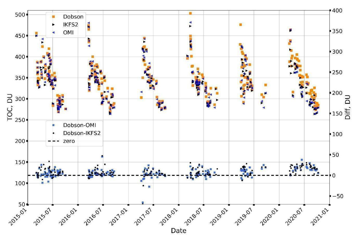
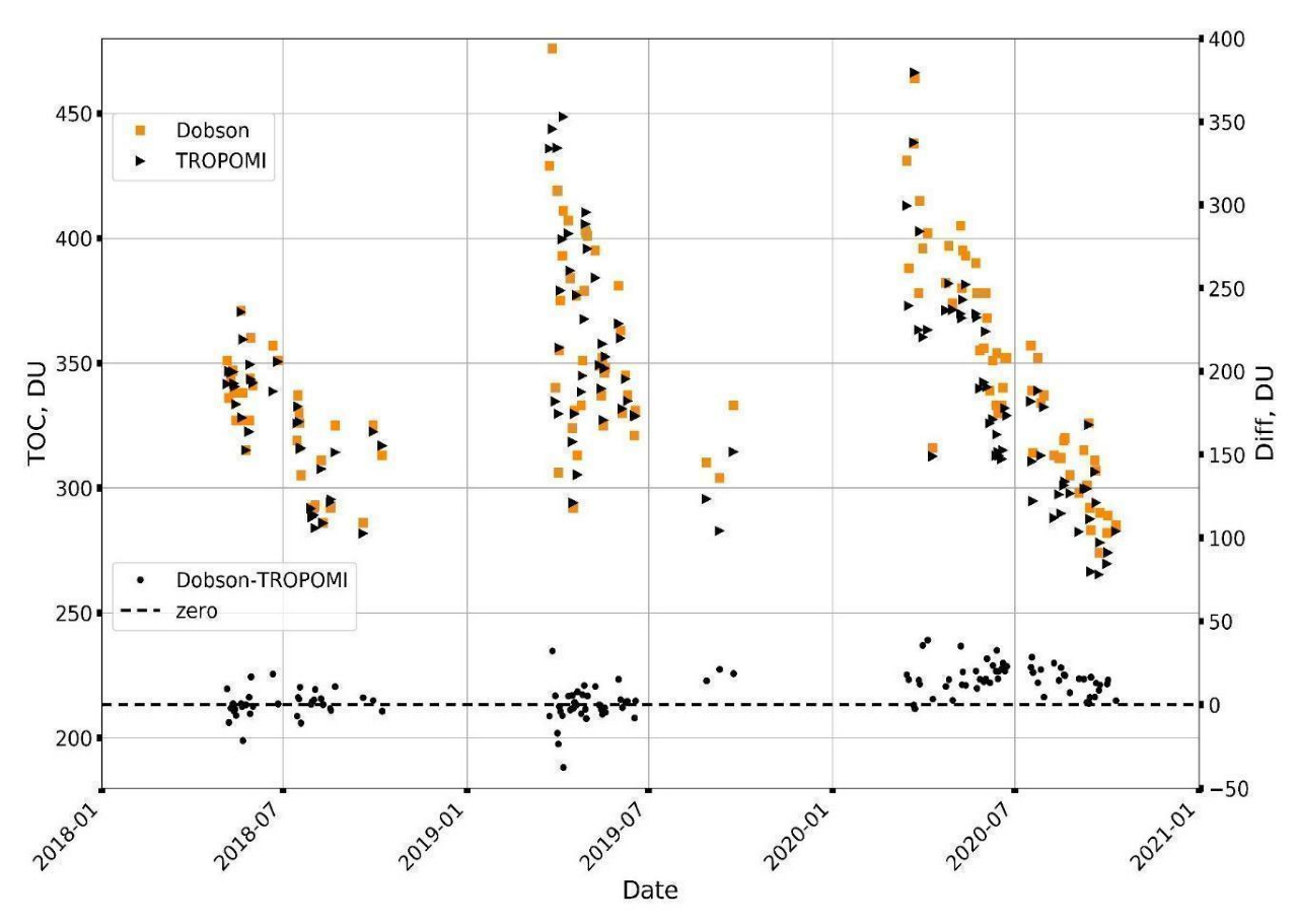
3.1.2. Satellite and Dobson Observations

Comparison of the Dobson data with the IKFS-2 and OMI satellite TOC measurements near St. Petersburg for the 2015–2020 period (143 days) reveals a quite good fit in their time series (Figure 3) with a correlation coefficient of 0.97. In addition, natural TOC variances of the datasets (SDD of the mean) are in good agreement (about 46–48 DU, Table 4). On average, TOC values measured by the satellites are smaller than by the ground-based instruments. The OMI and Dobson data are in a slightly better agreement than IKFS-2 and Dobson. MDs and SDDs constitute 1.8 and 3.2% for Dobson-OMI, 2.4 and 3.6% for Dobson-IKFS-2 (see Table 3).

IKFS-2 TOC measurements and ground-based data (Dobson and Brewer) derived at stations from different parts of the Earth for a 2019–2020 period were analyzed in [49]. It was shown that MDs and SDDs between the satellite and ground-based observations were approximately −1.5 and 2.6%, provided that maximal spatial and temporal mismatches between the measurements were less than 70 km and 1 h, respectively. It should be noted that the mean differences between the IKFS-2 and Dobson data, which we found in the current study, are a bit higher (with MD and SDD of 2.4 and 3.6%) than in [49]. This can be due to larger spatial and temporal observation mismatches which we use (100 km and 24 h vs. 70 km and 1 h).

An analysis of the TROPOMI and Dobson data near St. Petersburg for a 2018–2020 period shows that they are close in TOC time series (correlation coefficient of 0.96, based on 130 days of data, see Figure 4). MD and SDD are 2.2 and 3.7% which are almost the same as in the case of the IKFS-2 and Dobson comparison (Table 3). However, these values cannot be compared directly since the TROPOMI and IKFS-2 data cover different time spans (2018–2020 and 2015–2020, respectively).

3.1.3. Satellite Observations

All three satellite TOCs datasets for a 2018–2020 period are in good agreement (Figure 5). Correlation between the datasets is about 0.98–0.99 with natural variability of 44–48 DU (Table 4). MDs and SDDs between the data are in a range 0.7–2.1 and 2.1–3.2% (Table 3). The smallest MD is for the pair IKFS-2-OMI (0.7%). It is due to the implementation of the OMI data in training the artificial neural network which was used in the interpretation of IR spectra measured by IKFS-2 [49]. However, the smallest SDD is between the OMI and TROPOMI data (about 2.1%) which can be caused by higher spatial resolution of the TROPOMI data than of IKFS-2 (~7 × 3 vs. 35 × 35 km²). In a study [66] authors compare ground-based TOC measurements by Brewer instruments at three stations in Antarctica with Level 2 and 3 satellite data by OMI, TROPOMI, OMPS (Suomi NPP), AIRS (Aqua) and GOME-2 (MetOp-B). They demonstrate that the Level 2 satellite data with higher spatial resolution (TROPOMI—7 × 7, 5 × 3.5 km²; OMI −13 × 24, 13 × 12 km²) fit the ground-based observations in Antarctica better than with cruder resolution (OMPS—50 × 50 km², AIRS—50 × 50 km², GOME-2—40 × 40 km²). For example, the smallest MDs and SDDs are for TROPOMI and OMI (0.1–8.6 and 7.5–18.1 DU) when the largest—for OMPS and AIRS (1–24 and 16.5–44.3 DU). Note that, the GOME-2 data, whose spatial resolution is 40 × 40 km², fit the ground-based observations better than OMPS and AIRS (MDs and SDDs are 2.8–10.1 and 14.6–20.1 DU). In addition, larger SDD between the IKFS-2 and OMI data in our study can be related to the differences in spectroscopic characteristics and ozone retrieval algorithms of two different techniques of TOC estimation (TR and RS, see Table 1).

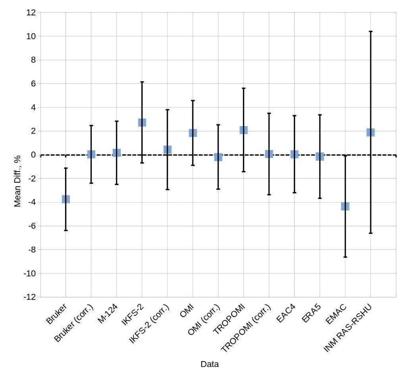
3.1.4. Satellite and Ground-Based (Bruker 125 HR and M-124) Observations

TOC data observed by the Bruker 125 HR and M-124 ground-based measurements correlate well with the IKFS-2 and OMI satellite observations for the 2015–2020 period with correlation coefficients of 0.97–0.99 and natural variance of 54–59 DU (Table 4). MDs and SDDs between the ground-based and satellite data are 5.3–6.4 and 2–3% and 1.6–2.6 and 3.3–4.3% for the Bruker 125 HR and M-124, respectively (Table 3). The smaller MDs between the M-124 and satellite measurements can be related to the fact that OMI (and, as a result, IKFS-2) and M-124 are calibrated by ground-based Dobson data. However, the SDDs are smaller in the case of the Bruker 125 HR, which can be due to the significantly better spectroscopic characteristics of this instrument in comparison to the M-124.

As in all previous cases, TOC measured by Bruker 125 HR and M-124 correlated well with the TROPOMI data for the 2018–2020 period (correlation coefficient was 0.99, 120 days). MDs and SDDs between two ground-based instruments and TROPOMI data constitute 3.5 and 1.5% (Bruker 125 HR), 0.9 and 3.6% (M-124). In general, all satellite data underestimate TOC measured by the ground-based instruments.

3.2. Correction of TOC Measurements

As it was shown above, the TOC data derived by different measurement systems (ground-based and satellite) on average differ with the Dobson measurements by 0.0–3.9 and with SDDs by 2.3–3.7%. The datasets analyzed in this research, are available for different time spans (different number of the TOC measurements per year). Moreover, only some of them overlap each other for relatively long time periods (e.g., the Bruker 125 HR, Dobson and M124 data—from 2009 to 2020). We suppose that harmonization of the data (i.e., correction to the reference) can solve at least two issues. At first it can fill gaps in long-term TOC variations near St. Petersburg. Secondly, the harmonized data can be used to evaluate long-term TOC trends. For example, in [67] authors adjust the TOC observations by different satellites to ground-based Dobson data at Halley station (Antarctic) subtracting the Dobson-Satellite Data mean differences.

Here we use a simple method of the correction which was proposed in [68]. In the method it is supposed that the reference data (Dobson) can be estimated by linear regression

$$x_{1i}=a+b\ast x_{2i}$$

(1)

where $x_{2i }$—the data which are going to be corrected by the reference ($x_{1i}$); a and b—coefficients which can be found by the following equations:

$$b={\displaystyle \sum }_{i=1}^n\frac{\left(x_{1i}-{\overline{x}}_1\right)\left(x_{2i}-{\overline{x}}_2\right)}{{\sum }_{i=1}^n{\left(x_{2i}-{\overline{x}}_2\right)}^2}$$

(2)

$$a={\overline{x}}_1-b\ast {\overline{x}}_2$$

(3)

where ${\overline{x}}_{1,2}$—reference and corrected data means, respectively.

We applied the correction to all measurement data except M-124. The statistical characteristics of differences between the corrected data are given in

Table 5. Statistical characteristics of differences between corrected TOC observation data near St. Petersburg for several time spans in the 2004–2020 period. MD and SDD relatively to Dobson mean TOC are shown in %. Letters in cells depict different time spans in which the data are compared (a: 2009–2020, b: 2015–2020, c: 2018–2020, d: 2015–2020, e: 2018–2020, f: 2018–2020).

Instrument	Bruker 125 HRcorr	M-124	Dobson	IKFS-2corr	OMIcorr	TROPOMIcorr
Bruker 125 HRcorr	-	−0.1/2.9 a	0.1/2.6 a	0.0/2.8 b	−0.7/1.8 b	−2.3/1.4 c
M-124	0.1/2.9 a	-	0.0/2.3 a	0.3/4.3 b	−0.5/3.2 b	−1.3/3.5 c
Dobson	−0.1/2.6 a	0.0/2.3 a	-	0.1/3.6 d	−0.3/3.2 d	0.1/3.6 e
IKFS-2corr	0.0/2.8 b	−0.3/4.3 b	−0.1/3.6 d	-	−0.4/3.0 f	−1.7/2.9 f
OMIcorr	0.7/1.8 b	0.5/3.2 b	0.3/3.2 d	0.4/3.0 f	-	−1.3/2.0 f
TROPOMIcorr	2.3/1.4 c	1.3/3.5 c	−0.1/3.6 e	1.7/2.9 f	1.3/2.0 f	-

. The correction led to significant decrease of the mean (systematic) differences, which in general do not exceed 0.5%. The SDDs were also slightly reduced after the correction (by 0.1–0.4%). It can be noticed that this procedure insignificantly improved the differences between TROPOMI and other datasets. In addition, the MD between the TROPOMI and M-124 measurements increased by 2.2% (from 0.9 to −1.3%) after the correction. However, the difference between the TROPOMI and Dobson data also decreased down to approximately 0%. Finally, TOC values according to the corrected satellite measurements in general overestimate the ground-based data when there was an opposite situation before the correction.

3.3. Comparison of TOC Observations and Modelled Data

To compare the simulated and observed TOC near St. Petersburg at first all the modelled data are exported from a model cell which covers the territory of the city. Secondly, daily averages of the simulated TOC are found in the same way as for the observations (see Section 3.1). Here we compare all the simulated data with each other as well as to the ground-based and satellite observations. Hence, only three groups of the data were analyzed: Simulated data—Simulated data (2004–2019), Bruker 125 HR—M124—Dobson—Simulated data (2009–2019) and OMI—TROPOMI—IKFS2—Simulated data (2018–2019).

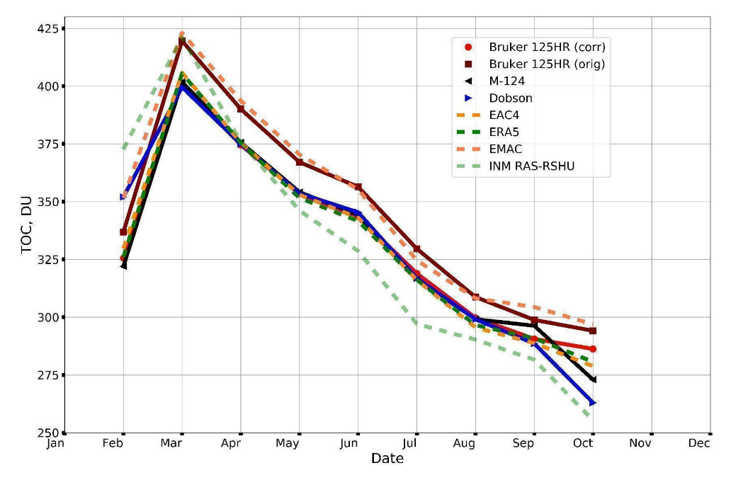
3.3.1. Ground-Based Observations and Modelling

The main statistical characteristics of the difference between the observed and simulated TOC (before and after the correction) are given in

Table 6. Statistical characteristics of differences between original observed and simulated TOC near St. Petersburg for several time spans in the 2004–2019 period. MD and SDD relatively to Dobson mean TOC are shown in %. Letters in cells depict different time spans in which the data are compared (a: 2009–2019, b: 2018–2019, c: 2004–2019).

Instrument	Bruker 125 HR	М-124	Dobson	IKFS-2	OMI	TROPOMI	ERA5	EAC4	EMAC
ERA5	−4.2/2.4 a	−0.4/3.7 a	−0.2/3.9 a	3.9/3.3 b	2.9/2.7 b	1.5/2.0 b	-	0.8/1.7 c	−2.9/3.6 c
EAC4	−4.1/2.2 a	−0.3/3.4 a	−0.1/3.7 a	2.8/3.3 b	1.8/2.7 b	0.4/2.0 b	−0.8/1.7 c	-	−3.6/3.2 c
EMAC	0.5/3.7 a	4.3/4.3 a	4.5/4.5 a	5.0/4.1 b	3.9/4.2 b	2.6/3.8 b	2.9/3.6 c	3.6/3.2 c	-
INM RAS—RSHU	−5.4/8.5 a	−1.6/8.6 a	−1.4/8.6 a	−1.2/8.3 b	−2.3/8.6 b	−3.6/8.4 b	−2.3/8.7 c	−1.5/8.7 c	−5.1/7.8 c

and

Table 7. Statistical characteristics of differences between corrected observed and simulated TOC near St. Petersburg for several time spans in the 2004–2019 period. MD and SDD relatively to Dobson mean TOC are shown in %. Letters in cells depict different time spans in which the data are compared (a: 2009–2019, b: 2018–2019, c: 2004–2019).

Instrument	Bruker 125 HR	М-124	Dobson	IKFS-2	OMI	TROPOMI	ERA5	EAC4	EMAC
ERA5	−0.2/2.3 a	−0.4/3.7 a	−0.2/3.9 a	1.4/3.4 b	0.7/2.6 b	−0.6/1.9 b	-	0.8/1.7 c	−2.9/3.6 c
EAC4	−0.1/2.1 a	−0.3/3.4 a	−0.1/3.7 a	0.3/3.3 b	−0.4/2.7 b	−1.7/2.0 b	−0.8/1.7 c	-	−3.6/3.2 c
EMAC	4.5/3.5 a	4.3/4.3 a	4.5/4.5 a	2.4/4.0 b	1.7/4.1 b	0.4/3.5 b	2.9/3.6 c	3.6/3.2 c	-
INM RAS—RSHU	−1.4/8.4 a	−1.6/8.6 a	−1.4/8.6 a	−3.8/8.2 b	−4.5/8.4 b	−5.8/8.1 b	−2.3/8.7 c	−1.5/8.7 c	−5.1/7.8 c

.

Both reanalysis datasets (EAC4 and ERA5) fit relatively well with each other with MD and SDD of 0.8 and 1.7% (Table 6). By contrast, the reanalysis data noticeably deviates from the EMAC and INM RAS-RSHU results. For example, the EMAC data on average overestimate TOC in relation to the ERA5 by 2.9 with SDD of 3.6% and to the EAC4 by 3.6 with SDD of 3.2%. However, the INM RAS-RSHU simulated data in general underestimate the reanalysis with MDs and SDDs of −2.3 and 8.7% (ERA5), −1.5 and 8.7% (EAC4). The INM RAS-RSHU data have a closer fit on average with the reanalysis but also shows very large SDDs (about 8.7%). Finally, the EMAC data set differs from INM RAS-RSHU on average by 5.1 with SDD of 7.8%.

For the 2009–2019 period, reanalysis data match the Dobson and M-124 ground-based observations quite well with MDs of ~0% and SDDs of 3.4–3.9% (Table 6). The differences between the ERA5 (EAC4) reanalysis data and Bruker 125 HR measurements before and after the correction changed from 4.2% (4.1%) to −0.2% (−0.1%). However, the SDD between the Bruker and reanalysis is the minimal and constitutes about 2%. The EMAC model on average significantly overestimates the ground-based Dobson and M-124 TOC values by about 4.5% and 4.3% while the INM RAS-RSHU underestimates them by −1.4% and −1.6%. MDs between Bruker 125 HR and CCMs data before and after the correction changes from 0.5 to 4.5% for EMAC and from −5.4 to −1.4% for INM RAS-RSHU (Table 6 and Table 7, respectively). The EMAC fit the corrected Bruker measurements worse when the opposite situation is for the INM RAS-RSHU. In contrast, SDDs between the INM RAS-RSHU and ground-based observations are the maximal and constitute 8.5–8.6% while they are 3.7–4.5% for EMAC. Nevertheless, all the simulated data correlate noticeably well with the ground-based observations at monthly, seasonal, and annual time scales with the correlation coefficients of 0.82–0.99. The smallest coefficients are for INM RAS-RSHU (0.82–0.83), then for EMAC (0.94–0.96), and finally for ERA5 and EAC4 (0.96–0.99). The measured natural TOC variability (44–46 DU, SDD of the mean) is depicted well by the models and constitutes 45–49 DU (49 DU for INM RAS-RSHU).

Simulated and ground-based TOCs have a pronounced seasonal variability (Figure 6) with the maximum in March (~400–425 DU) and the minimum in October (~260–300 DU). An absence of the data for some months on the graph is due to the fact that some observations are carried out during specific periods in a year. For example, TOC measurements by the Dobson in Voeikovo are not provided in November–January. The EMAC and INM RAS-RSHU differ with the ground measurements significantly (by 10–25 DU). However, the difference between the observations and EMAC is almost stable while the difference between the observations and the INM RAS-RSHU data varies from almost 0 (April–May) to 25 DU (March and July) depending on the month. The amplitude of the TOC variability is quite high, reaching approximately 125 DU. The TOC seasonal variability and amplitude here fit well with the results of independent studies. For example, in [69] a TOC seasonal variation for latitude of St. Petersburg, which is based on satellite data GOME-type Total Ozone Essential Climate Variable (GTO-ECV) and reanalysis Adjusted-MERRA, for a 1995–2018 period also has the maximum in the beginning of spring (420 DU) and the minimum in autumn (310 DU). Figure 6 shows a good match between the reanalysis and ground-based observations.

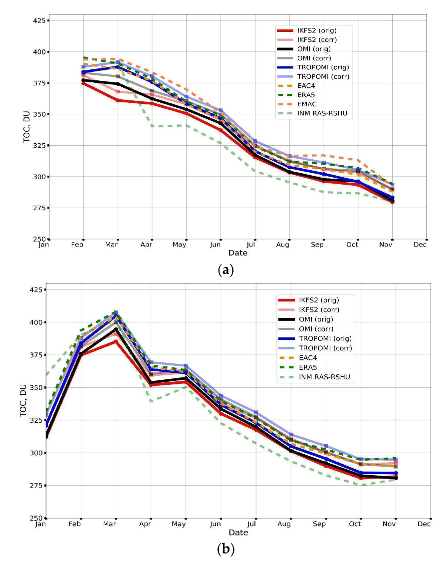
3.3.2. Satellite Observations and Modelling

The reanalysis data on average overestimate the original TOC satellite measurements by 0.4–3.9 with SDDs of 2.0–3.3% for the 2018–2019 period (see Table 6). The EMAC model overestimates the satellite data significantly with the MDs and SDDs up to 2.6–5.0 and 3.8–4.2%. The INM RAS-RSHU underestimates satellite observations by −1.2 to −3.6% but with the maximal SDDs (8.3–8.6%). The correction of the satellite observations (see Table 7) reduced the MDs for the reanalysis (0.3–1.7%) and EMAC simulated data (0.4–2.4%). However, the MDs between corrected satellite observations and INM RAS-RSHU increased by −3.8 to −5.8%.

Despite the higher spatial resolution of the ERA5 compared to EAC4 data (approximately 31 vs. 80 km), EAC4 TOC reanalysis matches the satellite measurements better (by about 1%). The best agreement was found between the EAC4 and original TROPOMI data (with MD and SDD of 0.4 and 2.0%). In general, the simulated data correlate well with the satellite observations with the correlation coefficients varying in a range of 0.78–0.99 (0.97–0.99 for the reanalysis, 0.94–0.96 for the EMAC, 0.78–0.80 for the INM RAS-RSHU). The natural TOC variability derived from the modelled data fits the observations relatively well with the values in a range 40–44 DU.

Figure 7 depicts the seasonal variability in the TOCs near St. Petersburg derived from satellite observations and simulated data with (a) and without (b) EMAC. We present the seasonal variability with and without EMAC data because their inclusion reduces the length of the data series. This leads to the noticeable differences with the TOC seasonal variation from the ground-based measurements (Figure 6). Figure 7 demonstrates good agreement between the TOC seasonal variability in simulated data and satellite measurements. The TOC seasonal variability derived from the satellite data is very pronounced and quite similar to that in ground-based data (Figure 6 and Figure 7b). The maximum (390–410 DU) and minimum (280–290 DU) are also registered in March and October-November, respectively. The graph with the EMAC data included (Figure 7a) represents that TOC seasonal variability has distinctive features in the period from February to April—absence of the temporal TOC growth. And again, the worst agreement between the measured and simulated TOC seasonal variability was found for EMAC and INM RAS-RSHU.

Note that differences between TOC seasonal means derived from the different observation systems and simulated data (Figure 6 and Figure 7) reach in some months approximately 25 DU which is noticeably higher than recommended measurement errors of 2–3% [70].

To conclude the analysis, we provide the graph which depicts MDs of all TOC data related to Dobson reference observations (Figure 8). As opposed to the previous analysis, where we separated the data into several groups with the different time spans, here we compare the TOC datasets with Dobson measurements individually using every available pair of “Reference-Not reference”. In Figure 8, a vertical axis is for MDs (Dobson instrument minus data from the other sources), vertical bars for SDDs of the differences and symbols stand for each TOC dataset. The analysis was carried out for the original and corrected data.

The original TOC observation data (except for M-124 ground-based measurements) and EMAC and INM RAS-RSHU simulated data differ from the Dobson measurements on average by 2% and more. The maximal MDs are for the original Bruker 125 HR measurements and EMAC simulated data (approximately 4%). The minimal differences (less than 0.5%) are for M-124 observations, corrected observation data and reanalysis. Almost all TOC datasets have SDDs which vary in a range 2.6–3.5%. However, the INM RAS-RSHU and EMAC simulated data have larger SDDs which constitute 8.5 and 4.3%, respectively. This is probably due to coarse spatial resolution of these simulated data (2.8–5°) and, as a result, a lack of ability to consider local small-scale atmospheric processes and detailed spatial distribution of gas and aerosol emissions on the territory of St. Petersburg megacity. By contrast, the noticeably good agreement between the reanalysis (EAC4 and ERA5) and Dobson data may be caused by the assimilation of TOC observations.

3.4. Analysis of TOC Trend near St. Petersburg

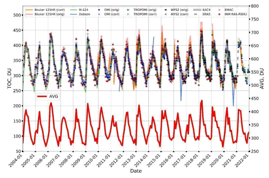
3.4.1. Variations in Monthly Averaged TOC

Figure 9 depicts time series of monthly averaged TOC values derived from all observations (original and corrected) and modelling for the 2004–2021 period. In addition, the graph includes a full TOC average (shown as a red curve) which was calculated by averaging all datasets.

In general, all datasets are close to each other presenting similar interannual and seasonal TOC variations. The maximal monthly averaged values are for EMAC, INM RAS-RSHU and original Bruker 125 HR data (as it has been shown before). Dobson and corrected Bruker 125 HR monthly averaged data sometimes differ from the other datasets significantly (see for example 2017, 2019, 2021 in Figure 9). Most likely it is due to a different number of measurements for particular dataset in a specific month.

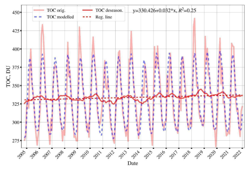
3.4.2. Estimation and Analysis of TOC Trend

To estimate the TOC trend near St. Petersburg from the long-term observations and modelling, the TOC seasonal behavior should be eliminated. The main factors impacting TOC variability are global atmospheric transport (e.g., Brewer-Dobson circulation), Quasi-Biennial Oscillation (QBO), El Niño/Southern Oscillation (ENSO), solar cycle, anthropogenic influence, and others. These processes and phenomena are of specific regularity. For example, QBO has a period of approximately 2 years, ENSO—~3 years, solar cycle—~11 years. Here we apply multi-linear regression (MLR) modelling which is described in [71]. The method assumes that there is a linear relationship between the TOC variation (a dependent variable) and the main influencing factors (independent variables or predictors). The MLR equation can be written in the following way:

$$TO{C}_M=Const+a\ast QBO+b\ast ENSO+c\ast Solar+d\ast t+$$

$${\displaystyle \sum }_n^N\left(e_n\ast sin\left(2\frac{\pi \ast t}{I_n}\right)+f_n\ast cos\left(2\frac{\pi \ast t}{I_n}\right)\right)$$

(4)

where $TO{C}_M$—modelled TOC; Const—constant; a–f—regression coefficients; QBO, ENSO, Solar—parameters representing the influence of QBO, El Niño, solar cycle, respectively; t—time vector; l_n—3, 4, 6 and 12 months. Constant and regression coefficients a–f were determined while solving the MLR using real TOC data, the predictors, and the least square method. Here we use total monthly averaged TOC data (Figure 9, red curve) as the dependent variable to create the MLR model. To include the impact of QBO we use zonal wind speed anomaly data at altitudes 30 and 50 mb in the equatorial zone (https://www.cpc.ncep.noaa.gov/data/indices/ (accessed on 15 April 2022)). Bi-monthly Multivariate El Niño/Southern Oscillation (ENSO) index (https://psl.noaa.gov/enso/mei/ (accessed on 15 April 2022)) is applied as ENSO predictor which is based on five climatological parameters for the equatorial zone of the Pacific Ocean—sea level pressure, sea surface temperature, zonal and meridional components of the surface wind, and outgoing longwave radiation. The solar cycle influence is described by solar radio flux at 10.7 cm wavelengths (https://spaceweather.gc.ca/forecast-prevision/solar-solaire/solarflux/sx-3-en.php (accessed on 15 April 2022)). Harmonic functions in the Equation (4) (sin and cos) include TOC variations with 3-, 4-, 6- and 12-month regularity. This part of the equation considers the influence of the Brewer-Dobson circulation (the TOC seasonality).

At the next stage we found all regression coefficients a–f using the Equation (4), calculated $TO{C}_M$ and subtracted a part which corresponds to the TOC seasonal variability i.e., ${\displaystyle {\sum }_n^N}\left(e_n\ast sin\left(2\frac{\pi \ast t}{I_n}\right)+f_n\ast cos\left(2\frac{\pi \ast t}{I_n}\right)\right).$ Accordingly, the deseasonalized TOC can be calculated as the following:

$$TO{C}_{M,Deseason.}=TO{C}_M-{\displaystyle \sum }_n^N\left(e_n\ast sin\left(2\frac{\pi \ast t}{I_n}\right)+f_n\ast cos\left(2\frac{\pi \ast t}{I_n}\right)\right)$$

(5)

Figure 10 shows the time series of the original TOC dataset, TOC modelled by the MLR method (Equation (4)), deseasonalized TOC (Equation (5)) and its linear regression with equation and coefficient of determination. The original and simulated TOC data are in good agreement having a correlation coefficient of 0.90. MD and SDD between the original and modelled TOC data constituted approximately 0 and 5.5%. The procedure of deseasonalization reduced the TOC natural variability (standard deviation of mean) significantly. For example, the simulated TOC natural variability before and after the deseasonalization are 38 and 3.9 DU, respectively (the original TOC natural variability constitutes 42 DU). Note that, the mean TOC did not change substantially (333 DU). The linear trend of the deseasonalized data shows a slight TOC increase of about 0.4 ± 0.1 DU per year near St. Petersburg for the 2004–2021 period. The trend’s uncertainty is calculated with reduced effect of the deseasonalized ozone data auto-correlation [72]. T-test with 0.95 confidence level revealed that the trend is significant (t = 8.3, t_critical = 1.97).

The analysis of the Equation (4) revealed that the 12- and 6-month harmonic functions influence the TOC variation most noticeably. The QBO, ENSO and solar cycle in general lead to a slight increase in the MD (up to 4%). The positive TOC trend is caused by the inclusion of the time vector to the MLR model which can depict such factors as CO₂ content increase, reduction of freons, volcanoes, etc.

4. Conclusions

In the current study we carried out the analysis of TOC variations near St. Petersburg for the time spans within the 2009–2021 period measured by ground-based and satellite instruments as well as from modelled data. The observations were performed by four different remote sensing methods which are based on measurements of downwelling solar radiation at the surface and outgoing radiation at the top of the atmosphere. The different properties of measurement systems, TOC retrieval algorithms, etc. cause the differences between TOC observations. In its turn, simulated TOC can also differ due to different spatial resolution, complexity of physical and chemical processes included, etc.

The analysis demonstrates that TOC variations measured by all observation systems are in good agreement with the correlation coefficients higher than 0.95. The mean differences (MDs) and their standard deviations between the pairs of measurements (SDDs) considered vary in a range 0.0–6.4 and 1.5–4.3%. The MDs between the measurements and reference data (Dobson instrument) constitute 0.0–3.9 with SDDs of 2.3–3.7% and are close to the modern requirements for TOC observations [71]. We have shown that all data can be harmonized to the standard measurements by the linear regression approach which almost reduces a systematic difference between measurements. Except for the differences in methods, instruments, and model characteristics, etc., results of such investigations strongly depend on the period analyzed and amount of available data. These facts highlight the importance of the development of ground-based ozone networks to ensure regular TOC observations (in time and space). This will help to provide more information on long-term ozone variability at a particular station and its surroundings which will increase robustness of satellite instruments validation.

In general, the modelled data reproduce TOC variations near St. Petersburg quite well with the best results for EAC4 and ERA5 reanalysis. It should be highlighted that the reanalysis data fit the reference measurements almost as good as the satellite observations. This may be due to assimilation of measurements to reanalysis data. For the particular regions we may recommend to use the EAC4 and ERA5 reanalysis data to fill gaps in measured TOC data series even at the daily time scales. In their turn, chemistry-climate models (CCM) cannot reproduce local dynamical and chemical processes on a scale of St. Petersburg having larger errors. CCMs are usually used to investigate how ozone varies globally and not at a particular station. Nevertheless, we demonstrated that both CCMs (EMAC and INM RAS—RSHU) used in this study can adequately simulate TOC interannual and seasonal variability at the regional scale.

All the TOC datasets present the seasonal variability near St. Petersburg which agrees with the independent studies. In a report [73] authors showed that the main factors influencing the TOC dynamics near St. Petersburg were seasonal variations, heat flux between 45° and 75°, changes in the tropopause pressure and QBO. We registered the significant positive trend of TOC near St. Petersburg in the 2004–2021 period (about 0.4 ± 0.1 DU per year). However, further investigations for the longer period implementing additional TOC variation proxies are needed.

References

1. World Meteorological Organization. Assessment of Ozone Depletion: 2018—Global Ozone Research and Monitoring Project Report No. 58; WHO: Geneva, Switzerland, 2018; p. 588. [Google Scholar]
2. Seinfeld, J.H.; Pandis, S.N. Atmospheric Chemistry and Physics: From Air Pollution to Climate Change, 2nd ed.; John Wiley & Sons, Inc.: Hoboken, NJ, USA, 2006; p. 1225. [Google Scholar]
3. Müller, R. A brief history of stratospheric ozone research. Meteorol. Z. 2009, 18, 3–24. [Google Scholar] [CrossRef]
4. Logan, J.A. An analysis of ozonesonde data for the troposphere: Recommendations for testing 3-D models and development of a gridded climatology for tropospheric ozone. J. Geophys. Res. Atmos. 1999, 104, 16115–16149. [Google Scholar] [CrossRef]
5. Couach, O.; Balin, I.; Jiménez, R.; Ristori, P.; Perego, S.; Kirchner, F.; Simeonov, V.; Calpini, B.; van den Bergh, H. An investigation of ozone and planetary boundary layer dynamics over the complex topography of Grenoble combining measurements and modeling. Atmos. Chem. Phys. 2003, 3, 549–562. [Google Scholar] [CrossRef]
6. Molina, M.J.; Rowland, F.S. Stratospheric sink for chlorofluoromethanes: Chlorine atom-catalysed destruction of ozone. Nature 1974, 249, 810–812. [Google Scholar] [CrossRef]
7. Solomon, S. Stratospheric ozone depletion: A review of concepts and history. Rev. Geophys. 1999, 37, 275–316. [Google Scholar] [CrossRef]
8. Solomon, S.; Ivy, D.J.; Kinnison, D.; Mills, M.J.; Neely, R.R.; Schmidt, A. Emergence of healing in the Antarctic ozone layer. Science 2016, 353, 269–274. [Google Scholar] [CrossRef] [PubMed]
9. Bowman, H.; Turnock, S.; Bauer, S.E.; Tsigaridis, K.; Deushi, M.; Oshima, N.; O’Connor, F.M.; Horowitz, L.; Wu, T.; Zhang, J.; et al. Changes in anthropogenic precursor emissions drive shifts in the ozone seasonal cycle throughout the northern midlatitude troposphere. Atmos. Chem. Phys. 2022, 22, 3507–3524. [Google Scholar] [CrossRef]
10. Ball, W.T.; Alsing, J.; Mortlock, D.J.; Staehelin, J.; Haigh, J.D.; Peter, T.; Tummon, F.; Stübi, R.; Stenke, A.; Anderson, J.; et al. Evidence for a continuous decline in lower stratospheric ozone offsetting ozone layer recovery. Atmos. Chem. Phys. 2018, 18, 1379–1394. [Google Scholar] [CrossRef]
11. Balis, D.; Kroon, M.; Koukouli, M.E.; Brinksma, E.J.; Labow, G.; Veefkind, J.P.; McPeters, R.D. Validation of Ozone Monitoring Instrument total ozone column measurements using Brewer and Dobson spectrophotometer ground-based observations. J. Geophys. Res. 2007, 112, D24S46. [Google Scholar] [CrossRef]
12. Labow, G.J.; McPeters, R.D.; Bhartia, P.K.; Kramarova, N. A comparison of 40 years of SBUV measurements of column ozone with data from the Dobson/Brewer network. J. Geophys. Res. Atmos. 2013, 118, 7370–7378. [Google Scholar] [CrossRef]
13. Boynard, A.; Clerbaux, C.; Coheur, P.-F.; Hurtmans, D.; Turquety, S.; George, M.; Hadji-Lazaro, J.; Keim, C.; Meyer-Arnek, J. Measurements of total and tropospheric ozone from IASI: Comparison with correlative satellite, ground-based and ozonesonde observations. Atmos. Chem. Phys. 2009, 9, 6255–6271. [Google Scholar] [CrossRef]
14. Balis, D.; Lambert, J.-C.; Van Roozendael, M.; Spurr, R.; Loyola, D.; Livschitz, Y.; Valks, P.; Amiridis, V.; Gerard, P.; Granville, J.; et al. Ten years of GOME/ERS2 total ozone data—The new GOME data processor (GDP) version 4: 2. Ground-based validation and comparisons with TOMS V7/V8. J. Geophys. Res. 2007, 112, D07307. [Google Scholar] [CrossRef]
15. Antón, M.; Loyola, D.; López, M.; Vilaplana, J.M.; Bañón, M.; Zimmer, W.; Serrano, A. Comparison of GOME-2/MetOp total ozone data with Brewer spectroradiometer data over the Iberian Peninsula. Ann. Geophys. 2009, 27, 1377–1386. [Google Scholar] [CrossRef]
16. Loyola, D.G.; Koukouli, M.; Valks, P.; Balis, D.; Hao, N.; Van Roozendael, M.; Spurr, R.; Zimmer, W.; Kiemle, S.; Lerot, C.; et al. The GOME-2 Total Column Ozone Product: Retrieval Algorithm and Ground-Based Validation. J. Geophys. Res. 2011, 116, D07302. [Google Scholar] [CrossRef]
17. Koukouli, M.E.; Balis, D.S.; Loyola, D.; Valks, P.; Zimmer, W.; Hao, N.; Lambert, J.-C.; Van Roozendael, M.; Lerot, C.; Spurr, R.J.D. Geophysical validation and long-term consistency between GOME-2/MetOp-A total ozone column and measurements from the sensors GOME/ERS-2, SCIAMACHY/ENVISAT and OMI/Aura. Atmos. Meas. Tech. 2012, 5, 2169–2181. [Google Scholar] [CrossRef]
18. Virolainen, Y.A.; Timofeyev, Y.M.; Poberovsky, A.V. Intercomparison of satellite and ground-based ozone total column measurements. Izv. Atmos. Ocean. Phys. 2013, 49, 993–1001. [Google Scholar] [CrossRef]
19. Virolainen, Y.; Timofeyev, Y.; Polyakov, A.; Ionov, D.; Poberovsky, A. Intercomparison of satellite and ground-based measurements of ozone, NO2, HF, and HCl near Saint Petersburg, Russia. Int. J. Remote. Sens. 2014, 35, 5677–5697. [Google Scholar] [CrossRef]
20. Dufour, G.; Eremenko, M.; Griesfeller, A.; Barret, B.; LeFlochmoen, E. Validation of three different scientific ozone products retrieved from IASI spectra using ozonesondes. Atmos. Meas. Tech. 2012, 5, 611–630. [Google Scholar] [CrossRef]
21. Vaz Peres, L.; Bencherif, H.; Mbatha, N.; Passaglia Schuch, A.; Toihir, A.M.; Bègue, N.; Portafaix, T.; Anabor, V.; Kirsch Pinheiro, D.; Paes Leme, N.M.; et al. Measurements of the total ozone column using a Brewer spectrophotometer and TOMS and OMI satellite instruments over the Southern Space Observatory in Brazil. Ann. Geophys. 2017, 35, 25–37. [Google Scholar] [CrossRef]
22. Ionov, D.V.; Timofeyev, Y.M.; Shalamyanskii, A.M. Comparison of Satellite- and Ground-Based Measurements of Total Ozone Content. Mapp. Sci. Remote Sens. 2003, 40, 1–16. [Google Scholar] [CrossRef]
23. Virolainen, Y.A.; Timofeyev, Y.M.; Poberovskii, A.V.; Polyakov, A.V.; Shalamyanskii, A.M. Empirical Assessment of Errors in Total Ozone Measurements with Different Instruments and Methods. Atmos. Ocean. Opt. 2017, 30, 382–388. [Google Scholar] [CrossRef]
24. Hassler, B.; Petropavlovskikh, I.; Staehelin, J.; August, T.; Bhartia, P.K.; Clerbaux, C.; Degenstein, D.; Mazière, M.D.; Dinelli, B.M.; Dudhia, A.; et al. Past changes in the vertical distribution of ozone—Part 1: Measurement techniques, uncertainties and availability. Atmos. Meas. Tech. 2014, 7, 1395–1427. [Google Scholar] [CrossRef]
25. Timofeev, Y.M. Study of Atmosphere by a Transparency Method; Nauka: St. Peterburg, Russia, 2016; p. 367. (In Russian) [Google Scholar]
26. Dobson, G.M.B. Observers handbook for the ozone spectrophotometer. Ann. Int. Geophys. Year 1957, 5, 46–89. [Google Scholar]
27. Kerr, J.B.; McElroy, C.T.; Olafson, R.A. Measurements of ozone with the Brewer spectrophotometer. In Quadrennial International Ozone Symposium; London, J., Ed.; WMO: Boulder, CO, USA, 1981; pp. 74–79. [Google Scholar]
28. Kerr, J.B.; Asbridge, I.A.; Evans, W.F.J. Intercomparison of total ozone measured by the Brewer and Dobson spectrophotometers at Toronto. J. Geophys. Res. 1988, 93, 11129–11140. [Google Scholar] [CrossRef]
29. Shalamyanskii, A.M.; Romashkina, K.I.; Privalov, V.I. Comparison of methods and instruments for ground-based measurements of total ozone column. Prikl. Meteorol. 2004, 5, 187–206. (In Russian) [Google Scholar]
30. Hase, F.; Hannigan, J.W.; Coffey, M.T.; Goldman, A.; Hopfner, M.; Jones, N.B.; Rinsland, C.P.; Wood, S.W. Intercomparison of retrieval codes used for the analysis of high resolution, ground based FTIR measurements. J. Quant. Spectrosc. Rad. Transf. 2004, 87, 25–52. [Google Scholar] [CrossRef]
31. Timofeyev, Y.M. Global Monitoring System of Atmospheric and Surface Parameters; St. Petersburg University: St. Petersburg, Russia, 2010; p. 129. [Google Scholar]
32. Garkusha, A.S.; Polyakov, A.V.; Timofeev, Y.M.; Virolainen, Y.A. Determination of the total ozone content from data of satellite IR Fourier-spectrometer. Izv. Atmos. Ocean. Phys. 2017, 53, 433–440. [Google Scholar] [CrossRef]
33. Bhartia, P.K.; Levelt, P.F.; Tamminen, J.; Torres, O. Recent results from the Ozone Monitoring Instrument (OMI) on EOS Aura. Remote Sens. Atmos. Clouds 2006, 6408, 192–202. [Google Scholar] [CrossRef]
34. Bernath, P.F.; McElroy, C.T.; Abrams, M.C.; Boone, C.D.; Butler, M.; Camy-Peyret, C.; Carleer, M.; Clerbaux, C.; Coheur, P.-F.; Colin, R.; et al. Atmospheric Chemistry Experiment (ACE): Mission overview. Geophys. Res. Lett. 2005, 32, L15S01. [Google Scholar] [CrossRef]
35. Smyshlyaev, S.P.; Vargin, P.N.; Motsakov, M.A. Numerical Modeling of Ozone Loss in the Exceptional Arctic Stratosphere Winter-Spring of 2020. Atmosphere 2021, 12, 1470. [Google Scholar] [CrossRef]
36. Timofeyev, Y.M.; Smyshlyaev, S.P.; Virolainen, Y.A.; Garkusha, A.S.; Polyakov, A.V.; Motsakov, M.A.; Kirner, O. Case study of ozone anomalies over northern Russia in the 2015/2016 winter: Measurements and numerical modelling. Ann. Geophys. 2018, 36, 1495–1505. [Google Scholar] [CrossRef]
37. Timofeyev, Y.M.; Virolainen, Y.A.; Smyshlyaev, S.P.; Motsakov, M.A. Ozone over St. Petersburg: Comparison of experimental data and numerical simulation. Atmos. Ocean. Opt. 2017, 30, 263–268. [Google Scholar] [CrossRef]
38. Rozanov, E.; Egorova, T.; Egli, L.; Karagodin-Doyennel, A.; Sukhodolov, T.; Schill, H.; Stübi, R.; Gröbner, J. Representativeness of the Arosa/Davos Measurements for the Analysis of the Global Total Column Ozone Behavior. Front. Earth Sci. 2021, 9, 675084. [Google Scholar] [CrossRef]
39. Egorova, T.; Rozanov, E.; Arsenovic, P.; Sukhodolov, T. Ozone Layer Evolution in the Early 20th Century. Atmosphere 2020, 11, 169. [Google Scholar] [CrossRef]
40. Kirner, O.; Ruhnke, R.; Buchholz-Dietsch, J.; Jöckel, P.; Brühl, C.; Steil, B. Simulation of polar stratospheric clouds in the chemistry-climate-model EMAC via the submodel PSC. Geosci. Model Dev. 2011, 4, 169–182. [Google Scholar] [CrossRef]
41. Fioletov, V.E.; Labow, G.; Evans, R.; Hare, E.W.; Köhler, U.; McElroy, C.T.; Miyagawa, K.; Redondas, A.; Savastiouk, V.; Shalamyanskii, A.M.; et al. Performance of the ground-based total ozone network assessed using satellite data. J. Geophys. Res. 2008, 113, D14313. [Google Scholar] [CrossRef]
42. Koukouli, M.E.; Lerot, C.; Granville, J.; Goutail, F.; Lambert, J.-C.; Pommereau, J.-P.; Balis, D.; Zyrichidou, I.; Van Roozendael, M.; Coldewey-Egbers, M.; et al. Evaluating a new homogeneous total ozone climate data record from GOME/ERS-2, SCIAMACHY/Envisat, and GOME-2/MetOp-A. J. Geophys. Res. 2015, 120, 12296–12312. [Google Scholar] [CrossRef]
43. Bak, J.; Liu, X.; Kim, J.H.; Chance, K.; Haffner, D.P. Validation of OMI total ozone retrievals from the SAO ozone profile algorithm and three operational algorithms with Brewer measurements. Atmos. Chem. Phys. 2015, 15, 667–683. [Google Scholar] [CrossRef]
44. Garane, K.; Lerot, C.; Coldewey-Egbers, M.; Verhoelst, T.; Koukouli, M.E.; Zyrichidou, I.; Balis, D.S.; Danckaert, T.; Goutail, F.; Granville, J.; et al. Quality assessment of the Ozone_cci Climate Research Data Package (release 2017)—Part 1: Ground-based validation of total ozone column data products. Atmos. Meas. Tech. 2018, 11, 1385–1402. [Google Scholar] [CrossRef]
45. Timofeyev, Y.; Virolainen, Y.; Makarova, M.; Poberovsky, A.; Polyakov, A.; Ionov, D.; Osipov, S.; Imhasin, H. Ground-based spectroscopic measurements of atmospheric gas composition near Saint Petersburg (Russia). J. Mol. Spectrosc. 2016, 323, 2–14. [Google Scholar] [CrossRef]
46. Virolainen, Y.; Timofeyev, Y.; Polyakov, A.; Ionov, D.; Kirner, O.; Poberovskii, A.; Imhasin, H. Comparison of ground-based measurements of total ozone, HNO3, HCL and NO2 content with numerical model data. Izv. RAN. FAO 2015, 51, 1–10. (In Russian) [Google Scholar]
47. Bhartia, P.K. OMI/Aura Ozone (O3) Total Column 1-Orbit L2 Swath 13 × 24 km V003; Goddard Earth Sciences Data and Information Services Center (GES DISC): Greenbelt, MD, USA, 2005; Available online: https://10.5067/Aura/OMI/DATA2024 (accessed on 22 December 2021).
48. Copernicus Sentinel Data Processed by ESA, German Aerospace Center (DLR). Sentinel-5P TROPOMI Total Ozone Column 1-Orbit L2 5.5 km × 3.5 km; Goddard Earth Sciences Data and Information Services Center (GES DISC): Greenbelt, MD, USA, 2019; Available online: https://10.5270/S5P-fqouvyz (accessed on 21 December 2021).
49. Polyakov, A.; Virolainen, Y.; Nerobelov, G.; Timofeyev, Y.; Solomatnikova, A. Total ozone measurements using IKFS-2 spectrometer aboard Meteor-M N2 satellite in 2019–2020. Int. J. Remote Sens. 2021, 42, 8709–8733. [Google Scholar] [CrossRef]
50. Timofeyev, Y.; Uspensky, A.; Zavelevich, F.; Polyakov, A.; Virolainen, Y.; Rublev, A.; Kukharsky, A.; Kiseleva, J.; Kozlov, D.; Kozlov, I.; et al. Hyperspectral infrared atmospheric sounder IKFS-2 on “Meteor-M” No. 2—Four years in orbit. J. Quant. Spectrosc. Radiat. Transf. 2019, 238, 106579. [Google Scholar] [CrossRef]
51. Polyakov, A.V. The Method of Artificial Neural Networks in Retrieving Vertical Profiles of Atmospheric Parameters. Atmos. Ocean. Opt. 2014, 27, 247–252. [Google Scholar] [CrossRef]
52. Levelt, P.F.; van den Oord, G.H.J.; Dobber, M.R.; Malkki, A.; Visser, H.; de Vries, J.; Stammes, P.; Lundell, J.O.V.; Saari, H. The Ozone Monitoring Instrument. IEEE Trans. Geosci. Remote Sens. 2006, 44, 1093–1101. [Google Scholar] [CrossRef]
53. Veefkind, J.; Aben, I.; McMullan, K.; Förster, H.; de Vries, J.; Otter, G.; Claas, J.; Eskes, H.; de Haan, J.; Kleipool, Q.; et al. TROPOMI on the ESA Sentinel-5 Precursor: A GMES mission for global observations of the atmospheric composition for climate, air quality and ozone layer applications. Remote Sens. Environ. 2012, 120, 70–83. [Google Scholar] [CrossRef]
54. Hersbach, H.; Bell, B.; Berrisford, P.; Biavati, G.; Horányi, A.; Muñoz Sabater, J.; Nicolas, J.; Peubey, C.; Radu, R.; Rozum, I.; et al. ERA5 hourly data on single levels from 1979 to present. Copernic. Clim. Change Serv. Clim. Data Store 2018, 10. [Google Scholar] [CrossRef]
55. Cariolle, D.; Déqué, M. Southern hemisphere medium-scale waves and total ozone disturbances in a spectral general circulation model. J. Geophys. Res. 1986, 91, 10825–10846. [Google Scholar] [CrossRef]
56. Hersbach, H.; Bell, B.; Berrisford, P.; Hirahara, S.; Horányi, A.; Muñoz-Sabater, J.; Nicolas, J.; Peubey, C.; Radu, R.; Schepers, D.; et al. The ERA5 global reanalysis. Q. J. R. Meteorol Soc. 2020, 146, 1999–2049. [Google Scholar] [CrossRef]
57. Inness, A.; Ades, M.; Agustí-Panareda, A.; Barré, J.; Benedictow, A.; Blechschmidt, A.-M.; Dominguez, J.J.; Engelen, R.; Eskes, H.; Flemming, J.; et al. The CAMS reanalysis of atmospheric composition. Atmos. Chem. Phys. 2019, 19, 3515–3556. [Google Scholar] [CrossRef]
58. Flemming, J.; Huijnen, V.; Arteta, J.; Bechtold, P.; Beljaars, A.; Blechschmidt, A.-M.; Diamantakis, M.; Engelen, R.J.; Gaudel, A.; Inness, A.; et al. Tropospheric chemistry in the Integrated Forecasting System of ECMWF. Geosci. Model Dev. 2015, 8, 975–1003. [Google Scholar] [CrossRef]
59. Galin, V.Y.; Smyshlyaev, S.P.; Volodin, E.M. Combined Chemistry-Climate Model of the Atmosphere. Izv. Atmos. Ocean. Phys. 2007, 43, 399–412. [Google Scholar] [CrossRef]
60. Jöckel, P.; Kerkweg, A.; Pozzer, A.; Sander, R.; Tost, H.; Riede, H.; Baumgaertner, A.; Gromov, S.; Kern, B. Development cycle 2 of the Modular Earth Submodel System (MESSy2). Geosci. Model Dev. 2010, 3, 717–752. [Google Scholar] [CrossRef]
61. Virolainen, Y.; Timofeyev, Y.; Ionov, D.; Poberovskii, A.; Shalamyanskii, A. Ground-based measurements of total ozone column by IR method. Izv. RAN FAO 2011, 47, 521–532. (In Russian) [Google Scholar]
62. Virolainen, Y.; Polyakov, A.; Timofeyev, Y. Analysis of the variation of stratospheric gases according to ground-based spectroscopic measurements near St. Petersburg. Izv. RAN FAO 2021, 57, 163–174. (In Russian) [Google Scholar]
63. Wallace, J.; Hobbs, P. Atmospheric Science—An Introductory Survey, 2nd ed.; Elsevier Academic Press: Amsterdam, The Netherlands, 2006; p. 484. [Google Scholar]
64. Schneider, M.; Redondas, A.; Hase, F.; Guirado, C.; Blumenstock, T.; Cuevas, E. Comparison of ground-based Brewer and FTIR total column O3 monitoring techniques. Atmos. Chem. Phys. 2008, 8, 5535–5550. [Google Scholar] [CrossRef]
65. Viatte, C.; Schneider, M.; Redondas, A.; Hase, F.; Eremenko, M.; Chelin, P.; Flaud, J.-M.; Blumenstock, T.; Orphal, J. Comparison of ground-based FTIR and Brewer O3 total column with data from two different IASI algorithms and from OMI and GOME-2 satellite instruments. Atmos. Meas. Tech. 2011, 4, 535–546. [Google Scholar] [CrossRef]
66. Kim, S.; Park, S.-J.; Lee, H.; Ahn, D.H.; Jung, Y.; Choi, T.; Lee, B.Y.; Kim, S.-J.; Koo, J.-H. Evaluation of Total Ozone Column from Multiple Satellite Measurements in the Antarctic Using the Brewer Spectrophotometer. Remote Sens. 2021, 13, 1594. [Google Scholar] [CrossRef]
67. Zhang, L.N.; Solomon, S.; Stone, K.A.; Shanklin, J.D.; Eveson, J.D.; Colwell, S.; Burrows, J.P.; Weber, M.; Levelt, P.F.; Kramarova, N.A.; et al. On the use of satellite observations to fill gaps in the Halley station total ozone record. Atmos. Chem. Phys. 2021, 21, 9829–9838. [Google Scholar] [CrossRef]
68. Skalski, J.; Ryding, K.; Millspaugh, J. Wildlife Demography, 8-Analysis of Population Indices; Academic Press: Cambridge, MA, USA, 2005; pp. 359–433. [Google Scholar] [CrossRef]
69. Coldewey-Egbers, M.; Loyola, D.G.; Labow, G.; Frith, S.M. Comparison of GTO-ECV and adjusted MERRA-2 total ozone columns from the last 2 decades and assessment of interannual variability. Atmos. Meas. Tech. 2020, 13, 1633–1654. [Google Scholar] [CrossRef]
70. Ozone-cci User Requirement Document. Available online: https://climate.esa.int/sites/default/files/filedepot/incoming/Ozone_cci_urd_v3.0_final.pdf (accessed on 1 June 2022).
71. Bernet, L.; von Clarmann, T.; Godin-Beekmann, S.; Ancellet, G.; Maillard Barras, E.; Stübi, R.; Steinbrecht, W.; Kämpfer, N.; Hocke, K. Ground-based ozone profiles over central Europe: Incorporating anomalous observations into the analysis of stratospheric ozone trends. Atmos. Chem. Phys. 2019, 19, 4289–4309. [Google Scholar] [CrossRef]
72. Weatherhead, E.C.; Reinsel, G.C.; Tiao, G.C.; Meng, X.; Choi, D.; Cheang, W.; Keller, T.; DeLuisi, J.; Wuebbles, D.J.; Kerr, J.B.; et al. Factors affecting the detection of trends: Statistical considerations and applications to environmental data. J. Geophys. Res. 1998, 103, 17149–17161. [Google Scholar] [CrossRef]
73. Vigouroux, C.; Blumenstock, T.; De Mazière, M.; Errera, Q.; García, O.E.; Grutter, M.; Hannigan, J.; Hase, F.; Jones, N.; Mahieu, E.; et al. Trends and Variability of Ozone Total, Stratospheric, and Tropospheric Columns from Long-Term FTIR Measurements of the NDACC Network. In Proceedings of the Quadrennial Ozone Symposium, Seoul, Korea, 3–9 October 2021. [Google Scholar]
Figure 1. Positions of Peterhof and Voeikovo (ground-based observations) and spatial coverage by satellite data used near St. Petersburg (triangles, dots and diamonds depict OMI, TROPOMI and IKFS-2 daily observations, respectively).
Remotesensing 14 03944 g001
Figure 2. Time series of daily mean TOCs near St. Petersburg in the 2009–2020 period according to the Dobson, M-124 and Bruker 125 HR ground-based measurements (left scale) and their differences (right scale).
Remotesensing 14 03944 g002
Figure 3. Time series of daily mean TOC near St. Petersburg in the 2015–2020 period according to the ground-based (Dobson) and satellite (IKFS-2, OMI) measurements (left scale) and their differences (right scale).
Remotesensing 14 03944 g003
Figure 4. Time series of daily mean TOC near St. Petersburg in the 2018–2020 period according to the ground-based (Dobson) and satellite (TROPOMI) measurements (left scale) and their differences (right scale).
Remotesensing 14 03944 g004
Figure 5. Time series of daily mean TOC near St. Petersburg in the 2018–2020 period according to the IKFS-2, OMI and TROPOMI satellite measurements (left scale) and their differences (right scale).
Remotesensing 14 03944 g005
Figure 6. Seasonal variations in TOCs near St. Petersburg according to the ground-based observations and simulated data in a 2009–2019 period.
Remotesensing 14 03944 g006
Figure 7. Seasonal variability of TOCs near St. Petersburg according to the satellite observations and simulated data with ((a), 2019–2019) and without ((b), 2018–2019) EMAC.
Remotesensing 14 03944 g007
Figure 8. MDs (vertical axis) and SDDs (error bars) between the reference Dobson measurements and the TOC data of each other instrument/model near St. Petersburg for the time spans from 2009 to 2020; the values in % are given relatively to the Dobson mean; corr. = corrected data.
Remotesensing 14 03944 g008
Figure 9. Time series of monthly averaged TOC near St. Petersburg in the 2004–2021 period according to the observation and simulated data.
Remotesensing 14 03944 g009
Figure 10. Time series of monthly averaged TOC near St. Petersburg in the 2004–2021 period according to the total mean TOC data (TOC orig.), MLR modelling (TOC simulated), deseasonalized TOC (TOC deseason.) and its linear regression; asterisk “*” represents a multiplication sign.
Remotesensing 14 03944 g010