Impact of Training Set Configurations for Differentiating Plantation Forest Genera with Sentinel-2 Imagery and Machine Learning

Abstract

Forest plantations in South Africa impose genus-specific demands on limited soil moisture. Hence, plantation composition and distribution mapping is critical for water conservation planning. Genus maps are used to quantify the impact of post-harvest genus-exchange activities in the forestry sector. Collecting genus data using in situ methods is costly and time-consuming, especially when performed at regional or national scales. Although remotely sensed data and machine learning show potential for mapping genera at regional scales, the efficacy of such methods is highly dependent on the size and quality of the training data used to build the models. However, it is not known what sampling scheme (e.g., sample size, proportion per genus, and spatial distribution) is most effective to map forest genera over large and complex areas. Using Sentinel-2 imagery as inputs, this study evaluated the effects of different sampling strategies (e.g., even, uneven, and area-proportionate) for training the random forests machine learning classifier to differentiate between Acacia, Eucalyptus, and Pinus trees in South Africa. Sample size (s) was related to the number of input features (n) to better understand the potential impact of sample sparseness. The results show that an even sample with maximum size (100%, s~91n) produced the highest overall accuracy (76.3%). Although larger training set sizes (s > n) resulted in higher OAs, a saturation point was reached at s~64n.

1. Introduction

Forest plantations are generally grown in areas with mean annual precipitation of 750 mm or more [1]. With a mean annual precipitation of 500 mm, only 1.2% of South Africa’s land surface is used for forestry [2]. Despite the dry climate and relatively small land area allocated for forestry, South Africa is the world’s 15th-largest producer of wood pulp [3], used in the production of paper. The plantations that support this industry occur in localized areas where the rainfall is sufficient, resulting in compartments (i.e., plots within a plantation) being sparsely distributed in the landscape (Figure 1). The deep-rooted, tall, dense, evergreen physiology of tree plantations contrasts strongly with the typically short, seasonally dormant vegetation (e.g., grassland/shrubs) with shallow root systems that they typically replace. This is concerning from a water resource management perspective, as South Africa’s scarce water resources are unevenly distributed, with more than 60% of river flow arising from 20% of the land area [4]. Although differences in evapotranspiration rates, and resultant impacts on water resources, have been quantified through forest hydrology research using paired-catchment experiments [5,6], in situ field measurements [7] and genus-specific modelling at a watershed scale [8], very little is known about how much water is used for commercial forestry at regional and national scales.

To manage the competition for limited water resources, policy introduced in 1972 initiated regulation of the commercial forestry industry [9]. In 1998, new legislation declared the forest industry a streamflow reduction activity (SFRA), i.e., land use that may reduce the amount of water in rivers [4,10]. In the current SFRA water-use licensing system, allocation is made for differences in consumptive water use between the principal commercial forestry genera, namely, Pinus, Eucalyptus, and Acacia. It is roughly estimated that about 50% of plantations are planted with Pinus, 43% with Eucalyptus, and 7% with Acacia trees [9]. Post-harvest changes from one genus to another (e.g., Pinus to Eucalyptus) constitute a change in water use and, consequently, imply a change in streamflow impacts [6,11]. Given that such genus-exchange (GE) activities can have significant impacts on water resources and biodiversity [12], up-to-date genus maps are needed to monitor SFRAs and to model the forestry industry’s impact on streamflow reduction over time [10]. Although commercial forestry companies keep records of plantings, such data are not in the public domain, and are often difficult to obtain. In addition, many plantations are owned by small growers who are unlikely to keep plantation records [13] and/or may not inform authorities of GEs. A methodology whereby forest plantation genera can be cost-effectively mapped and frequently updated at regional/national scales would support regional monitoring of SFRAs, GE, water use and biodiversity.

Earth observation (EO) and remote sensing (RS) offer a potential forest genus mapping solution, as satellite images are captured over vast areas (global coverage) at regular (up to 15 min) intervals, e.g., EUMESAT [14]. Although RS is often used for regional land-cover mapping [15], land-cover maps tend to only differentiate forests from other types of land cover (e.g., water, built-up, crops). Some land-cover maps differentiate between indigenous and plantation forests [16,17], but do not disaggregate these land covers into types or genera.

Medium-resolution (30–250 m) imagery has been combined with machine learning algorithms to map forest genera/species, with varying success. For example, Landsat (30 m) and Spot (20 m) imagery were used by Franco-Lopez, Ek, and Bauer [18] to generate a 3-class species map with an accuracy of 47%, and by Stabach et al. [19] to generate a 13-class species map with a 63% accuracy. Higher accuracies have been achieved using very-high-resolution (VHR) satellite imagery [20,21,22,23,24], while UAV data [25,26] and/or hyperspectral imagery [27,28,29,30,31] have also been used for this purpose.

Nomura and Mitchard [32] used Sentinel-2 data with supervised classification to map seven commercial forest plantation species/genera in Myanmar. They achieved a 95% overall accuracy using an unbalanced training dataset. Mngadi et al. [33] classified seven species in the Clan forest plantation (located in South Africa) using Sentinel-2 bands in a linear discriminative analysis, and achieved an 84% overall accuracy. When adding Sentinel-1 VV and VH features, the accuracy increased to 87%.

Vegetation indices and textural measures, derived from the original bands, are frequently used to improve forest plantation species/genus classification accuracy [32,34]. Per-pixel spectral information causes confusion between spectrally similar classes (i.e., forest plantation genera), whereas texture represents patterns in pixels, improving the differentiation between pixels [35]. Vegetation indices (VIs) such as NDVI and EVI are linear combinations or ratios using two or more spectral bands [36]. VIs are used to enhance the vegetation properties, enabling interpreters to better study variations in vegetation’s vigour and biomass [37]. However, such image transformations increase the dimensionality of input data, which is problematic for many supervised classification algorithms—especially parametric classifiers such as maximum likelihood [38]. High dimensionality can lead to the so-called s << n problem, where s is the number of training samples per class and n is the number of input features (i.e., variables such as image bands). This phenomenon—known as the Hughes effect—states that, at some point, the increased number of features may result in lower accuracy unless the number of training samples is increased proportionally [39].

Table 1. Summary of the sample sizes and configurations used, along with their effects on the overall accuracy.

Sample Size	Effect on the Overall Accuracy	Author
The number of samples must be larger than the number of features	Improves accuracy	Belgiu and Dragut [40]
The number of samples must = 50 when the number of features = 12 and the area is smaller than 1 million hectares	Improves accuracy	Congalton and Green [41]
Must use 10n to 30n training samples, where n is the number of features	Improves accuracy	Mather [42]
Increase the number of samples as much as possible	Improves accuracy	Thanh, Noi and Kappas [43]
Must not increase the samples too much, as a saturation point exists	No value is added by increasing the samples beyond the saturation point	Foody [44]
Must use samples that maximizes interclass and minimizes intraclass separability	Improves accuracy	Foody et al. [45]
Unbalanced training sets	The class with the most samples is favoured in the classification	Dalponte et al. [46]
Unbalanced training sets	The class with the most samples is favoured in the classification	Millard and Richardson [47]
Unbalanced training sets	Improves the classification accuracy of complex classes	Mellor [48]
Larger balanced training sets for larger areas	Improves accuracy	Colditz [49]
Area-proportional samples	Improves the accuracy of the smallest class being mapped	Belgiu and Dragut [40]

summarizes the sample sizes and configurations used by researchers, along with their effects on the overall accuracy produced by the machine learning algorithms. Belgiu and Dragut [40] stated that training samples need to be statistically independent and representative of the class being mapped, while the number of training samples per class must be balanced and large enough so that s > n. In contrast, Congalton and Green [41] recommended that s should be equal to 50 when n = 12 (s~4n) and when the area being mapped is smaller than 1 million hectares, while Mather [42] suggested using 10n to 30n training samples. Thanh Noi and Kappas [43] found that classification accuracy increases as sample size increases, but Foody [44] showed that a saturation point exists, where adding more samples does not significantly increase the classifier performance, and the addition of samples beyond this point is a waste of resources. To minimize training sample collection costs, Foody et al. [45] suggested collecting training data that maximize interclass separability while minimizing intraclass spectral variability. However, such an approach requires prior knowledge of the spectral variability within and between the target classes. Congalton and Green [42] suggested collecting more samples for larger areas, as they are often more complex. They also suggested collecting samples for each class relative to the importance of those classes for the mapping objective.

Dalponte et al. [46] investigated the impact of using unbalanced training sets, and found that the class with the most samples was favoured in the classification. This is consistent with the work of Millard and Richardson [47], who found that the dominant class in the training set resulted in that class being the most accurate. In contrast, Mellor et al. [48] showed that an imbalance in the training data can improve the accuracy of complex classes, such as open-canopy woodlands and forests, which occur over diverse ecosystems and topography. Generally, classes that occupy a larger area require more samples due to a large spectral variation [49], and when area-proportional samples (s/A) are used, the producer’s and consumer’s accuracy for the smallest class being mapped increases [40].

Although some forest species/genus mapping successes have been achieved at local scales [33], no attempts have been made to map South Africa’s main commercial forest genera (i.e., Pinus, Eucalyptus, and Acacia) at the regional/national scale. The sparseness and proportion of South Africa’s main forestry genera pose an unique EO and machine learning challenge [1]. Using VHR, UAVs, and hyperspectral imagery would be too costly to acquire and process for such a large area. The employment of high-resolution (10–60 m) imagery—such as that generated by the Sentinel-2 constellation as part of the Copernicus Programme [50]—is more viable, as it is freely available, frequently updated, and can be cost-effectively processed on cloud computing platforms such as Google Earth Engine (GEE). As with many EO machine learning applications, the main obstacle for producing a national forest plantation genus map is the absence of suitable in situ data to train and build a robust model. Collecting in situ data over such a vast area would be very costly, and there is uncertainty about what sampling scheme (i.e., total sample size, samples per class, and spatial distribution of samples) would be required.

This study aims to investigate the effectiveness of using Sentinel-2 imagery for plantation forest genus mapping at a regional scale, and to better understand the impact of employing different training dataset sampling strategies on the performance of the RF classifier. RF was chosen due to its established track record for forestry and related applications [17,18], while the motivation for using Sentinel-2 imagery was its relatively high spatial (up to 10 m), spectral (13 bands), and temporal (5-day revisit time) resolutions compared to other sensors [51]. Different sampling strategies were used to train the RF classifier, and the resulting accuracies were compared. The experiments were carried out in two very diverse study sites to assess the effects of enlarging the training set size under balanced (where s/n is constant for all classes), imbalanced (s < 12n for some classes), and area-proportional (s/A is constant) scenarios. The results were interpreted within the context of finding the most effective approach to training sample collection, particularly within the context of regional/national forest genus mapping in semi-arid areas where plantations are sparsely distributed, and where the genus mix varies dramatically from one area to another. In contrast to previous studies [13,14,15,16,17,18,19,20,21,22,23,24,25,26,27,28,29,30,31], the focus of the present study is on the relative accuracy achieved by different sampling strategies using a consistent feature space (a common set of imagery), rather than assessing the viability/suitability of using machine learning for genus classification.

2. Materials and Methods

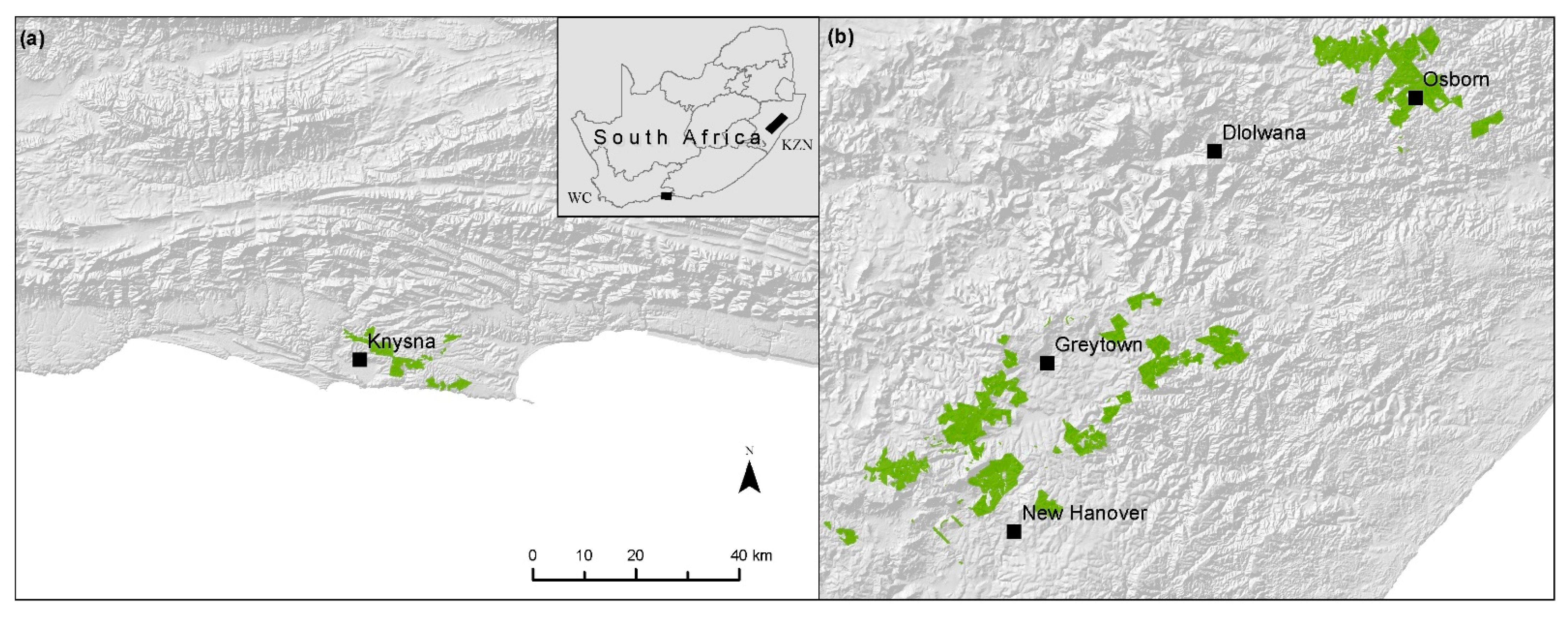
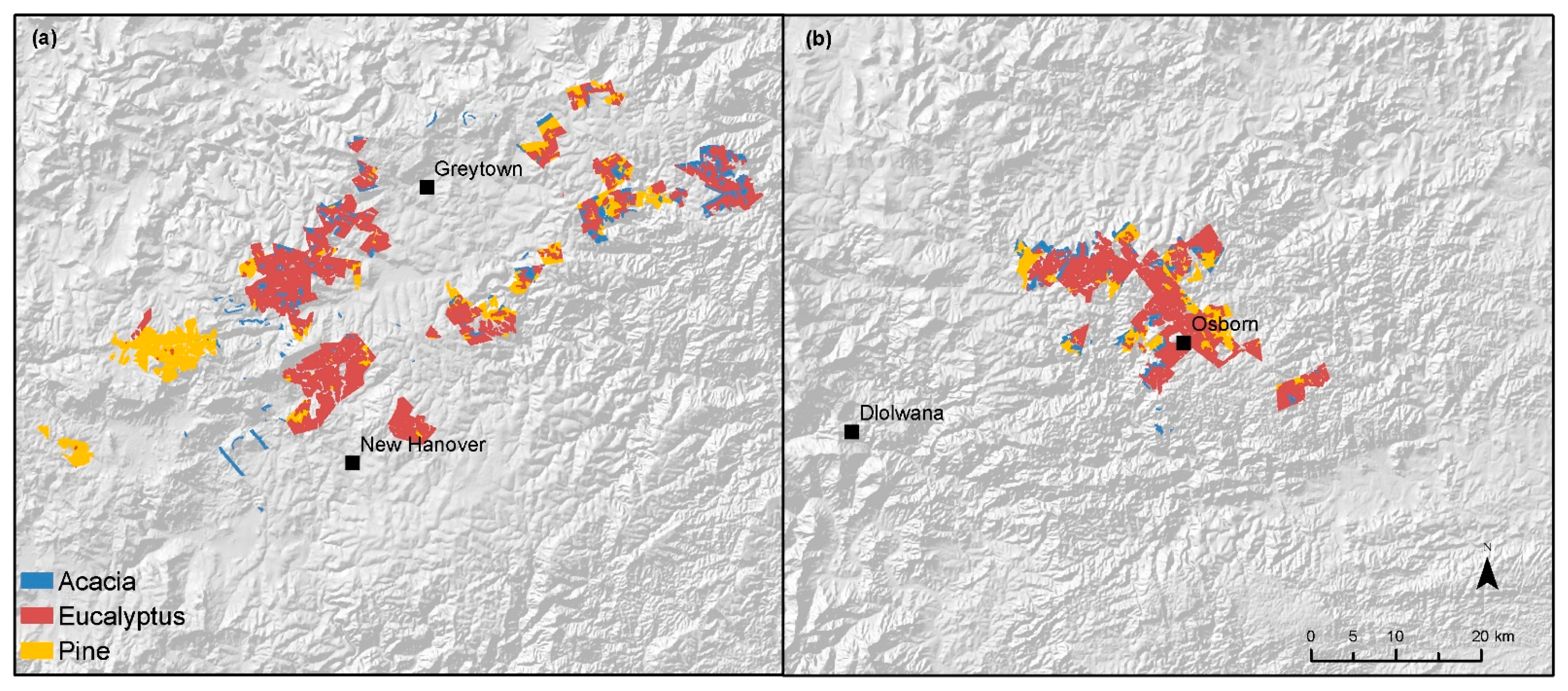
2.1. Study Areas

Two study sites (Figure 2) were selected for carrying out the experiments. Study Area 1 (23,117,207; −34,028,904) stretches from the settlements Knysna to Kraanshoek in the Western Cape (WC) province of South Africa, while Study Area 2 (30,939,643; −29,027,329) spans the settlements New Hanover to Osborn in KwaZulu-Natal (KZN). These sites were chosen owing to the diversity of the genera planted and the availability of reference data (i.e., in situ forest plantation extents and genera). The selected sites are also climatically representative, as they are located in the winter and summer rainfall regions of South Africa, respectively.

Study Area 1 receives ~875 mm of rainfall per annum, with peak rainfall during July. The mean temperature in the area is 16.9 °C [50]. The annual rainfall in Study Area 2 ranges from 1400 mm in the southwest to 1570 mm in the northeast (peak rainfall during January), and has a mean temperature of 17.5 °C [52].

Study Area 1 is dominated by Pinus (~3052 ha), followed by Eucalyptus (~145 ha) and then Acacia (~118 ha), whereas Study Area 2 is planted equally with Acacia (~3869 ha), Eucalyptus (~3869 ha), and Pinus (~3869 ha).

2.2. Data Collection and Preparation

2.2.1. Imagery

The GEE platform was used to access Sentinel-2 level-2A surface reflectance imagery, which has a five-day temporal resolution and contains 13 spectral bands, with spatial resolutions of 10 m (B2, B3, B4, and B8), 20 m (B5, B6, B7, B8A, B11, and B12), and 60 m (B1, B9, and B10). A median composite image was generated from images dated from 30 June 2019 to 30 June 2020. The reasoning behind using a composite image was to remove cloud contamination and to compensate for seasonal variations between the two study areas. Although it is well known that phenological variations and multi-temporal EO approaches can aid in genus classifications [33], we purposefully excluded such variations, as they would introduce uncertainty to our results. For instance, some training sample sets may benefit more from seasonal variations than others, which would add complexity and potentially skew the findings.

The normalized differential vegetation index (NDVI), enhanced vegetation index (EVI), entropy, and grey level co-occurrence matrix (GLCM) measures were derived from the NIR Sentinel-2 band and added as bands to the composite image, resulting in a total of 33 features (

Table 2. Features (bands, indices, and textural measures) used as inputs to the classifications generated from a composite of individual Sentinel-2 images taken from 30 June 2019 to 30 June 2020.

Bands	Textural Measures
B1—coastal aerosol	Angular second moment	Maximum correlation coefficient
B2—blue	Contrast	Cluster prominence
B3—green	Correlation	Sum average
B4—red	Difference entropy	Sum entropy
B5, B6, B7, B8A—vegetation red edge	Entropy	Cluster shade
B8—NIR	Inverse difference moment	Sum variance
B9—water vapour	Information measure of correlation 1	Variance
B10—SWIR—cirrus	Information measure of correlation 2
B11, B12—SWIR	Inertia
Vegetation Indices
NDVI
EVI

).

2.2.2. In Situ Data

In situ (ground-truth) data at the plantation compartment level were collated from a number of South African commercial forestry companies. These data included records of the species and genera of the trees in each compartment.

Table 3. Summary of in situ data (forest compartment information) collated, including tree genus, age (mean and standard deviation), and planted area per study area.

	Study Area 1 (WC)					Study Area 2 (KZN)
Genus	Age (Mean)	Age (Std Dev)	Area (ha)	Area (%)	#	Age (Mean)	Age (Std Dev)	Area (ha)	Area (%)	#
Acacia	35.94	12.61	118.14	3.56	40	8.75	7.10	3869.7	33.33	406
Eucalyptus	43.18	20.49	145.79	4.40	50	6.52	4.57	3869.4	33.33	718
Pinus	9.97	11.08	3052.81	92.04	940	8.78	6.50	3869.3	33.33	478
Total			3316.74		1030			11,608.4		1602

provides an overview of the collected in situ sample data per genus within each study area.

Figure 3 and Figure 4 show the geographic distribution of training data within Study Area 1 and Study Area 2, respectively. Compared to Study Area 1, the samples in Study Area 2 span a larger area and are more widely distributed. The areas covered by each genus in Study Area 1 are unbalanced (dominated by Pinus), while in Study Area 2 the area covered by each genus is more or less equal.

2.3. Experimental Design

The in situ data were consolidated into a shapefile and the compartments were dissolved to form a single polygon per genus. In total, 3000 random points were generated per genus (i.e., 9000 in total) in each study area. A maximum of one point per Sentinel-2 pixel was allowed. The polygons from which the training data were collected contained many compartments of different tree ages, and some with different species of the same genus. The variety of age and species per genus, along with the distance between samples produced by the randomness of the sample selection, minimized the autocorrelation in the training data. The Sentinel-2 band values were then extracted at each point in SS_0 using GEE. This initial sample sets were denoted P-3000, E-3000, and A-3000, representing Pinus, Eucalyptus, and Acacia species, respectively (with the first letter indicating the genus and the number indicating the subset size). This initial sample set was randomly subsampled into 60 subsets of decreasing sizes, starting from the full set and randomly removing 50 samples per iteration. For instance, the first Pinus subset (P-2950) contained 2950 samples, the second (P-2900) contained 2900 samples, the third (P-2850) contained 2850 samples, etc. A total of 180 sample sets (60 per genus) was generated in this manner.

The experiments (Figure 5) were designed to investigate the combined effect of training set size and imbalance on the RF classifier.

The aim of Experiment A was to quantify the effect of a balanced training sample set under different sample size scenarios. The experiment started (iteration 1) with using subsets P-3000, E-3000, and A-3000 to train the RF classifier. This model building process was repeated for combinations of subsets of equal sizes, e.g., for Experiment A, the following setup was used:

• Experiment A1: P-3000, E-3000, and A-3000
• Experiment A2: P-2950, E-2950, and A-2950
• …
• Experiment A60: P-50, E-50, and A-50

Experiments B1, B2, and B3 were similar to Experiment A, except that for all iterations the smallest subset (either P-50, E-50, or A-50) was used for one of the genera. For instance, the setup for Experiment B1 was as follows:

• Experiment B1.1: P-3000, E-3000, and A-50
• Experiment B1.2: P-2950, E-2950, and A-50
• …
• Experiment B1.3 60: P-50, E-50, and A-50

Similarly, E-50 was used in all iterations of Experiment B2:

• Experiment B2.1: P-3000, E-50, and A-3000
• Experiment B2.2: P-2950, E-50, and A-2950
• …
• Experiment B2.60: P-50, E-50, and A-50

In Experiment B3, P-50 was reused in all iterations:

• Experiment B2.1: P-50, E-3000, and A-3000
• Experiment B2.2: P-50, E-2950, and A-2950
• …
• Experiment B2.60: P-50, E-50, and A-50

Experiments B1 to B3 were conducted to assess the effect when one class (genus) is severely undersampled.

Experiments C1, C2, and C3 were similar to Experiments B1, B2, and B3, except that in all iterations the smallest subset was reused for two of the genera. For instance, in Experiment C1 the setup was as follows:

• Experiment C1.1: P-3000, E-50, and A-50
• Experiment C1.2: P-2950, E-50, and A-50
• …
• Experiment C1.60: P-50, E-50, and A-50

Similarly, for Experiment C2, the following setup was used:

• Experiment C2.1: P-50, E-3000, and A-50
• Experiment C2.2: P-50, E-2950, and A-50
• …
• Experiment C2.60: P-50, E-50, and A-50

The sample subsets for Experiment C3 were as follows:

• Experiment C3.1: P-50, E-50, and A-3000
• Experiment C3: P-50, E-50, and A-2950
• …
• Experiment C3.60: P-50, E-50, and A-50

Experiments C1 to C3 were designed to assess the effect when two classes (genera) are severely undersampled.

The purpose of the final experiment, Experiment D, was to assess the effects of area-proportional training datasets on classification accuracy. In contrast to the other experiments, Experiment D did not start with the full sample set. Instead, subsample sets were selected based on the relative area planted with a particular genus. Study Area 1 (WC) is dominated (92%) by Pinus compartments, while Eucalyptus (4.4%) and Acacia (3.6%) are not commonly planted. Consequently, the setup for Experiment D was as follows:

• Experiment D1: P-3000, E-240, and A-180
• Experiment D2: P-2950, E-236, and A-177
• …
• Experiment D60: P-50, E-4, and A-3

Experiment D was not implemented for Study Area 2 (KZN), given that the planted areas per genus are more or less equal, which equates to Experiment A.

2.4. Classifier Setup

RF, developed by Breiman [53], is an ensemble classifier, as it combines the results of multiple DT models. It uses 2/3 of the sample data, known as subset R1, for training the model. The remaining 1/3 of the samples, known as the out-of-bag (OOB) sample subset, are used to estimate the variable importance and the classification error. At each node within each DT, the algorithm selects a random subset of input features (bands), known as F1. It then uses subset R1 to identify the feature in F1 that best splits the data for a class and creates new nodes. This process is repeated at each node. Once all nodes are split for each tree, the majority vote among trees decides the final classification output [54]. All experiments were run using the default parameters of the RF algorithm to fairly compare the experiments. Each iteration (i.e., sample size change) was repeated 100 times, and the mean accuracy over all iterations was calculated to mitigate the stochastic nature of the RF algorithm.

2.5. Accuracy Assessment

An independent test sample set of 100 points per genus was used to calculate the overall accuracy (OA), kappa statistic (KS), consumer’s accuracy (CA), producer’s accuracy (PA), indices of disagreement [55], and McNemar’s test. The OA measures the percentage of pixels that are correctly classified, while the kappa statistic measures the chance of agreement between the reference and classified maps. The PA and CA are used to quantify the performance of each class. The PA shows the occurrence of features on the ground that are correctly shown on the classified map. The error of omission (EoO) can be calculated by 1-PA. The CA shows the occurrence of the class on the map that will actually be present on the ground. The error of commission can be calculated by 1-CA [56].

The RF algorithm was run 100 times per iteration (i.e., an experiment with a specific set of training data) to mitigate its stochastic nature (e.g., the accuracy of subsequent runs may differ substantially based on the internal random selection of the model for building samples and feature sets), and the mean OA, KS, CA, and PA were calculated from confusion matrices. The standard deviations of the 100 iterations of the OA and KS were also calculated to assess to what extent the calculated means were representative of the 100 iterations [57].

Indices of disagreement were analysed to validate the statistics derived from the confusion matrix, and McNemar’s test was used to analyse whether the differences between the OAs were statistically significant. To reduce computational expense, indices of disagreement and McNemar’s statistical test were calculated for only 7 of the 60 models, namely, Experiments A60, A50, A40, A30, A20, A10, and A1.

2.6. Spectral Analysis

The reflectance values of the samples (SS_0) were used to develop a spectral profile of each genus within each study area to assist with the interpretation of the results. A pairwise Jeffries–Matusita (J–M) distance separability analysis was carried out to better understand the interclass variations. The J–M distance quantifies the average distance between two classes in feature space based on a density function (i.e., probability distribution) of each class [58]. Both the mean and the variance are considered in the distance calculations. The J–M distances range from 0 to 2, where 0 represents a low separability between classes and 2 represents a high separability between classes.

3. Results

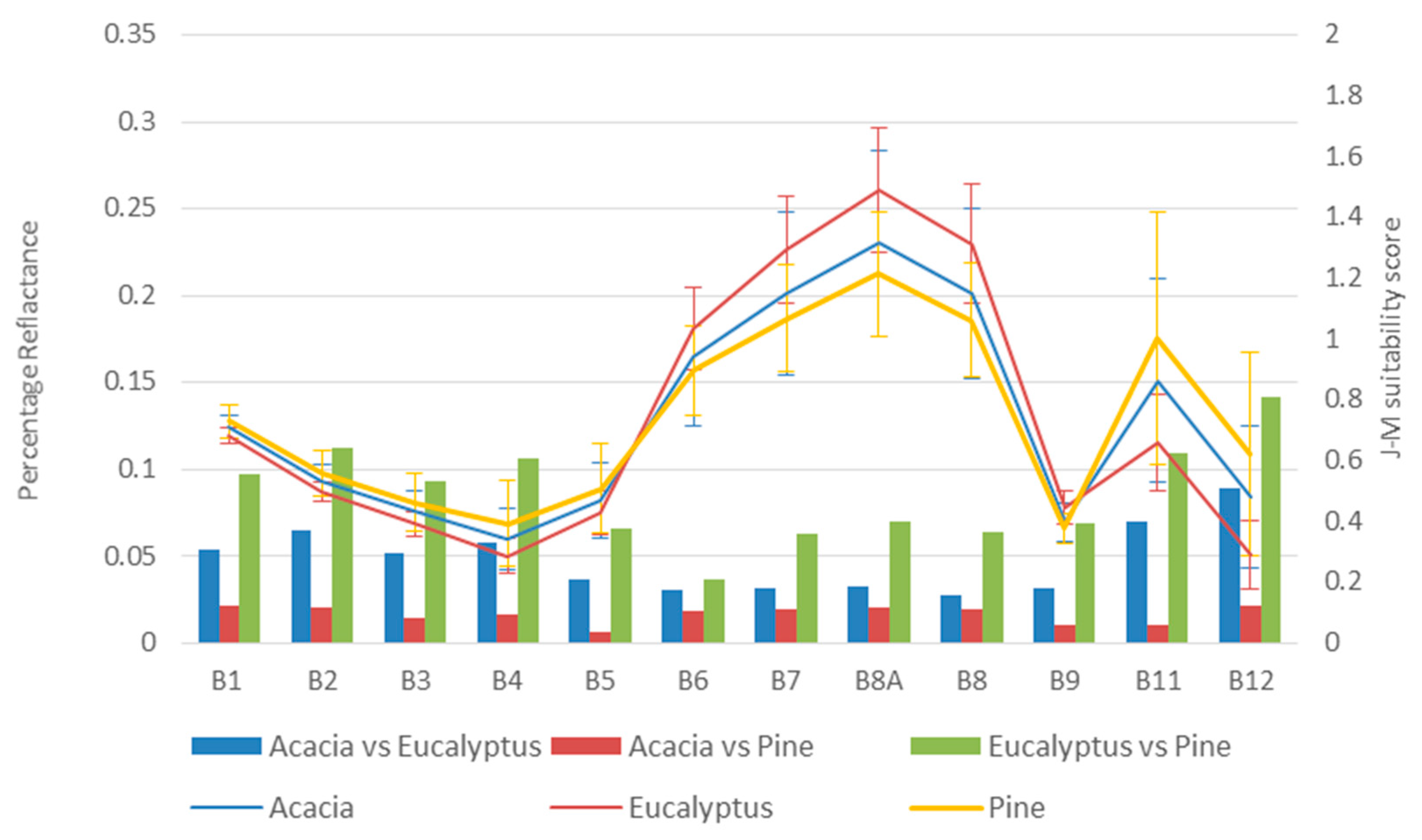
3.1. Genus Spectral Profiles

The spectral properties of the genera, as extracted from the S2 imagery and all SS_0 samples, are shown in Figure 6 for Study Area 1 and Figure 7 for Study Area 2. The spectral properties of trees are dependent on many factors, including age, specie composition, and location. The spectral signatures of the Acacia and Pinus classes were very similar, especially in Study Area 2 (KZN). Although it seemed that there were some differences in the mean values in bands B4, B6 to B8, and B11 to B12, there was a large spectral overlap between the classes (indicated by the error bars), suggesting that the genera are spectrally similar. This was confirmed by the J–M distance scores for the spectral bands (shown as bars in Figure 6 and Figure 7), where Eucalyptus and Pinus were the most separable, followed by Acacia and Eucalyptus, and to a lesser degree Acacia and Pinus. The highest separability (0.8) in Study Area 1 (WC) was between Eucalyptus and Pinus in B12 (Figure 6). These two genera were consistently the most separable in this region, which corresponds well with the spectral profiles (i.e., the mean reflectance values of Eucalyptus and Pinus are most distinct in almost all bands).

In Study Area 1 (WC), the visible (B2, B3, and B4) and SWIR (B11 and B12) regions of the EMS had a higher separability (0.4–0.7) than the red-edge region (0–0.3) of the EMS (Figure 6). The SWIR wavelengths are known to be absorbed by vegetation with high moisture content [59]. This suggests that the water content varies between the plantation genera in Study Area 1.

In contrast, all three genera in Study Area 2 (KZN) had low separability in the visible and SWIR regions of the EMS, suggesting that the genera have similar water contents (Figure 7). The strongest separability scores (0–0.33) were recorded in the red-edge (B6 and B7), near-infrared (B8 and B8A), and water vapour (B9) bands (Figure 7). Eucalyptus and Pinus trees were the most separable, followed by Acacia and Eucalyptus.

When the spectral profiles are compared, it is clear that Pinus and Acacia trees have very similar spectral responses, while those of Eucalyptus trees are more distinct.

Table 4. Jefferies–Matusita difference scores between Acacia and Eucalyptus, Acacia and Pinus, and Eucalyptus and Pinus using Sentinel-2 bands; Sentinel-2 bands and vegetation indices; and Sentinel-2 bands, vegetation indices, and textural features for both study areas.

	Acacia vs. Eucalyptus		Acacia vs. Pinus		Eucalyptus vs. Pinus
	WC	KZN	WC	KZN	WC	KZ N
Sentinel-2 bands	0.01615204	0.027278119	0.01083795	0.001678353	0.0427256	0.041993623
Sentinel-2 bands and vegetation indices	0.02963264	0.017471886	0.01521441	0.002094672	0.08139061	0.031343328
Sentinel-2 bands, vegetation indices, and textural features	0.1258648	0.2534354	0.2615191	0.0000066	0.578058	0.2554823

shows the total J–M separability scores using just the Sentinel-2 bands; the Sentinel-2 bands and vegetation indices; and the Sentinel-2 bands, vegetation indices, and textural measures, which also suggests that Eucalyptus trees are more dissimilar than Pinus and Acacia trees.

Table 4 shows that adding vegetation indices and textural features to the Sentinel-2 bands increased the separability between all classes in Study Area 1 (WC). This suggests that the machine learning algorithms produce better results using Sentinel-2 bands along with vegetation indices and textural features as inputs. The separability scores in Study Area 2 (KZN) varied between band combinations and between classes. The addition of vegetation indices only increased the separability between Acacia and Pinus. The separability between Eucalyptus and Pinus, and between Acacia and Eucalyptus, increased when textural features were included, but decreased when vegetation indices were included.

3.2. Classification

Table S1, in the Supplementary Materials, summarizes the classification results. To aid in the interpretation, important results are shown in bold text; high accuracies are shown green and lower accuracies in red, while high standard deviations are shown in red and low standard deviations in blue. When compared to the number of features (n), this initial subset’s size (s) can be expressed as s~91n (i.e., about two samples per feature/dimension, per genus). From Experiment A, it is evident that larger training sample set sizes (s > n) resulted in higher OAs. In Study Area 1 (WC), the highest mean OA (76.3%) and best individual classification result (Max OA = 81.3%) were achieved when all (100%) of the available samples (SS_0) were used for training. However, the improvement in accuracy was not linear (Figure S1: A1), with the OA increasing by only 2% when the sample size was enlarged from 67% (s~60n) to 100% (s~90n), which is insignificant given that the standard deviation is about 0.02% for these experiments. The same trend can be observed in Study Area 2 (KZN) (Figure S1: A4), although fewer (50%) training samples were required for achieving the maximum OA (70.7%). The mean OA of all experiments in Study Area 1 (79.8%) was significantly (p > 0.001, shown in Table S2) higher than that of Study Area 2 (76.7%).

When the PAs and CAs are considered in Study Area 1 (WC) (Figure S1: A2 and A3), it is clear that the Eucalyptus class was the most accurately classified, as it had the lowest errors of omission and commission, followed by Pinus and then Acacia. In Study Area 2 (KZN), the PAs and CAs of the three genera were relatively similar.

The experiments dealing with imbalanced training sets (Experiments B–D) showed that the OAs and KSs remain relatively constant as sample imbalance increases. The CAs of the class for which the training subset with 50 samples (either P-50, E-50, or A-50) was used in all iterations were generally higher (Figure S1: B2, B5, C2, C5, D2, D5) than those of the two classes for which the training subsets were systematically enlarged, indicating that the errors of commission (i.e., false positives) were relatively low for this class. Conversely, the PAs (Figure S1: B3, B6, C3, C6, D3, D6) of the genus for which the smallest training set (either P-50, E-50, or A-50) was used were consistently lower compared to those of the other two genera.

In Experiments C1–C3 (where a pair of P-50, E-50, or A-50 were used in all iterations), the OA and KS decreased as the sample imbalance increased. The CA of the class for which the sample size was systematically enlarged was generally lower (Figure S1: C1.2, C1.5, C2.2, C2.5, C3.2, C3.5) than that of the two classes for which the training subset was kept constant at 50 samples throughout all iterations. Conversely, the PA (Figure S1: C1.3, C1.6, C2.3, C2.6, C3.3, C3.6) of the genus for which the training set was enlarged was consistently higher compared to the other two genera for which the training sets were kept constant at 50 samples.

In Experiment D, Study Area 2 (KZN) had consistently higher OAs and KSs than Study Area 1 (WC). The OAs and KSs for Study Area 1 (Figure S1: D1) were relatively low and stable when the sample size was enlarged in proportion to the area being mapped. Eucalyptus had the highest CA, followed by Acacia and then Pinus (Figure S1: D2). The PA of Pinus was the highest, followed by Eucalyptus and then Acacia (Figure S1: D3). Conversely, the increases in OAs and KSs for Study Area 2 (Figure S1: D4) were initially dramatic, but then moderated to within the 95% confidence level of ~0.05 as the sample size was enlarged. Additionally, the CAs and PAs among classes were relatively similar in this study area (Figure S1: D5, D6).

In summary, the results show that the highest accuracy was achieved when an equal number of training samples per class was used (mean OA of 72.2% for Experiment A). The OAs generally increased as the training sample sets were enlarged, but only when the training datasets were balanced. Comparatively low classification accuracy was achieved when unbalanced training samples were used. A trend of low errors of commission (i.e., false positives) and high errors of omission (false negatives) was noted for under-represented classes (i.e., those for which the sample sizes were not systematically enlarged). The classification accuracy was generally higher (mean OA of 61.8%) in Study Area 2, where the areas covered by the sampled genera were similar in proportions, while the accuracy was generally low (mean OA of 53%) when an area-proportional sampling strategy was used to differentiate the genera in Study Area 1, i.e., where the targeted area of interest (i.e., the population from which sampling was done) was dominated by one class (Pinus).

4. Discussion

Satellite remote sensing, combined with machine learning, has been shown to be effective for monitoring plantation forests [17] and for differentiating forest plantation genera/species [33]. However, machine learning requires labelled (in situ) data for model training and validation. The cost of collecting large quantities of such data can impede regional implementations. Given that classification accuracy is strongly related to the size of training datasets [45], operational solutions should ideally strike a balance between classification accuracy and training data collection efforts. However, very little is known about how training set size impacts forest plantation genus classification accuracy. It is also not clear whether the number of samples per class should be proportional to the targeted populations—as suggested by Colditz [49], Millard and Richardson [47], and Shetty [60]—or if an equal number of samples per class would be most effective, as suggested by Mellor et al. [48] and Thanh Noi and Kappas [43]. A further complication is that the distributions and proportions of genera vary greatly from region to region—often with one or two dominating genera—meaning that sampling strategies might have to be region-dependent.

In this study, we investigated the effects of different sampling strategies on the performance of the RF machine learning classifier for differentiating between three genera in two diverse regions, using 33 features extracted from a cloud-free Sentinel-2 composite image as inputs. Our findings are consistent with those of Myburgh and Van Niekerk [61], who showed that higher (~90%) classification accuracy was achieved when the number of samples per class was increased from s~0.5n to s~2n, but that the relationship between the number of samples per class and accuracy was nonlinear. This was attributed to the reduction in sparsity as samples were added until the training samples sufficiently represented inter- and intraclass spectral variations. Similarly, Heydari and Mountrakis [62] found that classification accuracy increased by 2–6% when the training sample size was enlarged from s~37n to s~370n respectively, but the accuracy tended to flatten out at s = 2218 (s~370n). Enlarging the training set beyond this saturation point [45] did not add any value to the classification. Based on our data (Experiment A), a saturation point was reached at s~2100 (s~64n) when the samples per class were balanced. This suggests that collecting more than 64n training samples per class may be superfluous for our particular application.

Our results show that the RF classifier did not handle the unbalanced training datasets well. Generally, low error of commission (i.e., false positives) and high error of omission (i.e., false negatives) were noted for minority (under-represented) classes (i.e., those for which the sample sizes were not systematically enlarged). Pixels belonging to the majority class were often erroneously allocated to the minority class. This is consistent with the work of Mellor et al. [48], who found that majority classes performed well at the expense of minority classes when the training sets were unbalanced. The RF classifier is an ensemble of tree classifiers, where each tree makes its decision based on a set of rules derived from labelled features (i.e., training data) [63], and a majority vote is used to determine the consensus class [64]. Classes with larger training datasets tend to have fewer false negatives (i.e., omission errors), as a larger set of rules (i.e., splitters) can be constructed. In contrast, classes with limited training data are likely to have fewer false positives (i.e., errors of commission), as insufficient data are available for constructing splitting rules.

It is clear from our results that spectral separability among classes also played a role in classification accuracy, with low-separability classes generally requiring a larger proportion of samples compared to those with high separability [48]. In our application, the spectral properties of Eucalyptus trees were the most distinct, resulting in larger differences in CAs between classes when the sample size of Eucalyptus was contained (C2 compared to B2 and D2 in Figure S1). For Study Area 1 (WC), the separability between classes improved when vegetation indices and textural measures were included as inputs to the classifier. This is to be expected, as vegetation indices are known to help differentiate between variations in vegetation vigour and biomass [37]. Textural measures show the patterns amongst pixels, which are not represented in the spectral properties of each pixel [35]. However, the separability results in Study Area 2 (KZN) showed that vegetation indices did not improve the discrimination of classes. This was attributed to this area containing a larger proportion of recently planted compartments, where the ratio between bare ground and vegetation was larger and, thus, reduced the efficiency of the vegetation indices [36].

Colditz [49] and Shetty [60] evaluated the effects of different sampling designs on ML classifications for land cover, and found that area-proportional samples resulted in the best accuracy. This is consistent with the findings Millard and Richardson [47], who recommended randomly selected, area-proportional training sets. In contrast to these findings, an area-proportional sampling scheme performed poorly in our Study Area 1 (Experiment D). Study Area 1 is dominated by Pinus (ratios of Acacia, Eucalyptus, and Pinus are about 1:1:26), which resulted in highly skewed training sets in Experiment D. According to Figure S1 D2 and D3, the Pinus class was overclassified (i.e., low CA, high error of commission), while the Acacia and Eucalyptus classes were underclassified (i.e., low PA, high error of omission). For example, the error of omission (EoO = 1 − PA) of the Acacia class exceeded 86% throughout the experiment, even when s~3n for this class. In contrast, in Experiment A (balanced samples), the error of omission for Acacia was 37% when s~2n (initialization of Experiment A). This suggests that an area-proportional sampling approach is not effective when the populations (i.e., total number of pixels) of some classes are severely skewed (i.e., where some classes dominate, while others are under-represented). Based on our data, it seems that an area-proportional approach to training sample selection is beneficial only if some classes are not severely under-represented. Based on Experiments B–D, when three classes are targeted and one class is under-represented, the ratio of the under-represented class should never be less than 1:50:50. When two classes are under-represented (or one class dominates), this ratio should preferably not exceed 1:1:50. However, whether these suggested ratios are applicable for other applications would have to be investigated in future research. Based on our data, a balanced training set (Experiment A) produced the most consistent (stable) per-class (i.e., PAs and CAs) results for both the skewed (Study Area 1) and equivalent (Study Area 2) populations. This is consistent with the findings of Foody and Mathur [45], Mellor et al. [48], and Thanh Noi and Kappas [43]. A balanced training set is consequently recommended for operational forest plantation genus mapping in South Africa. Apart from producing the best results in this study, it is simple to implement, and do not require prior knowledge of the distribution of classes.

Our results show that OA was often not a good reflection of overall class performance, particularly when training data were unbalanced. For instance, it is noticeable that the mean OA of Experiment D in Study Area 1 was 64%, while it is clear that Pinus had a low mean PA (29%) and Acacia had a low CA (55%). This demonstrates that OA is an unreliable measure of accuracy, particularly when the training data are skewed. In contrast to a previous work by Pontius and Millones [55], the mean KS of Experiment D in Study Area 1 was low (0.45), better depicting the overall performance of the experiment. Similarly, the OAs of Experiments B–C were relatively high, while they resulted in varying CAs and PAs. The relatively low KSs of these experiments are consequently better indicators of the overall classification performance, and they corresponded to indices of disagreement (see the Supplementary Materials). This is consistent with the findings of Viera and Garrett [65] and Thanh Noi and Kappas [43], who observed that OA was often misleading when the training datasets were unbalanced. We recommend that in future studies OA should be supplemented by other accuracy metrics, such as kappa and disagreement—especially if unbalanced datasets are being classified.

Although the purpose of this study was not to assess the efficacy of machine learning for genus classification, our findings show that accuracy exceeding 80% can be achieved when a composite S2 image (and its derivatives) is used as an input. Better results are likely when the methodology is extended to incorporate multi-temporal imagery, data fusion (e.g., the combination of SAR data), feature selection/extraction, and alternative machine learning techniques (e.g., ANNs, SVMs). Operationalizing such approaches will enable more frequent national forest inventorying at a reduced cost compared to traditional (field survey) methods. However, this study shows that training sample design significantly affects classification results, and that it is critical that data collection efforts be carried out accordingly.

Although this study demonstrates potential for classifying the main forest plantation genera in two very diverse study areas (WC and KZN) with very different rainfall and temperature regimes, more work is needed to evaluate the transferability of machine learning models to other regions. Our results show that the sample set should be ~64n within each area being mapped, but we did not assess whether samples could be extended to classify genera in other regions where no samples are available. Signature extension and model transferability should be investigated in future works, as this could reduce the costs of in situ training data collection.

Another limitation of this study is that the classifications were performed on known plantation forest compartments (polygons). In reality, such data are often not available for regional applications. Although plantation forests are usually included in national land-cover maps (e.g., SANLC), a methodology whereby plantation forests can be separated from other land-cover types and classified into genera would be of great value for operational implementations.

5. Conclusions

Although it is known that the accuracy of machine learning approaches for classifying remotely sensed imagery is affected by training data size and configuration, little is known about how different sampling strategies may affect the differentiation of forest plantation genera. This study evaluated the effects of several training dataset configurations on RF’s ability to classify Acacia, Eucalyptus, and Pinus trees in two diverse regions within South Africa. The RF algorithm was implemented using bands, spectral indices, and textural measures extracted from a Sentinel-2 composite image as input features (n = 33). In situ forest plantation data were used to generate various sample sets, which were used to train and assess the ability of the RF classifier to differentiate between genera.

Our findings show that although the spectral separability of classes affected the ability of RF to accurately differentiate between forest plantation genera, the classification accuracy was mainly influenced by training sample size and imbalance. Balanced training datasets produced the most accurate and consistent results, while unbalanced training data did not work well for differentiating genera using RF. It is clear that sampling scheme design is critical for regional forest genus mapping implementations, and that a balanced approach is needed for in situ (labelled) data collection efforts. Although the purpose of this study was not to assess the value of Sentinel-2 imagery for genus classifications, our results suggest that such imagery, combined with machine learning, holds much potential for this purpose. Future research should consider a multi-temporal approach to exploit the phenological differences between genera. Model transferability and/or sample extension should also be investigated to minimize sample collection efforts. Answering these questions may lead to operational solutions for mapping forest plantation genera at regional/national scales, and for regularly updating forest inventories. Accurate and up-to-date inventories will allow for improved land and forest management, water-use assessments, carbon stock estimates, and streamflow reduction modelling.

References

1. Xulu, S.; Peerbhay, K.Y.; Forests, S.; Gebreslasie, M. Remote sensing of forest health and vitality: A South African perspective. South. For. 2018, 1, 12. [Google Scholar] [CrossRef]
2. Poynton, R.J. A Silviculturalmap of Southern Africa. S. Afr. J. Sci. 1971, 67, 58–60. [Google Scholar]
3. FP&M SETA. Paper and Pulp Sector; FP&M SETA: Johannesburg, South Africa, 2014. [Google Scholar]
4. Steyl, I. Strategic Environmental Assessment for Stream Flow Reduction Activities in South Africa; Department of Water Affairs & Forestry, South Africa: Pretoria, South Africa, 1997; pp. 1–14. [Google Scholar]
5. Wicks, T.E.; Smith, G.M.; Curran, P.J. Polygon-based aggregation of remotely sensed data for regional ecological analyses. Int. J. Appl. Earth Obs. Geoinf. 2002, 4, 161–173. [Google Scholar] [CrossRef]
6. Scott, D.F.; Prinsloo, F.W.; Moses, G.; Mehlomakulu, M.; Simmers, A.D.A. A Re-Analysis of the South African Catchment Afforestation Experimental Data: Report to the Water Research Commission; WRC: Pretoria, South Africa, 2000. [Google Scholar]
7. Savage, M.J.; Odhiambo, G.O.; Mengistu, M.G.; Everson, C.S.; Jarmain, C. Measurement of grassland evaporation using a surface-layer scintillometer. Water SA 2010, 36, 1–8. [Google Scholar] [CrossRef]
8. van Wyk, D.B. Some Effects of Afforestation on Streamflow in the Western Cape Province, South Africa. Water SA 1987, 12, 31–36. [Google Scholar]
9. Van Der Zel, D.W. Accomplishments and Dynamics of the South African Afforestation Permit System. South Afr. For. J. 1995, 172, 49–58. [Google Scholar] [CrossRef]
10. Gush, M.B.; Scott, D.F.; Jewitt, G.P.W.; Schulze, R.E.; Hallowes, L.A.; Görgens, A.H.M. A new approach to modelling streamflow reductions resulting from commercial afforestation in south africa. S. Afr. For. J. 2002, 196, 27–36. [Google Scholar] [CrossRef]
11. Clulow, A.D.; Everson, C.S.; Gush, M.B. The Long-Term Impact of Acacia Mearnsii Trees on Evaporation, Streamflow and Groundwater Resources; Water Research Commission Report No. TT505/11; WRC: Pretoria, South Africa, 2011. [Google Scholar]
12. FSA. Environmental Guidelines for Commercial Forestry Plantations in South Africa; Forestry South Africa: Johannesburg, South Africa, 2019; pp. 1–130. [Google Scholar]
13. Forestry South Africa. Timber Plantation Ownership; Forestry South Africa: Johannesburg, South Africa, 2019. [Google Scholar]
14. Schulz, J.; Albert, P.; Behr, H.D.; Caprion, D.; Deneke, H.; Dewitte, S.; Dürr, B.; Fuchs, P.; Gratzki, A.; Hechler, P.; et al. Operational climate monitoring from space: The EUMETSAT satellite application facility on climate monitoring (CM-SAF). Atmos. Chem. Phys. 2009, 9, 1687–1709. [Google Scholar] [CrossRef]
15. Jokar Arsanjani, J.; Tayyebi, A.; Vaz, E. GlobeLand30 as an alternative fine-scale global land cover map: Challenges, possibilities, and implications for developing countries. Habitat Int. 2016, 55, 25–31. [Google Scholar] [CrossRef]
16. Department of Environmental Affairs. South African National Land-Cover 2018 Report & Accuracy Assessment; Department of Environmental Affairs, South Africa: Pretoria, South Africa, 2019; Volume 4. [Google Scholar]
17. Lück, W. Generating Automated Forestry Geoinformation Products From Remotely Sensed Imagery. Master’s Thesis, Stellenbosch Unviersity, Stellenbosch, South Africa, 2018. [Google Scholar]
18. Franco-Lopez, H.; Ek, A.R.; Bauer, M.E. Estimation and mapping of forest stand density, volume, and cover type using the k-nearest neighbors method. Remote Sens. Environ. 2001, 77, 251–274. [Google Scholar] [CrossRef]
19. Stabach, J.A.; Dabek, L.; Jensen, R.; Wang, Y.Q. Discrimination of dominant forest types for Matschie’s tree kangaroo conservation in Papua New Guinea using high-resolution remote sensing data. Int. J. Remote Sens. 2009, 30, 405–422. [Google Scholar] [CrossRef]
20. Cho, M.A.; Malahlela, O.; Ramoelo, A. Assessing the utility WorldView-2 imagery for tree species mapping in South African subtropical humid forest and the conservation implications: Dukuduku forest patch as case study. Int. J. Appl. Earth Obs. Geoinf. 2015, 38, 349–357. [Google Scholar] [CrossRef]
21. Francois, A.; Leckie, D.G. Francios The individual tree crown approach to Ikonos images of a Coniferous Plantation Area. In Photogrammetric Engineering & Remote Sensing; American Society for Photogrammetry and Remote Sensing: Victoria, Canada, 2006. [Google Scholar]
22. Immitzer, M.; Atzberger, C.; Koukal, T. Tree species classification with Random forest using very high spatial resolution 8-band worldView-2 satellite data. Remote Sens. 2012, 4, 2661–2693. [Google Scholar] [CrossRef]
23. Ke, Y.; Quackenbush, L.J.; Im, J. Remote Sensing of Environment Synergistic use of QuickBird multispectral imagery and LIDAR data for object-based forest species classi fi cation. Remote Sens. Environ. 2010, 114, 1141–1154. [Google Scholar] [CrossRef]
24. Pu, R.; Landry, S. A comparative analysis of high spatial resolution IKONOS and WorldView-2 imagery for mapping urban tree species. Remote Sens. Environ. 2012, 124, 516–533. [Google Scholar] [CrossRef]
25. Franklin, S.E.; Ahmed, O.S.; Williams, G. Northern Conifer Forest Species Classification Using Multispectral Data Acquired from an Unmanned Aerial Vehicle. Photogramm. Eng. Remote Sens. 2017, 83, 501–507. [Google Scholar] [CrossRef]
26. Franklin, S.E.; Ahmed, O.S. Deciduous tree species classification using object-based analysis and machine learning with unmanned aerial vehicle multispectral data. Int. J. Remote Sens. 2018, 39, 5236–5245. [Google Scholar] [CrossRef]
27. Buddenbaum, H.; Schlerf, M.; Hill, J. Classification of coniferous tree species and age classes using hyperspectral data and geostatistical methods. Int. J. Remote Sens. 2005, 26, 5453–5465. [Google Scholar] [CrossRef]
28. Bujang, M.A.; Baharum, N. Guidelines of the minimum sample size requirements for Cohen’ s Kappa. Epidemiol. Biostat. Public Health 2017, 17, e12267. [Google Scholar]
29. Fagan, M.E.; DeFries, R.S.; Sesnie, S.E.; Arroyo-Mora, J.P.; Soto, C.; Singh, A.; Townsend, P.A.; Chazdon, R.L. Mapping species composition of forests and tree plantations in northeastern Costa Rica with an integration of hyperspectral and multitemporal landsat imagery. Remote Sens. 2015, 7, 5660–5696. [Google Scholar] [CrossRef]
30. Peerbhay, K.Y.; Mutanga, O.; Ismail, R. Commercial tree species discrimination using airborne AISA Eagle hyperspectral imagery and partial least squares discriminant analysis (PLS-DA) in KwaZulu-Natal, South Africa. ISPRS J. Photogramm. Remote Sens. 2013, 79, 19–28. [Google Scholar] [CrossRef]
31. Voss, M.; Sugumaran, R. Seasonal effect on tree species classification in an urban environment using hyperspectral data, LiDAR, and an object-oriented approach. Sensors 2008, 8, 3020–3036. [Google Scholar] [CrossRef] [PubMed]
32. Nomura, K.; Mitchard, E.T.A. More than meets the eye: Using Sentinel-2 to map small plantations in complex forest landscapes. Remote Sens. 2018, 10, 1693. [Google Scholar] [CrossRef]
33. Mngadi, M.; Odindi, J.; Peerbhay, K.; Mutanga, O. Examining the effectiveness of Sentinel-1 and 2 imagery for commercial forest species mapping. Geocarto Int. 2019, 36, 1–12. [Google Scholar] [CrossRef]
34. Vaglio Laurin, G.; Puletti, N.; Hawthorne, W.; Liesenberg, V.; Corona, P.; Papale, D.; Chen, Q.; Valentini, R. Discrimination of tropical forest types, dominant species, and mapping of functional guilds by hyperspectral and simulated multispectral Sentinel-2 data. Remote Sens. Environ. 2016, 176, 163–176. [Google Scholar] [CrossRef]
35. Feng, Q.; Liu, J.; Gong, J. Urban flood mapping based on unmanned aerial vehicle remote sensing and random forest classifier-A case of yuyao, China. Water 2015, 7, 1437–1455. [Google Scholar] [CrossRef]
36. Huete, A.; Didan, K.; Miura, T.; Rodriguez, E.P.; Gao, X.; Ferreira, L.G. Overview of the radiometric and biophysical performance of the MODIS vegetation indices. Remote Sens. Environ. 2002, 83, 195–213. [Google Scholar] [CrossRef]
37. Lukas, V.; Novák, J.; Neudert, L.; Svobodova, I.; Rodriguez-Moreno, F.; Edrees, M.; Kren, J. The combination of UAV survey and Landsat imagery for monitoring of crop vigor in precision agriculture. Int. Arch. Photogramm. Remote Sens. Spat. Inf. Sci. 2016, 41, 953–957. [Google Scholar] [CrossRef]
38. Loggenberg, K.; Strever, A.; Greyling, B.; Poona, N. Modelling water stress in a Shiraz vineyard using hyperspectral imaging and machine learning. Remote Sens. 2018, 10, 202. [Google Scholar] [CrossRef]
39. Ma, W.; Gong, C.; Hu, Y.; Meng, P.; Xu, F. The Hughes phenomenon in hyperspectral classification based on the ground spectrum of grasslands in the region around Qinghai Lake. In International Symposium on Photoelectronic Detection and Imaging 2013: Imaging Spectrometer Technologies and Applications; SPIE: Bellingham, DC, USA, 2013; Volume 8910, pp. 363–373. [Google Scholar]
40. Belgiu, M.; Dragut, L. Random forest in remote sensing: A review of applications and future directions. ISPRS J. Photogramm. Remote Sens. 2016, 114, 24–31. [Google Scholar] [CrossRef]
41. Congalton, R.G.; Green, K. Assessing the Accuracy of Remotely Sensed Data, 3rd ed.; Assessing the Accuracy of Remotely Sensed Data; Taylor & Francis Group: London, UK, 2019; pp. 87–106. [Google Scholar]
42. Mather, P.M. Computer Processing of Remotely-Sensed Images, 3rd ed.; John Wiley & Sons Ltd.: Hoboken, NJ, USA, 2004. [Google Scholar]
43. Thanh Noi, P.; Kappas, M. Comparison of Random Forest, k-Nearest Neighbor, and Support Vector Machine Classifiers for Land Cover Classification Using Sentinel-2 Imagery. Sensors 2017, 18, 18. [Google Scholar] [CrossRef] [PubMed]
44. Foody, G.M. Sample size determination for image classification accuracy assessment and comparison. Int. J. Remote Sens. 2009, 30, 5273–5291. [Google Scholar] [CrossRef]
45. Foody, G.M.; Mathur, A.; Sanchez-Hernandez, C.; Boyd, D.S. Training set size requirements for the classification of a specific class. Remote Sens. Environ. 2006, 104, 1–14. [Google Scholar] [CrossRef]
46. Dalponte, M.; Ørka, H.O.; Gobakken, T.; Gianelle, D.; Næsset, E. Tree species classification in boreal forests with hyperspectral data. IEEE Trans. Geosci. Remote Sens. 2013, 51, 2632–2645. [Google Scholar] [CrossRef]
47. Millard, K.; Richardson, M. On the importance of training data sample selection in Random Forest image classification: A case study in peatland ecosystem mapping. Remote Sens. 2015, 7, 8489–8515. [Google Scholar] [CrossRef]
48. Mellor, A.; Boukir, S.; Haywood, A.; Jones, S. Exploring issues of training data imbalance and mislabelling on random forest performance for large area land cover classification using the ensemble margin. ISPRS J. Photogramm. Remote Sens. 2015, 105, 155–168. [Google Scholar] [CrossRef]
49. Colditz, R.R. An evaluation of different training sample allocation schemes for discrete and continuous land cover classification using decision tree-based algorithms. Remote Sens. 2015, 7, 9655–9681. [Google Scholar] [CrossRef]
50. Kraaij, T.; Baard, J.A.; Arndt, J.; Vhengani, L.; van Wilgen, B.W. An assessment of climate, weather, and fuel factors influencing a large, destructive wildfire in the Knysna region. S. Afr. Fire Ecol. 2018, 14, 4. [Google Scholar] [CrossRef]
51. ESA. ESA’s Optical High-Resolution Mission for GMES Operational Services; ESA: Paris, France, 2015; 88p. [Google Scholar]
52. Fuller, J.A.; Perrin, M.R. Habitat assessment of small mammals in the Umvoti Vlei conservancy, KwaZulu-Natal, South Africa. Afr. J. Wildl. Res. 2001, 31, 1–12. [Google Scholar]
53. Breiman, L. Random forests. Mach Learn. 2001, 45, 5–32. [Google Scholar] [CrossRef]
54. Budei, B.C.; St-Onge, B.; Hopkinson, C.; Audet, F.A. Identifying the genus or species of individual trees using a three-wavelength airborne lidar system. Remote Sens. Environ. 2018, 204, 632–647. [Google Scholar] [CrossRef]
55. Pontius, R.G.; Millones, M. Death to Kappa: Birth of quantity disagreement and allocation disagreement for accuracy assessment. Int. J. Remote Sens. 2011, 32, 4407–4429. [Google Scholar] [CrossRef]
56. Foody, G.M. Status of land cover classification accuracy assessment. Remote Sens. Environ. 2002, 80, 185–201. [Google Scholar] [CrossRef]
57. Rodriguez-Galiano, V.F.; Ghimire, B.; Rogan, J.; Chica-Olmo, M.; Rigol-Sanchez, J.P. An assessment of the effectiveness of a random forest classifier for land-cover classification. ISPRS J. Photogramm. Remote Sens. 2012, 67, 93–104. [Google Scholar] [CrossRef]
58. Mahdianpari, M.; Salehi, B.; Mohammadimanesh, F.; Homayouni, S.; Gill, E. The first wetland inventory map of newfoundland at a spatial resolution of 10 m using sentinel-1 and sentinel-2 data on the Google Earth Engine cloud computing platform. Remote Sens. 2019, 11, 43. [Google Scholar] [CrossRef]
59. Manna, S.; Raychaudhuri, B. Mapping distribution of Sundarban mangroves using Sentinel-2 data and new spectral metric for detecting their health condition. Geocarto Int. 2020, 35, 434–452. [Google Scholar] [CrossRef]
60. Shetty, S. Analysis of Machine Learning Classifiers for LULC Classification on Google Earth Engine Analysis of Machine Learning Classifiers for LULC Classification on Google Earth Engine. Masters Thesis, University of Twente, Twente, The Nerthelands, 2019; pp. 1–65. [Google Scholar]
61. Myburgh, G.; Van Niekerk, A. Impact of training set size on object-based land cover classification: A comparison of three classifiers. Int. J. Appl. Geospatial. Res. 2014, 5, 49–67. [Google Scholar] [CrossRef]
62. Heydari, S.S.; Mountrakis, G. Effect of classifier selection, reference sample size, reference class distribution and scene heterogeneity in per-pixel classification accuracy using 26 Landsat sites. Remote Sens. Environ. 2018, 204, 648–658. [Google Scholar] [CrossRef]
63. Pal, M. Random forest classifier for remote sensing classification. Int. J. Remote Sens. 2005, 26, 217–222. [Google Scholar] [CrossRef]
64. Gislason, P.O.; Benediktsson, J.A.; Sveinsson, J.R. Random forests for land cover classification. Pattern Recognit. Lett. 2006, 27, 294–300. [Google Scholar] [CrossRef]
65. Viera, A.J.; Garrett, J.M. Understanding interobserver agreement: The kappa statistic. Fam. Med. 2005, 37, 360–363. Available online: http://www1.cs.columbia.edu/~julia/courses/CS6998/Interrater_agreement.Kappa_statistic.pdf (accessed on 4 April 2022). [PubMed]
Figure 1. Distribution of South African forest plantations (DAFF 2008).
Remotesensing 14 03992 g001
Figure 2. Locations of Study Area 1 (a), along the southern coast of the Western Cape (WC) province, and Study Area 2 (b), in the KwaZulu-Natal (KZN) midlands.
Remotesensing 14 03992 g002
Figure 3. In situ data of genus distribution in Study Area 1.
Remotesensing 14 03992 g003
Figure 4. In situ data of genus distribution in the southwestern part of Study Area 2 (a) and the northeastern part of Study Area 2 (b).
Remotesensing 14 03992 g004
Figure 5. Summary of every 10th iteration of how the sample subsets were selected for Experiment A (a), Experiment B (b), Experiment C (c), and Experiment D (d). Experiment B was run three times for all iterations, keeping a different class constant at 50 samples. Experiment C was also run three times for all iterations, keeping two different class combinations constant at 50 samples.
Remotesensing 14 03992 g005
Figure 6. Average spectral signatures of the training samples, the standard deviation of the spectral signatures (shown as error bars), and the J–M separability scores for all of the training samples for Study Area 1 (WC).
Remotesensing 14 03992 g006
Figure 7. Average spectral signatures of the training samples, the standard deviation of the spectral signatures (shown as error bars), and the J–M separability scores for all of the training samples for Study Area 2 (KZN).
Remotesensing 14 03992 g007